Knowledge Base Completion Meets Transfer Learning

Abstract

The aim of knowledge base completion is to predict unseen facts from existing facts in knowledge bases. In this work, we introduce the first approach for transfer of knowledge from one collection of facts to another without the need for entity or relation matching. The method works for both canonicalized knowledge bases and uncanonicalized or open knowledge bases, i.e., knowledge bases where more than one copy of a real-world entity or relation may exist. Such knowledge bases are a natural output of automated information extraction tools that extract structured data from unstructured text. Our main contribution is a method that can make use of a large-scale pre-training on facts, collected from unstructured text, to improve predictions on structured data from a specific domain. The introduced method is the most impactful on small datasets such as ReVerb20K, where we obtained $6\%$ absolute increase of mean reciprocal rank and $65\%$ relative decrease of mean rank over the previously best method, despite not relying on large pre-trained models like Bert.

1 Introduction

A knowledge base (KB) is a collection of facts, stored and presented in a structured way that allows a simple use of the collected knowledge for applications. In this paper, a knowledge base is a finite set of triples $\langle h,r,t\rangle$, where h and t are head and tail entities, while r is a binary relation between them. Manually constructing a knowledge base is tedious and requires a large amount of labor. To speed up the process of construction, facts can be extracted from unstructured text automatically, using, e.g., open information extraction (OIE) tools, such as ReVerb Fader et al. (2011) or more recent neural approaches Stanovsky et al. (2018); Hohenecker et al. (2020). Alternatively, missing facts can be inferred from existing ones using knowledge base completion (KBC) algorithms, such as ConvE Dettmers et al. (2018), TuckER Balažević et al. (2019), or 5^⋆E Nayyeri et al. (2021).

It is desirable to use both OIE and knowledge base completion approaches to automatically construct KBs. However, automatic extractions from text yield uncanonicalized entities and relations. An entity such as “the United Kingdom” may also appear as “UK”, and a relation such as “located at” may also appear as “can be found in”. If we fail to connect these occurrences and treat them as distinct entities and relations, the performance of KBC algorithms drops significantly Gupta et al. (2019). If our target data are canonicalized, collecting additional uncanonicalized data from unstructured text is not guaranteed to improve the performance of said models. An illustration of a knowledge base can be found on Figure 1.

Figure 1: An example of a small knowledge base with the fact whether Alan Turing lived in Europe missing. If the knowledge base is canonicalized, “the United Kingdom” and “UK” are known to be the same entity. If the knowledge base is uncanonicalized or open, this information may not be given.

Open knowledge base completion (OKBC) aims to mitigate this problem and to predict unseen facts even when real-world entities and relations may appear under several different names. Existing work in the area overcomes this either by learning a mapping from entity and relation names to their embeddings Broscheit et al. (2020) or by using external tools for knowledge base canonicalization Vashishth et al. (2018), and using the obtained predictions to enhance the embeddings of the entities Gupta et al. (2019); Chandrahas and Talukdar (2021).

In this work, we follow the first of these two approaches. We pre-train RNN-based encoders that encode entities and relations from their textual representations to their embeddings jointly with a KBC model on a large OKBC benchmark. We use this pre-trained KBC model and encoders to initialize the final model that is later fine-tuned on a smaller dataset. More specifically, KBC parameters that are shared among all inputs are used as an initialization of the same parameters of the fine-tuned model. When initializing the input-specific embeddings, we introduce and compare two approaches: Either the pre-trained entity and relation encoders are also used and trained during the fine-tuning, or they are used in the beginning to compute the initial values of all entity and relation embeddings, and then dropped.

We evaluate our approach with three different KBC models and on five datasets, showing consistent improvements on most of them. We show that pre-training turns out to be particularly helpful on small datasets with scarce data by achieving SOTA performance on the ReVerb20K and ReVerb45K OKBC datasets Gupta et al. (2019); Vashishth et al. (2018) and consistent results on the larger KBC datasets FB15K237 and WN18RR Toutanova et al. (2015); Dettmers et al. (2018). Our results imply that even larger improvements can be obtained by pre-training on a larger corpus. The code used for the experiments is available at https://github.com/vid-koci/KBCtransferlearning.

We highlight that Gupta et al. (2019) and Broscheit et al. (2020) use the term “open knowledge graph embeddings” for OKBC. We use the term “open knowledge base completion” to also include KBs with non-binary relations, which cannot be viewed as graphs, and to consider methods that may not produce embeddings.

Our main contributions are briefly as follows:

• We introduce a novel approach for the transfer of knowledge between KBC models that works on both open and regular knowledge bases without the need for entity or relation matching.

• We show that pre-training on a large OKBC corpus improves the performance of these models on both KBC and OKBC datasets.

• We obtain improvements over state-of-the-art approaches on $3$ of $5$ observed datasets, with the difference being particularly significant on the smallest datasets (e.g., $0.058$ absolute increase of MRR and $65\%$ MR decrease on the ReVerb20K dataset).

Figure 2: The diagram of our approach. Green and blue blocks represent data, grey blocks represent models, and arrows represent the data flow. Entity and relation encoders are used to map a triple $(h,r,t)$ from their names (textual representations) to their vector embeddings $(\mathbf{v}_{h},\mathbf{v}_{r},\mathbf{v}_{t})$. These vectors are used as the input to a KBC algorithm of choice to compute the score of the triple.

2 Model for Transfer Learning

In this section, we introduce the architecture of our model and how a pre-trained model is used to initialize the model for fine-tuning.

The model consists of two encoders, one for entities and one for relations, and a KBC model. Given a triple $\langle h,r,t\rangle$, the entity encoder is used to map the head $h$ and the tail $t$ into their vector embeddings $\mathbf{v}_{h}$ and $\mathbf{v}_{t}$, while the relation encoder is used to map the relation $r$ into its vector embedding $\mathbf{v}_{r}$. These are then used as the input to the KBC algorithm of choice to predict their score (correctness), using the loss function, as defined by the KBC model. The two parts of the model are architecturally independent of each other and will be described in the following paragraphs. An illustration of our approach is given in Figure 2.

2.1 Encoders

We use two types of mappings from an entity to a low-dimensional vector space. The first approach is to assign each entity and relation its own embedding, initialized randomly and trained jointly with the model. This is the default approach used by most KBC models, however, to distinguish it from the RNN-based approach, we denote it NoEncoder.

The second approach that we test is to use an RNN-based mapping from the textual representation of an entity or relation (name) to its embedding. We use the GloVe word embeddings Pennington et al. (2014) to map each word into a vector, and then use them as the input to the entity encoder, implemented as a GRU Cho et al. (2014). To separate it from the NoEncoder, we call this the GRU encoder throughout this paper. Broscheit et al. (2020) test alternative encoders as well, but find that RNN-based approaches (LSTMs, in their case) perform the most consistently across the experiments.

The size of the NoEncoder grows linearly with the number of entities, while the size of the GRU encoder grows linearly with the vocabulary. For large knowledge bases, the latter can significantly decrease the memory usage, as the size of the vocabulary is often smaller than the number of entities and relations.

Transfer between datasets.

Here, pre-training is always done using GRU encoders, as the transfer from the NoEncoder to any other encoder requires entity matching, which we want to avoid.

When fine-tuning is done with a GRU encoder, its parameters are initialized from the pre-trained GRU parameters. The same applies for the vocabulary, however, if the target vocabulary includes any unknown words, their word embeddings are initialized randomly.

For the initialization of the NoEncoder setup, the pre-trained GRU is used to generate initial values of all vector embeddings by encoding their textual representations. Any unknown words are omitted, and entities with no known words are initialized randomly.

An equivalent process is used for relations. During our preliminary experiments, we have also tried pre-training the encoders on the next-word-prediction task on English Wikipedia, however, that turned out to have a detrimental effect on the overall performance compared to randomly-initialized GRUs ($2-3\%$ MRR drop and slower convergence). That line of experiments was not continued.

2.2 Knowledge Base Completion Models

We use three models for knowledge base completion, ConvE Dettmers et al. (2018), TuckER Balažević et al. (2019), and 5^⋆E Nayyeri et al. (2021), chosen for their strong performance on various KBC benchmarks. In the following paragraphs, we briefly introduce the models. We assume that vectors $\mathbf{v}_{h}$, $\mathbf{v}_{r}$, and $\mathbf{v}_{t}$, obtained with encoders of any type, are the input to these models.

TuckER assigns a score to each triple by multiplying the vectors with a core tensor $\mathcal{W}\in\mathbb{R}^{d_{e}\times d_{e}\times d_{r}}$, where $d_{e}$ is the dimension of entities, and $d_{r}$ is the dimension of relations. Throughout our work, we make the simplifying assumption that $d_{e}=d_{r}$ to reduce the number of hyperparameters. During transfer, $\mathcal{W}$ from the pre-trained model is used to initialize $\mathcal{W}$ in the fine-tuned model.

ConvE assigns a score to each triple by concatenating $\mathbf{v}_{h}$ and $\mathbf{v}_{r}$, reshaping them into a 2D matrix, and passing them through a convolutional neural network (CNN). The output of this CNN is a $d_{e}$-dimensional vector, which is multiplied with $\mathbf{v}_{t}$ and summed with a tail-specific bias term $b_{t}$ to obtain the score of the triple. During transfer, the parameters of the pre-trained CNN are used as the initialization of the CNN in the fine-tuned model. Bias terms of the fine-tuned model are initialized at random, since they are entity-specific.

5^⋆E models consider $\mathbf{v}_{h}$ and $\mathbf{v}_{t}$ to be complex projective lines and $\mathbf{v}_{r}$ a vector of $2\times 2$ complex matrices. These correspond to a relation-specific Möbius transformation of projective lines. We refer the reader to the work of Nayyeri et al. (2021) for the details. Unlike in ConvE and TuckER, there are no shared parameters between different relations and entities. Pre-training thus only serves as the initialization of the embeddings.

During the time of evaluation, the model is given a triple with a missing head or tail and is used to rank all the possible entities based on how likely they appear in place of the missing entity. Following Dettmers et al. (2018), we transform head-prediction samples into tail-prediction samples by introducing reciprocal relations $r^{-1}$ for each relation and transforming $\langle?,r,t\rangle$ into $\langle t,r^{-1},?\rangle$. Following Gupta et al. (2019), the name of the reciprocal relation is created by adding the prefix “inverse of”.

During our preliminary experiments, we have also experimented with BoxE Abboud et al. (2020), however, we have decided not to use it for further experiments, since it was much slower to train and evaluate, compared to other models. A single round of training of BoxE with GRU encoders on OlpBench takes over $24$ days, which we could not afford.

3 Datasets and Experimental Setup

This section describes the used data, the experimental setup, and the baselines.

3.1 Datasets

	OlpBench	ReVerb45K	ReVerb20K	FB15K237	WN18RR
#entities	$2.4M$	$27K$	$11.1K$	$14.5K$	$41.1K$
#relations	$961K$	$21.6K$	$11.1K$	$237$	$11$
#entity clusters	N/A	$18.6K$	$10.8K$	N/A	N/A
#train triples	$30M$	$36K$	$15.5K$	$272K$	$86.8K$
#valid triples	$10K$	$3.6K$	$1.6K$	$17.5K$	$3K$
#test triples	$10K$	$5.4K$	$2.4K$	$20.5K$	$3K$

Table 1: Statistics of datasets. Only ReVerb45K and ReVerb20K come with gold entity clusters. FB15K237 and WN18RR are canonicalized, and OlpBench is too large to allow for a manual annotation of gold clusters.

We use the following five datasets to test our methods (their statistics are given in Table 1):

OlpBench Broscheit et al. (2020) is a large-scale OKBC dataset collected from English Wikipedia that we use for pre-training. The dataset comes with multiple training and validation sets, however, we only use the training set with Thorough leakage removal and Valid-Linked validation set, since their data have the highest quality.

ReVerb45K Vashishth et al. (2018) and ReVerb20K (Gupta et al., 2019, adapted from Galárraga et al., 2014), are small-scale OKBC datasets, obtained via the ReVerb OIE tool Fader et al. (2011). They additionally come with gold clusters of entities, and information on which knowledge-base entities refer to the same real-world entity; this information can be used to improve the accuracy of the evaluation. We find that $99.9\%$ of test samples in ReVerb20K and $99.3\%$ of test samples in ReVerb45K contain at least one entity or relation that did not appear in OlpBench, hence requiring out-of-distribution generalization. Two entities or relations were considered different if their textual representations differed after the pre-processing (lowercase and removal of redundant whitespace). If two inputs still differ after these steps, the potential canonicalization has to be performed by the model.

FB15K237 Toutanova et al. (2015) and WN18RR Dettmers et al. (2018) are the most commonly used datasets for knowledge base completion, collected from Freebase and WordNet knowledge bases, respectively. Both datasets have undergone a data cleaning to remove test leakage through inverse relations, as reported by Dettmers et al. (2018). We highlight that WN18RR differs from other datasets in its content. While other datasets describe real-world entities and were often collected from Wikipedia or similar sources, WN18RR consists of information on words and linguistic relations between them, creating a major domain shift between pre-training and fine-tuning.

3.2 Experimental Setup

In our experiments, we observe the performance of the randomly-initialized and pre-trained Gru and NoEncoder variant of each of the three KBC models. Pre-training was done with Gru encoders on OlpBench. To be able to ensure a completely fair comparison, we make several simplifications to the models, e.g., assuming that entities and relations in TuckER have the same dimension and that all dropout rates within TuckER and ConvE are equal. While these simplifications can result in a performance drop, they allow us to run exactly the same grid search of hyperparameters for all models, excluding human factor or randomness from the search. We describe the details of our experimental setup with all hyperparameter choices in Appendix B.

3.3 Baselines

We compare our work to a collection of baselines, re-implementing and re-training them where appropriate.

Models for Knowledge Base Completion.

We evaluate all three of our main KBC models, ConvE, TuckER, and $5^{\star}$E with and without encoders. We include results of these models, obtained by related work and additionally compare to KBC models from related work, such as BoxE Abboud et al. (2020), ComplEx Lacroix et al. (2018), TransH Wang et al. (2014), and TransE Bordes et al. (2013). We highlight that numbers from external work were usually obtained with more experiments and broader hyperparameter search compared to experiments from our work, where we tried to guarantee exactly the same environment for a large number of models.

Models for Knowledge Base Canonicalization.

Gupta et al. (2019) use external tools for knowledge base canonicalization to improve the predictions of KBC models, testing multiple methods to incorporate such data into the model. The tested methods include graph convolution neural networks Bruna et al. (2014), graph attention neural networks Veličković et al. (2017), and newly introduced local averaging networks (LANs). Since LANs consistently outperform the alternative approaches in all their experiments, we use them as the only baseline of this type.

Transfer Learning from Larger Knowledge Bases.

Lerer et al. (2019) release pre-trained embeddings for the entire WikiData knowledge graph, which we use to initialize the TuckER model. We intialize the entity and relation embeddings of all entities that we can find on WikiData. Since pre-trained WikiData embeddings are only available for dimension $d=200$, we compare them to the pre-trained and randomly initialized NoEncoder_TuckER of dimension $d=200$ for a fair comparison. We do not re-train WikiData with other dimensions due to the computational resources required. We do not use this baseline on KBC datasets, since we could not avoid a potential training and test set cross-contamination. WikiData was constructed from Freebase and is linked to WordNet, the knowledge bases used to construct the FB15k237 and WN18RR datasets.

Transfer Learning from Language Models.

Pre-trained language models can be used to answer KB queries Petroni et al. (2019); Yao et al. (2019). We compare our results to KG-Bert on the FB15K237 and WN18RR datasets (Yao et al., 2019) and to Okgit on the ReVerb45K and ReVerb20K datasets (Chandrahas and Talukdar, 2021). Using large transformer-based language models for KBC can be slow. We estimate that a single round of evaluation of KG-Bert on the ReVerb45K test set takes over 14 days, not even accounting for training or validation. Yao et al. (2019) report in their code repository that the evaluation on FB15K237 takes over a month. For comparison, the evaluation of any other model in this work takes up to a maximum of a couple of minutes. Not only is it beyond our resources to perform equivalent experiments for KG-Bert as for other models, but we also consider this approach to be completely impractical for link prediction.

Chandrahas and Talukdar (2021) combine Bert with an approach by Gupta et al. (2019), taking advantage of both knowledge base canonicalization tools and large pre-trained transformers at the same time. Their approach is more computationally efficient, since only $\langle h,r\rangle$ are encoded with Bert, instead of entire triplets, requiring by a magnitude fewer passes through the transformer model. This is the strongest published approach to OKBC.

4 Experimental Results

This section contains the outcome of pre-training and fine-tuning experiments. In the second part of this section, we additionally investigate an option of zero-shot transfer.

For each model, we report its mean rank (MR), mean reciprocal rank (MRR), and Hits at 10 (H@10) metrics on the test set. We selected $N=10$ for comparison, since it was the most consistently Hits@N metric reported in related work. We report the Hits@N performance for other values of N, the validation set performance, the running time, and the best hyperparameters in Appendix C. All evaluations are performed using the filtered setting, as suggested by Bordes et al. (2013). When evaluating on uncanonicalized datasets with known gold clusters, ReVerb20K and ReVerb45K, the best-ranked tail from the correct cluster is considered to be the answer, following Gupta et al. (2019). The formal description of all these metrics can be found in Appendix A.

Pre-training results.

	MR	MRR	H@10
Gru_TuckER	$\mathbf{57.2K}$	$.053$	$.097$
Gru_ConvE	$\mathbf{57.2K}$	$.045$	$.086$
Gru_$5^{\star}$E	60.1K	$\mathbf{.055}$	$\mathbf{.101}$
Broscheit et al. (2020)	–	$.039$	$.070$

Table 2: Comparison of pre-trained models on OlpBench with previously best result. The best value in each column is written in bold.

The performance of the pre-trained models on OlpBench is given in Table 2. Our models obtain better scores than the previously best approach based on ComplEx Trouillon et al. (2017), however, we mainly attribute the improvement to the use of better KBC models.

OKBC results.

		ReVerb20K			ReVerb45K
Model	Pre-trained?	MR	MRR	Hits@10	MR	MRR	Hits@10
NoEncoder_TuckER	no	$2611$	$.196$	$.267$	$5692$	$.109$	$.138$
	yes	$\mathit{303}$	$\mathit{.379}$	$\mathit{.540}$	$\mathit{780}$	$\mathit{.299}$	$\mathit{.453}$
NoEncoder_ConvE	no	$1419$	$.282$	$.380$	$2690$	$.232$	$.333$
	yes	$\mathit{227}$	$\mathit{.400}$	$\mathit{.568}$	$\mathit{666}$	$\mathit{.345}$	$\mathit{.500}$
NoEncoder_$5\star$E	no	$2301$	$.228$	$.334$	$3460$	$.152$	$.212$
	yes	$\mathit{780}$	$\mathit{.249}$	$\mathit{.363}$	$\mathit{3279}$	$\mathit{.189}$	$\mathit{.261}$
GRU_TuckER	no	$581$	$.364$	$.505$	$1398$	$.302$	$.420$
	yes	$\mathit{245}$	$\mathit{.397}$	$\mathit{.558}$	$\mathit{706}$	$\mathit{.331}$	$\mathit{.477}$
GRU_ConvE	no	$334$	$.387$	$.540$	$824$	$.343$	$.488$
	yes	$\boldsymbol{\mathit{184}}$	$\mathit{.409}$	$\mathit{.573}$	$\mathit{600}$	$\mathit{.357}$	$\mathit{.509}$
GRU_$5\star$E	no	$395$	$.390$	$.546$	$836$	$.357$	$.508$
	yes	$\mathit{202}$	$\boldsymbol{\mathit{.417}}$	$\boldsymbol{\mathit{.586}}$	$\boldsymbol{\mathit{596}}$	$\boldsymbol{\mathit{.382}}$	$\boldsymbol{\mathit{.537}}$
$\blacklozenge$ Okgit(ConvE)	yes▲	$527$	$.359$	$.499$	$773.9$	$.332$	$.464$
$\dagger$ CaRe(ConvE, LAN)	no	$973$	$.318$	$.439$	$1308$	$.324$	$.456$
$\dagger$ TransE	no	$1426$	$.126$	$.299$	$2956$	$.193$	$.361$
$\dagger$ TransH	no	$1464$	$.129$	$.303$	$2998$	$.194$	$.362$
NoEncoder_TuckER$d=200$	no	$2855$	$.184$	$.248$	$5681$	$.109$	$.138$
	yes	$329$	$.369$	$.528$	$805$	$.275$	$.426$
BigGraph_TuckER$d=200$	yes▲	$1907$	$.215$	$.291$	$2285$	$.234$	$.337$

Table 3: Comparison of different models with and without pre-training on the OKBC benchmarks ReVerb20K and ReVerb45K. The scores of each model are reported with and without pre-training, with the better of the two written in italics. Separated from the rest with two lines, are previous best results on the datasets and TuckER results with $d=200$ for a fair BigGraph comparison. The best overall value in each column is written in bold. Results denoted with $\dagger$ and $\blacklozenge$ were taken from Gupta et al. (2019) and Chandrahas and Talukdar (2021), respectively.
^▲ Unlike all other models with a yes entry, BigGraph_TuckER and Okgit were not pre-trained on OlpBench, but on pre-trained WikiData embeddings or a masked language modelling objective, respectively.

Our results of the models on ReVerb20K and ReVerb45K are given in Table 3. All models strictly improve their performance when pre-trained on OlpBench. This improvement is particularly noticeable for NoEncoder models, which tend to overfit and achieve poor results without pre-training. However, when initialized with a pre-trained model, they are able to generalize much better. $5^{\star}$E seems to be an exception to this, likely because there are no shared parameters between relations and entities, resulting in a weaker regularization. GRU-based models do not seem to suffer as severely from overfitting, but their performance still visibly improves if pre-trained on OlpBench.

Finally, our best model outperforms the state-of-the-art approach by Chandrahas and Talukdar (2021) on ReVerb20K and ReVerb45K. Even when compared to pre-trained Gru_ConvE, which is based on the same KBC model, Okgit(ConvE) and CaRe(ConvE,LAN) lag behind. This is particularly outstanding, because the Bert and RoBERTa language models, used by Okgit(ConvE), received by several orders of magnitude more pre-training on unstructured text than our models, making the results more significant.

Similarly, the initialization of models with BigGraph seems to visibly help the performance, however, they are in turn outperformed by a NoEncoder model, initialized with pre-trained encoders instead. This indicates that our suggested pre-training is much more efficient, despite the smaller computational cost.

KBC results.

		FB15K237			WN18RR
Model	pre-trained?	MR	MRR	Hits@10	MR	MRR	Hits@10
TuckER	no	$166$	$.358$	$.545$	$4097$	$\mathit{.468}$	$.528$
	yes	$\mathit{151}$	$\mathit{.363}$	$\mathit{.550}$	$\mathit{3456}$	$.467$	$\mathit{.529}$
ConvE	no	$212$	$.320$	$.504$	$6455$	$.429$	$.479$
	yes	$\mathit{200}$	$\mathit{.325}$	$\mathit{.510}$	$\mathit{5792}$	$\mathit{.435}$	$\mathit{.486}$
$5\star$E	no	$152$	$.353$	$.539$	$\mathit{2450}$	$\mathit{.492}$	$\mathit{.583}$
	yes	$\boldsymbol{\mathit{143}}$	$\mathit{.357}$	$\mathit{.544}$	$2636$	$\mathit{.492}$	$.582$
Dettmers et al. (2018) ConvE	no	$244$	$.325$	$.501$	$4187$	$.43$	$.52$
Ruffinelli et al. (2020) ConvE	no	–	$.339$	$.536$	–	$.442$	$.504$
Balažević et al. (2019) TuckER	no	–	$.358$	$.544$	–	$.470$	$.526$
Nayyeri et al. (2021) $5\star$E	no	–	$\boldsymbol{.37}$	$\boldsymbol{.56}$	–	$\boldsymbol{.50}$	$\boldsymbol{.59}$
Yao et al. (2019) KG-Bert	yes	$153$	–	$.420$	$\boldsymbol{97}$	–	$.524$
Abboud et al. (2020) BoxE	no	$163$	$.337$	$.538$	$3207$	$.451$	$.541$
Lacroix et al. (2018) ComplEx	no	–	$\boldsymbol{.37}$	$\boldsymbol{.56}$	–	$.48$	$.57$
Zhang et al. (2020) ComplEx-Dura	no	–	$\boldsymbol{.371}$	$\boldsymbol{.560}$	–	$.491$	$.571$
Zhang et al. (2020) Rescal-Dura	no	–	$.368$	$.550$	–	$\boldsymbol{.498}$	$.577$

Table 4: Comparison of different models with and without pre-training on the KBC benchmarks FB15K237 and WN18RR. The scores of each model are reported with and without pre-training, with the better of the two written in italics. Separated from the rest with two lines, we first list previous scores obtained with the ConvE, $5^{\star}$E, and TuckER models, followed by other well-performing models in the literature. The best overall value in each column is written in bold.

To evaluate the impact of pre-training on larger canonicalized knowledge bases, we compare the performance of models on FB15K237 and WN18RR. For brevity, we treat the choice of an encoder as a hyperparameter and report the better of the two models in Table 4. Detailed results are given in Appendix C.

Pre-trained models outperform their randomly initialized counterparts as well, however, the differences are usually smaller. We believe that there are several reasons that can explain the small difference, primarily the difference in the size. Best models on FB15K237 and WN18RR only made between $3$ and $12$ times more steps during pre-training than during fine-tuning. For comparison, this ratio was between $250$ to $1000$ for ReVerb20K. The smaller improvements on FB15K237 and WN18RR can also be explained by the domain shift, as already described in Section 3.1.

Table 4 additionally includes multiple recently published implementations of ConvE, $5^{\star}$E, and TuckER, as well as other strong models in KBC. We note that the comparison with all these models should be taken with a grain of salt, as other reported models were often trained with a much larger hyperparameter space, as well as additional techniques for regularization (e.g., Dura (Zhang et al., 2020) or label smoothing (Balažević et al., 2019)) and sampling (e.g., self-adversarial sampling (Abboud et al., 2020)). Due to the large number of observed models and baselines, we could not expand the hyperparameter search without compromising the fair evaluation of all compared models.

In Appendix C, we also report the best hyperparameters for each model. We highlight that pre-trained models usually obtain their best result with a larger dimension compared to their randomly-initialized counterparts. Pre-training thus serves as a type of regularization, allowing us to fine-tune larger models. We believe that training on even larger pre-training datasets, we could obtain pre-trained models with more parameters and even stronger improvements across many KBC datasets.

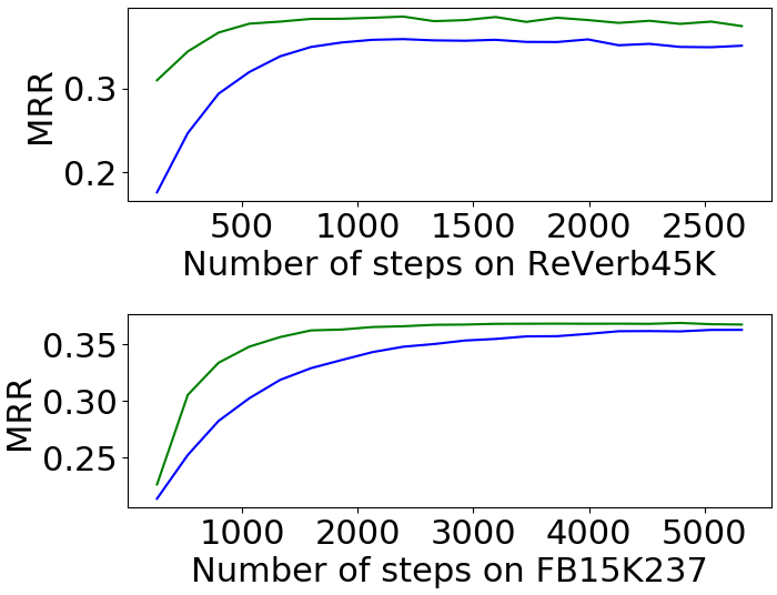
Figure 3: Comparing convergence of the overall best randomly initialized (blue) and pre-trained (green) models on ReVerb45K and FB15K237. Pre-trained models converge in fewer training steps despite a smaller learning rate.

		ReVerb20K			ReVerb45K
Model	Pre-trained?	MR	MRR	Hits@10	MR	MRR	Hits@10
NoEncoder_TuckER	no	$4862$	$.001$	$.002$	$8409$	$.001$	$.001$
	yes	$\mathit{1486}$	$\mathit{.012}$	$\mathit{.026}$	$\mathit{1737}$	$\mathit{.019}$	$\mathit{.041}$
NoEncoder_ConvE	no	$4600$	$.002$	$\mathit{.004}$	$8464$	$.001$	$\mathit{.001}$
	yes	$\mathit{1480}$	$\mathit{.003}$	$.000$	$\mathit{1962}$	$\mathit{.003}$	$\mathit{.001}$
NoEncoder_$5\star$E	no	$4795$	$.001$	$.000$	$8445$	$.001$	$.002$
	yes	$\mathit{1422}$	$\mathit{.005}$	$.000$	$\mathit{1701}$	$\mathit{.014}$	$\mathit{.011}$

Table 5: Comparison of the zero-shot performance of different models on the OKBC benchmarks ReVerb20K and ReVerb45K. The scores of each model are reported with and without pre-training on OlpBench, with the better of the two written in italics. Note that the model that was not pre-trained is equivalent to a random baseline.

Not only does pre-training allow us to train larger models, pre-trained models also require fewer training steps to obtain a similar performance, as seen in Figure 3. The experiments in the figure were done with the best hyperparameter setup for both pre-trained and randomly initialized model. Even though the pre-trained models were fine-tuned with a smaller learning rate, they converge in fewer steps, which can be attributed to the pre-training.

Finally, we highlight that language modelling as pre-training hardly justifies the enormous computational cost. On the majority of metrics, KG-Bert performs worse than models with fewer parameters and less pre-training, with a notable exception of a remarkable MR on the WN18RR dataset.

4.1 Zero-Shot Experiments

To understand better what kind of knowledge is transferred between the datasets, we investigate the zero-shot performance of pre-trained models on ReVerb20K and ReVerb45K, where the impact of pre-training was the strongest. If the improvement of pre-training was mainly due to the direct memorization of facts, the zero-shot performance should already be high without fine-tuning.

The results of the zero-shot evaluation are given in Table 5. We report the performance of all models with and without pre-training, the latter being equivalent to the random baseline. Note that since no fine-tuning takes place, the choice of the encoder for the evaluation does not matter. We thus chose to only evaluate one of them.

Observing the results, we see that pre-training the models results in a lower MR, but not necessarily a much higher MRR. Even when the increase of MRR happens, the difference is much smaller than when comparing fine-tuned models in Table 3. This implies that the improvement induced by pre-training likely does not happen only due to the memorization of facts from OlpBench. On the other hand, the MR of pre-trained models is comparable or even better than the MR of randomly initialized NoEncoder models, fine-tuned on the ReVerb datasets, reported in Table 3. Hence, pre-trained models carry a lot of “approximate knowledge”, which is consistent with earlier remarks on pre-training serving as a type of regularization.

Knowing that the ReVerb20K and ReVerb45K test sets consist of facts that contain at least one previously unseen entity or relation, this can be seen as out-of-distribution generalization. Comparing the zero-shot MRR results with the OlpBench results implies that while OKBC models are capable of out-of-domain generalization to unseen entities and relations, there is still space for improvement.

5 Related Work

In recent years, there have been several approaches to improve the performance of KBC algorithms through data augmentation, commonly through various levels of connection with unstructured text. Socher et al. (2013), for example, use pre-trained word embeddings to initialize their entity embeddings. Xie et al. (2016) make use of an encoder that generates an embedding given a description of the entity, and they show that their approach generalizes even to previously unseen entities. Yao et al. (2019) make use of a large-scale pre-trained transformer model to classify whether a fact is true. They rely on costly pre-training and do not generate embeddings for entities that could be used to incorporate background knowledge into natural language understanding systems Zhang et al. (2019).

Previous attempts at open knowledge base completion are tied to existing work on the canonicalization of knowledge bases. To canonicalize open knowledge bases, automatic canonicalization tools cluster entities using manually defined features Galárraga et al. (2014) or by finding additional information from external knowledge sources Vashishth et al. (2018). Gupta et al. (2019) use clusters obtained with these tools to augment entity embeddings for KBC. We note that Gupta et al. (2019) use RNN-based encoders to encode relations, but not to encode entities. Broscheit et al. (2020), on the other hand, introduce a model with RNN-based encoders for both entities and relations, similarly to our approach, however, they do not transfer beyond the introduced OlpBench dataset. Finally, Chandrahas and Talukdar (2021) use both KB canonicalization tools and large-scale pre-trained model Bert, combining their predictions to make a more informed decision.

The development of methods that improve predictions of KBC algorithms through data augmentation or transfer is tied to the advances in OIE and KBC methods. However, these are beyond the scope of this project; see the works by Niklaus et al. (2018) and Ruffinelli et al. (2020) for an overview.

6 Summary and Outlook

In this work, we have introduced a novel approach to transfer learning between various knowledge base completion datasets. The main strength of the introduced method is the ability to benefit from pre-training on uncanonicalized knowledge bases, constructed from facts, collected from unstructured text. Scaling the introduced method up would let us train large-scale pre-trained models that have already shown to be incredibly successful in natural language processing. We tested our method on $5$ different datasets, showing that pre-training improves the performance of models. Pre-training turned out to be particularly beneficial on small-scale datasets, where we were able to obtain the most significant gains, e.g., $6\%$ absolute increase of MRR and $65\%$ decrease of MR over the previously best method on ReVerb20K, despite not relying on large pre-trained models like Bert. There are several directions of future work, such as scaling of pre-training to larger models and datasets and investigating the impact of the encoder architecture.

Appendix A Metrics

This section contains a formal description of the metrics that were used to score the models. Let $\langle h,r,t\rangle$ be some test triple. Given $\langle h,r,?\rangle$, the model is used to rank all entities in the knowledge base from the most suitable to the least suitable tail, so that the entity no. $1$ is the most likely tail according to the model. All ranks are reported in the “filtered setting”, which means that all other known correct answers, other than $t$, are removed from this list to reduce noise. Let $r_{t}$ be the position or rank of the correct tail in this list. In ReVerb20K and ReVerb45K, there may be entities from the same cluster as $t$, equivalent to $t$. In this case, $r_{t}$ is the lowest of their ranks. The reciprocal rank of an example is then defined as $\frac{1}{r_{t}}$. The same process is repeated with the input $\langle?,r,t\rangle$ and the head entity.

The mean rank (MR) of the model is the average of all ranks across all test examples, both heads and tails. The mean reciprocal rank (MRR) is the average of all reciprocal ranks, both heads and tails. The Hits@N metric tells us how often the rank was smaller or equal to $N$. The related literature most commonly uses $1$, $3$, and $10$ for values of $N$, however, $5$, $30$, and $50$ are also occasionally reported.

Appendix B Detailed Experimental Setup

Following Ruffinelli et al. (2020), we use 1-N scoring for negative sampling and cross-entropy loss for all models. The Adam optimizer Kingma and Ba (2015) was used to train the network. We follow Dettmers et al. (2018) and Balažević et al. (2019) with the placement of batch norm and dropout in ConvE and TuckER, respectively, however, we simplify the setup by always setting all dropout rates to the same value to reduce the hyperparameter space. To find the best hyperparameters, grid search is used for all experiments to exhaustively compare all options. Despite numerous simplifications, we find that our re-implementations of the baselines (non-pre-trained NoEncoder models) perform comparable to the original reported values. The experiments were performed on a DGX-1 cluster, using one Nvidia V100 GPU per experiment.

Pre-training setup.

Pre-training was only done with GRU encoders, as discussed in Section 2.1. Due to the large number of entities in the pre-training set, 1-N sampling is only performed with negative examples from the same batch, and batches of size $4096$ were used, following Broscheit et al. (2020). The learning rate was selected from {$1\cdot 10^{-4},3\cdot 10^{-4}$}, while the dropout rate was selected from {$0.2,0.3$} for ConvE and {$0.3,0.4$} for TuckER. For 5^⋆E, the dropout rate was not used, but N3 regularization was Lacroix et al. (2018), its weight selected from {$0.1$,$0.03$}. For TuckER, models with embedding dimensions $100$, $200$, and $300$ were trained. We saved the best model of each dimension for fine-tuning. For ConvE, models with embedding dimensions $300$ and $500$ were trained, and the best model for each dimension was saved for fine-tuning. Following Gupta et al. (2019), we use a single 2d convolution layer with $32$ channels and $3\times 3$ kernel size. When the dimension of entities and relations is $300$, they were reshaped into $15\times 20$ inputs, while the $20\times 25$ input shapes were used for the $500$-dimensional embeddings. For 5^⋆E, models with embedding dimensions $200$ and $500$ were trained, and the best model for each dimension was saved for fine-tuning. Following Broscheit et al. (2020), we trained each model for $100$ epochs. Testing on the validation set is performed each $20$ epochs, and the model with the best overall mean reciprocal rank (MRR) is selected.

Fine-tuning setup.

Fine-tuning is performed in the same way as the pre-training, however, the models were trained for $500$ epochs, and a larger hyperparameter space was considered. More specifically, the learning rate was selected from {$3\cdot 10^{-5},1\cdot 10^{-4},3\cdot 10^{-4}$}. The dropout rate was selected from {$0.2,0.3$} for ConvE and {$0.3,0.4$} for TuckER. The weight of N3 regularization for the 5^⋆E models was selected from {$0.3,0.1,0.03$}. The batch size was selected from {$512,1024,2048,4096$}. The same embedding dimensions as for pre-training were considered.

Appendix C Full Results

This appendix contains detailed information on the best performance of all models. Table 6 contains the detailed information on the performance of the best models both on validation and test sets of the datasets. Table 7 includes information on the best hyperparameter setups and approximate training times. Note that the given times are approximate and are strongly affected by the selection of the hyperparameters as well as external factors.

		OlpBench validation								OlpBench test
Model	Pre-trained?	MR	MRR	H@1	H@3	H@5	H@10	H@30	H@50	MR	MRR	H@1	H@3	H@5	H@10	H@30	H@50
GRU_TuckER	no	$\mathbf{55.6K}$	$.058$	$.0.033$	$.060$	$.076$	$.104$	$.163$	$.195$	$\mathbf{57.2K}$	$.053$	$.029$	$.054$	$.070$	$.097$	$.155$	$.189$
GRU_ConvE	no	$57.6K$	$.047$	$.025$	$.048$	$.063$	$.090$	$.147$	$.179$	$\mathbf{57.2K}$	$.045$	$.022$	$.047$	$.060$	$.086$	$.140$	$.173$
GRU_$5\star$E	no	$60.1K$	$\mathbf{.060}$	$\mathbf{.034}$	$\mathbf{.061}$	$\mathbf{.078}$	$\mathbf{.109}$	$\mathbf{.171}$	$\mathbf{.205}$	$59.9K$	$\mathbf{.055}$	$\mathbf{.030}$	$\mathbf{.056}$	$\mathbf{.075}$	$\mathbf{.101}$	$\mathbf{.160}$	$\mathbf{.194}$
		ReVerb20K validation								ReVerb20K test
Model	Pre-trained?	MR	MRR	H@1	H@3	H@5	H@10	H@30	H@50	MR	MRR	H@1	H@3	H@5	H@10	H@30	H@50
NoEncoder_TuckER	no	$2532$	$.196$	$.160$	$.207$	$.230$	$.265$	$.318$	$.352$	$2611$	$.196$	$.157$	$.212$	$.236$	$.267$	$.332$	$.362$
	yes	$354$	$.367$	$.283$	$.400$	$.457$	$.529$	$.646$	$.702$	$303$	$.367$	$.295$	$.412$	$.466$	$.540$	$.659$	$.714$
NoEncoder_ConvE	no	$1376$	$.279$	$.233$	$.301$	$.329$	$.364$	$.423$	$.458$	$1419$	$.282$	$.227$	$.308$	$.338$	$.380$	$.442$	$.475$
	yes	$292$	$.392$	$.312$	$.423$	$.477$	$.546$	$.658$	$.706$	$227$	$.400$	$.313$	$.440$	$.491$	$.568$	$.680$	$.729$
NoEncoder_$5\star$E	no	$2213$	$.230$	$.180$	$.243$	$.279$	$.325$	$.421$	$.468$	$2301$	$.228$	$.174$	$.243$	$.278$	$.334$	$.429$	$.473$
	yes	$773$	$.249$	$.194$	$.263$	$.299$	$.353$	$.466$	$.528$	$780$	$.249$	$.191$	$.264$	$.302$	$.363$	$.471$	$.532$
GRU_TuckER	no	$646$	$.344$	$.277$	$.366$	$.409$	$.470$	$.564$	$.609$	$598$	$.357$	$.283$	$.391$	$.434$	$.493$	$.594$	$.639$
	yes	$283$	$.386$	$.305$	$.416$	$.465$	$.543$	$.660$	$.707$	$245$	$.397$	$.315$	$.429$	$.485$	$.558$	$.674$	$.720$
GRU_ConvE	no	$333$	$.377$	$.305$	$.405$	$.447$	$.516$	$.635$	$.683$	$334$	$.387$	$.305$	$.421$	$.471$	$.540$	$.648$	$.690$
	yes	$\mathbf{229}$	$.397$	$.317$	$.428$	$.477$	$.554$	$.671$	$.726$	$\mathbf{184}$	$.409$	$.326$	$.442$	$.499$	$.573$	$.687$	$.737$
GRU_$5\star$E	no	$430$	$.379$	$.302$	$.411$	$.454$	$.523$	$.639$	$.685$	$395$	$.390$	$.311$	$.422$	$.475$	$.546$	$.650$	$.697$
	yes	$243$	$\mathbf{.404}$	$\mathbf{.318}$	$\mathbf{.440}$	$\mathbf{.492}$	$\mathbf{.569}$	$\mathbf{.690}$	$\mathbf{.747}$	$202$	$\mathbf{.417}$	$\mathbf{.330}$	$\mathbf{.455}$	$\mathbf{.512}$	$\mathbf{.586}$	$\mathbf{.701}$	$\mathbf{.748}$
		ReVerb45K validation								ReVerb45K test
Model	Pre-trained?	MR	MRR	H@1	H@3	H@5	H@10	H@30	H@50	MR	MRR	H@1	H@3	H@5	H@10	H@30	H@50
NoEncoder_TuckER	no	$5097$	$.094$	$.077$	$.097$	$.109$	$.126$	$.160$	$.177$	$5135$	$.103$	$.088$	$.106$	$.116$	$.131$	$.164$	$.182$
	yes	$839$	$.305$	$.228$	$.335$	$.386$	$.453$	$.559$	$.610$	$780$	$.299$	$.220$	$.332$	$.386$	$.453$	$.557$	$.607$
NoEncoder_ConvE	no	$2741$	$.235$	$.180$	$.262$	$.293$	$.336$	$.406$	$.436$	$2690$	$.232$	$.179$	$.256$	$.288$	$.333$	$.400$	$.434$
	yes	$632$	$.353$	$.274$	$.384$	$.438$	$.506$	$.611$	$.662$	$666$	$.345$	$.267$	$.378$	$.432$	$.500$	$.601$	$.644$
NoEncoder_$5\star$E	no	$3653$	$.148$	$.116$	$.151$	$.174$	$.210$	$.289$	$.324$	$3460$	$.152$	$.123$	$.152$	$.174$	$.212$	$.289$	$.327$
	yes	$3233$	$.187$	$.151$	$.195$	$.222$	$.258$	$.320$	$.349$	$3279$	$.189$	$.153$	$.198$	$.224$	$.261$	$.325$	$.357$
GRU_TuckER	no	$1386$	$.304$	$.242$	$.330$	$.369$	$.423$	$.504$	$.545$	$1398$	$.302$	$.242$	$.323$	$.365$	$.420$	$.506$	$.546$
	yes	$761$	$.336$	$.263$	$.368$	$.413$	$.473$	$.570$	$.613$	$706$	$.331$	$.258$	$.359$	$.412$	$.477$	$.575$	$.618$
GRU_ConvE	no	$776$	$.351$	$.273$	$.387$	$.437$	$.501$	$.593$	$.631$	$824$	$.343$	$.268$	$.374$	$.424$	$.488$	$.584$	$.626$
	yes	$\mathbf{584}$	$.364$	$.285$	$.400$	$.452$	$.518$	$.620$	$.665$	$600$	$.357$	$.277$	$.393$	$.444$	$.509$	$.607$	$.651$
GRU_$5\star$E	no	$843$	$.362$	$.287$	$.394$	$.446$	$.511$	$.607$	$.649$	$836$	$.357$	$.278$	$.394$	$.443$	$.508$	$.605$	$.647$
	yes	$603$	$\mathbf{.385}$	$\mathbf{.305}$	$\mathbf{.421}$	$\mathbf{.474}$	$\mathbf{.542}$	$\mathbf{.642}$	$\mathbf{.683}$	$\mathbf{596}$	$\mathbf{.382}$	$\mathbf{.302}$	$\mathbf{.416}$	$\mathbf{.467}$	$\mathbf{.537}$	$\mathbf{.636}$	$\mathbf{.676}$
		FB15K237 validation								FB15K237 test
Model	Pre-trained?	MR	MRR	H@1	H@3	H@5	H@10	H@30	H@50	MR	MRR	H@1	H@3	H@5	H@10	H@30	H@50
NoEncoder_TuckER	no	$160$	$.366$	$.276$	$.399$	$.464$	$.547$	$.675$	$.727$	$166$	$.358$	$.265$	$.393$	$.458$	$.545$	$.669$	$.725$
	yes	$142$	$\mathbf{.369}$	$\mathbf{.277}$	$\mathbf{.403}$	$\mathbf{.468}$	$\mathbf{.555}$	$\mathbf{.680}$	$\mathbf{.732}$	$151$	$\mathbf{.363}$	$\mathbf{.269}$	$\mathbf{.398}$	$\mathbf{.464}$	$\mathbf{.550}$	$\mathbf{.678}$	$\mathbf{.733}$
NoEncoder_ConvE	no	$200$	$.326$	$.238$	$.356$	$.419$	$.508$	$.634$	$.690$	$212$	$.320$	$.230$	$.351$	$.417$	$.504$	$.634$	$.690$
	yes	$189$	$.332$	$.242$	$.363$	$.428$	$.513$	$.647$	$.703$	$200$	$.325$	$.233$	$.355$	$.421$	$.510$	$.645$	$.703$
NoEncoder_$5\star$E	no	$144$	$.358$	$.267$	$.393$	$.456$	$.542$	$.670$	$.723$	$152$	$.353$	$.260$	$.389$	$.454$	$.539$	$.666$	$.721$
	yes	$\mathbf{137}$	$.362$	$.270$	$.398$	$.462$	$.548$	$.672$	$.727$	$\mathbf{143}$	$.357$	$.264$	$.393$	$.459$	$.544$	$.670$	$.727$
GRU_TuckER	no	$\mathbf{137}$	$.355$	$.262$	$.391$	$.454$	$.539$	$.671$	$.724$	$144$	$.350$	$.256$	$.386$	$.451$	$.538$	$.666$	$.723$
	yes	$\mathbf{137}$	$.357$	$.264$	$.393$	$.454$	$.542$	$.670$	$.726$	$\mathbf{143}$	$.354$	$.260$	$.391$	$.453$	$.538$	$.668$	$.724$
GRU_ConvE	no	$161$	$.340$	$.249$	$.372$	$.433$	$.521$	$.653$	$.708$	$166$	$.334$	$.242$	$.368$	$.431$	$.519$	$.650$	$.705$
	yes	$151$	$.331$	$.241$	$.361$	$.423$	$.515$	$.652$	$.708$	$157$	$.327$	$.237$	$.359$	$.422$	$.513$	$.646$	$.704$
GRU_$5\star$E	no	$145$	$.351$	$.256$	$.387$	$.453$	$.540$	$.669$	$.725$	$150$	$.345$	$.249$	$.380$	$.449$	$.536$	$.667$	$.725$
	yes	$143$	$.351$	$.257$	$.386$	$.451$	$.537$	$.667$	$.722$	$145$	$.348$	$.254$	$.384$	$.450$	$.536$	$.666$	$.720$
		WN18RR validation								WN18RR test
Model	Pre-trained?	MR	MRR	H@1	H@3	H@5	H@10	H@30	H@50	MR	MRR	H@1	H@3	H@5	H@10	H@30	H@50
NoEncoder_TuckER	no	$3701$	$.469$	$.437$	$.483$	$.499$	$.524$	$.571$	$.595$	$4097$	$.468$	$.435$	$.483$	$.502$	$.528$	$.576$	$.595$
	yes	$3332$	$.470$	$.439$	$.479$	$.500$	$.529$	$.583$	$.604$	$3456$	$.467$	$.434$	$.480$	$.500$	$.529$	$.583$	$.604$
NoEncoder_ConvE	no	$6337$	$.429$	$.403$	$.437$	$.455$	$.479$	$.512$	$.530$	$6455$	$.429$	$.404$	$.440$	$.455$	$.479$	$.512$	$.530$
	yes	$5678$	$.433$	$.407$	$.442$	$.460$	$.483$	$.523$	$.542$	$5793$	$.435$	$.408$	$.444$	$.461$	$.486$	$.527$	$.545$
NoEncoder_$5\star$E	no	$2527$	$\mathbf{.492}$	$\mathbf{.450}$	$\mathbf{.505}$	$\mathbf{.531}$	$.574$	$.649$	$\mathbf{.680}$	$\mathbf{2450}$	$\mathbf{.492}$	$.448$	$\mathbf{.507}$	$\mathbf{.534}$	$\mathbf{.583}$	$\mathbf{.652}$	$.680$
	yes	$2576$	$\mathbf{.492}$	$\mathbf{.450}$	$.501$	$.528$	$\mathbf{.575}$	$\mathbf{.651}$	$\mathbf{.680}$	$2636$	$\mathbf{.492}$	$\mathbf{.450}$	$.504$	$.533$	$.582$	$\mathbf{.652}$	$\mathbf{.683}$
GRU_TuckER	no	$3201$	$.456$	$.428$	$.464$	$.484$	$.506$	$.553$	$.574$	$3262$	$.456$	$.429$	$.465$	$.483$	$.505$	$.551$	$.573$
	yes	$2637$	$.457$	$.422$	$.469$	$.490$	$.523$	$.579$	$.609$	$2790$	$.455$	$.418$	$.469$	$.494$	$.524$	$.577$	$.600$
GRU_ConvE	no	$4376$	$.431$	$.407$	$.439$	$.456$	$.477$	$.518$	$.538$	$4474$	$.428$	$.402$	$.438$	$.455$	$.474$	$.512$	$.533$
	yes	$5983$	$.400$	$.376$	$.410$	$.422$	$.444$	$.475$	$.493$	$6128$	$.399$	$.375$	$.409$	$.423$	$.441$	$.473$	$.491$
GRU_$5\star$E	no	$\mathbf{2444}$	$.456$	$.418$	$.463$	$.492$	$.533$	$.598$	$.629$	$2545$	$.452$	$.413$	$.462$	$.489$	$.527$	$.595$	$.629$
	yes	$2971$	$.426$	$.388$	$.440$	$.464$	$.494$	$.548$	$.575$	$3068$	$.420$	$.379$	$.437$	$.459$	$.488$	$.547$	$.573$

Table 6: Full results on both validation and test set of all datasets. In addition to the metrics reported in the paper, we also report H@N for $N\in\{1,3,5,10,30,50\}$, which appeared in related work. The best value in each column is written in bold.

		OlpBench
Model	Pre-trained?	dimension	learning rate	batch	dropout	N3 weight	time
GRU_TuckER	no	$300$	$1\cdot 10^{-4}$	$4096$	$0.3$	–	$5$ days
GRU_ConvE	no	$500$	$1\cdot 10^{-4}$	$4096$	$0.2$	–	$5$ days
GRU_$5\star$E	no	$500$	$1\cdot 10^{-4}$	$4096$	–	$0.03$	$12$ days
		ReVerb20K
Model	Pre-trained?	dimension	learning rate	batch	dropout	N3 weight	time
NoEncoder_TuckER	no	$300$	$3\cdot 10^{-5}$	$512$	$0.4$	–	$30$ min
	yes	$300$	$3\cdot 10^{-4}$	$512$	$0.3$	–	$30$ min
NoEncoder_ConvE	no	$300$	$3\cdot 10^{-4}$	$1024$	$0.3$	–	$30$ min
	yes	$500$	$1\cdot 10^{-4}$	$512$	$0.2$	–	$30$ min
NoEncoder_$5\star$E	no	$200$	$1\cdot 10^{-3}$	$512$	–	$0.3$	$30$ min
	yes	$500$	$3\cdot 10^{-4}$	$512$	–	$0.03$	$30$ min
Gru_TuckER	no	$300$	$3\cdot 10^{-3}$	$1024$	$0.4$	–	$30$ min
	yes	$300$	$3\cdot 10^{-5}$	$2048$	$0.4$	–	$30$ min
Gru_ConvE	no	$300$	$3\cdot 10^{-5}$	$512$	$0.3$	–	$30$ min
	yes	$500$	$3\cdot 10^{-5}$	$512$	$0.3$	–	$30$ min
Gru_$5\star$E	no	$200$	$3\cdot 10^{-4}$	$2048$	–	$0.1$	$30$ min
	yes	$500$	$1\cdot 10^{-4}$	$1024$	–	$0.1$	$30$ min
		ReVerb45K
Model	Pre-trained?	dimension	learning rate	batch	dropout	N3 weight	time
NoEncoder_TuckER	no	$100$	$1\cdot 10^{-3}$	$512$	$0.4$	–	$2.5$h
	yes	$300$	$3\cdot 10^{-4}$	$4096$	$0.3$	–	$2.5$h
NoEncoder_ConvE	no	$300$	$3\cdot 10^{-4}$	$512$	$0.3$	–	$2$h
	yes	$500$	$1\cdot 10^{-4}$	$2048$	$0.3$	–	$2.5$h
NoEncoder_$5\star$E	no	$200$	$1\cdot 10^{-3}$	$2048$	–	$0.3$	$3$h
	yes	$200$	$1\cdot 10^{-4}$	$512$	–	$0.1$	$3$h
Gru_TuckER	no	$300$	$1\cdot 10^{-3}$	$512$	$0.4$	–	$3$h
	yes	$300$	$3\cdot 10^{-4}$	$2048$	$0.4$	–	$3$h
Gru_ConvE	no	$300$	$1\cdot 10^{-4}$	$4096$	$0.3$	–	$2$h
	yes	$500$	$3\cdot 10^{-4}$	$2048$	$0.3$	–	$2.5$h
Gru_$5\star$E	no	$500$	$3\cdot 10^{-4}$	$1024$	–	$0.03$	$3$h
	yes	$500$	$3\cdot 10^{-4}$	$2048$	–	$0.1$	$3$h
		FB15K237
Model	Pre-trained?	dimension	learning rate	batch	dropout	N3 weight	time
NoEncoder_TuckER	no	$200$	$3\cdot 10^{-4}$	$1024$	$0.4$	–	$9.5$h
	yes	$300$	$3\cdot 10^{-5}$	$2048$	$0.4$	–	$9.5$h
NoEncoder_ConvE	no	$300$	$3\cdot 10^{-4}$	$2048$	$0.3$	–	$8.5$h
	yes	$500$	$3\cdot 10^{-4}$	$512$	$0.3$	–	$9$h
NoEncoder_$5\star$E	no	$500$	$1\cdot 10^{-4}$	$512$	–	$0.3$	$12$h
	yes	$500$	$1\cdot 10^{-4}$	$512$	–	$0.3$	$12$h
Gru_TuckER	no	$100$	$3\cdot 10^{-4}$	$512$	$0.4$	–	$13$h
	yes	$200$	$1\cdot 10^{-4}$	$1024$	$0.4$	–	$13$h
Gru_ConvE	no	$300$	$3\cdot 10^{-4}$	$512$	$0.3$	–	$11$h
	yes	$500$	$3\cdot 10^{-4}$	$512$	$0.3$	–	$12$h
Gru_$5\star$E	no	$500$	$1\cdot 10^{-4}$	$1024$	–	$0.1$	$24$h
	yes	$500$	$3\cdot 10^{-4}$	$512$	–	$0.1$	$24$h
		WN18RR
Model	Pre-trained?	dimension	learning rate	batch	dropout	N3 weight	time
NoEncoder_TuckER	no	$100$	$1\cdot 10^{-3}$	$512$	$0.3$	–	$7.5$h
	yes	$100$	$1\cdot 10^{-3}$	$512$	$0.3$	–	$7.5$h
NoEncoder_ConvE	no	$300$	$1\cdot 10^{-3}$	$512$	$0.3$	–	$8$h
	yes	$300$	$1\cdot 10^{-3}$	$512$	$0.3$	–	$8$h
NoEncoder_$5\star$E	no	$200$	$1\cdot 10^{-3}$	$512$	–	$0.3$	$8$h
	yes	$500$	$1\cdot 10^{-3}$	$1024$	–	$0.3$	$8$h
Gru_TuckER	no	$100$	$1\cdot 10^{-3}$	$512$	$0.3$	–	$6$h
	yes	$100$	$1\cdot 10^{-3}$	$1024$	$0.4$	–	$6$h
Gru_ConvE	no	$300$	$1\cdot 10^{-3}$	$1024$	$0.3$	–	$8.5$h
	yes	$500$	$1\cdot 10^{-3}$	$2048$	$0.3$	–	$8.5$h
Gru_$5\star$E	no	$500$	$3\cdot 10^{-4}$	$512$	–	$0.1$	$8.5$h
	yes	$500$	$1\cdot 10^{-3}$	$1024$	–	$0.3$	$8.5$h

Table 7: Best hyperparameter setups and training time of best models for all datasets.

References

- Abboud et al. (2020) Ralph Abboud, İsmail İlkan Ceylan, Thomas Lukasiewicz, and Tommaso Salvatori. 2020. BoxE: A box embedding model for knowledge base completion. In Proceedings of NeurIPS 34.
- Balažević et al. (2019) Ivana Balažević, Carl Allen, and Timothy M. Hospedales. 2019. TuckER: Tensor factorization for knowledge graph completion. In Proceedings of the 2019 EMNLP.
- Bordes et al. (2013) Antoine Bordes, Nicolas Usunier, Alberto Garcia-Duran, Jason Weston, and Oksana Yakhnenko. 2013. Translating embeddings for modeling multi-relational data. In Proceedings of NIPS 26.
- Broscheit et al. (2020) Samuel Broscheit, Kiril Gashteovski, Yanjie Wang, and Rainer Gemulla. 2020. Can we predict new facts with open knowledge graph embeddings? A benchmark for open link prediction. In Proceedings of the 58th ACL.
- Bruna et al. (2014) Joan Bruna, Wojciech Zaremba, Arthur Szlam, and Yann Lecun. 2014. Spectral networks and locally connected networks on graphs. In Proceedings of the 3rd ICLR.