Effects of anisotropy on strongly magnetized neutron and strange quark stars in general relativity

Abstract

We investigate the properties of anisotropic, spherically symmetric compact stars, especially neutron stars and strange quark stars, made of strongly magnetized matter. The neutron stars are described by SLy equation of state, the strange quark stars by an equation of state based on the MIT Bag model. The stellar models are based on an a priori assumed density dependence of the magnetic field and thus anisotropy. Our study shows that not only the presence of a strong magnetic field and anisotropy, but also the orientation of the magnetic field itself, have an important influence on the physical properties of stars. Two possible magnetic field orientations are considered, a radial orientation, where the local magnetic fields point in the radial direction, and a transverse orientation, where the local magnetic fields are perpendicular to the radial direction. Interestingly, we find that for a transverse orientation of the magnetic field, the stars become more massive with increasing anisotropy and magnetic field strength and increase in size, since the repulsive, effective anisotropic force increases in this case. In the case of a radially orientated magnetic field, however, the masses and radii of the stars decrease with increasing magnetic field strength, because of the decreasing effective anisotropic force. Importantly, we also show that in order to achieve hydrostatic equilibrium configurations of magnetized matter, it is essential to account for both the local anisotropy effects as well as the anisotropy effects caused by a strong magnetic field. Otherwise, hydrostatic equilibrium is not achieved for magnetized stellar models.

1 Introduction

Compact stars present unique astrophysical laboratories to study the nature of matter (and several astrophysical phenomena) under extreme physical conditions (Glendenning, 1996; Weber, 2017). Neutron stars (NSs) and Strange Quark stars (SQSs) represent the ultra-dense classes of compact stars. Magnetic flux conservation during stellar collapse leads to the presence of ultra-strong magnetic fields inside of compact stars. Some researchers have found that at the center of inhomogeneous, ultradense and gravitationally bound compact stars, the magnetic field may be as high as $\sim 10^{19}$ G (Yuan & Zhang, 1998; Tatsumi, 2000; Ferrer et al., 2010). However, from the available observational evidence, it is difficult to confirm the strength of the magnetic field inside of compact stars, which urges researchers to develop suitable theoretical models that help to investigate appropriately the effects of high magnetic fields on the physical parameters of compact stellar objects. Evidently, to study the effects that high magnetic fields have on compact stars, it is essential to carry out such a study in the realm of general relativity (GR). Following the pioneering works of Tolman (1939); Oppenheimer & Volkoff (1939) (TOV), many researchers have investigated the properties of NSs and SQSs based on the GR hydrostatic equilibrium equation derived by TOV (Bowers & Liang, 1974; Hillebrandt & Steinmetz, 1976; Mak & Harko, 2002; Weber, 2005; Negreiros et al., 2009; Weber et al., 2014; Arbañil & Malheiro, 2016; Deb et al., 2017, 2018).

Since the ground breaking observation of radio pulsars by Hewish et al. (1968), NSs remain to be one of the most studied astrophysical objects, which are assumed to be the possible sources of high-energy emission. The typical values of the surface magnetic field as inferred from simple magnetic dipole models and spin-down rates are in the range $10^{8}-10^{13}$ G (Taylor et al., 1993; Alpar et al., 1982). Note that among the radio pulsars, PSR J1847$-$0130 exhibits a strong magnetic field of $B=9.4\times{14}^{13}$ G (McLaughlin et al., 2003). On the other hand, besides the X-ray luminosities observed from the anomalous X-ray pulsars (AXPs), the inferred periods of AXPs and soft-$\gamma$ repeaters (SGRs) suggest that such NSs have even larger surface magnetic fields of $10^{14}-10^{15}$ G (Paczynski, 1992; Duncan & Thompson, 1992; Thompson & Duncan, 1996; Melatos, 1999). Neutron stars with such high surface magnetic fields are popularly known as magnetars. Further on, several interesting studies (Usov, 1992; Kluźniak & Ruderman, 1998; Wheeler et al., 2000; Starling et al., 2009; Cenko et al., 2010) have predicted that magnetars are the probable source of $\gamma$-ray bursts and they require higher magnetic field such as $10^{16}-10^{17}$ G to initiate the Poynting flux-dominated jets. Although till now only around 30 magnetars have been detected, it is speculated that these astrophysical objects may account for $10\%$ of the NSs population (Kouveliotou et al., 1998). For NSs, the effects of a strong magnetic field on the ultra-dense electron gases in their interiors have been studied in several papers  (Canuto & Ventura, 1977; Fushiki et al., 1989; Abrahams & Shapiro, 1991; Fushiki et al., 1992; Roegnvaldsson et al., 1993). Studies of dense and strongly magnetized nuclear matter have also been carried out by Chakrabarty et al. (1997); Bandyopadhyay et al. (1998); Broderick et al. (2000); Suh & Mathews (2001); Harding & Lai (2006); Chen et al. (2007); Rabhi et al. (2008) and references therein. Finally we mention that studies of NSs with different magnetic field configurations, viz., toroidal, poloidal, or mixed were carried out by Bocquet et al. (1995); Cardall et al. (2001); Pili et al. (2014).

Because of its profound significance for strong interaction physics and astrophysics, the possible existence of SQS has attracted great scientific interest over the past three decades. SQSs are hypothetical compact stellar objects made completely of strange quark matter (SQM). Such matter consists entirely of deconfined up ($u$), down ($d$) and strange ($s$) quarks, which, according to the SQM hypothesis, could be lower in energy than nuclear matter and thus be the true ground state of the strong interaction (Bodmer, 1971; Witten, 1984; Terazawa, 1990). Various researchers have studied the properties of SQSs (see, for instance,  Itoh 1970; Alcock et al. 1986; Haensel et al. 1986; Alcock & Olinto 1988; Madsen 1999; Bombaci et al. 2004; Weber 2005; Staff et al. 2007; Herzog & Röpke 2011). Furthermore, theoretical studies have shown that the birth of SQSs could occur through the conversion of NSs to SQSs within a few milliseconds via a strong deflagration process, which leads to the emission of a powerful neutrino signal (Martem’yanov, 1994; Bombaci et al., 2004; Staff et al., 2007; Herzog & Röpke, 2011). A distinguishing feature between NSs and SQSs is that the radii of the latter become monotonically smaller with decreasing star mass, which is not the case for NSs (Alcock et al., 1986; Alcock & Olinto, 1988; Kapoor & Shukre, 2001). In the past, it has been speculated that compact stars such as 4U 1728-34, 4U 1820-30, SAX J1808.4C3658, Her X-1 and RX J1856.5C3754 could be SQS candidates (Weber, 2005). Hence, it will be interesting to investigate the GR effects on strongly magnetized SQSs. Important studies which have examined the effects of strong magnetic fields on SQSs have been carried out by Chakrabarty (1996); Chaichian et al. (2000); González Felipe et al. (2008); Menezes et al. (2009a, b); Rabhi et al. (2009).

Ruderman (1972) has shown that when the nuclear matter in the stellar interior reaches a density beyond ${10}^{15}~{}{\rm g/cm}^{3}$, interactions become relativistic, and the presence of a type-P superfluid leads to a pressure anisotropy in the stars. However, Bowers & Liang (1974) in their study strongly argued against the over-simplistic assumption that compact stars are composed of only an isotropic perfect fluid. They presented the non-negligible effects of a local anisotropy on the physical parameters of compact stars, such as maximum equilibrium mass and surface redshift, by generalizing the TOV equations in terms of a local anisotropy. Letelier (1980) and Bayin (1982) strongly argued that the presence of two (or more) fluids or a mixture thereof in compact stars, may be the possible reason for pressure anisotropy, which Herrera & Santos (1997) confirmed later. Further, anisotropy may be caused by phase transitions (Sokolov, 1980; Carter & Langlois, 1998) in the interiors of compact stars, when the matter forms superfluid or superconducting states. Some works (Barreto & Rojas, 1992; Barreto, 1993) also showed that the presence of viscosity might be the possible source of local anisotropy within dense compact stars. Other investigations revealed additional reasons for the existence of local anisotropy, such as pion condensation (Sawyer, 1972; Dev & Gleiser, 2000), the existence of a solid core at densities $10^{14-15}~{}{\rm g/cm}^{3}$ (Cameron & Canuto, 1974; Canuto, 1974, 1977), and the presence of a type-3A superfluid (Kippenhahn & Weigert, 1990), which are considered to offer a more realistic view of the structure of the ultra-dense cores of compact stellar objects. For a further detailed understanding of the mechanisms that produce anisotropies, one may see the seminal articles (Herrera & Santos, 1997; Dev & Gleiser, 2000) and references therein. Further, to emphasize the relevance of local anisotropy, several recent articles (Corchero, 2001; Ivanov, 2002; Mak & Harko, 2003; Schunck & Mielke, 2003; Usov, 2004; Chaisi & Maharaj, 2005; Varela et al., 2010; Rahaman et al., 2010, 2011, 2012; Silva et al., 2015; Arbañil & Malheiro, 2016; Deb et al., 2017, 2018) may also be recalled, where the effects of local anisotropy on spherically symmetric compact stars were studied in detail. Ferrer et al. (2010) showed that the presence of a strong magnetic field may also lead to anisotropy in compact stars by breaking the spatial rotational $[{\mathcal{O}}(3)]$ symmetry, which later Isayev & Yang (2011, 2012) confirmed in their articles.

Interestingly, researchers (Bandyopadhyay et al., 1997, 1998; Broderick et al., 2000; Cardall et al., 2001; Menezes et al., 2009a, b; Ryu et al., 2010; Paulucci et al., 2011; Ryu et al., 2012; Dexheimer et al., 2014; Casali et al., 2014; Hou et al., 2015; Kayanikhoo et al., 2020) still do not agree unanimously on whether the maximum mass of a compact stellar object increases or decreases due to the presence of a strong magnetic field and it remains still an important open issue that needs to be resolved. Chu et al. (2014) tried to address this issue by introducing the idea of magnetic field orientation. When the local magnetic fields are directed towards the radial direction, they are termed radially oriented (RO), and when the magnetic fields are randomly oriented in the direction perpendicular to the radial direction (say along $\theta$ direction), they are referred to as transversely orientated (TO). Chu et al. (2014) showed in their study that not only the strength of the magnetic field but also its orientation has a significant effect on the maximum mass of a compact stellar object. However, it is important to point out that in their study, neither the effect of the magnetic field nor of the magnetic field orientation on the TOV equation has been taken into account. Hence, no effect of the orientation of the magnetic field was observed, with the exception of a change in the total stellar mass. This is not expected in reality. Hence, it will be interesting to investigate the properties of anisotropic compact stars by considering the effects of magnetic field orientations and its spatial distribution in the TOV equation. Therefore, in the present study, we consider the presence of the effective anisotropy that is arising due to (i) the local anisotropy of the fluid, and (ii) the presence of a strong magnetic field. Note that the magnetic field strength at the surface of magnetars is relatively weak, and it gradually increases up to several orders to reach its maximum value at the center (see Melatos 1999; Makishima et al. 2014; Dexheimer et al. 2017). Although the pressure anisotropy inside the magnetars may not be very large, the present study shows that the consideration of anisotropy offers a more generalized TOV equation to calculate the properties of magnetized anisotropic compact stars and also the effective anisotropy due to both the fields and matter plays a crucial role to ensure stability at the stellar center.

The present article is arranged as follows. In the next section, we discuss the basic formalism and the modified hydrostatic equilibrium equations of highly magnetized compact stellar objects. To close the system of equations, we consider an ansatz for the anisotropy which is introduced in subsection 2.1. The equation of state (EOS) is discussed in subsection 2.2 and the functional form of the density-dependent magnetic field is considered in subsection 2.3. In Section 3 we discuss the achieved results. Further, possible future directions of our study are presented in Section 4. We conclude this work with a brief discussion in Section 5.

2 Basic Formalism and Structure equations for magnetized compact stars

To describe the interior spacetime of static, spherically symmetric compact stellar objects, we consider the metric

$$\mathrm{d}s^{2}=e^{\nu(r)}\mathrm{d}t^{2}-e^{\lambda(r)}\mathrm{d}r^{2}-r^{2}(\mathrm{d}\theta^{2}+\sin^{2}\theta\mathrm{d}\phi^{2}),$$ (1)

where $\nu(r)$ and $\lambda(r)$ are the metric potentials.

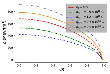
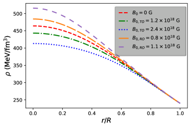
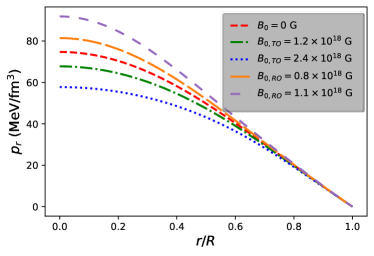
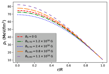
Figure 1: Variation of (i) matter density ($\rho$), (ii) radial pressure $(p_{r})$, and (iii) tangential pressure $(p_{t})$ with radial coordinate $r/R$ for $2.01\pm 0.04~{}M_{\odot}$ (Antoniadis et al., 2013) NS candidate PSR J0348+0432 (panels on the left) and $1.97\pm 0.04~{}M_{\odot}$ (Demorest et al., 2010) SQS candidate PSR J1614$-$2230 (panels on the right). Here and in what follows $\kappa=0.5$, $\eta=0.2$, $\gamma=2$ and $\mathcal{B}=60~{}\mathrm{MeV/{fm^{3}}}$.

The energy-momentum tensor of the system is given by

$$T^{\mu\nu}=T^{\mu\nu}_{m}+T^{\mu\nu}_{f},$$ (2)

where $T^{\mu\nu}_{m}$ and $T^{\mu\nu}_{f}$ represent the contributions due to the matter and field, respectively, which are given by

$$T^{\mu\nu}_{m}=(\rho+{p_{t}})u^{\mu}u^{\nu}-{p_{t}}g^{\mu\nu}+\left({p_{r}}-{p_{t}}\right)v^{\mu}v^{\nu}$$

$$\hskip 99.58464pt+\frac{1}{2}\left(\mathcal{M}^{\mu\alpha}F^{\nu}_{\alpha}+\mathcal{M}^{\nu\alpha}F^{\mu}_{\alpha}\right),$$ (3)

$$T^{\mu\nu}_{f}=-\frac{1}{4\pi}F^{\mu\alpha}F^{\nu}_{\alpha}+\frac{1}{16\pi}g^{\mu\nu}F^{\beta\sigma}F_{\beta\sigma},$$ (4)

where $u^{\mu}=\delta^{\mu}_{0}e^{-\nu(r)/2}$ which is the time-like unit vector denoting the fluid 4-velocity of matter, whereas $v^{\mu}=\delta^{\mu}_{1}e^{-\lambda(r)/2}$ represents the space-like unit vector in the radial direction. They satisfy $u^{\mu}u_{\mu}=-v^{\mu}v_{\mu}=1$ and $u^{\mu}v_{\mu}=0$. The quantities $\rho$, $p_{r}$ and $p_{t}$ represent the energy density of matter, the radial pressure in the direction of $v^{\mu}$ and the tangential pressure orthogonal to $v_{\mu}$, respectively. The quantities $\mathcal{M}^{\mu\nu}$ and $F^{\mu\nu}$ represent the magnetization tensor and the Maxwell tensor, respectively, and $g_{\mu\nu}$ is the metric tensor. Now considering that in the bulk matter there are no macroscopic charges, we can neglect the effects due to the electric field and immediately obtain from the Eqs. (2) and (4)

$$T^{\mu\nu}_{m}=(\rho+{p_{t}})u^{\mu}u^{\nu}-{p_{t}}g^{\mu\nu}+\left({p_{r}}-{p_{t}}\right)v^{\mu}v^{\nu}$$

$$\hskip 85.35826pt+\mathcal{M}B\left(g^{\mu\nu}-u^{\mu}u^{\nu}+\frac{B^{\mu}B^{\nu}}{B^{2}}\right),$$ (5)

$$T^{\mu\nu}_{f}=\frac{B^{2}}{4\pi}\left(u^{\mu}u^{\nu}-\frac{1}{2}g^{\mu\nu}\right)-\frac{B^{\mu}B^{\nu}}{4\pi},$$ (6)

where $\mathcal{M}$ is the magnetization per unit volume and $B^{\mu}B_{\mu}=-B^{2}$. Ferrer et al. (2010) and Sinha et al. (2013) found in their works that the magnetization is at least one order of magnitude smaller than the magnetic pressure and that magnetization has no effect on the physical properties of magnetized matter. Hence the magnetization effect is very small and will therefore be neglected in the numerical results of our study. Importantly, we assume the field strengths to be such that they do not or only minimally effect the spherical shape of a compact star. Moreover, toroidally dominated magnetized compact stars do not deviate much from spherical symmetry (Das & Mukhopadhyay, 2015b; Subramanian & Mukhopadhyay, 2015; Kalita & Mukhopadhyay, 2019). We therefore make use of the standard form of the TOV equation for the description of magnetized compact stars in the present work.

The system density $(\widetilde{\rho})$, which is the sum of the contribution from the matter and field, is given by

$$\widetilde{\rho}=\rho+\frac{B^{2}}{8\pi}.$$ (7)

Depending on the magnetic field orientation, the system’s parallel pressure along the magnetic field reads

$$p_{\parallel}=\begin{cases}p_{r}-\frac{B^{2}}{8\pi},\hskip 28.45274pt&\textrm{for~{} RO}\\ p_{t}-\frac{B^{2}}{8\pi}.\hskip 28.45274pt&\textrm{for~{} TO}\end{cases}$$ (8)

Similarly, the system transverse pressure perpendicular to the magnetic field is given by

$$p_{\bot}=\begin{cases}p_{t}+\frac{B^{2}}{8\pi},\hskip 28.45274pt&\textrm{for~{} RO}\\ p_{r}+\frac{B^{2}}{8\pi}.\hskip 28.45274pt&\textrm{for~{} TO}\end{cases}$$ (9)

Note that $p_{t}$ stands for the pressure either in the polar or in the azimuthal directions in spherical symmetry.

The mass function of a star in the presence of a magnetic filed is defined as

$$m\left(r\right)=\int_{0}^{r}4\pi r^{2}\widetilde{\rho}\;\mathrm{d}r.$$ (10)

Finally, the conservation of the energy momentum tensor is expressed as

$$\nabla_{\mu}T^{\mu\nu}=0.$$ (11)

Following Eqs. (1), (2), (2)-(11), the essential stellar structure equations needed to describe static, anisotropic, spherically symmetric compact objects in the presence of a strong magnetic field take the form

$$\frac{\mathrm{d}m}{\mathrm{d}r}=4\pi\left(\rho+\frac{B^{2}}{8\pi}\right)r^{2},$$ (12)

$$\begin{cases}{\frac{{\rm d}p_{r}}{{\rm d}r}}=\frac{-\left(\rho+p_{{r}}\right)\frac{4\pi{r}^{3}\left(p_{{r}}-{\frac{{B}^{2}}{8\pi}}\right)+m}{r\left(r-2m\right)}+\frac{2}{r}\Delta}{\left[1-\frac{\rm d}{{\rm d}\rho}\left(\frac{B^{2}}{8\pi}\right)\frac{{\rm d}\rho}{{\rm d}{p_{r}}}\right]},\hskip 26.74565pt\textrm{for RO}\\ {\frac{{\rm d}p_{r}}{{\rm d}r}}=\frac{-\left(\rho+p_{{r}}+\frac{B^{2}}{4\pi}\right)\frac{4\pi{r}^{3}\left(p_{{r}}+{\frac{{B}^{2}}{8\pi}}\right)+m}{r\left(r-2m\right)}+\frac{2}{r}\Delta}{\left[1+\frac{\rm d}{{\rm d}\rho}\left(\frac{B^{2}}{8\pi}\right)\frac{{\rm d}\rho}{{\rm d}{p_{r}}}\right]},\hskip 5.69046pt\textrm{for TO}\end{cases}$$ (13)

where $\Delta=\left(p_{t}-p_{r}+\frac{B^{2}}{4\pi}\right)$ or $\left(p_{t}-p_{r}-\frac{B^{2}}{8\pi}\right)$, which denote the effective anisotropy of stellar structures for RO or TO, respectively.

For the non-magnetized case, i.e., $B=0$, Eq. (13) reduces to the standard form of the TOV equation (Bowers & Liang, 1974; Herrera & Barreto, 2013). It is important to mention that throughout the present investigation, we consider field magnitudes $<3\times{10^{18}}$ G, hence the effects of Landau quantization are negligible. In fact, the effects due to Landau quantization become significant only for fields larger than ${10}^{19}$ G (Sinha et al., 2013). Therefore, following Sinha et al. (2013), we consider Landau quantization effects to be negligible. The anisotropic contribution due to the magnetic field, however, will still be there since the difference between the parallel and transverse pressures is proportional to the square of the field magnitude. Besides, one should not forget the local anisotropy of the fluid.

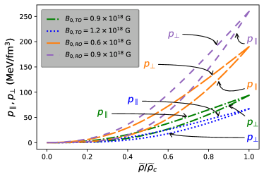
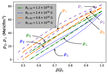
Figure 2: Variation of parallel pressure $(p_{\parallel})$ and transverse pressure $(p_{\bot})$ with the system density $(\widetilde{\rho})$, normalized to the central system density $(\widetilde{\rho}_{c})$, for $2.01\pm 0.04~{}M_{\odot}$ (Antoniadis et al., 2013) NS candidate PSR J0348+0432 and $1.97\pm 0.04~{}M_{\odot}$ (Demorest et al., 2010) SQS candidate PSR J1614$-$2230. The upper panel features NS pressure profiles, whereas the lower panel presents SQS pressure profiles. The dotted, dash-dotted, long-dashed and short-dashed curves correspond to $B_{0}=2.4\times{10}^{18}$ G (TO), $B_{0}=1.2\times{10}^{18}$ G (TO), $B_{0}=0.8\times{10}^{18}$ G (RO) and $B_{0}=1.1\times{10}^{18}$ G (RO), respectively.

2.1 Ansatz for Anisotropy

Further, we require a functional form for the anisotropy $(\Delta)$ to close the system of equation in such a way that we may include the anisotropic effect due to both the local anisotropy of the fluid and the presence of a strong magnetic field. Unfortunately, there is no available explicit form of anisotropy in the existing literature derived directly from the microscopic theory, which can explain the combined anisotropic effects due to both the fluid and magnetic field. To overcome this delicate issue, we consider a phenomenological approach based on the essential assumptions given bellow.

(i) At the stellar center the hydrodynamic force $F_{h}$ and gravitational force $F_{g}$ are zero. To maintain the stability of the system via equilibrium of the forces (non-diverging nature), the anisotropic force essentially should be zero at the center, which implies that the anisotropy must vanish quadratically at the center.

(ii) The anisotropy should vary with position inside the system and also depend non-linearly on $p_{r}$ (Bowers & Liang, 1974; Silva et al., 2015).

(iii) Based on the present study, the functional form of the anisotropy should include the anisotropic effects due to both the local anisotropy of the fluid and the presence of a strong magnetic field. It is also important to include the effects due to magnetic field orientation.

Bowers & Liang (1974) derived a general parametric form for $\Delta$ in general relativity for a spherically symmetric star, which is consistent with the above mentioned essential assumptions (i) to (iii). In the years following the Bowers and Liang paper, hundreds of articles have investigated the effects of anisotropy for compact stars using this parametric form of anisotropy, which has become widely accepted within the community. To include the effects of the magnetic field and its orientation, here we modify the Bowers-Liang anisotropic form, which reads

$$\Delta=\begin{cases}\kappa\frac{\left(\rho+p_{r}\right)\left(\rho+3\,p_{r}-\frac{B^{2}}{4\pi}\right)}{\left(1-\frac{2m}{r}\right)}r^{2},\hskip 42.67912pt\textrm{for RO}\\ \kappa\frac{\left(\rho+p_{r}+\frac{B^{2}}{4\pi}\right)\left(\rho+3\,p_{r}+\frac{B^{2}}{2\pi}\right)}{\left(1-\frac{2m}{r}\right)}r^{2},\hskip 22.76228pt\textrm{for TO}\end{cases}$$ (14)

where the dimensionless constant $\kappa$ controls the strength of the anisotropy in the system. Note that we consider the parametric values of $\kappa$ well within its limiting values given by $\left[-\frac{2}{3},\frac{2}{3}\right]$ (Silva et al., 2015). Note that Ferrer et al. (2010) introduced “anisotropy, which leads to the distinction between longitudinal- and transverse-to-the-field pressures”. To this end, our study has focused on the important fact that the anisotropy necessarily should be zero at the center in the case of magnetized compact stars and the stellar models with non-zero anisotropies at the center would have unstable cores [see Eq. (12)], which would eliminate such theoretical models.

The chosen parametric form for the anisotropy based on a phenomenological approach is consistent with the essential physical assumptions (i) to (iii) and has been widely accepted by the community. It includes the effects of magnetic fields and their orientations and constitutes currently the best possible physically viable way of solving the hydrostatic equilibrium equations of magnetized compact stars.

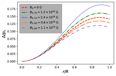
Figure 3: Anisotropy profiles $\Delta$, normalized to central pressure $(p_{c})$, for $2.01\pm 0.04~{}M_{\odot}$ (Antoniadis et al., 2013) NS candidate PSR J0348+0432 and $1.97\pm 0.04~{}M_{\odot}$ (Demorest et al., 2010) SQS candidate PSR J1614$-$2230. The top panel is for NSs, the bottom panel is for SQSs.

2.2 Equation of state

Next we consider the relation between $\rho$ and $p_{r}$, known as EOS, to close our system of equations. By providing the EOS of matter together with the functional form for the anisotropy of the system, the stellar structure equations (12) and (13) can be then solved numerically. In order to obtain solutions of the coupled stellar structure equations, it is required to integrate Eqs. (12) and (13) simultaneously, from the stellar center to the surface.

We consider SLy EOS, which is moderately stiff in classification. Based on Skyrme-type energy density functional, Douchin & Haensel (2001) proposed SLy EOS, which is widely used in the literature to discuss NSs. Note that SLy EOS is equally consistent in the NS core and the crust.

The phenomenological MIT bag model EOS was introduced by Chodos et al. (1974) to study strongly interacting particles, viz., hadrons. In our work, we use the MIT bag model EOS to describe (absolutely stable) SQM and to compute the properties of SQSs. The $u$, $d$, and $s$ quarks are treated as massless but relativistic particles confined inside a spherical bag, in which case the EOS of SQM is given by

$$p_{r}=\frac{1}{3}\left(\rho-4\,\mathcal{B}\right),$$ (15)

where $\mathcal{B}$ denotes the MIT bag constant. Our numerical results are computed for a bag constant value of $\mathcal{B}=60~{}\mathrm{MeV/{fm^{3}}}$ $(\mathcal{B}^{1/4}=146~{}\mathrm{MeV})$, which corresponds to SQM that is strongly bound (of strange quark mass $\sim 100$ MeV) with respect to ordinary nuclear matter and ${}^{56}{\text{F}e}$ (Farhi & Jaffe, 1984; Weber, 2005). As required by SQM hypothesis (Bodmer, 1971; Witten, 1984; Terazawa, 1990), the energy per baryon of 2-flavor ($u$, $d$) quark matter for this value of the bag constant is higher than the energy per baryon of nuclear matter and ${}^{56}{\text{F}e}$. We also note that this $\mathcal{B}$ value lies within the range of $57-94~{}\mathrm{MeV/{fm^{3}}}$, which is $(145\lesssim\mathcal{B}^{1/4}\lesssim 164~{}\mathrm{MeV})$ frequently studied in the literature dealing with absolutely stable strange quark matter (Farhi & Jaffe, 1984; Alcock et al., 1986; Burgio et al., 2002; Jaikumar et al., 2006; Bordbar et al., 2012; Maharaj et al., 2014; Arbañil & Malheiro, 2016; Moraes et al., 2016; Alaverdyan & Vartanyan, 2017; Lugones & Arbañil, 2017; Deb et al., 2019).

Figure 4: Variation of magnetic field $B$ with radial coordinate $r/R$, for $2.01\pm 0.04~{}M_{\odot}$ (Antoniadis et al., 2013) NS candidate PSR J0348+0432 and $1.97\pm 0.04~{}M_{\odot}$ (Demorest et al., 2010) SQS candidate PSR J1614$-$2230. The upper and lower panels represent NS and SQS magnetic field profiles, respectively.

2.3 Profile for density-dependent magnetic fields

To solve Eqs. (12) and (13) simultaneously, one needs to close the system of equations by specifying a parametric form of the magnetic field strength. To mimic the spatial dependence of the magnetic field strength, which varies from the stellar center to the surface, in the present study we consider a density-dependent parametric form for the magnetic field strength which was conceptualized by Bandyopadhyay et al. (1997, 1998) and later was widely applied in literature (Menezes et al., 2009a; Ryu et al., 2010, 2012; Sinha et al., 2013; Chu et al., 2014, 2015; Isayev, 2018; Roy et al., 2019; Aguirre, 2020; Baruah Thapa et al., 2020).

Therefore, following Bandyopadhyay et al. (1997, 1998), we choose the profile for the density-dependent magnetic field in such a way that the magnetic field at the stellar core, $B_{c}$, complies with the virial theorem and the surface magnetic field, $B_{s}$, fits observed values. This profile is given by

$$B(\rho)=B_{s}+B_{0}\left[1-\exp\left\{-\eta\left(\frac{\rho}{\rho_{0}}\right)^{\gamma}\right\}\right],$$ (16)

where $B_{0}$ is a parameter that has the same dimension as the magnetic field strength, and the dimensionless parameters $\eta$ and $\gamma$ control how the magnetic field decays from its maximum value at the center to the minimum value at the surface. More precisely, $\eta$ controls the field decay at the saturation density, and the width of the transition is controlled by $\gamma$. Here, $\rho_{0}$ denotes the normal nuclear matter density. However, one may note that although Eq. (16) is applicable to NSs, for SQSs, where the surface density is $\rho_{s}\neq 0$, a modification of the magnetic field profile is required to ensure that the asymptotic value for $B_{s}$ is obtained at the surface, given by

$$B(\rho)=B_{s}+B_{0}\left[1-\exp\left\{-\eta\left(\frac{\rho-\rho_{s}}{\rho_{0}}\right)^{\gamma}\right\}\right].$$ (17)

In the present study, we shall consider values of $B_{s}$ given by $10^{13}$ and $10^{15}$ G for NSs and SQSs, respectively. However, we found that our results are not sensitive to the particular choice of the value of $B_{s}$.

2.4 Consistency of Maxwell’s equation with the magnetic field orientations

Chu et al. (2014, 2015) in their works showed that magnetic field orientations have a significant effect on spherically symmetric compact stars. Following their work, we offer a more general model by considering the same magnetic field orientations, such as “radial orientation” when the local magnetic fields orient themselves along the radial direction and the “transverse orientation” when the local magnetic fields are oriented perpendicularly to the radial direction. Now we show in a straightforward way that there is no violation of $\overrightarrow{\nabla}\cdot\overrightarrow{B}=0$ for the present interest of magnetic field orientations:

(i) Radial orientation: For a radial orientation, the magnetic field takes the form

$$\overrightarrow{B}=\left(B_{r},0,0\right).$$ (18)

Now,

$$\overrightarrow{\nabla}\cdot\overrightarrow{B}=0\Rightarrow\frac{1}{r^{2}}\frac{\partial}{\partial r}\left(r^{2}B_{r}\right)=0\Rightarrow B_{r}=\frac{K}{r^{2}}.$$ (19)

Here $K$ cannot be a pure constant in order to avoid absurd possibility of magnetic monopole. Hence, $K$ could be $K\left(\theta,\phi\right)$. Hence, $B_{r}$ could be thought of as $B_{r}={K{\rm sign}(\cos\theta)}/r^{2}$, i.e., with upper hemisphere $+K$ and lower hemisphere $-K$. This physically implies that the field lines coming out of the upper hemisphere and entering through the lower hemisphere of the star, hence having split monopole type in nature. Of course, this is an approximate modeling of the magnetic field in a star assuming to be spherical in shape. However, for the present purpose, this will not pose any practical hindrance in order to understand the physics.

For the ease of understanding, let us choose Minkowski space, which leads the spatial components to

$$M^{ij}=\frac{B^{2}}{8\pi}\delta^{ij}-\frac{B^{i}B^{j}}{4\pi}.$$ (20)

From Eq. (20) one can see that $M^{rr}=\frac{B^{2}}{8\pi}-\frac{B^{2}}{4\pi}=-\frac{B^{2}}{8\pi}$, $M^{\theta\theta}=\frac{B^{2}}{8\pi}=M^{\phi\phi}$.

Finally, we have

$$T^{\mu\nu}_{f}=\left(\begin{array}[]{cccc}\frac{B^{2}}{8\pi}&0&0&0\\ 0&-\frac{B^{2}}{8\pi}&0&0\\ 0&0&\frac{B^{2}}{8\pi}&0\\ 0&0&0&\frac{B^{2}}{8\pi}\end{array}\right),$$ (21)

where $B^{2}={B_{r}}^{2}=B(r)^{2}$ (as assumed). Equation (21) confirms that for RO, the assumption of spherical symmetry is quite valid and the basic idea proposed by Bowers & Liang (1974) can be implemented for magnetized stars.

(ii) Transverse orientation:

For transverse orientation, the magnetic field takes the form

$$\overrightarrow{B}=\left(0,B_{\theta},B_{\phi}\right).$$ (22)

Now

$$\overrightarrow{\nabla}\cdot\overrightarrow{B}=0\Rightarrow\frac{1}{r\sin\theta}\frac{\partial}{\partial\theta}(B_{\theta}\sin\theta)+\frac{1}{r\sin\theta}\frac{\partial B_{\phi}}{\partial\phi}=0$$

$$\Rightarrow B_{\theta}=\frac{\tilde{K}(r)}{\sin\theta},$$ (23)

where the system is axisymmetric, which leads to $\frac{\partial B_{\phi}}{\partial\phi}=0$.

Furthermore, we have $B^{2}=\frac{{\tilde{K}(r)}^{2}}{\sin^{2}\theta}+{B_{\phi}}^{2}={B(r)}^{2}$ (as assumed).

Therefore, ${B_{\phi}}^{2}={B(r)}^{2}-\frac{{\tilde{K(r)}}^{2}}{\sin^{2}\theta}$; $\frac{\partial B_{\phi}}{\partial\phi}=0$ are satisfied.

This leads to

$$\overrightarrow{B}=\left(0,\frac{{\tilde{K}(r)}}{\sin\theta},\sqrt{{B(r)}^{2}-\frac{{\tilde{K}(r)}^{2}}{\sin^{2}\theta}}\right).$$ (24)

Now, similarly using Eq. (20), we have

$M^{rr}=\frac{B^{2}}{8\pi}$, $M^{\theta\theta}=\frac{B^{2}}{8\pi}-\frac{{B_{\theta}}^{2}}{4\pi}=\frac{{B_{\phi}}^{2}-{B_{\theta}}^{2}}{8\pi}$, $M^{\phi\phi}=\frac{B^{2}}{8\pi}-\frac{{B_{\phi}}^{2}}{4\pi}=-\frac{{B_{\phi}}^{2}-{B_{\theta}}^{2}}{8\pi}$, $M_{\theta\phi}=M_{\phi\theta}=-\frac{B_{\theta}B_{\phi}}{4\pi}$.

Finally, we have

$$T^{\mu\nu}_{f}=\left(\begin{array}[]{cccc}\frac{B^{2}}{8\pi}&0&0&0\\ 0&-\frac{B^{2}}{8\pi}&0&0\\ 0&0&\frac{{B_{\phi}}^{2}-{B_{\theta}}^{2}}{8\pi}&-\frac{B_{\theta}B_{\phi}}{4\pi}\\ 0&0&-\frac{B_{\theta}B_{\phi}}{4\pi}&-\frac{{B_{\phi}}^{2}-{B_{\theta}}^{2}}{8\pi}\end{array}\right).$$ (25)

But if $\overrightarrow{B}$ is only along the $\theta$ direction (say), then one has

$$T^{\mu\nu}_{f}=\left(\begin{array}[]{cccc}\frac{B^{2}}{8\pi}&0&0&0\\ 0&\frac{B^{2}}{8\pi}&0&0\\ 0&0&-\frac{B^{2}}{8\pi}&0\\ 0&0&0&\frac{B^{2}}{8\pi}\end{array}\right).$$ (26)

If $\overrightarrow{B}$ is only along the $\phi$ direction, $T^{\theta\theta}_{f}$ and $T^{\phi\phi}_{f}$ in the above equation are interchanged. Hence, following Chu et al. (2014), the assumptions about the orientation of the magnetic field for spherically symmetric, anisotropic compact stars is consistent with Maxwell’s equations.

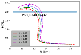
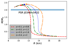
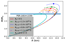
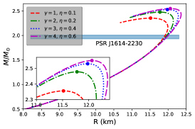
Figure 5: Variation of stellar mass $M/M_{\odot}$ with stellar radius $R$. Solid circles represent the maximum-mass star of each stellar sequence. Here, upper panels feature NS $M/M_{\odot}$ vs. $R$ for (i) varying $B_{0}$ and $\kappa=0.5$ (upper left), (ii) varying $\kappa$, where $B_{0}=6\times{10}^{17}$ G (upper middle) and (iii) varying $\eta$ and $\gamma$, where $B_{0}=6\times{10}^{17}$ G and $\kappa=0.5$ (upper right). However, lower panels feature SQS $M/M_{\odot}$ vs. $R$ for (i) varying $B_{0}$, where $\kappa=0.5$ (lower left), (ii) varying $\kappa$, where $B_{0}=2.4\times{10}^{18}$ G (lower middle) and (iii) varying $\eta$ and $\gamma$, where $B_{0}=1.2\times{10}^{18}$ G and $\kappa=0.5$ (lower right).

3 Results and discussions

In the present article, we study compact stellar objects, viz., NSs and SQSs with strong magnetic fields, assuming that they are approximately spherically symmetric. Importantly, we show that not only the magnetic field strength and anisotropy have a significant effect on the stellar configurations, but that also the orientation of the magnetic field (viz., RO or TO) has a pronounced, non-negligible influence on the stars, too.

To describe NSs and SQSs we assume that their interiors can reasonably well be described by SLy EOS and the MIT bag model EOS, respectively. Further, to close the system of equations, we assume a functional form for the anisotropy that is shown in Eq. (14). Finally, following Bandyopadhyay et al. (1997, 1998) we consider density dependent magnetic field strength profiles for NSs and SQSs which are given by Eqs. (16) and (17). When presenting the results of our study, we have chosen pulsars PSR J0348+0432 and PSR J1614$-$2230 as reference stars. The observed masses of these stars are $2.01\pm 0.04~{}M_{\odot}$ (Antoniadis et al., 2013) and $1.97\pm 0.04~{}M_{\odot}$ (Demorest et al., 2010), respectively. To study NSs we have chosen $B_{s}=10^{13}$ G and $B_{0}$ as $0.9\times{10}^{18}$ G and $1.2\times{10}^{18}$ G for TO, and $6\times{10}^{17}$ G and $9\times{10}^{17}$ G for RO. For the SQSs, we choose $B_{s}=10^{15}$ G and $B_{0}$ as $1.2\times{10}^{17}$ G and $2.4\times{10}^{17}$ G for TO, and $0.8\times{10}^{17}$ G and $1.1\times{10}^{17}$ G for RO. Note that the choice of the values of $B_{0}$ is not same for TO and RO as well as those between NS and SQS. This is because the effects on stellar mass by the magnetic field are different between TO and RO magnetic fields. For both types of stars we assume $\kappa=0.5$ as a reference value. For SQSs we assume a bag constant value of $\mathcal{B}=60~{}\mathrm{MeV/{fm^{3}}}$, which describes SQM that is strongly bound with respect to nuclear matter.

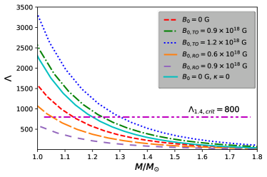
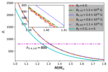
Figure 6: Variation of tidal deformability $\Lambda$ with respect to stellar mass $M/M_{\odot}$ for various $B_{0}$ and $\kappa=0.5$. In the upper and lower panels we present cases for NSs and SQSs respectively.

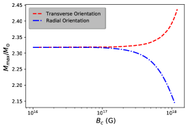
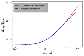
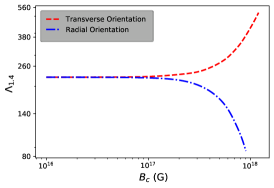
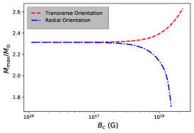
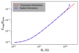
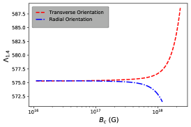
Figure 7: Variation of (i) stellar maximum mass $M_{max}$  (left panels), (ii) ratio of magnetic energy $E_{mag}$ to gravitational energy $E_{grav}$ (middle panels) and (iii) tidal deformability ($\Lambda_{1.4}$) for $1.4~{}M_{\odot}$ star (right panels) with central magnetic field strength $B_{c}$. In the upper and lower panels, we present cases for NSs and SQSs, respectively.

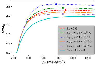
Figure 8: $M/M_{\odot}$ as a function of the matter central matter density $\rho_{c}$ for NSs and SQSs in the left and right panels, respectively. Solid circles represent the maximum mass stars of each stellar sequence.

The profiles for the matter density $\rho$ from the center to the surface with the normalized radial coordinate $r/R$, where $R$ is the stellar radius, are shown for NS and SQS in the left and right upper panels of Figure 1, respectively, for different parametric values of $B_{0}$. The corresponding profiles for the radial matter pressure $p_{r}$ are featured in the left and right middle panels of Figure 1 for NSs and SQSs, respectively. Similarly, the variations of the tangential matter pressure $p_{t}$ is shown in the left and right bottom panels of Figure 1. Clearly, Figure 1 shows that $\rho$, $p_{r}$ and $p_{t}$ have finite maximum values at the core of the stellar system and then decrease gradually to attain their respective minimum values at the surface, which ensures physical stability of the achieved solutions. Figure 1 also confirms that the present model is free from any sort of singularities at the core of the system. Figure 2 shows the effects of the magnetic field on the EOSs of the compact stellar objects. In the upper and lower panels of Figure 2 we present the variations of the system parallel pressure $p_{\parallel}$ and transverse pressure $p_{\bot}$ with the system density $(\widetilde{\rho})$, normalized to the system central density $(\widetilde{\rho}_{c})$, for NSs and SQSs, respectively. Interestingly, our study reveals that as the magnetic field strength increases, the system pressures of the compact stars gradually become stiffer for RO, whereas they gradually become softer for TO, which is evident in Figure 2. Importantly, at the center for each of the cases, $p_{\parallel}$ and $p_{\bot}$ have the same value which ensures zero anisotropy at the stellar core. The variation of anisotropy, due to both the local anisotropy of the fluid and the presence of a strong magnetic field, is shown in Figure 3. Importantly, in the upper and lower panels of Figure 3 one sees that the anisotropy at the center of both NSs and SQSs is zero, which ensures hydrodynamic stability of the system via the balance of the forces. It is worth mentioning that as long as the anisotropy is considered only due to the presence of a strong magnetic field, the anisotropic force shows attractive nature if the field is in TO, whereas the same force is repulsive for RO fields. Hence, within the stars, the slopes of the anisotropy profiles gradually increase for TO as $B_{0}$ increases, whereas they gradually decrease with increasing $B_{0}$ for RO magnetic fields. Furthermore, the profiles for the density dependent magnetic fields inside NSs and SQSs are featured in the upper and lower panels of Figure. 4, respectively, which show that the magnetic field is maximum at the core of these stars and decreases monotonically throughout their interiors to reach their minimum values at the surface.

To shed light on the widely unknown hadronic EOS in the high-density regime it is important to study the mass-radius relationship of compact stars, which allows one to rule out or support existing models of hadronic EOSs. In the present work, the study of the mass-radius relation is used to analyse the effects of strong magnetic fields, their orientations and anisotropy on compact stellar configurations and to control their properties. In the upper and lower left panels of Figure 5, we show mass-radius relations for NSs and SQSs, respectively, for a range of different $B_{0}$ values. The mass-radius relations for NSs and SQSs due to varying $\kappa$ values are shown in the upper and lower middle panels of Figure. 5, respectively. The upper and lower right panels of Figure 5 show the mass-radius relations due to different parametric choices of $\eta$ and $\gamma$ for NSs and SQSs, respectively. From the upper left panel of Figure 5 one sees that for TO magnetic fields and $B_{0}=1.2\times{10}^{18}$ G the maximum mass and corresponding radius of the NSs increase by 5.09% and 12.09%, respectively, compared to the anisotropic but non-magnetized case. The maximum mass and associated radius increase to 18.75% and 17.95%, respectively, in comparison to the isotropic non-magnetized case.

However, for the RO case with $B_{0}=0.9\times{10}^{18}$ G the maximum mass and associated radius of NSs decrease by 5.47% and 9.49%, respectively, compared to the anisotropic but non-magnetized case. But compared to their values in the isotropic non-magnetized case, the maximum mass increases by 6.82% while the corresponding radius decreases by 4.75%. the upper middle, upper right, lower middle and lower right panels of Figure 5 show that the maximum mass and its corresponding radius increase gradually for both NSs and SQSs when the values of $\kappa$, $\eta$ and $\gamma$ gradually increase. The lower left panel of Figure 5 shows that for $B_{0}=2.4\times{10}^{18}$ G and the TO field, the maximum mass and the corresponding radius increase by 13.74% and 2.20%, respectively, compared to anisotropic but non-magnetized SQSs. On the other hand, these values increase by 8.31% and 9.48%, respectively, compared to the isotropic and non-magnetized case. For the RO case, however, for $B_{0}=1.1\times{10}^{18}$ G the maximum mass of SQSs and the corresponding radius decrease by 9.16% and 1.62%, respectively, compared to the anisotropic but non-magnetized case. With respect to the isotropic and non-magnetized SQSs, these values decrease by 6.92% and 5.39%, respectively.

In Figure 6 we present the compatibility of our model with respect to the tidal deformability ($\Lambda$) for both NSs and SQSs, constrained from the observation of GW emission related to GW170817 event, detected by the LIGO/Virgo Collaboration (LVC) (Abbott et al., 2017, 2018, 2019). The investigation by LVC sets an upper limit of $\Lambda$ associated with $1.4M_{\odot}$ pulsars ($\Lambda_{1.4}$) by Abbott et al. (2017) which is given as $\Lambda_{1.4}<800$ for the low-spin cases. In the upper and lower panels of Figure 6, we show the variation of $\Lambda$ with respect to $M$ for both NSs and SQSs, respectively, for various $B_{0}$ and $\kappa=0.5$. Evidently, for both the cases, $\Lambda_{1.4}$ lies well below its critical value, which confirms the physical validity of the assumed EOSs, viz., SLy and MIT bag model EOSs for NSs and SQSs, respectively. In Figure 6, one may also notice that $\Lambda$ increases with increasing $B_{0}$ for TO, whereas it decreases with increasing $B_{0}$ for RO.

In Figure 7 we present the effect of magnetic field orientation on the physical properties of both the stars, such as $M_{max}$, the ratio of magnetic to gravitational energies and tidal deformability for $1.4~{}M_{\odot}$ stars. Although the masses of NSs and SQSs increase or decrease (based on the orientation of the magnetic field) compared to their values in the anisotropic and non-magnetized cases, they change asymmetrically, which is shown in the upper left and lower left panels of Figure 7. From the upper left panel of Figure 7, one sees that for $B_{0}={10}^{18}$ G and $\kappa=0.5$ the maximum masses of NSs are $2.39~{}M_{\odot}$ for the TO case and $2.17~{}M_{\odot}$ for the RO case, which leads to a 10.38% asymmetry in the masses. Similarly, the lower left panel of Figure 7 reveals that for $B_{0}=1.5\times{10}^{18}$ G and $\kappa=0.5$, the maximum masses of SQSs are $2.48~{}M_{\odot}$ and $1.73~{}M_{\odot}$ for TO and RO cases, respectively, which leads to $42.91\%$ asymmetry in the masses. Evidently, for both the stars, as the central magnetic field $B_{c}$ increases, the effects of magnetic field orientations via mass-asymmetry become larger gradually, which corroborate the conclusion of Chu et al. (2014) that orientations of the magnetic field have a significant effect on the maximum mass of magnetized compact stars. Further, the left upper and lower panels of Figure 7 exhibit that for $B_{c}<10^{17}$ G, the anisotropic compact stars are not sensitive to the present magnetic field strength and their orientations within the stars. Again, note that Sinha et al. (2013) showed for the magnetic field strength less than $3\times 10^{18}$ G, the effects of Landau quantization are not considerable within the magnetized compact stars. We therefore choose to constrain $B_{c}$ in our work as $10^{17}$ G$<B_{c}<3\times 10^{18}$ G. In the right upper and lower panels of Figure 7, we also show the effect of magnetic field orientation on $\Lambda_{1.4}$, which increases with increasing $B_{c}$ for the TO case and decreases with increasing $B_{c}$ for the RO case. Chu et al. (2021) found the same dependency of $\Lambda_{1.4}$ on the magnetic field orientations which confirms our results in the case of anisotropic magnetized compact stars. Hence, through this work, we explore that for anisotropic magnetized stars, anisotropy, magnetic field strength and orientations of the magnetic field have a significant effect on $\Lambda_{1.4}$. Hence, RO and TO cases of the magnetic field play a significant role in magnetized stellar configurations.

Chandrasekhar & Fermi (1953) found that in the case of magnetized relativistic stars, instead of $\Gamma>\frac{4}{3}$ the system may be dynamically unstable due to a sufficiently strong internal magnetic field, which may induce dynamical instability in compact stars. They found that in magnetized stars, the necessary condition to achieve a stellar equilibrium configuration is $\mid E_{grav}\mid>E_{mag}$, where $E_{grav}$ and $E_{mag}$ are the gravitational potential energy and magnetic energy, respectively. In the middle upper and lower panels of Figure 7 we show that for both NS and SQS, respectively, $E_{grav}$ dominates significantly over $E_{mag}$ for both orientations of the magnetic field, which confirms the dynamic stability of these magnetized compact stellar objects. Further to discuss the stability of a spherically symmetric static stellar structure, the model must be consistent with the condition $\mathrm{d}M/\mathrm{d}\rho_{c}>0$, say, up to the maximum mass (Harrison et al., 1965). From the left and right panels of Figure 8, it is evident that both NSs and SQSs fulfill this stability criterion.

Further, we check the absolutely stable condition for both the EOSs of NSs and SQSs. We find the minimum energy per baryon for SQM is less than 930 MeV for the chosen values of $B_{0}$ in the case of MIT bag model EOS. On the other hand, the minimum energy per baryon for NS matter described by SLy EOS is greater than 930 MeV for the chosen values of $B_{0}$. In Figure 9, we show the variation of the energy per baryon with the ratio of baryon number density ($n_{b}$) to its maximum value ($n_{max}$), which also confirms that SQM may be the true ground state for strong interactions.

We also examine the sound speed ($c_{s}$) for all the cases due to NS. We find that the sound speeds for NS are well within the causality limit for different $B_{0}$ as shown in Figure 10. Since we use MIT bag model EOS to describe SQM distribution within SQS, $c_{s}$ for SQS is always given by $c_{s}=\sqrt{d{p_{r}}/d\rho}=\sqrt{1/3}\sim 0.58$. Therefore, in this work, the causality condition does not violate for any chosen EOSs with or without strong magnetic fields.

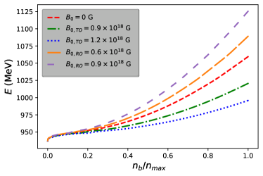
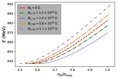
Figure 9: Variation of energy per baryon ($E$) with the ratio of baryon number density ($n_{b}$) to the maximum value of $n_{b}$ ($n_{max}$) for various $B_{0}$ and $\kappa=0.5$. In the upper and lower panels we present cases for NSs and SQSs, respectively.

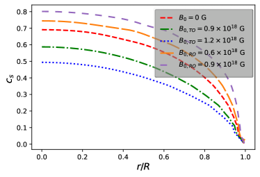
Figure 10: Variation of sound speed $(c_{s})$ with radial coordinate $r/R$ for $2.01\pm 0.04~{}M_{\odot}$ (Antoniadis et al., 2013) NS candidate PSR J0348+0432.

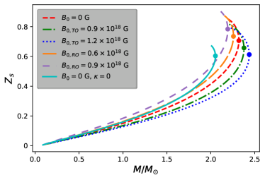
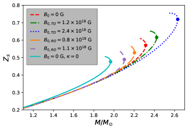
Figure 11: Variation of surface redshift $(Z_{s})$ with $M/M_{\odot}$ for NSs (upper panel) and SQSs (lower panel).

For a better understanding of the effects due to anisotropy, the role of magnetic fields and their orientations, in Tables 1, 2, 3 and 4 we present numerical values of different stellar properties, viz., maximum mass, the corresponding radius, $B_{c}$, $\widetilde{\rho}_{c}$, $\widetilde{p}_{c}$, Buchdahl ratio, surface redshift ($Z_{s}$), the ratio of magnetic energy ($E_{mag}$) to gravitational energy ($E_{grav}$) and $\Lambda_{1.4}$ for NSs and SQSs. One sees from Tables 1 and 3 that for TO magnetic fields the maximum mass and the corresponding radius increase with increasing values of $B_{0}$, whereas for RO magnetic fields the maximum mass and the corresponding radius decrease gradually with increasing values of $B_{0}$. On the other hand, Tables 2 and 4 show that the mass and the radius of a star increases if the strength of the anisotropy, $\kappa$, is increased. For all cases, the value of $2M/R$ lies well below the critical value of $8/9$. In Tables 1-4 we also demonstrate that in each case, $\mid E_{grav}\mid$ is significantly higher than $E_{mag}$, which confirms stability of these stars (Chandrasekhar & Fermi, 1953). In Figure 11 we show the variation of the surface redshift with mass, for TO and RO magnetic fields and different values of $B_{0}$. Numerical values of the surface redshifts of maximum-mass stars for different cases are listed in Tables 1-4. We also show in Tables 1-4 that in each case tidal deformability for $1.4~{}M_{\odot}$ star is well bellow the critical value $\Lambda_{1.4,crit}=800$.

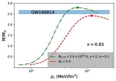
Figure 12: Variation of the total mass of the NSs in the units of Solar mass $(M/M_{\odot})$ with the matter central density $\rho_{c}$. Here, we choose $\kappa=0.65$.

From the mass-radius relations shown in Figure 5 and the data provided in Tables 1-4, the following general conclusions can be drawn. As $B_{0}$ increases in compact stars with TO magnetic fields, the anisotropic and magnetized stellar objects become more massive and larger due to the gradual increase of the repulsive, effectively anisotropic and Lorentz forces. The stars become also more massive and larger if the strength of the anisotropy, $\kappa$, increases. On the contrary, the stars with RO magnetic fields become less massive and smaller in size for gradually increasing values of the magnetic field, since the corresponding effective anisotropic force simultaneously decreases. Interestingly, we point out that anisotropic, magnetized compact stars can have masses that are in the mass range $2.50-2.67~{}M_{\odot}$ deduced for the lighter companion in the binary compact-object coalescence event GW190814, observed recently by LIGO and Virgo (Abbott et al., 2020), as shown in Figure 12. With the appropriate choice of the physical parameters, such as $B_{0}=2.4\times{10}^{18}$ G, $\eta=0.1$, $\gamma=2$ and $\kappa=0.65$, we find that the maximum possible mass of a NS is $\sim 2.79~{}M_{\odot}$, which comfortably accommodates the anomalously high mass of the lighter object associated with GW190814. We note that by considering rotation of the anisotropic and magnetized stars in a future study, the maximum mass of a NS will be pushed to even higher values.

Table 1: Numerical values of physical parameters for the NSs with $\kappa=0.5$ for different values of $B_{0}$

Orientation	Value	Value of	Corresponding	Central	Central	Central		Surface
of Magnetic	of $B_{0}$	Maximum	Predicted	Magnetic field	Density	Pressure	$\frac{2M}{R}$	Redshift	$\frac{E_{mag}}{E_{grav}}$	$\Lambda_{1.4}$
field	(Gauss)	Mass $(M_{\odot})$	Radius (km)	$B_{c}$ (Gauss)	$\widetilde{\rho}_{c}~{}(\rm g/{cm}^{3})$	$\widetilde{p}_{c}~{}(\rm dyne/{cm}^{2})$		$(Z_{s})$
TO	$1.2\times{10}^{18}$	$2.438$	$11.685$	$1.2\times{10}^{18}$	$1.891\times{10}^{15}$	$6.316\times{10}^{35}$	$0.62$	$0.61$	$0.088$	$523.17$
	$0.9\times{10}^{18}$	$2.378$	$11.030$	$0.9\times{10}^{18}$	$2.117\times{10}^{15}$	$7.838\times{10}^{35}$	$0.64$	$0.66$	$0.043$	$388.44$
$B=0$	-	$2.320$	$10.425$	-	$2.295\times{10}^{15}$	$9.120\times{10}^{35}$	$0.66$	$0.71$	-	$225.90$
RO	$0.6\times{10}^{18}$	$2.258$	$9.975$	$0.6\times{10}^{18}$	$2.465\times{10}^{15}$	$1.020\times{10}^{36}$	$0.67$	$0.73$	$0.015$	$149.11$
	$0.9\times{10}^{18}$	$2.193$	$9.436$	$0.9\times{10}^{18}$	$2.736\times{10}^{15}$	$1.209\times{10}^{36}$	$0.69$	$0.78$	$0.029$	$86.29$

Table 2: Numerical values of physical parameters for the NSs with $B_{0}=0.9\times{10}^{18}$ for different values of $\kappa$

Value	Value of	Corresponding	Central	Central	Central		Surface
of $\kappa$	Maximum	Predicted	Magnetic field	Density	Pressure	$\frac{2M}{R}$	Redshift	$\frac{E_{mag}}{E_{grav}}$	$\Lambda_{1.4}$
	Mass $(M_{\odot})$	Radius (km)	$B_{c}$ (Gauss)	$\widetilde{\rho}_{c}~{}(\rm g/{cm}^{3})$	$\widetilde{p}_{c}~{}(\rm dyne/{cm}^{2})$		$(Z_{s})$
$0.15$	$2.179$	$10.698$	$9.000\times{10}^{17}$	$2.406\times{10}^{15}$	$9.715\times{10}^{35}$	$0.60$	$0.58$	$0.0428$	$423.41$
$0.30$	$2.260$	$10.860$	$9.000\times{10}^{17}$	$2.257\times{10}^{15}$	$8.880\times{10}^{35}$	$0.61$	$0.61$	$0.0431$	$392.41$
$0.45$	$2.347$	$11.031$	$9.000\times{10}^{17}$	$2.117\times{10}^{15}$	$7.838\times{10}^{35}$	$0.63$	$0.64$	$0.0434$	$385.45$
$0.60$	$2.443$	$11.210$	$9.000\times{10}^{17}$	$1.986\times{10}^{15}$	$6.257\times{10}^{35}$	$0.64$	$0.67$	$0.0438$	$395.52$

Table 3: Numerical values of physical parameters for the SQSs with $\kappa=0.5$ and $\mathcal{B}=60~{}\mathrm{MeV/{fm^{3}}}$ for different values of $B_{0}$

Orientation	Value	Value of	Corresponding	Central	Central	Central		Surface
of Magnetic	of $B_{0}$	Maximum	Predicted	Magnetic field	Density	Pressure	$\frac{2M}{R}$	Redshift	$\frac{E_{mag}}{E_{grav}}$	$\Lambda_{1.4}$
field	(Gauss)	Mass $(M_{\odot})$	Radius (km)	$B_{c}$ (Gauss)	$\widetilde{\rho}_{c}~{}(\rm g/{cm}^{3})$	$\widetilde{p}_{c}~{}(\rm dyne/{cm}^{2})$		$(Z_{s})$
TO	$2.4\times{10}^{18}$	$2.632$	$11.730$	$2.296\times{10}^{18}$	$1.610\times{10}^{15}$	$4.939\times{10}^{35}$	$0.66$	$0.72$	$0.33$	$587.91$
	$1.2\times{10}^{18}$	$2.423$	$11.585$	$1.185\times{10}^{18}$	$1.603\times{10}^{15}$	$3.892\times{10}^{35}$	$0.62$	$0.62$	$0.09$	$577.33$
$B=0$	-	$2.314$	$11.477$	-	$1.609\times{10}^{15}$	$3.537\times{10}^{35}$	$0.59$	$0.57$	-	$575.32$
RO	$0.8\times{10}^{18}$	$2.203$	$11.367$	$7.931\times{10}^{17}$	$1.609\times{10}^{15}$	$3.204\times{10}^{35}$	$0.57$	$0.53$	$0.04$	$573.98$
	$1.1\times{10}^{18}$	$2.102$	$11.291$	$1.086\times{10}^{18}$	$1.593\times{10}^{15}$	$2.864\times{10}^{35}$	$0.55$	$0.49$	$0.08$	$572.28$

Table 4: Numerical values of physical parameters for the SQSs with $B_{0}=2.4\times{10}^{18}$ G and $\mathcal{B}=60~{}\mathrm{MeV/{fm^{3}}}$, for different values of $\kappa$

Value	Value of	Corresponding	Central	Central	Central		Surface
of $\kappa$	Maximum	Predicted	Magnetic field	Density	Pressure	$\frac{2M}{R}$	Redshift	$\frac{E_{mag}}{E_{grav}}$	$\Lambda_{1.4}$
	Mass $(M_{\odot})$	Radius (km)	$B_{c}$ (Gauss)	$\widetilde{\rho}_{c}~{}(\rm g/{cm}^{3})$	$\widetilde{p}_{c}~{}(\rm dyne/{cm}^{2})$		$(Z_{s})$
$0.15$	$2.365$	$11.297$	$2.381\times{10}^{18}$	$1.853\times{10}^{15}$	$5.775\times{10}^{35}$	$0.62$	$0.62$	$0.3280$	$478.50$
$0.30$	$2.473$	$11.474$	$2.357\times{10}^{18}$	$1.748\times{10}^{15}$	$5.430\times{10}^{35}$	$0.64$	$0.66$	$0.3285$	$520.49$
$0.45$	$2.590$	$11.673$	$2.308\times{10}^{18}$	$1.631\times{10}^{15}$	$5.017\times{10}^{35}$	$0.65$	$0.70$	$0.3302$	$567.95$
$0.60$	$2.718$	$11.881$	$2.238\times{10}^{18}$	$1.530\times{10}^{15}$	$4.629\times{10}^{35}$	$0.67$	$0.75$	$0.3319$	$629.68$

4 Prospects of future work on white dwarfs

In their recent study, Chowdhury & Sarkar (2019) attempted to explain white dwarfs (WDs) based on an anisotropic spherically-symmetric model in the framework of modified gravity theory and indicated the possible existence of super-Chandrasekhar WDs beyond the standard Chandrasekhar mass limit. It is worth mentioning that during the last few years Mukhopadhyay and collaborators (Das & Mukhopadhyay, 2012, 2013; Vishal & Mukhopadhyay, 2014; Das & Mukhopadhyay, 2015a; Subramanian & Mukhopadhyay, 2015; Mukhopadhyay & Rao, 2016; Mukhopadhyay et al., 2017; Bhattacharya et al., 2018; Kalita & Mukhopadhyay, 2018, 2019) through their series of important works have established the possible existence of highly super-Chandrasekhar mass WDs. They found that the presence of a strong magnetic field leads to super-Chandrasekhar WDs which suitably served as a progenitor of the peculiar overluminous type Ia supernovae (SNeIa). Although in this article, we mainly focus on ultra-dense compact stars it will be interesting to investigate the effects of anisotropy, strong magnetic fields and the orientation of the magnetic field on WDs. The upper limit of density for these highly magnetized WDs (B-WDs) is constrained by the effects of electron capture and pycnonuclear fusion reactions (Otoniel et al., 2019). In Figure 13 we demonstrate that inclusion of anisotropy and TO of the magnetic field increases the maximum mass of B-WDs compared to the non-magnetized isotropic case, whereas in the case of a RO of the magnetic field the maximum mass of B-WDs drops compared to the non-magnetized anisotropic case. Although, we take the opportunity to discuss whether the present model can suitably explain anisotropic B-WDs, the understanding of their properties requires a detailed discussion which is beyond the scope of this study. We are going to report it in our next work, which is in progress.

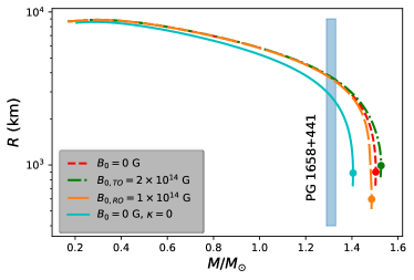
Figure 13: Mass-radius relations of white dwarfs for different magnetic field strengths. Solid circles represent the maximum mass star of each stellar sequence.

5 Conclusion

In this work, we study the combined effects of anisotropy, strong magnetic fields and their orientations on the properties of spherically symmetric compact objects, viz., NSs and SQSs. Our study reveals that in a magnetized compact stellar object the magnetic field strength, the orientation of the magnetic field and the anisotropy influence the EOS of the system by modifying both the matter and pressures of the system. Although in the present study we consider spherically symmetric compact objects, one may point out that the occurrence of anisotropy may push the system toward non-spherical symmetry. However, it is already known that for a toroidally dominated field magnetized stars exhibit negligible deviations from spherical symmetry (Das & Mukhopadhyay, 2015b; Subramanian & Mukhopadhyay, 2015; Kalita & Mukhopadhyay, 2019). For example, the maximum value of anisotropy in the case of TO magnetic fields with $B_{0}=1.2\times{10}^{18}$ G in a NS is $\sim 80\%$ lower than $p_{c}$ (see the upper panel of Figure 3), and for $B_{0}=2.4\times{10}^{18}$ G in a SQS it is $\sim 81\%$ lower than $p_{c}$ (see the lower panel of Figure 3). This indicates that treating magnetized anisotropic stars as spherically symmetric objects has no considerable influence on the geometry of the stellar configurations.

Ferrer et al. (2010) showed that inclusion of a strong magnetic field invites anisotropy within the system due to the distinction between parallel and transverse pressures. However, it is also important for such anisotropic and magnetized stars that they are consistent with the TOV equations throughout the stars, which ensures hydrostatic stability of the systems via equilibrium of forces. Nevertheless, to the best of our knowledge, prior to this study, the issue of non-zero value of anisotropic force in the center of highly magnetized compact stars mostly remained unnoticed. One may easily check via the TOV equations (see Eq. 13) that the non-zero value of anisotropy at the center leads to instability due to non-equilibrium of the forces. On the other hand, the anisotropy which originates due to the presence of the strong magnetic field via the distinction between the parallel and transverse pressures, which is $\sim\mid B^{2}\mid$, cannot be zero at the center due to the maximum finite value of the magnetic field at the stellar core. Interestingly, we find that this situation can be taken care of by considering the anisotropic effect due to both the local anisotropy of the fluid and the presence of the strong magnetic field.

Of course, the present study offers only a simplified treatment of the complex structure of magnetised compact stellar configurations. But through our work, we are able to demonstrate that to study magnetised compact stars, it is essential to consider the effective anisotropies of both the fluid and the magnetic field, which have a significant influence on the properties of compact stars. Based on the orientation of the magnetic field, the maximum mass of static magnetized compact stars may be enhanced or reduced, which resolves the long-standing issue whether or not the mass of the system increases or decreases due to the presence of a strong magnetic field. Importantly, the present study has also explored the magneto-hydrostatic stability of the system, which demonstrates the physical validity of this model.

6 acknowledgments

Research of D. D. is funded by the C. V. Raman Postdoctoral Fellowship (Reg. No. R(IA)CVR-PDF/2020/222) from Department of Physics, Indian Institute of Science. F. W. is supported through the U.S. National Science Foundation under Grants PHY-1714068 and PHY-2012152. This work is partly supported by a fund of Department of Science and Technology (DST-SERB) with research Grant No. DSTO/PPH/BMP/1946 (EMR/2017/001226). One of the authors (D. D.) is thankful to Surajit Kalita of IISc for his pertinent suggestions which helped to upgrade the paper. We are also thankful to the referee for their pertinent comments, which helped us in upgrading our work substantially. All computations were performed in open source softwares, and the authors are sincerely thankful to the open source community.

References

- Abbott et al. (2017) Abbott, B. P., Abbott, R., Abbott, T. D., et al. 2017, Phys. Rev. Lett., 119, 161101.
- Abbott et al. (2018) Abbott, B. P., Abbott, R., Abbott, T. D., et al. 2018, Phys. Rev. Lett., 121, 161101.
- Abbott et al. (2019) Abbott, B. P., Abbott, R., Abbott, T. D., et al. 2019, Physical Review X, 9, 011001.
- Abbott et al. (2020) Abbott, R., Abbott, T. D., Abraham, S., et al. 2020, ApJ, 896, L44.
- Abrahams & Shapiro (1991) Abrahams, A. M. & Shapiro, S. L. 1991, ApJ, 374, 652.
- Alaverdyan & Vartanyan (2017) Alaverdyan, G. B. & Vartanyan, Y. L. 2017, Astrophysics, 60, 563.
- Alcock et al. (1986) Alcock, C., Farhi, E., & Olinto, A. 1986, ApJ, 310, 261.
- Alcock & Olinto (1988) Alcock, C. & Olinto, A. 1988, Annual Review of Nuclear and Particle Science, 38, 161.
- Alpar et al. (1982) Alpar, M. A., Cheng, A. F., Ruderman, M. A., et al. 1982, Nature, 300, 728.
- Aguirre (2020) Aguirre, R. M. 2020, Phys. Rev. D, 102, 096025.
- Arbañil & Malheiro (2016) Arbañil, J. D. V. & Malheiro, M. 2016, J. Cosmology Astropart. Phys, 2016, 012.
- Antoniadis et al. (2013) Antoniadis, J., Freire, P. C. C., Wex, N., et al. 2013, Science, 340, 448.
- Bandyopadhyay et al. (1997) Bandyopadhyay, D., Chakrabarty, S., & Pal, S. 1997, Phys. Rev. Lett., 79, 2176.
- Bandyopadhyay et al. (1998) Bandyopadhyay D., Chakrabarty S., Dey P., Pal S., 1998, PhRvD, 58, 121301.
- Bandyopadhyay et al. (1998) Bandyopadhyay, D., Pal, S., & Chakrabarty, S. 1998, Journal of Physics G Nuclear Physics, 24, 1647.
- Barreto & Rojas (1992) Barreto, W. & Rojas, S. 1992, Ap&SS, 193, 201.
- Barreto (1993) Barreto, W. 1993, Ap&SS, 201, 191.
- Baruah Thapa et al. (2020) Baruah Thapa, V., Sinha, M., Li, J.-J., et al. 2020, Particles, 3, 660.
- Bayin (1982) Bayin, S. S. 1982, Phys. Rev. D, 26, 1262.
- Bocquet et al. (1995) Bocquet, M., Bonazzola, S., Gourgoulhon, E., et al. 1995, A&A, 301, 757 (BB95).
- Bodmer (1971) Bodmer, A. R. 1971, Phys. Rev. D, 4, 1601.
- Bombaci et al. (2004) Bombaci, I., Parenti, I., & Vidaña, I. 2004, ApJ, 614, 314.
- Bordbar et al. (2012) Bordbar, G. H., Bahri, H., & Kayanikhoo, F. 2012, Research in Astronomy and Astrophysics, 12, 1280.
- Bowers & Liang (1974) Bowers, R. L. & Liang, E. P. T. 1974, ApJ, 188, 657.
- Broderick et al. (2000) Broderick, A., Prakash, M., & Lattimer, J. M. 2000, ApJ, 537, 351.
- Burgio et al. (2002) Burgio, G. F., Baldo, M., Sahu, P. K., et al. 2002, Phys. Rev. C, 66, 025802.
- Cameron & Canuto (1974) Cameron, A. G. W. & Canuto, V. 1974, Astrophysics and Gravitation, 221.
- Canuto (1974) Canuto, V. 1974, ARA&A, 12, 167.
- Canuto (1977) Canuto, V. 1977, Eighth Texas Symposium on Relativistic Astrophysics, 302, 514.
- Canuto & Ventura (1977) Canuto, V. & Ventura, J. 1977, Fund. Cosmic Phys., 2, 203.
- Cardall et al. (2001) Cardall, C. Y., Prakash, M., & Lattimer, J. M. 2001, ApJ, 554, 322.
- Carter & Langlois (1998) Carter, B. & Langlois, D. 1998, Nuclear Physics B, 531, 478.
- Casali et al. (2014) Casali, R. H., Castro, L. B., & Menezes, D. P. 2014, Phys. Rev. C, 89, 015805.
- Cenko et al. (2010) Cenko, S. B., Frail, D. A., Harrison, F. A., et al. 2010, ApJ, 711, 641.
- Chaichian et al. (2000) Chaichian, M., Masood, S. S., Montonen, C., et al. 2000, Phys. Rev. Lett., 84, 5261.
- Chaisi & Maharaj (2005) Chaisi, M. & Maharaj, S. D. 2005, General Relativity and Gravitation, 37, 1177.
- Chakarabarty (1994) Chakarabarty, S. 1994, Ap&SS, 213, 121. doi:10.1007/BF00627782
- Chakrabarty (1996) Chakrabarty, S. 1996, Phys. Rev. D, 54, 1306.
- Chakrabarty et al. (1997) Chakrabarty, S., Bandyopadhyay, D., & Pal, S. 1997, Phys. Rev. Lett., 78, 2898.