Multi-Dimensional Radiative Transfer Calculations of Double Detonations of Sub-Chandrasekhar-Mass White Dwarfs

Abstract

Study of the double detonation Type Ia supernova scenario, in which a helium shell detonation triggers a carbon core detonation in a sub-Chandrasekhar-mass white dwarf, has experienced a resurgence in the past decade. New evolutionary scenarios and a better understanding of which nuclear reactions are essential have allowed for successful explosions in white dwarfs with much thinner helium shells than in the original, decades-old incarnation of the double detonation scenario. In this paper, we present the first suite of light curves and spectra from multi-dimensional radiative transfer calculations of thin-shell double detonation models, exploring a range of white dwarf and helium shell masses. We find broad agreement with the observed light curves and spectra of non-peculiar Type Ia supernovae, from subluminous to overluminous subtypes, providing evidence that double detonations of sub-Chandrasekhar-mass white dwarfs produce the bulk of observed Type Ia supernovae. Some discrepancies in spectral velocities and colors persist, but these may be brought into agreement by future calculations that include more accurate initial conditions and radiation transport physics.

1 Introduction

The identity of Type Ia supernova (SN Ia) progenitors remains uncertain. There is general consensus that these explosions are powered by the radioactive decay of ⁵⁶Ni (Pankey, 1962; Colgate & McKee, 1969) produced in the explosion of a white dwarf (WD), but the mechanism of the explosion and the nature of the companion(s) are still debated (for a review, see Maoz et al. 2014).

A double detonation of a sub-Chandrasekhar-mass WD, in which a helium shell detonation triggers a carbon core detonation, was one of the first proposed SN Ia mechanisms (e.g., Nomoto, 1982; Woosley et al., 1986). However, the model fell out of favor due to discrepancies with observed SNe Ia imparted by the thermonuclear ash from the relatively massive ($\sim 0.1\,M_{\sun}$) helium shells that arise when the donor is a low-mass, non-degenerate helium star (Höflich & Khokhlov, 1996; Nugent et al., 1997).

More recently, there has been a resurgence in research into this SN Ia explosion mechanism due in part to the realization that the helium shells at the onset of the supernova in double WD binary progenitors are orders of magnitude smaller than previously considered (Bildsten et al., 2007; Guillochon et al., 2010; Dan et al., 2012; Raskin et al., 2012), yet are still massive enough to support successful shell and subsequent core detonations (Townsley et al., 2012; Moore et al., 2013; Shen & Bildsten, 2014; Shen & Moore, 2014). These theoretical studies have been further bolstered by the observational confirmation that double WD binaries definitively lead to sub-Chandrasekhar-mass WD explosions that are likely SNe Ia (Shen et al., 2018b). The combination of theoretical and observational motivation has led to a large number of explosion and radiative transfer simulations of sub-Chandrasekhar-mass WD detonations, with a range of physical configurations, dimensionality, nuclear reaction network complexity, and radiation transport approximations (e.g., Fink et al., 2007, 2010; Kromer et al., 2010; Pakmor et al., 2010, 2011, 2012, 2013, 2021; Sim et al., 2010, 2012; Kushnir et al., 2013; Moll & Woosley, 2013; Moll et al., 2014; Raskin et al., 2014; Blondin et al., 2017; Shen et al., 2018a, 2021; Tanikawa et al., 2018, 2019; Miles et al., 2019; Polin et al., 2019, 2021; Townsley et al., 2019; Leung & Nomoto, 2020; Gronow et al., 2020, 2021; Boos et al., 2021; Magee et al., 2021). Of these, Townsley et al. (2019) was the first study of a multi-dimensional explosion simulation utilizing a large enough reaction network to allow for a very thin ($0.02\,M_{\sun}$ on a $1.0\,M_{\sun}$ core) helium shell detonation. Townsley et al. (2019)’s work was subsequently expanded upon by Boos et al. (2021)’s study of a range of thin-shell explosion models.

In this paper, we follow-up Boos et al. (2021)’s work and present the first suite of light curves and spectra from multi-dimensional radiative transfer calculations of thin-helium-shell double detonation simulations, as well as of several models with thick helium shells for comparison to previous work. In Section 2, we describe the starting models and Sedona, the radiation transport code we use to produce light curves and spectra, which we show in Section 3. Correlations among photometric and spectral indicators are discussed in Section 4. We compare to previous work in Section 5 and summarize our results in Section 6.

2 Description of models and calculations

Table 1: Explosion model parameters

Total mass [$M_{\odot}$]	$\rho_{5}$	Core mass [$M_{\odot}$]	Shell mass [$M_{\odot}$]	Total 56Ni mass [$M_{\odot}$]
0.85	2	0.82	0.033	0.11
0.85	3	0.80	0.049	0.14
1.00	2	0.98	0.016	0.50
1.00	3	0.98	0.021	0.51
1.00	6	0.96	0.042	0.52
1.00	14	0.90	0.100	0.56
1.02	2	1.00	0.021	0.53
1.02	2	1.00	0.021	0.53
1.10	2	1.09	0.0084	0.75
1.10	3	1.09	0.011	0.76

We use the two-dimensional sub-Chandrasekhar-mass double detonation models from Boos et al. (2021) as the initial conditions for our radiative transfer simulations; see Table 1 for model parameters. The explosion models are calculated with the reactive hydrodynamics code FLASH (Fryxell et al., 2000; Dubey et al., 2009). Most models are evolved until $100\,\mathrm{s}$, at which time they are in homologous expansion. The initial core compositions are solar metallicity with a C/O mass ratio of $40/58.7$ and a ²²Ne mass fraction of $0.013$. The shells have initial mass fractions of 0.891 (⁴He), 0.05 (¹²C), 0.009 (¹⁴N), and 0.05 (¹⁶O), except for one $1.02\,M_{\sun}$ model, which has a lower ¹⁶O mass fraction of 0.015 and a commensurately higher ⁴He mass fraction. Nuclear burning is turned off in shocks and is artificially broadened in detonations with a burning limiter (Kushnir et al., 2013, 2020; Shen et al., 2018a; Boos et al., 2021). A 55-isotope nuclear reaction network is employed during the FLASH simulations, and a 205-isotope network is used to post-process tracer particles; both networks are implemented using MESA (Paxton et al., 2011, 2013, 2015, 2018, 2019).

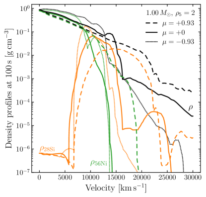
Figure 1: Profiles of the total mass density (black), ²⁸Si mass density (orange), and ⁵⁶Ni mass density (green) at $100\,\mathrm{s}$ for our $1.00\,M_{\sun}$, $\rho_{5}=2$ explosion model. Different line styles correspond to rays with different values of $\mu=+0.93$ (dashed), $0$ (solid), and $-0.93$ (dotted).

Each model explosion is initiated in FLASH via a hotspot along the symmetry axis in the helium shell. We designate the hemisphere containing the hotspot as the northern hemisphere. The ensuing helium detonation propagates around the surface of the WD towards the south pole, shedding a shock wave that travels into the core and eventually triggers a carbon core detonation near the symmetry axis in the southern hemisphere. This second detonation propagates back out and burns the majority of the core.

Figure 1 shows the resulting profiles of the total mass density, the ²⁸Si mass density, and the ⁵⁶Ni mass density for our $1.0\,M_{\sun}$ model with an initial helium shell base density, normalized to $10^{5}\,\mathrm{g\,cm^{-3}}$, of $\rho_{5}=\rho_{\rm base}/{\rm 10^{5}\,g\,cm^{-3}}=2$. Profiles are shown for three different values of $\mu=\cos\theta$, measured with respect to the symmetry axis in the northern hemisphere ($\mu=+1$ along the northern axis). It is evident that there is significant asymmetry imparted by the multi-dimensional nature of the helium detonation and the off-center carbon core detonation. In particular, as the carbon detonation propagates northwards from its birthplace in the southern hemisphere, it strengthens after it passes the center due to the negative density gradient and to the reduced effects of curvature. As a result, ²⁸Si is produced out to substantially higher velocities in the northern hemisphere, which will have a significant effect on the velocities inferred from spectra, which we discuss in Section 3.2. We refer the reader to Boos et al. (2021) for further details on the explosion models used in this work.

The post-processed abundances, densities, and temperatures from the FLASH simulations are interpolated onto two-dimensional axisymmetric velocity grids with $500\,\mathrm{km\,s^{-1}}$ resolution, which are then used as inputs for two-dimensional time-dependent radiation transport simulations with Sedona (Kasen et al., 2006). Sedona is a Monte-Carlo-based radiative transfer code that has been used extensively to study a variety of astrophysical transients (Kasen & Woosley, 2009; Kasen et al., 2009, 2011; Shen et al., 2010; Woosley & Kasen, 2011; Barnes & Kasen, 2013; Roth et al., 2016). The linelist is the same as that used in Shen et al. (2021) and contains up to the first 1000 lowest energy levels for all ionization states of interest. We treat line opacities in the “expansion opacity” formalism (Karp et al., 1977; Eastman & Pinto, 1993). We assume the absorption probability, $\epsilon$, is equal to a constant value of $1.0$ for all lines, which sets the line source functions equal to the Planck function. This implies that all radiative excitations end up contributing to the thermal pool of photons. We also assume that the ionization fractions and level populations are given by their local thermodynamic equilibrium (LTE) values. The frequency grid is spaced evenly in logarithmic space, with a constant multiplicative factor of 1.0003 between gridpoints. See Shen et al. (2021) for further details of the effects of these choices on one-dimensional WD detonation models.

3 Results

In this section, we present the light curves and spectra of our two-dimensional radiative transfer calculations and compare them to observations. Correlations among various quantities near maximum light are discussed in Section 4. Light curves and spectra are calculated along 15 viewing angles spaced evenly in $\mu=\cos\theta$, where $\theta$ is measured with respect to the symmetry axis. The helium shell detonation is ignited in the northern hemisphere, where $\mu>0$, and $\mu<0$ in the southern hemisphere, where the carbon core detonation is born. In this work, we present comparisons to observables from 10 days before to 3 days after $B$-band maximum, due to computational constraints and our LTE assumption, which becomes less accurate at later times. We will focus on modeling outside of this time frame in future studies.

3.1 Light curves

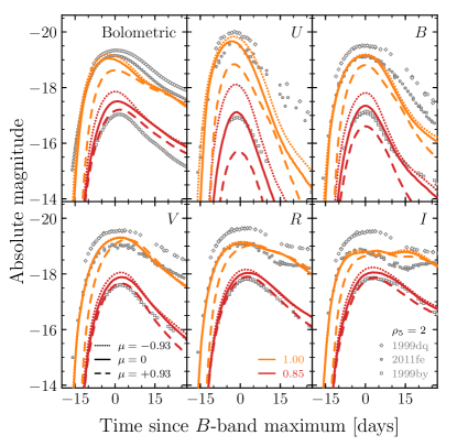
Figure 2: Multi-band light curves of our $0.85$ and $1.00\,M_{\sun}$ models with thin helium shells ($\rho_{5}=2$). Three lines of sight ($\mu=-0.93$, $0$, and $+0.93$) are shown for each model, corresponding to different linestyles. Gray points are observed SNe, as labeled; note that the observed “bolometric” light curves are more precisely quasi-bolometric light curves and are thus an underestimate of the true bolometric luminosities.

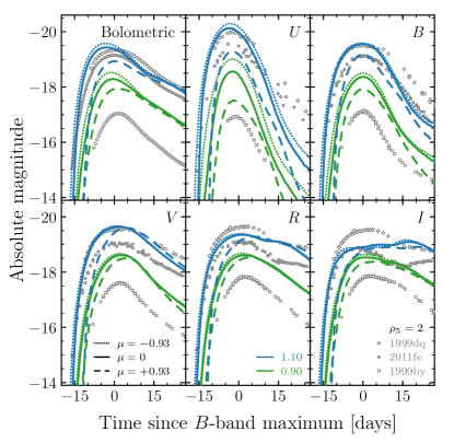
Figure 3: Same as Figure 2, but for models with masses of $0.9$ and $1.1\,M_{\sun}$.

Figures 2 and 3 show multi-band light curves for models with total masses of $0.85$, $0.90$, $1.00$, and $1.10\,M_{\sun}$ with the same initial helium shell base density of $\rho_{5}=2$. Different linestyles correspond to different viewing angles of $\mu=-0.93$, $0.0$, and $+0.93$, i.e., in the southern hemisphere, along the equator, and in the northern hemisphere, respectively. We do not show the light curves of the $1.02\,M_{\sun}$, $\rho_{5}=2$ models for clarity. They are similar to the light curves of the $1.00\,M_{\sun}$ model, but are slightly more luminous (the $B$-band maxima from different lines of sight are at most $0.1\,\mathrm{mag}$ brighter) as befits their somewhat higher ⁵⁶Ni production ($0.53\,M_{\sun}$ vs. $0.50\,M_{\sun}$).

Gray symbols in both figures represent photometry of subluminous SN 1999by (Garnavich et al., 2004; Stritzinger, 2005; Ganeshalingam et al., 2010), normal SN 2011fe (Munari et al., 2013; Pereira et al., 2013; Tsvetkov et al., 2013), and overluminous SN 1999dq (Stritzinger, 2005; Jha et al., 2006; Ganeshalingam et al., 2010). SN 1999dq’s light curve has been corrected for Milky Way reddening (Schlafly & Finkbeiner, 2011). Note that the observed “bolometric” light curves shown here and throughout this work are actually quasi-bolometric light curves, which neglect the flux bluer than the $U$-band and redder than the $I$-band. For the normal SN 2011fe and overluminous SN 1999dq, the quasi-bolometric and true bolometric luminosities are not significantly different (Suntzeff, 1996). However, for the subluminous SN 1999by, this may be as much as a 50% underestimate of the luminosity at later times, as we discuss below. We do not attempt to produce quasi-bolometric light curves from our models for comparison because they are significantly affected by our LTE approximation.

We note that non-LTE effects also have a significant impact on light curves after maximum light (Shen et al., 2021), especially in the $U$-, $B$-, and $I$-bands. We show the evolution of the light curves well past maximum for completeness, but we limit our post-maximum quantitative analysis to the (true) bolometric light curves, which should be relatively immune from non-LTE corrections.

The equatorial light curves for the $0.85$, $1.0$, and $1.1\,M_{\sun}$ models provide a reasonable fit in all bands to the three sets of observed SN photometry up to maximum light, with models of increasing mass matching observations of increasingly luminous SNe. The largest discrepancy is in the $I$-band comparison of the $1.1\,M_{\sun}$ model and SN 1999dq. We note that a similar difference is seen in the one-dimensional non-LTE models of Shen et al. (2021).

The light curves along varying lines of sight are markedly different, particularly in the bluer bands, and especially for the lowest mass model, for which the maximum $B$-band magnitudes vary by $>1\,\mathrm{mag}$. The variation in maximum magnitudes is not as significant for the higher mass models, but it is large enough that the brightest $1.0\,M_{\sun}$ model line of sight reaches the same magnitude as the dimmest $1.1\,M_{\sun}$ model line of sight. There is a similar disparity in the timescales to reach maximum light at different viewing angles. The most rapidly rising viewing angles for the $1.0$ and $1.1\,M_{\sun}$ models reach maximum light in nearly the same time that the most slowly rising $0.85\,M_{\sun}$ model line of sight does.

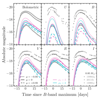
Figure 4: Same as Figure 2, but for $0.85\,M_{\sun}$ models with $\rho_{5}=2$ and $3$.

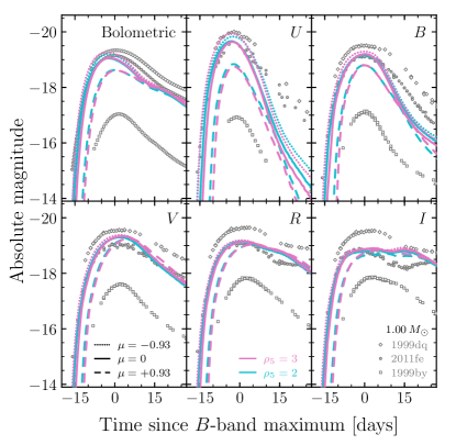
Figure 5: Same as Figure 4, but for $1.00\,M_{\sun}$ models.

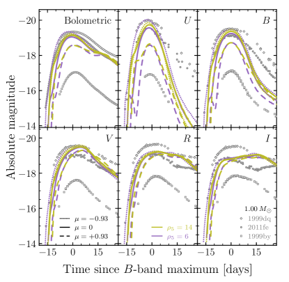
Figure 6: Same as Figure 5, but for base densities of $\rho_{5}=6$ and $14$.

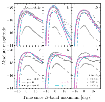
Figure 7: Same as Figure 4, but for $1.10\,M_{\sun}$ models.

We compare models with the same total masses but different helium shell base densities in Figures 4 – 7. For the $1.0$ and $1.1\,M_{\sun}$ models with $\rho_{5}=2$ and $3$ (Figures 5 and 7), the differences among the light curves are relatively minimal. Peak magnitudes and light curve shapes are nearly identical for all viewing angles. However, the differences are more significant for the $0.85\,M_{\sun}$ models shown in Figure 4: the $\rho_{5}=2$ model is brighter in $B$-band than the $\rho_{5}=3$ model when viewed from the northern hemisphere, where the helium shell detonation is ignited, possibly due to the much larger amount of Ti and associated line-blanketing in the northern shell of the thicker helium shell model, but is dimmer when viewed from the southern hemisphere, likely due to the larger amount of ⁵⁶Ni produced by the $\rho_{5}=3$ model.

There are also significant differences for the thick helium shell $1.0\,M_{\sun}$ models shown in Figure 6. While the amount of radioactive ⁴⁸Cr and ⁵⁶Ni produced in the helium shell is very low for the $1.0\,M_{\sun}$, $\rho_{5}=2$ and $3$ models ($<2\times 10^{-5}\,M_{\sun}$ for both), the $\rho_{5}=6$ and $14$ models produce significantly more radioactive material: $7\times 10^{-3}$ and $0.05\,M_{\sun}$, respectively. The radioactive decay of this material near the surface of the ejecta leads to early “shoulders” and “humps” in the light curves of these models. Similar features are seen in previous studies of one-dimensional relatively massive helium shell models (Woosley & Weaver, 1994; Polin et al., 2019), which have been invoked to explain several peculiar SNe Ia (De et al., 2019; Jacobson-Galán et al., 2020). The present paper focuses on thin-shell models, but we include results from these two thick-shell models for completeness; we leave a more thorough examination of models with massive helium shells to future work.

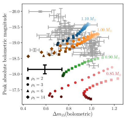
Figure 8: Peak absolute bolometric magnitude vs. $\Delta m_{15}({\rm bolometric})$, i.e., the bolometric version of the Phillips (1993) relation. Gray error bars are observational data from Scalzo et al. (2019), and results from our theoretical models are as labeled. Light to dark colors are different lines of sight with increasing values of $\mu$ from $-0.93$ to $+0.93$, equally spaced in $\mu$. The black error bar shows the maximum differences between the LTE and non-LTE results from Shen et al. (2021) for the relevant quantities.

Figure 8 shows the bolometric version of the Phillips (1993) relationship, comparing the maximum bolometric magnitude to the 15-day decline in bolometric magnitude following the time of maximum, $\Delta m_{15}({\rm bolometric})$. (Given the differences between LTE and non-LTE results presented in Shen et al. 2021, we do not present analogous comparisons in any broad-band filters.) Theoretical models are as labeled, with lines of sight from southern to northern hemispheres corresponding to symbols of increasing darkness. Observed values from Scalzo et al. (2019) are in gray. The black error bar shows the differences in bolometric peak magnitude and in $\Delta m_{15}({\rm bolometric})$ between LTE and non-LTE radiative transfer calculations of one-dimensional sub-Chandraskehar-mass WD detonations from Shen et al. (2021). These differences should not be thought of as directly applicable to the models we discuss in this paper, since the one-dimensional bare WD simulations analyzed in Shen et al. (2021) are obviously different from multi-dimensional thin-shell double detonation models, but they may be suggestive of the possible changes when non-LTE multi-dimensional radiation transport is performed in the future.

Most of the lines of sight for the $1.0$ and $1.1\,M_{\sun}$ models yield results within the observed range. However, the northernmost lines of sight for the $1.0\,M_{\sun}$ models with higher helium shell base densities ($\rho_{5}\geq 3$) lead to light curves that fade too slowly for their peak luminosity. There are two SNe Ia with similar parameters, but they are the peculiar SN 2006bt and SN 2006ot (Foley et al., 2010; Stritzinger et al., 2011). Even given the possible variance between LTE and non-LTE models suggested by the black error bar, double detonations with $\rho_{5}\gtrsim 6$ helium shells appear to be ruled out as the dominant progenitors of SNe Ia.

The Scalzo et al. (2019) observed sample contains very few SNe Ia with bolometric luminosities as low as those produced by our $0.9\,M_{\sun}$ model due to the magnitude-limited nature of the surveys from which they draw. The few observed low-luminosity SNe that do exist in the sample are consistent with the bolometric decline rates of the southern viewing angles. However, similar to the $1.0$ and $1.1\,M_{\sun}$ thick shell models, the $0.9\,M_{\sun}$ model’s northernmost lines of sight do not appear to match SNe found in nature, with the repeated caveat that the observed sample size is small.

None of the observed light curves in the sample probes the faintest end of the SN Ia luminosity distribution, with similar bolometric magnitudes to those of the low-mass $0.85\,M_{\sun}$ models. We have examined some of the SN 1991bg-like SNe in the literature but did not find any truly bolometric results. Several studies do report quasi-bolometric results (e.g., Stritzinger 2005 and Taubenberger et al. 2008), integrating the flux in the $U$-, $B$-, $V$-, $R$-, and $I$-bands; however, the quasi-bolometric to bolometric flux ratios of our low-mass models evolve significantly with time and become as low as 50% 15 days after the time of bolometric maximum. Furthermore, while the true bolometric light curve is relatively immune from non-LTE corrections, the quasi-bolometric light curve is much more sensitive to non-LTE effects, due to the redistribution of flux into the Ca ii near-infrared triplet feature at wavelengths where the transmission of the $I$-band begins to decrease. Thus, we do not attempt to match our low-mass models to the quasi-bolometric data in the literature.

3.2 Spectra

In Figures 9 – 15, we show near-maximum-light spectra of a subset of our models from different viewing angles, scaled so that the difference between the maximum and minimum of each spectrum is equal to 1. We also show spectra of observed SNe at the same phase with respect to the time of $B$-band maximum, chosen to approximately match the light curve evolution viewed along the equatorial line of sight of each model. The observed spectra are scaled by an arbitrary factor that is constant within each figure but differs between figures.

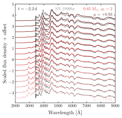
Figure 9: Spectra of the $0.85\,M_{\sun}$, $\rho_{5}=2$ model from different lines of sight at $-2.2$ days from the time of $B$-band maximum. Values of $\mu$ decrease from top to bottom. Gray lines are the spectrum of SN 1999by at $-2.2$ days, scaled by an arbitrary constant and reproduced 15 times for ease of comparison.

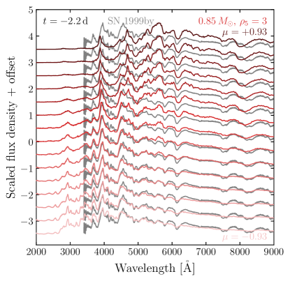
Figure 10: Same as Figure 9, but for the model with $\rho_{5}=3$.

As Figure 9 shows, the subluminous SN 1999by (Matheson et al., 2008) provides a particularly good fit to the equatorial spectrum of the $0.85\,M_{\sun}$, $\rho_{5}=2$ model and satisfactorily matches the spectra further into the southern hemisphere (the hemisphere where the carbon core detonation is ignited). However, in the northern hemisphere, the Ti ii trough located near $4000\,\mathrm{\AA}$ becomes very deep, due to the lower temperatures caused by both the more radially extended distribution of Ti and the lower flux along these lines of sight. Furthermore, the observed wavelength of the Si ii $\lambda 6355$ absorption minimum is slightly blueshifted with respect to the models; we discuss this further in Section 4. The overall fits to the $0.85\,M_{\sun}$, $\rho_{5}=3$ model lines of sight shown in Figure 10 are not as good as those for the $\rho_{5}=2$ model, matching expectations from the larger color deviations seen in Figure 4, and a similar mismatch of the Ti ii trough is seen in the northern hemisphere of this model as well.

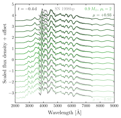
Figure 11: Same as Figure 9, but for the $0.90\,M_{\sun}$, $\rho_{5}=2$ model $-0.4$ days from the time of $B$-band maximum. Gray lines are the spectrum of SN 1998bp at the same time.

Our $0.9\,M_{\sun}$ model is compared to the transitional SN 1998bp (Matheson et al., 2008), corrected for Milky Way reddening (Schlafly & Finkbeiner, 2011), in Figure 11. The fits to the lines of sight near the equator are particularly good. In the southern hemisphere (fainter lines), the model absorption features throughout the optical are not quite as deep as for the observed spectrum; in the northern hemisphere (darker lines), the model absorption complex near $4000\,\mathrm{\AA}$, containing Mg ii, Si ii, Fe ii, and possibly Ti ii lines, is too deep.

For this and the higher-mass $1.0$ and $1.1\,M_{\sun}$ models, there is a strong Si ii velocity dependence on the viewing angle: velocities in the southern hemisphere are roughly similar to each other, and they increase as the viewing angle moves northwards. This trend matches the qualitative features seen in Figure 1, in which the southern and equatorial ²⁸Si density profiles are relatively similar, while the northern density profile extends to higher velocities. A similar distribution of velocities with respect to viewing angle was found in Townsley et al. (2019)’s radiative transfer calculations and was used by Zhang et al. (2020) to provide a broad match to the observed SN Ia velocity distribution.

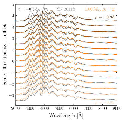
Figure 12: Same as Figure 9, but for the $1.00\,M_{\sun}$, $\rho_{5}=2$ model $-0.8$ days from the time of $B$-band maximum. Gray lines are the spectrum of SN 2011fe at the same time.

Normal SN 2011fe (Mazzali et al., 2014) is compared to the lowest and highest helium shell base density $1.0\,M_{\sun}$ models in Figures 12 and 13. As before, the equatorial line of sight for the lowest helium shell density model yields a reasonable fit to the observed spectrum, although there are some discrepancies (e.g., the depth of the Si ii $\lambda 4130$ feature and the locations of the Si ii $\lambda 4130$ and $\lambda 6355$ absorption minima). There is similar agreement throughout the southern hemisphere. However, the spectra viewed from the north deviate significantly from that of SN 2011fe, particularly when comparing the velocities of the features: the model velocities are blueshifted by up to $4000\,\mathrm{km\,s^{-1}}$ for the northernmost line of sight.

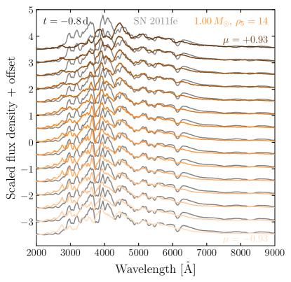
Figure 13: Same as Figure 12, but for the model with $\rho_{5}=14$.

Figure 13 compares SN 2011fe’s near-maximum-light spectrum to those of the $1.0\,M_{\sun}$, thickest helium shell ($\rho_{5}=14$) model. While there is some agreement at the equator and in the southern hemisphere, there are larger discrepancies than for the thin shell ($\rho_{5}=2$) model. In the northern hemisphere, the velocity disagreements are not as striking as for the thin shell case, but the model spectra have much more absorption below $4000\,\mathrm{\AA}$, commensurate with the mismatch in $U-B$ colors seen in Figure 6.

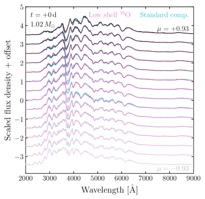
Figure 14: Same as Figure 9, but for the $1.02\,M_{\sun}$, $\rho_{5}=2$ models $+0.0$ days from the time of $B$-band maximum. Cyan lines show spectra of the model with a standard initial helium shell composition; magenta lines show spectra for the model with a reduced ¹⁶O initial shell abundance.

We examine the effects of changing the initial ¹⁶O shell abundance in Figure 14. Cyan lines show spectra for a $1.02\,M_{\sun}$, $\rho_{5}=2$ model with an initial helium shell composition identical to that of the models with different masses. Magenta lines show spectra for a $1.02\,M_{\sun}$ model with a reduced ¹⁶O mass fraction in the shell of $0.015$. The spectra are nearly identical from all viewing angles, except for a slight deviation in the Ca ii H&K feature near the equator: the model with a reduced ¹⁶O shell abundance does not have as strong an absorption feature as the standard abundance model, due in part to a two-fold reduction in the amount of Ca that is synthesized in the shell.

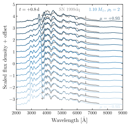
Figure 15: Same as Figure 9, but for the $1.10\,M_{\sun}$, $\rho_{5}=2$ model $+0.8$ days from the time of $B$-band maximum. Gray lines are the spectrum of SN 1999dq at the same time.

In Figure 15, we compare the near-maximum-light spectra of our $1.1\,M_{\sun}$, $\rho_{5}=2$ model to that of the overluminous SN 1999dq (Matheson et al., 2008), which is corrected for Milky Way reddening (Schlafly & Finkbeiner, 2011). The equatorial line of sight is somewhat less of a satisfactory fit than for the previous comparisons, but the model still captures the basic features of the observed spectrum. However, there is a significant discrepancy in the Si ii $\lambda 6355$ velocity, which is even more striking in the northern hemisphere; the observed spectrum’s Si ii $\lambda 6355$ feature is redshifted by $8000\,\mathrm{km\,s^{-1}}$ compared to that of the southernmost line of sight. The velocity agreement is better for the lines of sight in the southern hemisphere, but the depths of the Si ii $\lambda 5972$ and $\lambda 6355$ features do not match well.

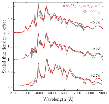
Figure 16: Spectra of the $0.85\,M_{\sun}$, $\rho_{5}=2$ model viewed from the equator at the labeled times with respect to the time of $B$-band maximum. Gray lines are spectra of SN 1999by at the same times, each of which is scaled by eye to provide a best fit to the theoretical spectrum.

Figures 16 – 19 show the spectral time evolution of each thin shell ($\rho_{5}=2$) model as viewed along the line of sight labeled in each figure. Gray lines are observed spectra at the labeled times, each of which is arbitrarily scaled to provide a best fit by eye to the theoretical model. The $0.85\,M_{\sun}$ model is compared to SN 1999by (Garnavich et al., 2004; Matheson et al., 2008) in Figure 16. Some aspects are well-reproduced (e.g., the Ti ii trough deepens with time in a similar way for both the model and observed spectra), but some details do not match precisely, possibly as a consequence of our LTE, expansion opacity approximation (Kasen et al., 2006; Shen et al., 2021): e.g., as discussed previously, the wavelength of the Si ii $\lambda 6355$ absorption minimum is slightly discrepant, and the depths of some lines are not an exact match. However, the overall correspondence is encouraging.

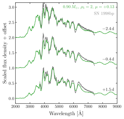
Figure 17: Same as Figure 16, but for the $0.90\,M_{\sun}$, $\rho_{5}=2$ model compared to SN 1998bp.

The time evolution of our $0.9\,M_{\sun}$ model is shown in Figure 17, compared to that of SN 1998bp (Matheson et al., 2008), which has been corrected for Milky Way reddening (Schlafly & Finkbeiner, 2011). The spectra do not cover as large a time window as in the other figures, but within the observed range, the model spectra evolve similarly to the observed spectra. For example, the feature near $4300\,\mathrm{\AA}$ deepens and flattens with time for both the model and the observed spectra. There are some slight discrepancies in the depths of some other absorption features, but there is good agreement overall.

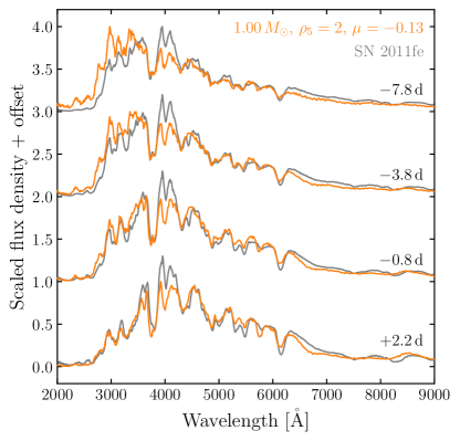
Figure 18: Same as Figure 16, but for the $1.00\,M_{\sun}$, $\rho_{5}=2$ model compared to SN 2011fe.

Figure 18 compares the evolution of the $1.00\,M_{\sun}$ model to SN 2011fe (Mazzali et al., 2014). Again, the theoretical model provides an adequate match to the observed spectrum in many respects. However, as noted in the discussion of the maximum-light spectra (Figure 12), the model spectra do not have as much absorption in the Si ii $\lambda 4130$ feature, and the absorption minima of the Si ii $\lambda 4130$ and $\lambda 6355$ lines are somewhat blueshifted with respect to the observed spectra.

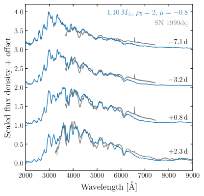
Figure 19: Same as Figure 16, but for the $1.10\,M_{\sun}$, $\rho_{5}=2$ model compared to SN 1999dq.

Our $1.10\,M_{\sun}$ model is compared to SN 1999dq (Matheson et al., 2008; Silverman et al., 2012), corrected for Milky Way reddening (Schlafly & Finkbeiner, 2011), in Figure 19. Unlike the previous three figures, for which lines of sight near the equator were used, this figures shows the evolution of a line of sight near the southern pole, for which the Si ii $\lambda 6355$ velocity provides a better match to the observed velocity. As with the previous comparisons, the match between the model and observed spectra is not exact, with discrepancies in the depths of several absorption features. However, most of the absorption features across the optical range deepen with time in a similar way, and, in general, the agreement is satisfactory.

4 Maximum light correlations

In this section, we perform an exploration of photometric and spectroscopic correlations in our model observables near maximum light. We caution that, due to the LTE nature of our radiation transport calculations, there are almost certainly systematic offsets in the derived quantities, and so these results should be viewed as merely suggestive.

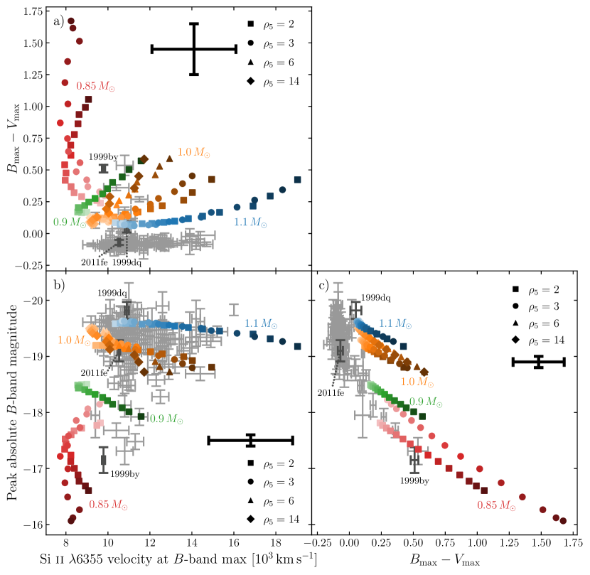
Figure 20: Correlations between a) $B_{\rm max}-V_{\rm max}$ and Si ii $\lambda 6355$ velocity; b) $B_{\rm max}$ and Si ii velocity; and c) $B_{\rm max}$ and $B_{\rm max}-V_{\rm max}$. Colored points are our theoretical models, as labeled, with $\mu$ increasing with darkness. Black error bars represent the maximum differences in the relevant quantities between LTE and non-LTE results from Shen et al. (2021). The velocity error bar includes an additional $1000\,\mathrm{km\,s^{-1}}$ of variance from the D⁶ slingshot effect. Gray error bars are observed SNe from Burrow et al. (2020); dark gray error bars are individual SNe.

Figure 20 compares three near-maximum light quantities: the peak absolute $B$-band magnitude ($B_{\rm max}$), the Si ii $\lambda 6355$ velocity at the time of $B$-band maximum, as measured by the blueshift of the absorption minimum, and the color defined by the difference between $B_{\rm max}$ and the absolute $V$-band maximum magnitude, $V_{\rm max}$, which occurs several days after the time of $B$-band maximum. Each panel shows a different comparison of two of the three quantities: color vs. Si velocity in panel a, $B_{\rm max}$ vs. Si velocity in panel b, and $B_{\rm max}$ vs. color in panel c. In each panel, colored symbols represent results from our simulations as labeled, with $\mu$ of the viewing angle increasing with darkness.

Many similar comparisons have been made in observational data (e.g., Hachinger et al. 2006; Foley & Kasen 2011; Foley et al. 2011; Blondin et al. 2012; Maguire et al. 2014; Zheng et al. 2018). Here, we use the recent compilation from Burrow et al. (2020), which is shown as gray error bars in each panel. Dark gray error bars represent SN 1999by (Garnavich et al., 2004; Hachinger et al., 2006), SN 2011fe (Pereira et al., 2013; Silverman et al., 2015; Zhang et al., 2016), and SN 1999dq (Stritzinger et al., 2006; Ganeshalingam et al., 2010; Zheng et al., 2018). Note that Burrow et al. (2020)’s compilation includes SNe from Zheng et al. (2018), who did not include color information, so some SNe in panel b are not represented in the other two panels.

The black error bar in each panel shows the maximal differences in the relevant quantities between the LTE and non-LTE results for the one-dimensional bare WD core detonations in Shen et al. (2021), as an estimate of the possible offset between the LTE results in this paper and future non-LTE calculations. We also add an additional $1000\,\mathrm{km\,s^{-1}}$ of variance to the representative velocity error bars to account for the slingshot effect: if SNe Ia arise from the “dynamically driven double-degenerate double-detonation” (D⁶) scenario, and if the companion WD survives (Shen et al., 2018b), the SN ejecta will be born with a $\sim 1000\,\mathrm{km\,s^{-1}}$ randomly oriented kick.

We emphasize that the black error bars do not represent random, Gaussian errors in the theoretical results. Furthermore, there are likely systematic shifts in the relevant quantities between LTE and non-LTE results. For example, the colors of the non-LTE simulations in Shen et al. (2021) are consistently bluer than the LTE colors for WD masses $\geq 0.9\,M_{\sun}$, but redder for the lowest-mass $0.85\,M_{\sun}$ models. For the highest Si ii $\lambda 6355$ velocities, found in the $1.1\,M_{\sun}$ explosion model, the non-LTE CMFGEN results are $1200\,\mathrm{km\,s^{-1}}$ slower than the LTE Sedona results, while for the $0.85\,M_{\sun}$ model, the CMFGEN results are $300\,\mathrm{km\,s^{-1}}$ faster than the LTE Sedona results.

The $1.0$ and $1.1\,M_{\sun}$ models satisfactorily cover the range of observed peak $B$-band magnitudes and Si ii velocities for normal and overluminous SNe Ia. However, the $1.1\,M_{\sun}$ models viewed from the northernmost lines of sight extend to higher velocities than observed in the Burrow et al. (2020) sample, reaching up to $19000\,\mathrm{km\,s^{-1}}$. The lack of observed SNe with such high velocities may be due to the relative rarity of $1.1\,M_{\sun}$ explosions combined with the low probability of viewing such an explosion from the northernmost lines of sight. Moreover, future non-LTE calculations may result in a systematic redshift of these highest velocities, as found by Shen et al. (2021). On the other end of the mass range, the $0.85\,M_{\sun}$ models yield Si ii velocities that are $1000-2000\,\mathrm{km\,s^{-1}}$ slower than observed in subluminous SNe Ia. The $0.85\,M_{\sun}$ models’ northernmost lines of sight also reach fainter peak $B$-band magnitudes than observed, by up to $1\,\mathrm{mag}$.

The largest discrepancy between our models and observed data is in the $B_{\rm max}-V_{\rm max}$ colors: the theoretical models are generally redder than observed SNe Ia. Focusing on the thin-shell $\rho_{5}=2$ and $\rho_{5}=3$ cases, the $1.0$ and $1.1\,M_{\sun}$ models are up to $0.5\,\mathrm{mag}$ redder than observed SNe Ia with the same peak $B$-band magnitudes or Si ii $\lambda 6355$ velocities. However, given the systematic blueward shift from LTE to non-LTE colors found by Shen et al. (2021) for detonations of WDs with similar masses, this color discrepancy may disappear with more physical radiative transfer calculations.

Meanwhile, the $0.85\,M_{\sun}$ models extend to much redder colors than observed, by as much as $1.1\,\mathrm{mag}$ for the $\rho_{5}=3$ model’s northernmost line of sight. These discrepancies in color and peak $B$-band magnitude are far beyond the differences between Shen et al. (2021)’s LTE and non-LTE results and constitute evidence that $0.85\,M_{\sun}$ WDs do not explode as subluminous SNe Ia. There is a lower limit to the mass of a WD that can undergo a converging shock double detonation, because the critical ingoing shock strength necessary to trigger a core detonation increases with decreasing central density (Shen & Bildsten, 2014); a $0.85\,M_{\sun}$ WD may be below this mass limit.

It is also possible that $0.85\,M_{\sun}$ WDs do explode but belong to other observed classes of transients. Type Iax supernovae (Foley et al., 2013; Jha, 2017) are one such class of candidates, but they possess even lower Si ii $\lambda 6355$ velocities at $B$-band maximum, $<7000\,\mathrm{km\,s^{-1}}$, than seen in our models. Ca-strong transients (Perets et al., 2010; Kasliwal et al., 2012; Shen et al., 2019) are even fainter than the dimmest lines of sight of our $0.85\,M_{\sun}$ models, with peak $B$-band magnitudes $>-15$.

Another potential observational counterpart are the SN 2002es-like SNe, including SN 2006bt, PTF 10ops, and iPTF 14atg (Foley et al., 2010; Maguire et al., 2011; Ganeshalingam et al., 2012; Cao et al., 2015; White et al., 2015; Taubenberger, 2017). These SNe form a fairly heterogeneous class, with Si ii $\lambda 6355$ velocities at $B$-band maximum that range from $6000$ to $10000\,\mathrm{km\,s^{-1}}$ and $B_{\rm max}$ ranging from $-17.6$ to $-19$. Unlike Type Iax supernovae, which strongly prefer young stellar populations, SN 2002es-like SNe explode preferentially in early-type galaxies, matching binary population synthesis predictions of the host galaxies of double WD mergers with primary masses $\sim 0.85\,M_{\sun}$ (Shen et al., 2017). However, while iPTF 14atg’s maximum light spectrum does provide a reasonable match to the $0.85\,M_{\sun}$, $\rho_{5}=2$ model viewed from the equatorial line of sight, the large range of velocities observed for SN 2002es-likes and the lack of dimmer and very red SN 2002es-like SNe appears to rule out a correspondence between these models and this class as a whole.

In addition to the three maximum light observables we focus on in Figure 20, other spectral indicators have also been studied previously, including the time derivative of the Si ii $\lambda 6355$ velocity, (pseudo-)equivalent widths and depths of various lines, and the velocity of nebular phase iron-group emission lines (e.g., Nugent et al. 1995; Benetti et al. 2005; Branch et al. 2006; Taubenberger et al. 2008; Maeda et al. 2010b, a; Foley et al. 2011; Blondin et al. 2011, 2012; Livneh & Katz 2020). We choose to focus on $B_{\rm max}$, the Si ii $\lambda 6355$ velocity, and $B_{\rm max}-V_{\rm max}$ because these three indicators are more robust to the effects of Monte Carlo noise and change less between LTE and non-LTE calculations than other features. In particular, nebular phase spectra clearly necessitate non-LTE simulations, and the interpretation of these spectra is made even more difficult due to line blending and time variability of the inferred velocities (Black et al., 2016; Botyánszki & Kasen, 2017; Graham et al., 2017). A more detailed examination of correlations among these and other model observables awaits future high-resolution, non-LTE radiative transfer calculations.

5 Comparison to previous work

Radiative transfer simulations of sub-Chandrasekhar-mass WD detonations have been carried out previously, but the majority of these have assumed spherical symmetry (Woosley et al., 1986; Woosley & Weaver, 1994; Sim et al., 2010; Woosley & Kasen, 2011; Blondin et al., 2017; Shen et al., 2018a, 2021; Goldstein & Kasen, 2018; Polin et al., 2019; Wygoda et al., 2019a, b; Kushnir et al., 2020). While qualitative progress can be made in one dimension (see, e.g., the agreement with the Phillips 1993 relationship in the non-LTE, large nuclear reaction network study by Shen et al. 2021), more detailed comparisons require multiple dimensions, due to the inherent asymmetry imparted by the laterally propagating helium shell detonation.

Another subset of radiation transport calculations have focused on explosions following double WD mergers in which the companion WD is completely disrupted (Pakmor et al., 2010, 2011, 2012, 2021; Moll et al., 2014; Raskin et al., 2014; van Rossum et al., 2016). These are qualitatively different from the simulations in this work, which assume that only one WD explodes, leaving the companion star, be it a WD or a non-degenerate star, mostly intact. We thus do not attempt detailed comparisons to these studies.

The first multi-dimensional radiative transfer simulations of single sub-Chandrasekhar-mass WD detonations were performed by Kromer et al. (2010), with angle-averaged results reported in Fink et al. (2010). Due to possible issues with the implementation of detonation physics, the nucleosynthesis in the models used in these studies differs significantly from more recent work, making a direct comparison between our predicted observables difficult. However, there is qualitative agreement between our study and that of Kromer et al. (2010). Both sets of calculations find a strong dependence on viewing angle, with maximum light colors becoming bluer as the line of sight moves from the north pole, where the helium shell detonation is ignited, to the south pole. Most models in both studies are also redder at maximum light than observed SNe with similar luminosities, although it is difficult to disentangle the effects of the radiative transfer approximations in both studies from the thicker helium shells present in the previous work. The closest match in initial conditions for a quantitative comparison is between their model 2, initially consisting of a $0.92\,M_{\sun}$ core and a $0.084\,M_{\sun}$ helium-rich envelope, and our thickest shell $1.0\,M_{\sun}$, $\rho_{5}=14$ model, which has a $0.90\,M_{\sun}$ core and a $0.10\,M_{\sun}$ helium-rich envelope. Our model produces significantly more ⁵⁶Ni ($0.56\,M_{\sun}$) than theirs ($0.34\,M_{\sun}$) and commensurately less intermediate-mass element material than in their model. It is thus not surprising that Kromer et al. (2010) find peak $B$-band magnitudes ranging from $-16.1$ to $-18.3$ depending on the line of sight, whereas we derive peak magnitudes of $-18.7$ to $-19.5$. We note that Sim et al. (2012) also perform a similar study, but with even lower-mass WDs (total masses $\leq 0.79\,M_{\sun}$) and very thick helium shells of $0.21\,M_{\sun}$ for which we do not have comparable models.

Using very similar methodology to Boos et al. (2021), Townsley et al. (2019) simulated the two-dimensional detonation of a $1.0+0.02\,M_{\sun}$ WD and approximated multi-dimensional radiative transfer by constructing one-dimensional spherical profiles from wedges of the two-dimensional explosion simulation. The choice was made to renormalize the density profiles of these wedges to yield one-dimensional spheres with total masses equal to $1.0\,M_{\sun}$, which is likely the reason for the different light curve shapes compared to the results in this work; in particular, the multi-band light curves viewed from the northern hemisphere evolve more rapidly in Townsley et al. (2019)’s work. However, the near-maximum-light spectra are similar, with Si ii $\lambda 6355$ velocities in the southern hemisphere that match those of the present work and of SN 2011fe, while those in the northern hemisphere are similarly too fast by several thousand ${\rm km\,s^{-1}}$.

Gronow et al. (2020) performed several three-dimensional double detonation simulations. The best comparisons between their models and ours are their M1a and M2a models and our $1.0\,M_{\sun}$, $\rho_{5}=6$ model. Their radiative transfer results are much redder than ours, with angle-averaged values of $B_{\rm max}-V_{\rm max}=0.9$ and $1.1$, while our angle-averaged results yield $B_{\rm max}-V_{\rm max}=0.2$. However, the two sets of models do not differ drastically in terms of nucleosynthesis: total ⁵⁶Ni yields differ by $<10\%$, with similar differences for other important elements. Furthermore, while Gronow et al. (2020)’s M2a model is ignited via the “scissors” mechanism due to the enhanced carbon abundance in the helium shell, their M1a explodes in a similar way to our models, via a converging shock, so asymmetry is not the root cause of the discrepancies.

Gronow et al. (2021) update their previous results with a large suite of double detonation calculations. However, they only present bolometric light curves; future work will provide more detailed radiative transfer analysis. They find similar bolometric trends within each model: the hemisphere opposite the initial helium-shell detonation yields brighter lines of sight that fade more rapidly, at least in a bolometric sense. There are slight quantitative differences when the observables are examined at a more detailed level (e.g., while their M10_02 model provides a good match to our $1.0\,M_{\sun}$, $\rho_{5}=3$ model, their M08_03 model, which is close to our $0.85\,M_{\sun}$, $\rho_{5}=2$ model, is somewhat brighter and fades more slowly), but the overall correspondence is fairly satisfactory.

6 Conclusions

In this work, we have performed multi-dimensional radiation transport calculations of the suite of sub-Chandrasekhar-mass WD double detonation models described in Boos et al. (2021). We find broad agreement with the light curves and spectra of the entire range of non-peculiar SNe Ia, from subluminous to overluminous examples. Increasing the total mass of the exploding WD leads to brighter and bluer SNe and increases the velocities of absorption features in maximum-light spectra. Varying the viewing angle from the southern hemisphere (where the carbon core detonation begins) to the northern hemisphere (where the helium detonation is ignited) yields dimmer and redder SNe and increases spectral velocities for most models.

There are several significant discrepancies between our theoretical models and observed SNe. The Si ii velocities at maximum light of the $1.1\,M_{\sun}$ models viewed from the northernmost lines of sight are at the limit of, and possibly faster than, the fastest velocities observed for SNe Ia. Meanwhile, the velocities of the $0.85\,M_{\sun}$ models are slower than for any observed SNe Ia, and the fluxes viewed from the north are fainter than for even the dimmest SNe Ia. Moreover, the maximum-light colors of all of our models are generally several tenths of a magnitude redder than for observed SNe, and as much as $\sim 1\,\mathrm{mag}$ redder for the $0.85\,M_{\sun}$ model’s northern lines of sight. The magnitude of the discrepancies for the $0.85\,M_{\sun}$ models may indicate that the minimum mass for a successful core detonation lies between $0.85$ and $0.90\,M_{\sun}$.

Future calculations that include more accurate physics and initial conditions may alleviate the color and velocity discrepancies for the higher masses. The radiative transfer simulations in the present work assume LTE for the level and ionization state populations, but Shen et al. (2021) have found that non-LTE calculations yield corrections that will help to reduce the aforementioned differences. Furthermore, the existence of the companion WD is neglected in this study. If it is located in the northern hemisphere at the time of the explosion, the companion WD will alter the velocity and thermodynamic structure of the northernmost SN ejecta, possibly slowing it down and depositing enough energy to yield better color and velocity matches to observations.

References

- Barnes & Kasen (2013) Barnes, J., & Kasen, D. 2013, ApJ, 775, 18, doi: 10.1088/0004-637X/775/1/18
- Benetti et al. (2005) Benetti, S., Cappellaro, E., Mazzali, P. A., et al. 2005, ApJ, 623, 1011, doi: 10.1086/428608
- Bildsten et al. (2007) Bildsten, L., Shen, K. J., Weinberg, N. N., & Nelemans, G. 2007, ApJ, 662, L95, doi: 10.1086/519489
- Black et al. (2016) Black, C. S., Fesen, R. A., & Parrent, J. T. 2016, MNRAS, 462, 649, doi: 10.1093/mnras/stw1680
- Blondin et al. (2017) Blondin, S., Dessart, L., Hillier, D. J., & Khokhlov, A. M. 2017, MNRAS, 470, 157, doi: 10.1093/mnras/stw2492
- Blondin et al. (2011) Blondin, S., Kasen, D., Röpke, F. K., Kirshner, R. P., & Mandel, K. S. 2011, MNRAS, 417, 1280, doi: 10.1111/j.1365-2966.2011.19345.x
- Blondin et al. (2012) Blondin, S., Matheson, T., Kirshner, R. P., et al. 2012, AJ, 143, 126, doi: 10.1088/0004-6256/143/5/126
- Boos et al. (2021) Boos, S. J., Townsley, D. M., Shen, K. J., Caldwell, S., & Miles, B. J. 2021, ApJ, accepted (arXiv:2101.12330), arXiv:2101.12330. https://arxiv.org/abs/2101.12330
- Botyánszki & Kasen (2017) Botyánszki, J., & Kasen, D. 2017, ApJ, 845, 176, doi: 10.3847/1538-4357/aa81d8
- Branch et al. (2006) Branch, D., Dang, L. C., Hall, N., et al. 2006, PASP, 118, 560, doi: 10.1086/502778
- Burrow et al. (2020) Burrow, A., Baron, E., Ashall, C., et al. 2020, ApJ, 901, 154, doi: 10.3847/1538-4357/abafa2
- Cao et al. (2015) Cao, Y., Kulkarni, S. R., Howell, D. A., et al. 2015, Nature, 521, 328, doi: 10.1038/nature14440
- Colgate & McKee (1969) Colgate, S. A., & McKee, C. 1969, ApJ, 157, 623, doi: 10.1086/150102
- Dan et al. (2012) Dan, M., Rosswog, S., Guillochon, J., & Ramirez-Ruiz, E. 2012, MNRAS, 422, 2417, doi: 10.1111/j.1365-2966.2012.20794.x
- De et al. (2019) De, K., Kasliwal, M. M., Polin, A., et al. 2019, ApJ, 873, L18, doi: 10.3847/2041-8213/ab0aec
- Dubey et al. (2009) Dubey, A., Reid, L. B., Weide, K., et al. 2009, Parallel Computing, 35, 512
- Eastman & Pinto (1993) Eastman, R. G., & Pinto, P. A. 1993, ApJ, 412, 731, doi: 10.1086/172957
- Fink et al. (2007) Fink, M., Hillebrandt, W., & Röpke, F. K. 2007, A&A, 476, 1133, doi: 10.1051/0004-6361:20078438
- Fink et al. (2010) Fink, M., Röpke, F. K., Hillebrandt, W., et al. 2010, A&A, 514, A53, doi: 10.1051/0004-6361/200913892
- Foley & Kasen (2011) Foley, R. J., & Kasen, D. 2011, ApJ, 729, 55, doi: 10.1088/0004-637X/729/1/55
- Foley et al. (2010) Foley, R. J., Narayan, G., Challis, P. J., et al. 2010, ApJ, 708, 1748, doi: 10.1088/0004-637X/708/2/1748
- Foley et al. (2011) Foley, R. J., Sanders, N. E., & Kirshner, R. P. 2011, ApJ, 742, 89, doi: 10.1088/0004-637X/742/2/89
- Foley et al. (2013) Foley, R. J., Challis, P. J., Chornock, R., et al. 2013, ApJ, 767, 57, doi: 10.1088/0004-637X/767/1/57
- Fryxell et al. (2000) Fryxell, B., Olson, K., Ricker, P., et al. 2000, ApJS, 131, 273, doi: 10.1086/317361
- Ganeshalingam et al. (2010) Ganeshalingam, M., Li, W., Filippenko, A. V., et al. 2010, ApJS, 190, 418, doi: 10.1088/0067-0049/190/2/418
- Ganeshalingam et al. (2012) —. 2012, ApJ, 751, 142, doi: 10.1088/0004-637X/751/2/142
- Garnavich et al. (2004) Garnavich, P. M., Bonanos, A. Z., Krisciunas, K., et al. 2004, ApJ, 613, 1120, doi: 10.1086/422986
- Goldstein & Kasen (2018) Goldstein, D. A., & Kasen, D. 2018, ApJ, 852, L33, doi: 10.3847/2041-8213/aaa409
- Graham et al. (2017) Graham, M. L., Kumar, S., Hosseinzadeh, G., et al. 2017, MNRAS, 472, 3437, doi: 10.1093/mnras/stx2224
- Gronow et al. (2020) Gronow, S., Collins, C., Ohlmann, S. T., et al. 2020, A&A, 635, A169, doi: 10.1051/0004-6361/201936494
- Gronow et al. (2021) Gronow, S., Collins, C. E., Sim, S. A., & Roepke, F. K. 2021, A&A, submitted (arXiv:2102.06719), arXiv:2102.06719. https://arxiv.org/abs/2102.06719
- Guillochon et al. (2010) Guillochon, J., Dan, M., Ramirez-Ruiz, E., & Rosswog, S. 2010, ApJ, 709, L64, doi: 10.1088/2041-8205/709/1/L64
- Guillochon et al. (2017) Guillochon, J., Parrent, J., Kelley, L. Z., & Margutti, R. 2017, ApJ, 835, 64, doi: 10.3847/1538-4357/835/1/64
- Hachinger et al. (2006) Hachinger, S., Mazzali, P. A., & Benetti, S. 2006, MNRAS, 370, 299, doi: 10.1111/j.1365-2966.2006.10468.x
- Höflich & Khokhlov (1996) Höflich, P., & Khokhlov, A. 1996, ApJ, 457, 500, doi: 10.1086/176748
- Hunter (2007) Hunter, J. D. 2007, Computing in Science & Engineering, 9, 90, doi: 10.1109/MCSE.2007.55
- Jacobson-Galán et al. (2020) Jacobson-Galán, W. V., Polin, A., Foley, R. J., et al. 2020, ApJ, 896, 165, doi: 10.3847/1538-4357/ab94b8
- Jha et al. (2006) Jha, S., Kirshner, R. P., Challis, P., et al. 2006, AJ, 131, 527, doi: 10.1086/497989
- Jha (2017) Jha, S. W. 2017, in Handbook of Supernovae, ed. A. W. Alsabti & P. Murdin (New York: Springer), 375, doi: 10.1007/978-3-319-21846-5_42
- Karp et al. (1977) Karp, A. H., Lasher, G., Chan, K. L., & Salpeter, E. E. 1977, ApJ, 214, 161, doi: 10.1086/155241
- Kasen et al. (2009) Kasen, D., Röpke, F. K., & Woosley, S. E. 2009, Nature, 460, 869, doi: 10.1038/nature08256
- Kasen et al. (2006) Kasen, D., Thomas, R. C., & Nugent, P. 2006, ApJ, 651, 366, doi: 10.1086/506190
- Kasen & Woosley (2009) Kasen, D., & Woosley, S. E. 2009, ApJ, 703, 2205, doi: 10.1088/0004-637X/703/2/2205
- Kasen et al. (2011) Kasen, D., Woosley, S. E., & Heger, A. 2011, ApJ, 734, 102, doi: 10.1088/0004-637X/734/2/102
- Kasliwal et al. (2012) Kasliwal, M. M., Kulkarni, S. R., Gal-Yam, A., et al. 2012, ApJ, 755, 161, doi: 10.1088/0004-637X/755/2/161
- Kromer et al. (2010) Kromer, M., Sim, S. A., Fink, M., et al. 2010, ApJ, 719, 1067, doi: 10.1088/0004-637X/719/2/1067
- Kushnir et al. (2013) Kushnir, D., Katz, B., Dong, S., Livne, E., & Fernández, R. 2013, ApJ, 778, L37, doi: 10.1088/2041-8205/778/2/L37
- Kushnir et al. (2020) Kushnir, D., Wygoda, N., & Sharon, A. 2020, MNRAS, 499, 4725, doi: 10.1093/mnras/staa3017
- Leung & Nomoto (2020) Leung, S.-C., & Nomoto, K. 2020, ApJ, 888, 80, doi: 10.3847/1538-4357/ab5c1f
- Livneh & Katz (2020) Livneh, R., & Katz, B. 2020, MNRAS, 494, 5811, doi: 10.1093/mnras/staa974
- Maeda et al. (2010a) Maeda, K., Taubenberger, S., Sollerman, J., et al. 2010a, ApJ, 708, 1703, doi: 10.1088/0004-637X/708/2/1703
- Maeda et al. (2010b) Maeda, K., Benetti, S., Stritzinger, M., et al. 2010b, Nature, 466, 82, doi: 10.1038/nature09122
- Magee et al. (2021) Magee, M. R., Maguire, K., Kotak, R., & Sim, S. A. 2021, MNRAS, 502, 3533, doi: 10.1093/mnras/stab201
- Maguire et al. (2011) Maguire, K., Sullivan, M., Thomas, R. C., et al. 2011, MNRAS, 418, 747, doi: 10.1111/j.1365-2966.2011.19526.x
- Maguire et al. (2014) Maguire, K., Sullivan, M., Pan, Y.-C., et al. 2014, MNRAS, 444, 3258, doi: 10.1093/mnras/stu1607
- Maoz et al. (2014) Maoz, D., Mannucci, F., & Nelemans, G. 2014, ARA&A, 52, 107, doi: 10.1146/annurev-astro-082812-141031
- Matheson et al. (2008) Matheson, T., Kirshner, R. P., Challis, P., et al. 2008, AJ, 135, 1598, doi: 10.1088/0004-6256/135/4/1598
- Mazzali et al. (2014) Mazzali, P. A., Sullivan, M., Hachinger, S., et al. 2014, MNRAS, 439, 1959, doi: 10.1093/mnras/stu077
- Miles et al. (2019) Miles, B. J., Townsley, D. M., Shen, K. J., Timmes, F. X., & Moore, K. 2019, ApJ, 871, 154, doi: 10.3847/1538-4357/aaf8a5
- Moll et al. (2014) Moll, R., Raskin, C., Kasen, D., & Woosley, S. E. 2014, ApJ, 785, 105, doi: 10.1088/0004-637X/785/2/105
- Moll & Woosley (2013) Moll, R., & Woosley, S. E. 2013, ApJ, 774, 137, doi: 10.1088/0004-637X/774/2/137
- Moore et al. (2013) Moore, K., Townsley, D. M., & Bildsten, L. 2013, ApJ, 776, 97, doi: 10.1088/0004-637X/776/2/97
- Munari et al. (2013) Munari, U., Henden, A., Belligoli, R., et al. 2013, New A, 20, 30, doi: 10.1016/j.newast.2012.09.003
- Nomoto (1982) Nomoto, K. 1982, ApJ, 257, 780, doi: 10.1086/160031
- Nugent et al. (1997) Nugent, P., Baron, E., Branch, D., Fisher, A., & Hauschildt, P. H. 1997, ApJ, 485, 812, doi: 10.1086/304459
- Nugent et al. (1995) Nugent, P., Phillips, M., Baron, E., Branch, D., & Hauschildt, P. 1995, ApJ, 455, L147, doi: 10.1086/309846
- Pakmor et al. (2011) Pakmor, R., Hachinger, S., Röpke, F. K., & Hillebrandt, W. 2011, A&A, 528, A117, doi: 10.1051/0004-6361/201015653
- Pakmor et al. (2010) Pakmor, R., Kromer, M., Röpke, F. K., et al. 2010, Nature, 463, 61, doi: 10.1038/nature08642
- Pakmor et al. (2012) Pakmor, R., Kromer, M., Taubenberger, S., et al. 2012, ApJ, 747, L10, doi: 10.1088/2041-8205/747/1/L10
- Pakmor et al. (2013) Pakmor, R., Kromer, M., Taubenberger, S., & Springel, V. 2013, ApJ, 770, L8, doi: 10.1088/2041-8205/770/1/L8
- Pakmor et al. (2021) Pakmor, R., Zenati, Y., Perets, H. B., & Toonen, S. 2021, MNRAS, 503, 4734, doi: 10.1093/mnras/stab686
- Pankey (1962) Pankey, Jr., T. 1962, PhD thesis, Howard University
- Paxton et al. (2011) Paxton, B., Bildsten, L., Dotter, A., et al. 2011, ApJS, 192, 3, doi: 10.1088/0067-0049/192/1/3
- Paxton et al. (2013) Paxton, B., Cantiello, M., Arras, P., et al. 2013, ApJS, 208, 4, doi: 10.1088/0067-0049/208/1/4
- Paxton et al. (2015) Paxton, B., Marchant, P., Schwab, J., et al. 2015, ApJS, 220, 15, doi: 10.1088/0067-0049/220/1/15
- Paxton et al. (2018) Paxton, B., Schwab, J., Bauer, E. B., et al. 2018, ApJS, 234, 34, doi: 10.3847/1538-4365/aaa5a8
- Paxton et al. (2019) Paxton, B., Smolec, R., Schwab, J., et al. 2019, ApJS, 243, 10, doi: 10.3847/1538-4365/ab2241
- Pereira et al. (2013) Pereira, R., Thomas, R. C., Aldering, G., et al. 2013, A&A, 554, A27, doi: 10.1051/0004-6361/201221008
- Perets et al. (2010) Perets, H. B., Gal-Yam, A., Mazzali, P. A., et al. 2010, Nature, 465, 322, doi: 10.1038/nature09056
- Phillips (1993) Phillips, M. M. 1993, ApJ, 413, L105, doi: 10.1086/186970
- Polin et al. (2019) Polin, A., Nugent, P., & Kasen, D. 2019, ApJ, 873, 84, doi: 10.3847/1538-4357/aafb6a
- Polin et al. (2021) —. 2021, ApJ, 906, 65, doi: 10.3847/1538-4357/abcccc
- Raskin et al. (2014) Raskin, C., Kasen, D., Moll, R., Schwab, J., & Woosley, S. 2014, ApJ, 788, 75, doi: 10.1088/0004-637X/788/1/75
- Raskin et al. (2012) Raskin, C., Scannapieco, E., Fryer, C., Rockefeller, G., & Timmes, F. X. 2012, ApJ, 746, 62, doi: 10.1088/0004-637X/746/1/62
- Roth et al. (2016) Roth, N., Kasen, D., Guillochon, J., & Ramirez-Ruiz, E. 2016, ApJ, 827, 3, doi: 10.3847/0004-637X/827/1/3
- Scalzo et al. (2019) Scalzo, R. A., Parent, E., Burns, C., et al. 2019, MNRAS, 483, 628, doi: 10.1093/mnras/sty3178
- Schlafly & Finkbeiner (2011) Schlafly, E. F., & Finkbeiner, D. P. 2011, ApJ, 737, 103, doi: 10.1088/0004-637X/737/2/103
- Shen & Bildsten (2014) Shen, K. J., & Bildsten, L. 2014, ApJ, 785, 61, doi: 10.1088/0004-637X/785/1/61
- Shen et al. (2021) Shen, K. J., Blondin, S., Kasen, D., et al. 2021, ApJ, 909, L18, doi: 10.3847/2041-8213/abe69b
- Shen et al. (2018a) Shen, K. J., Kasen, D., Miles, B. J., & Townsley, D. M. 2018a, ApJ, 854, 52, doi: 10.3847/1538-4357/aaa8de
- Shen et al. (2010) Shen, K. J., Kasen, D., Weinberg, N. N., Bildsten, L., & Scannapieco, E. 2010, ApJ, 715, 767, doi: 10.1088/0004-637X/715/2/767
- Shen & Moore (2014) Shen, K. J., & Moore, K. 2014, ApJ, 797, 46, doi: 10.1088/0004-637X/797/1/46
- Shen et al. (2019) Shen, K. J., Quataert, E., & Pakmor, R. 2019, ApJ, accepted (arXiv:1908.08056)
- Shen et al. (2017) Shen, K. J., Toonen, S., & Graur, O. 2017, ApJ, 851, L50, doi: 10.3847/2041-8213/aaa015
- Shen et al. (2018b) Shen, K. J., Boubert, D., Gänsicke, B. T., et al. 2018b, ApJ, 865, 15, doi: 10.3847/1538-4357/aad55b
- Silverman et al. (2015) Silverman, J. M., Vinkó, J., Marion, G. H., et al. 2015, MNRAS, 451, 1973, doi: 10.1093/mnras/stv1011
- Silverman et al. (2012) Silverman, J. M., Foley, R. J., Filippenko, A. V., et al. 2012, MNRAS, 425, 1789, doi: 10.1111/j.1365-2966.2012.21270.x
- Sim et al. (2012) Sim, S. A., Fink, M., Kromer, M., et al. 2012, MNRAS, 420, 3003, doi: 10.1111/j.1365-2966.2011.20162.x
- Sim et al. (2010) Sim, S. A., Röpke, F. K., Hillebrandt, W., et al. 2010, ApJ, 714, L52, doi: 10.1088/2041-8205/714/1/L52
- Stritzinger et al. (2006) Stritzinger, M., Leibundgut, B., Walch, S., & Contardo, G. 2006, A&A, 450, 241, doi: 10.1051/0004-6361:20053652
- Stritzinger (2005) Stritzinger, M. D. 2005, PhD thesis, Technischen Universität München
- Stritzinger et al. (2011) Stritzinger, M. D., Phillips, M. M., Boldt, L. N., et al. 2011, AJ, 142, 156, doi: 10.1088/0004-6256/142/5/156
- Suntzeff (1996) Suntzeff, N. B. 1996, in IAU Colloq. 145: Supernovae and Supernova Remnants, ed. R. McCray & Z. Wang, 41
- Tanikawa et al. (2018) Tanikawa, A., Nomoto, K., & Nakasato, N. 2018, ApJ, 868, 90, doi: 10.3847/1538-4357/aae9ee
- Tanikawa et al. (2019) Tanikawa, A., Nomoto, K., Nakasato, N., & Maeda, K. 2019, ApJ, 885, 103, doi: 10.3847/1538-4357/ab46b6
- Taubenberger (2017) Taubenberger, S. 2017, in Handbook of Supernovae, ed. A. W. Alsabti & P. Murdin (New York: Springer), 317, doi: 10.1007/978-3-319-21846-5_37
- Taubenberger et al. (2008) Taubenberger, S., Hachinger, S., Pignata, G., et al. 2008, MNRAS, 385, 75, doi: 10.1111/j.1365-2966.2008.12843.x
- Townsley et al. (2019) Townsley, D. M., Miles, B. J., Shen, K. J., & Kasen, D. 2019, ApJ, 878, L38, doi: 10.3847/2041-8213/ab27cd
- Townsley et al. (2012) Townsley, D. M., Moore, K., & Bildsten, L. 2012, ApJ, 755, 4, doi: 10.1088/0004-637X/755/1/4
- Tsvetkov et al. (2013) Tsvetkov, D. Y., Shugarov, S. Y., Volkov, I. M., et al. 2013, Contributions of the Astronomical Observatory Skalnate Pleso, 43, 94. https://arxiv.org/abs/1311.3484
- van Rossum et al. (2016) van Rossum, D. R., Kashyap, R., Fisher, R., et al. 2016, ApJ, 827, 128, doi: 10.3847/0004-637X/827/2/128
- White et al. (2015) White, C. J., Kasliwal, M. M., Nugent, P. E., et al. 2015, ApJ, 799, 52, doi: 10.1088/0004-637X/799/1/52
- Woosley & Kasen (2011) Woosley, S. E., & Kasen, D. 2011, ApJ, 734, 38, doi: 10.1088/0004-637X/734/1/38
- Woosley et al. (1986) Woosley, S. E., Taam, R. E., & Weaver, T. A. 1986, ApJ, 301, 601, doi: 10.1086/163926
- Woosley & Weaver (1994) Woosley, S. E., & Weaver, T. A. 1994, ApJ, 423, 371, doi: 10.1086/173813
- Wygoda et al. (2019a) Wygoda, N., Elbaz, Y., & Katz, B. 2019a, MNRAS, 484, 3941, doi: 10.1093/mnras/stz145
- Wygoda et al. (2019b) —. 2019b, MNRAS, 484, 3951, doi: 10.1093/mnras/stz146
- Zhang et al. (2016) Zhang, K., Wang, X., Zhang, J., et al. 2016, ApJ, 820, 67, doi: 10.3847/0004-637X/820/1/67
- Zhang et al. (2020) Zhang, K. D., Zheng, W., de Jaeger, T., et al. 2020, MNRAS, 499, 5325, doi: 10.1093/mnras/staa3191
- Zheng et al. (2018) Zheng, W., Kelly, P. L., & Filippenko, A. V. 2018, ApJ, 858, 104, doi: 10.3847/1538-4357/aabaeb