Modified cosmology through Kaniadakis horizon entropy

Abstract

We apply the gravity-thermodynamics conjecture, namely the first law of thermodynamics on the Universe horizon, but using the generalized Kaniadakis entropy instead of the standard Bekenstein-Hawking one. The former is a one-parameter generalization of the classical Boltzmann-Gibbs-Shannon entropy, arising from a coherent and self-consistent relativistic statistical theory. We obtain new modified cosmological scenarios, namely modified Friedmann equations, which contain new extra terms that constitute an effective dark energy sector depending on the single model Kaniadakis parameter $K$. We investigate the cosmological evolution, by extracting analytical expressions for the dark energy density and equation-of-state parameters and we show that the Universe exhibits the usual thermal history, with a transition redshift from deceleration to acceleration at around 0.6. Furthermore, depending on the value of $K$, the dark energy equation-of-state parameter deviates from $\Lambda$CDM cosmology at small redshifts, while lying always in the phantom regime, and at asymptotically large times the Universe always results in a dark-energy dominated, de Sitter phase. Finally, even in the case where we do not consider an explicit cosmological constant the resulting cosmology is very interesting and in agreement with the observed behavior.

I Introduction

Observational data of the last two decades, reveal that the Universe has experienced early-time and late-time acceleration stages. In this context and in order to explain this behavior, one can follow two main directions. The first direction is by constructing new modified and extended theories of gravity i.e. modify the left-hand-side of Einstein field equations by adding correction terms to the standard Einstein-Hilbert action (see for instance CANTATA:2021ktz ; Capozziello:2011et ; Cai:2015emx and references therein). This leads to modified classes of gravity such as $f(R)$ gravity Starobinsky:1980te ; Capozziello:2002rd ; DeFelice:2010aj ; Nojiri:2010wj , $f(G)$ gravity Nojiri:2005jg ; DeFelice:2008wz , Lovelock gravity Lovelock:1971yv ; Deruelle:1989fj , Weyl gravity Mannheim:1988dj ; Flanagan:2006ra and Galileon theory Nicolis:2008in ; Deffayet:2009wt ; Leon:2012mt . An alternate way is to start from the torsional formulation of gravity which leads to new modified extensions of gravity such as $f(T)$ gravity Ben09 ; Linder:2010py ; Chen:2010va , $f(T,T_{G})$ gravity Kofinas:2014owa ; Kofinas:2014daa , non-metricity Jimenez:2019ovq ; Anagnostopoulos:2021ydo , Finsler corrections Basilakos:2013hua and other classes of geometrical modifications. The other direction is to modify the right-hand-side of Einstein field equations i.e. to introduce new matter fields such as the inflaton or the concept of dark energy Olive:1989nu ; Bartolo:2004if ; Copeland:2006wr ; Cai:2009zp ; Saridakis:2021qxb , providing new scenarios with extra degrees of freedom.

Beyond the aforementioned directions in constructing new modified theories, there is a well-known conjecture that gravity can be expressed within laws of thermodynamics Jacobson:1995ab ; Padmanabhan:2003gd ; Padmanabhan:2009vy . In particular, considering the Universe as a thermodynamical system, filled with matter and dark-energy fluids and bounded by the apparent horizon Frolov:2002va ; Cai:2005ra ; Akbar:2006kj ; Cai:2006rs , the Friedmann equations can be expressed as the first law of thermodynamics. On the other hand, one can perform the reverse procedure, by applying the first law of thermodynamics on the Universe horizon and extract the Friedmann equations. The crucial point in applying the aforementioned conjecture in the context of modified theories, is that one should use the corresponding modified entropy relation which is valid in each modified theory Cai:2006rs ; Akbar:2006er ; Paranjape:2006ca ; Sheykhi:2007zp ; Jamil:2009eb ; Cai:2009ph ; Wang:2009zv ; Jamil:2010di ; Sheykhi:2010wm ; Sheykhi:2010zz ; Gim:2014nba ; Fan:2014ala ; Lymperis:2018iuz ; Sheykhi:2018dpn ; Saridakis:2020lrg ; Lymperis:2021hfk . Lastly, let us mention that new modified scenarios cannot be provided through the above procedure, due to the fact that since the modified entropy relation is needed, the modified theory needs to be known a priori.

On the other hand, several generalizations of the standard Boltzmann-Gibbs entropy and their cosmological implications have been considered in the literature, such as Sharma-Mittal entropy sharma1975new , Rényi entropy renyi1961measures , Shannon entropy Shannon:1948zz , non-additive Tsallis entropy Tsallis:1987eu ; Lyra:1998wz , Barrow entropy Barrow:2020tzx , etc, all of which possess the standard entropy as a particular limit.

One interesting such case of generalized entropy is Kaniadakis entropy Kaniadakis:2002zz ; Kaniadakis:2005zk . This is a one-parameter generalization of the classical Boltzmann-Gibbs-Shannon entropy, arising from a coherent and self-consistent relativistic statistical theory, which preserves the basic features of standard statistical theory, and recovers it in a particular limit. In such a framework the corresponding distribution function is a one-parameter continuous deformation of the standard Maxwell-Boltzmann one.

In the present work we are interested in adopting the aforementioned reverse procedure, using Kaniadakis entropy. In particular, we will apply the first law of thermodynamics in the Universe horizon, but using Kaniadakis entropy for the horizon entropy. In this way we obtain modified Friedmann equations, in which the new extra terms will constitute the pillar for our investigation of the cosmological implications.

The plan of the manuscript is the following: In Section II we briefly review the application of the aforementioned conjecture in cosmology, and we present the new constructed modified scenario arising from the generalized Kaniadakis entropy instead of the usual Bekenstein-Hawking one. In Section III we investigate the cosmological implications of the extra terms that appear in the modified Friedmann equations, focusing on the behavior of the dark energy density and equation-of-state parameters. Finally, in Section IV we discuss our results.

II Modified cosmological scenario through Kaniadakis horizon entropy

We start our analysis by briefly reviewing the basic application of the first law of thermodynamics in the case of General Relativity, and we extend our analysis by using the generalized Kaniadakis entropy instead of the standard one. Throughout the work we consider an expanding Universe filled with a matter perfect fluid, with energy density $\rho_{m}$ and pressure $p_{m}$, which is described by a homogeneous and isotropic Friedmann-Robertson-Walker (FRW) geometry with metric

$$ds^{2}=-dt^{2}+a^{2}(t)\left(\frac{dr^{2}}{1-kr^{2}}+r^{2}d\Omega^{2}\right),$$ (1)

where $a(t)$ is the scale factor, and with $k=0,+1,-1$ corresponding to flat, close and open spatial geometry respectively.

In order to apply the gravitational thermodynamics conjecture in cosmology, the first law is interpreted in terms of the heat, considered as the energy that flows through local Rindler horizons, applied on the horizon itself Jacobson:1995ab ; Padmanabhan:2003gd ; Padmanabhan:2009vy , and in particular on the apparent horizon Bak:1999hd ; Frolov:2002va ; Cai:2005ra ; Cai:2008gw :

$$r_{a}=\frac{1}{\sqrt{H^{2}+\frac{k}{a^{2}}}},$$ (2)

where $H=\frac{\dot{a}}{a}$ the Hubble parameter and dots denoting derivatives with respect to $t$. One then attributes to the Universe horizon an entropy and a temperature that arise from the corresponding relations of black hole thermodynamics. In the case of General Relativity one applies the usual Bekenstein-Hawking entropy on the horizon, namely

$$S_{BH}=\frac{1}{4G}A,$$ (3)

where $A=4\pi r^{2}_{a}$ is the area and $G$ is the gravitational constant (we use the natural units $\hbar=k_{{}_{B}}=c=1$) Padmanabhan:2009vy . On the other hand, for the horizon temperature we apply the standard relation which does not depend on the underlying gravitational theory Gibbons:1977mu :

$$T=\frac{1}{2\pi r_{a}}.$$ (4)

For a dynamical Universe, the heat flow through the horizon during a time interval $dt$ can be calculated to be Cai:2005ra $\delta Q=-dE=A(\rho_{m}+p_{m})Hr_{a}dt.$ Thus, the first law of thermodynamics reads $-dE=TdS$. Differentiation of (3) immediately gives $dS=2\pi r_{a}\dot{r}_{a}dt/G$, where $\dot{r}_{a}$ can be obtained from (2). Substituting everything in the first law we obtain

$$-4\pi G(\rho_{m}+p_{m})=\dot{H}-\frac{k}{a^{2}}.$$ (5)

Furthermore, imposing the conservation equation for the matter fluid $\dot{\rho}_{m}+3H(\rho_{m}+p_{m})=0,$ into (5) and integrating we obtain

$$\frac{8\pi G}{3}\rho_{m}=H^{2}+\frac{k}{a^{2}}-\frac{\Lambda}{3},$$ (6)

where $\Lambda$ is the cosmological constant, obtained as the integration constant. Hence, by applying the gravity-thermodynamics conjecture, we were able to obtain the Friedmann equations starting from the first law of thermodynamics. We mention here that we imposed the assumption that after equilibrium establishes, the Universe fluid acquires the same temperature with the horizon one, which is true for the late-time Universe Padmanabhan:2009vy ; Frolov:2002va ; Cai:2005ra ; Akbar:2006kj ; Izquierdo:2005ku ; Jamil:2010di .

As we mentioned in the Introduction, the above procedure can be extended to modified gravity theories too, if one uses the corresponding modified entropy of each theory Cai:2006rs ; Akbar:2006er ; Paranjape:2006ca ; Sheykhi:2007zp ; Jamil:2009eb ; Cai:2009ph ; Wang:2009zv ; Jamil:2010di ; Gim:2014nba ; Fan:2014ala instead of the general-relativistic entropy relation (3). Hence, one deduces that if we use the Kaniadakis entropy we will obtain novel modifications in the Friedmann equations. This will be done in the following, after a brief introduction to this extended entropy.

II.1 Kaniadakis entropy

Kaniadakis entropy or K-entropy is a one-parameter generalization of the classical Boltzmann-Gibbs-Shannon entropy, which arises from a coherent and self-consistent relativistic statistical theory, which preserves the basic features of standard statistical theory, and recovers it in a particular limit Kaniadakis:2002zz ; Kaniadakis:2005zk . In the case of Kaniadakis generalized statistical theory the corresponding distribution function is a one-parameter continuous deformation of the standard Maxwell-Boltzmann one. In particular, Kaniadakis entropy is given by

$$S_{K}=-k_{{}_{B}}\sum_{i}n_{i}\,\ln_{{}_{\{{\scriptstyle K}\}}}\!n_{i},$$ (7)

with $k_{{}_{B}}$ the Boltzmann constant, where $\ln_{{}_{\{{\scriptstyle K}\}}}\!x=(x^{K}-x^{-K})/2K$, and $-1<K<1$ is the dimensionless Kaniadakis parameter that quantifies the deviation from standard statistical mechanics, with the latter being recovered in the limit $K\rightarrow 0$. Within this generalized theory the distribution function becomes Kaniadakis:2002zz ; Kaniadakis:2005zk

$$n_{i}=\alpha\exp_{{}_{\{{\scriptstyle K}\}}}[-\beta(E_{i}-\mu)],$$ (8)

with $\exp_{{}_{\{{\scriptstyle K}\}}}(x)=\left(\sqrt{1+K^{2}x^{2}}+Kx\right)^{1/K}$, $\alpha=[(1-K)/(1+K)]^{1/2K}$, $1/\beta=\sqrt{1-K^{2}}\,\,k_{{}_{B}}\!T$, and where the chemical potential $\mu$ can be fixed through normalization. Equivalently, Kaniadakis entropy can be expressed as Abreu:2016avj ; Abreu:2017fhw ; Abreu:2017hiy ; Abreu:2018mti ; Yang:2020ria ; Sharma:2021zjx ; Abreu:2021avp ; Drepanou:2021jiv

$$S_{K}=-k_{{}_{B}}\sum^{W}_{i=1}\frac{P^{1+K}_{i}-P^{1-K}_{i}}{2K},$$ (9)

with $P_{i}$ the probability of a system to be in a specific microstate and $W$ the total configuration number.

Applying the above in the case of black holes (which will be the basis for the cosmological application), considering that $P_{i}=1/W$, and using the fact that Boltzmann-Gibbs entropy is $S\propto\ln(W)$, while the Bekenstein-Hawking entropy is given by (3), we obtain $W=\exp(A/4G)$, where from now on we use the natural units in which the Boltzmann constant $k_{{}_{B}}$ is 1 Moradpour:2020dfm . Hence, for the black hole application of Kaniadakis entropy we obtain Moradpour:2020dfm

$$S_{K}=\frac{1}{K}\sinh{(KS_{BH})},$$ (10)

which for $K\rightarrow 0$ recovers the standard Bekenstein-Hawking entropy, namely $S_{K\rightarrow 0}=S_{BH}$. We mention here that since the above expression is an even function, $S_{K}=S_{-K}$ and thus in the following we focus on the $K\geq 0$ region.

For completeness we give the relation of Kaniadakis entropy with other generalized entropies, such as the Tsallis one. In particular, the non-extensive Tsallis entropy $S^{T}_{q}$, where $q$ is the parameter that quantifies the deviation from Bekenstein-Hawking entropy Tsallis:1987eu ; Tsallis:2012js , is related to Kaniadakis entropy through Abreu:2017hiy ; Moradpour:2020dfm ; Nunes:2015xsa

$$S_{K}=\frac{S^{T}_{1+K}+S^{T}_{1-K}}{2}.$$ (11)

We mention here that there are two Tsallis entropies (equations (6) and (20) of Tsallis:2012js ). The first one is the Tsallis entropy used in (11), while the second one leads to $S^{T}=\gamma A^{\delta}$, with $A$ the area and $\gamma$ and $\delta$ the two parameters. This second entropy does not satisfy (11). Nevertheless, there is another similar entropy, namely Barrow entropy $S^{B}_{\Delta}$, which arises from quantum-gravitational effects that impose intricate, fractal structure on the surface of the black hole, where $\Delta$ is the parameter that quantifies the deviation from Bekenstein-Hawking entropy Barrow:2020tzx . Barrow entropy is similar to the second Tsallis entropy and does not satisfy (11). In general, the free parameters in generalized entropies should be estimated by observations and experiments. Such entropies are proper entropy measures for complex systems, long-range interacting systems, and fractal systems. Barrow’s pioneering work shows that Tsallis non-extensive second entropy may also be explained in the quantum-gravitational framework, and thus that gravity and its quantum features can provide a more enlightening picture of the non-extensivity Mejrhit:2020dpo ; Mejrhit:2019oyi ; Ourabah:2019mly ; Moradpour:2019yiq ; Shababi:2020evc . Hence, based on the bounds of the $\Delta$ parameter of Barrow entropy Barrow:2020kug we may acquire a better understanding of Tsallis second entropy and its free parameters.

II.2 Modified Friedmann equations through Kaniadakis entropy

We can now proceed in applying the gravity-thermodynamics approach described above, but instead of the standard Bekenstein-Hawking entropy relation we will use the generalized Kaniadakis entropy, namely equation (10). In particular, differentiating (10) we acquire

$$dS_{K}=\frac{8\pi}{4G}\cosh{\left(K\frac{\pi r_{a}^{2}}{G}\right)}r_{a}\dot{r_{a}}dt.$$ (12)

Inserting equations (3),(4), and (12) into the first law of thermodynamics, and substituting $\dot{r}_{a}$ using (2), we obtain

$$-4\pi G(\rho_{m}+p_{m})=\cosh{\left[K\frac{\pi}{G(H^{2}+\frac{k}{a^{2}})}\right]}\left(\dot{H}-\frac{k}{a^{2}}\right).$$ (13)

Finally, inserting the matter conservation equation into (13) and integrating, we obtain

$$\!\!\!\!\!\!\!\!\!\!\!\!\!\!\!\!\frac{8\pi G}{3}\rho_{m}=\cosh{\left[K\frac{\pi}{G(H^{2}+\frac{k}{a^{2}})}\right]}\left(H^{2}+\frac{k}{a^{2}}\right)$$

$$\ \ \ \ \ -\frac{K\pi}{G}\text{shi}{\left[K\frac{\pi}{G(H^{2}+\frac{k}{a^{2}})}\right]}-\frac{\Lambda}{3},$$ (14)

where $\Lambda$ is the integration constant and $\text{shi}{(x)}$ an entire mathematical odd function of $x$ with no branch discontinuities.

Equations (13) and (II.2) are the modified Friedmann equations, obtained by the use of generalized Kaniadakis entropy in the first law of thermodynamics, which contain extra terms comparing to the standard cosmological equations of General Relativity. As expected, for $K=0$ the modified equations (13) and (II.2) reduce to the standard ones.

Moreover, focusing on the flat case, namely $k=0$, we can rewrite the above equations as

$$H^{2}=\frac{8\pi G}{3}(\rho_{m}+\rho_{DE})$$ (15)

$$\dot{H}=-4\pi G(\rho_{m}+p_{m}+\rho_{DE}+p_{DE}),$$ (16)

where the dark energy sector is defined as

$$\!\!\!\!\!\!\!\!\!\!\!\!\!\!\!\!\!\!\!\!\!\!\!\!\!\!\!\!\!\!\!\!\!\!\rho_{DE}=\frac{3}{8\pi G}\left\{\frac{\Lambda}{3}+H^{2}\left[1-\cosh{\left(K\frac{\pi}{GH^{2}}\right)}\right]\right.$$

$$\!\!\!\!\!\!\!\!\!\!\!\!\!\!\!\!\left.+\frac{K\pi}{G}\text{shi}{\left(K\frac{\pi}{GH^{2}}\right)}\right\},$$ (17)

$$\!\!\!\!\!\!\!\!\!\!p_{DE}=-\frac{1}{8\pi G}\Big{\{}\Lambda+(3H^{2}+2\dot{H})\left[1-\cosh{\left(K\frac{\pi}{GH^{2}}\right)}\right]\$$

$$\ \ \ \ \,+\frac{3K\pi}{G}\text{shi}{\left(K\frac{\pi}{GH^{2}}\right)}\Big{\}}.$$ (18)

Hence, with the effective dark energy density and pressure at hand, we can define the equation-of-state parameter for the effective dark energy sector as

$$\!\!\!\!\!\!\!\!\!\!\!\!\!\!\!\!\!\!\!\!\!\!w_{DE}\equiv\frac{p_{DE}}{\rho_{DE}}=-1-2\dot{H}\left[1-\cosh{\left(K\frac{\pi}{GH^{2}}\right)}\right]$$ (19)

$$\ \ \ \ \ \ \ \ \ \cdot\left\{\Lambda+3H^{2}\left[1-\cosh{\left(K\frac{\pi}{GH^{2}}\right)}\right]\right.$$

$$\ \ \ \ \ \ \ \ \ \ \ \ \left.+\frac{3K\pi}{G}\text{shi}{\left(K\frac{\pi}{GH^{2}}\right)}\right\}^{-1}.$$

It is clear that in the case where $K=0$, the generalized Friedmann equations (15),(16) reduce to the standard $\Lambda$CDM cosmology. Equations (15) and (16) are the modified cosmological equations of the scenario at hand, and can determine the evolution of the Universe which is being examined in the next section.

III Cosmic evolution

The constructed modified scenario of the previous section, namely cosmological equations (15) and (16), will constitute the pillar in our investigation of the cosmological evolution of the Universe. Since we are interested in providing analytical solutions too, we focus on the case of dust matter, namely we impose $p_{m}=0$. In this case the matter conservation equation leads to $\rho_{m}=\frac{\rho_{m0}}{a^{3}}$, where $\rho_{m0}$ is the value of the matter energy density at the current scale factor which is set to $a_{0}=1$ (in what follows the subscript “0” will denote the present value of a quantity).

At this point, it proves convenient to introduce the dimensionless parameters

$$\Omega_{m}=\frac{8\pi G}{3H^{2}}\rho_{m}$$ (20)

$$\Omega_{DE}=\frac{8\pi G}{3H^{2}}\rho_{DE},$$ (21)

for the matter and dark energy density sector respectively. Furthermore, equation (20) gives immediately $\Omega_{m}=\Omega_{m0}H_{0}^{2}/a^{3}H^{2}$ and recalling the fact that $\Omega_{m}+\Omega_{DE}=1$ we can obtain an expresssion for the Hubble parameter which reads as

$$H=\frac{\sqrt{\Omega_{m0}}H_{0}}{\sqrt{a^{3}(1-\Omega_{DE})}}.$$ (22)

In what follows we will use the redshift $z$ as the independent variable ($1+z=1/a$ for $a_{0}=1$). Thus, differentiating (22) we obtain

$$\dot{H}=-\frac{H^{2}}{2(1-\Omega_{DE})}[3(1-\Omega_{DE})+(1+z)\Omega^{\prime}_{DE}],$$ (23)

where prime denotes derivative with respect to $z$. This relation will be used to eliminate $\dot{H}$ from the above equations.

In order to provide analytical solutions, it proves convenient to perform Taylor expansions of $\cosh(x)$ and $\text{shi}(x)$ for small $K$, which is indeed the case since modified Kaniadakis entropy is expected to be close to the standard Bekenstein-Hawking one. Hence, using that $\cosh{(x)}=1+\frac{x^{2}}{2}+\frac{x^{4}}{24}+\dots$ and $\text{shi}{(x)}=x+\frac{x^{3}}{18}+\frac{x^{5}}{600}+\dots$, expanding the first Friedmann equation and using (22), we obtain

$$\left[\frac{\Lambda}{3H^{2}_{0}\Omega_{m0}(1+z)^{3}}+1\right][1-\Omega_{DE}(z)]$$

$$+\frac{\pi^{2}K^{2}}{2G^{2}H^{4}_{0}\Omega^{2}_{m0}(1+z)^{6}}[1-\Omega_{DE}(z)]^{2}$$

$$+\frac{\pi^{4}K^{4}}{18G^{4}H^{8}_{0}\Omega^{4}_{m0}(1+z)^{12}}[1-\Omega_{DE}(z)]^{4}\approx 1.$$ (24)

Moreover, applying (III) at present time, namely $z=0$, provides the modified scenario with a relation between the two free parameters $K$ and $\Lambda$, which reads as

$$\Lambda=3H^{2}_{0}(1-\Omega_{m0})-\frac{\pi^{2}K^{2}}{2G^{2}H^{2}_{0}}\left(3+\frac{\pi^{2}K^{2}}{3G^{2}H^{4}_{0}}\right),$$ (25)

leaving the scenario with one free parameter, as one can eliminate one of the two parameters in terms of the observationally determined quantities $\Omega_{m0}$ and $H_{0}$. Note that for $K\rightarrow 0$, all the above obtained equations reduce to the ones of $\Lambda$CDM cosmology.

Substituting (25) into (III) we obtain the solutions for $\Omega_{DE}(z)$, which read as

$$\!\!\!\!\!\!\!\!\!\!\!\!\!\!\!\!\!\!\Omega_{DE}(z)=1+\frac{\epsilon_{1}}{2}\!\left[\frac{3}{\mathcal{A}^{2}}\mathcal{C}\!-\!\frac{6}{\mathcal{A}}\!-\!\frac{5}{\mathcal{C}}\right]^{1/2}$$

$$\!\!\!\!\!\!\!\!\!\!\!\!\!\!\!\!\!\!+\frac{\epsilon_{2}}{2}\!\left[\frac{12}{\mathcal{A}}\!-\!\frac{5}{\mathcal{C}}\!+\!\frac{3}{\mathcal{A}^{2}}\mathcal{C}\!-\!\frac{36\mathcal{B}}{\mathcal{A}^{2}\left[\frac{3}{\mathcal{A}^{2}}\mathcal{C}\!-\!\frac{6}{\mathcal{A}}\!-\!\frac{5}{\mathcal{C}}\right]^{1/2}}\right]^{1/2}\!,$$ (26)

with

$$\!\!\!\!\!\!\!\!\!\!\!\!\!\!\!\!\!\!\mathcal{A}=\frac{K^{2}\pi^{2}}{G^{2}H^{4}_{0}\Omega^{2}_{m0}(1+z)^{6}},$$

$$\!\!\!\!\!\!\!\!\!\!\!\!\!\!\!\!\!\!\!\!\mathcal{B}=1+\frac{1-\Omega_{m0}}{\Omega_{m0}(1+z)^{3}}$$

$$\!\!\!\!\!\!\!\!\!\!\!\!\!\!\!\!\!\!\!\!-\frac{1}{2}\mathcal{A}\Omega_{m0}(1+z)^{3}(1+\frac{1}{9}\mathcal{A}\Omega^{2}_{m0}(1+z)^{6}),$$

$$\!\!\!\!\!\!\!\!\!\!\!\!\!\!\!\!\!\!\!\!\mathcal{C}=\!\left[9\mathcal{A}^{3}\!+\!6\mathcal{B}^{2}\mathcal{A}^{2}\!+\!\mathcal{A}^{2}\sqrt{\frac{125}{27}\mathcal{A}^{2}\!+\!36\left(\frac{3}{2}\mathcal{A}\!+\!\mathcal{B}^{2}\right)^{2}}\right]^{\frac{1}{3}}\!.$$

and where $\epsilon_{1},\epsilon_{2}=\pm 1$. Finally, differentiating (III) and inserting into (22),(23) and then into (19) we can obtain the analytical expression for the dark energy equation-of-state parameter $w_{DE}(z)$. Lastly, the other physically interesting quantity, namely the deceleration parameter $q\equiv-1-\frac{\dot{H}}{H^{2}}$ can be similarly calculated using (22),(23) and the solution (III).

In conclusion, we were able to extract analytical solutions for the observable quantities of the dark energy sector, namely for $\Omega_{DE}$, $w_{DE}$ and $q$, of the constructed cosmological scenarios through Kaniadakis entropy. In the following subsections we investigate in more detail their cosmological implications.

III.1 $\Lambda=0$ case

We start our analysis from the case where an explicit cosmological constant is absent. We mention that in this case the scenario at hand does not have $\Lambda$CDM cosmology as a limit, i.e. it corresponds to a radical modification of standard cosmology with extra terms depending on the Kaniadakis exponent $K$.

In the absence of $\Lambda$, the dark-energy sector relations (17), (18) and (19) respectively become

$$\!\!\!\!\!\!\!\!\!\!\!\!\!\!\!\!\!\!\!\!\!\!\!\!\!\!\!\!\!\!\!\!\!\!\!\!\!\!\!\!\rho_{DE}=\frac{3}{8\pi G}\left\{H^{2}\left[1-\cosh{\left(K\frac{\pi}{GH^{2}}\right)}\right]\right.$$

$$\!\!\!\!\left.+\frac{K\pi}{G}\text{shi}{\left(K\frac{\pi}{GH^{2}}\right)}\right\},$$ (27)

$$\!\!\!\!\!\!\!\!\!\!\!\!\!\!\!p_{DE}=-\frac{1}{8\pi G}\Big{\{}(3H^{2}+2\dot{H})\left[1-\cosh{\left(K\frac{\pi}{GH^{2}}\right)}\right]\$$

$$\ \ \ \ \,\ \ \ \ \,\ \ \ \,+\frac{3K\pi}{G}\text{shi}{\left(K\frac{\pi}{GH^{2}}\right)}\Big{\}}.$$ (28)

and

$$\!\!\!\!\!\!\!\!\!\!\!\!\!\!\!\!\!\!\!\!\!\!w_{DE}\equiv\frac{p_{DE}}{\rho_{DE}}=-1-2\dot{H}\left[1-\cosh{\left(K\frac{\pi}{GH^{2}}\right)}\right]$$

$$\ \ \ \ \ \ \ \ \ \,\cdot\left\{3H^{2}\left[1-\cosh{\left(K\frac{\pi}{GH^{2}}\right)}\right]\right.$$

$$\ \ \ \ \ \ \ \ \ \ \ \ \left.+\frac{3K\pi}{G}\text{shi}{\left(K\frac{\pi}{GH^{2}}\right)}\right\}^{-1}.$$ (29)

However, when we apply (III) at present time, instead of (25) in the case of $\Lambda=0$ we acquire

$$3H^{2}_{0}(1-\Omega_{m0})=\frac{\pi^{2}K^{2}}{2G^{2}H^{2}_{0}}\left(3+\frac{\pi^{2}K^{2}}{3G^{2}H^{4}_{0}}\right).$$ (30)

Hence, in the absence of $\Lambda$ the parameter $K$ is not completely free but it should vary in a range consistent with the observational range of $\Omega_{m0}$, and of course the case $K=0$ is now excluded since it corresponds to dark-energy absence (as we mentioned above the scenario at hand does not have $\Lambda$CDM cosmology as a limit, and in the case $K=0$ it gives just CDM scenario).

The solution for the dark energy density parameter from (III) is still given by (III) but with

$$\!\!\!\!\!\!\!\!\!\!\!\mathcal{A}=\frac{K^{2}\pi^{2}}{G^{2}H^{2}_{0}\Omega^{2}_{m0}(1+z)^{6}},$$

$$\!\!\!\!\!\!\!\!\!\!\!\mathcal{B}=1,$$

$$\!\!\!\!\!\!\!\!\!\!\!\mathcal{C}=\!\left[9\mathcal{A}^{3}\!+\!6\mathcal{A}^{2}\!+\!\mathcal{A}^{2}\sqrt{\frac{125}{27}\mathcal{A}^{2}\!+\!36\left(\frac{3}{2}\mathcal{A}\!+\!1\right)^{2}}\right]^{\frac{1}{3}}\!.$$

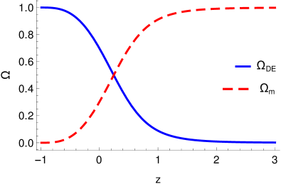
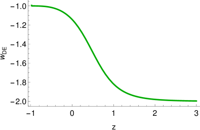
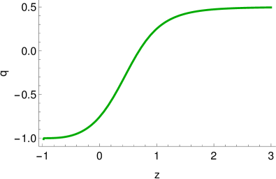
Figure 1: Upper graph: The evolution of the effective dark energy density parameter $\Omega_{DE}$ (blue-solid) and the matter density parameter $\Omega_{m}$ (red-dashed) respectively, as a function of the redshift $z$, for the modified scenario through Kaniadakis entropy, in the case of $\Lambda=0$. Middle graph: The evolution of the effective dark energy equation-of-state parameter $w_{DE}$. Lower graph: Evolution of the deceleration parameter $q$. In all graphs the Kaniadakis entropic parameter is $K=0.35$ in units of $k_{{}_{B}}$, and according to (30) $\Omega_{m0}\approx 0.3$.

In the upper graph of Fig. 1 we present the evolution of the physically accepted energy densities $\Omega_{DE}$ and $\Omega_{m}$ in the case where $K=0.35$ (in units of $k_{B}$), which according to (30) corresponds to $\Omega_{m}(z=0)=\Omega_{m0}\approx 0.30$. As we can see, we acquire the usual thermal history of the Universe, with the sequence of matter and dark-energy epochs, while in the asymptotic future the Universe results in a dark-energy dominated, de Sitter phase. However, the dark-energy equation-of-state parameter $w_{DE}$, although being close to $-1$ at present, and in the future, at large redshifts it goes to $-2$. This behavior is inside the observational bounds Planck:2018vyg , nevertheless it is less attractive. Finally, from the deceleration parameter we can see that the transition from deceleration to acceleration takes place at a redshift $z_{tr}\approx 0.6$, in agreement with observations.

Let us now study in more detail the effect of the entropic parameter $K$ on the cosmic evolution and in particular focusing on the dark energy equation-of-state parameter. In Fig. 2 we depict $w_{DE}$ for different values of $K$. The behavior is similar to the one described above, namely $w_{DE}$ starts from -2, and it becomes around -1 at present and future, while lying always in the phantom regime. Note that the transition redshift has a slight dependence on $K$. Finally, note that in order to have $\Omega_{m0}\approx 0.31\pm 0.014$, which is the $2\sigma$ region according to Planck Collaboration Planck:2018vyg , $K$ is varied in the range $0.3\lesssim K\lesssim 0.45$. Lastly, at asymptotically large times the Universe results always in a dark-energy dominated, de-Sitter phase.

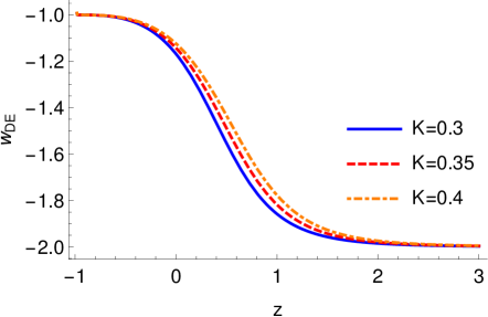
Figure 2: The evolution of the effective dark energy equation-of-state parameter $w_{DE}$, for different values of the Kaniadakis entropic parameter $K$ in unitsof $k_{{}_{B}}$, in the case of $\Lambda=0$. In all cases we have obtained density parameters evolution similar to the graphs of Fig.1, and $\Omega_{m0}$ lies inside the $2\sigma$ region according to Planck Collaboration, namely $\Omega_{m0}\approx 0.31\pm 0.014$ Planck:2018vyg .

III.2 $\Lambda\neq 0$ case

In the previous subsection we examined the case where an explicit cosmological constant is absent, and as we saw the obtained results although in agreement with observation were not completely attractive since the limit $K\rightarrow 0$ could not be obtained and moreover the early-time behavior of $w_{DE}$ was around -2. Hence, in this subsection we consider the case where an explicit cosmological constant is present, namely we consider $\Lambda\neq 0$. In this case, for $K=0$ the scenario does give back $\Lambda$CDM cosmology, nevertheless for $K\neq 0$ the extra terms due to Kaniadakis entropy trigger deviations from $\Lambda$CDM scenario, which is exactly the focus of interest of the present work.

In the upper graph of Fig. 3 we depict the evolution of the energy densities $\Omega_{DE}$ and $\Omega_{m}$, as given by the analytical solution (III) and by $\Omega_{m}(z)=1-\Omega_{DE}(z)$ respectively, in the case where $K=0.2$. Note that we impose $\Omega_{m}(z=0)=\Omega_{m0}\approx 0.3$ in agreement with the Planck results Planck:2018vyg . As we observe, from the resulting evolution of $\Omega_{DE}$ and $\Omega_{m}$ we obtain the usual thermal history of the Universe in agreement with observations, while in the asymptotic future ($z\rightarrow-1$) the Universe results in a dark-energy dominated, de Sitter phase.

Additionally, in the middle graph of Fig. 3 we present the evolution of the dark-energy equation-of-state parameter $w_{DE}$. As can be seen it slightly lies in the phantom regime throughout the Universe evolution, nevertheless still inside the observational bounds Planck:2018vyg , while in the asymptotic future it goes to de Sitter phase as mentioned above. Lastly, in the lower graph we depict the corresponding deceleration parameter $q(z)$. From this plot we can see the transition from deceleration to acceleration at a redshift $z_{tr}\approx 0.6$, in agreement with the observed behavior.

We proceed by examining the effect of the entropic parameter $K$ on the dark energy equation-of-state parameter. In Fig. 4 we present $w_{DE}$ for different values of Kaniadakis parameter $K$. As we stated above, for $K\rightarrow 0$ we re-obtain the $\Lambda$CDM scenario, i.e. $w_{DE}=-1=const.$. As the Kaniadakis parameter increases, the dark energy shows a dynamical behaviour, with $w_{DE}$ at larger redshifts lying slightly in the phantom regime, but at small redshifts and current time it deviates more significantly from $\Lambda$CDM cosmology. Finally, at asymptotically large times, it will always stabilize at the cosmological constant value $-1$, and the Universe always results in the de-Sitter solution, independently of the Kaniadakis parameter $K$. Note that $w_{DE}$ is always in the phantom regime, which is an advantage of the scenario, since it is known that the phantom regime cannot be easily obtained.

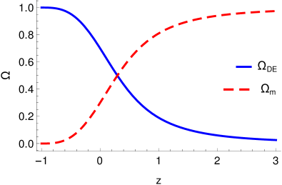
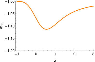
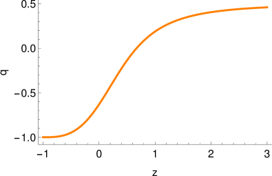
Figure 3: Upper graph: The evolution of the effective dark energy density parameter $\Omega_{DE}$ (blue-solid) and the matter density parameter $\Omega_{m}$ (red-dashed) respectively, as a function of the redshift $z$, for the modified scenario through Kaniadakis entropy. Middle graph: The evolution of the effective dark energy equation-of-state parameter $w_{DE}$. Lower graph: Evolution of the deceleration parameter $q$. In all graphs the Kaniadakis entropic parameter is $K=0.2$ in units of $k_{{}_{B}}$, while $\Lambda$ is given by (25), and we have fixed $\Omega_{m}(z=0)=\Omega_{m0}\approx 0.3$.

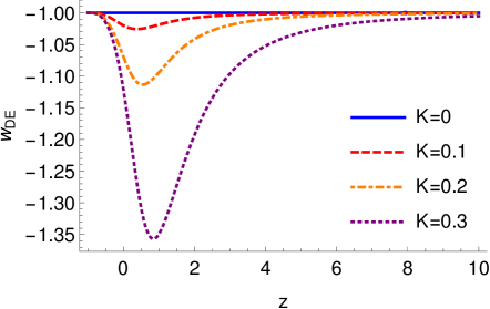
Figure 4: The evolution of the effective dark energy equation-of-state parameter $w_{DE}$, for different values of the Kaniadakis entropic parameter $K$. We have imposed $\Omega_{m0}\approx 0.3$ at present time in units of $k_{{}_{B}}$, and in all cases we have obtained density parameters evolution similar to the graphs of Fig.3.

We close this subsection with the calculation of the Universe age according to the scenario at hand. Starting from the expression $t(z)=\int^{\infty}_{z}\frac{dz^{{}^{\prime}}}{(1+z^{{}^{\prime}})H(z^{{}^{\prime}})}$ and inserting a typical $H(z)$ evolution obtained above we find $t(z)=\frac{0.966279}{H_{0}}$, and thus with the Planck value $H_{0}=(67.27\pm 0.60)$ km/s/Mpc we finally obtain

$$t_{age}=13.936^{+0.017}_{-0.017}\ Gyrs.$$ (31)

This value coincides within 1$\sigma$ with the value corresponding to $\Lambda$CDM scenario, namely $13.787^{+0.020}_{-0.020}$ Gyrs Planck:2018vyg .

III.3 Relation with new Tsallis entropy

For completeness, in this subsection we examine the relation of Kaniadakis entropy with New Tsallis entropy. The latter can be written as

$$S_{T}=\frac{2\exp\left(\frac{\delta S_{BH}}{2}\right)}{\delta}\sinh{\left(\frac{\delta S_{BH}}{2}\right)},$$ (32)

and as it can be seen at small $\delta$ it is quite similar with Kaniadakis entropy (10). Repeating the steps of subsection II.2, but using the above entropy instead of Kaniadakis entropy we obtain the following modified Friedmann equations:

$$\!\!\!\!\!\!\!-4\pi G(\rho_{m}+p_{m})=e^{\frac{\delta\pi}{G(H^{2}+\frac{k}{a^{2}})}}\left(\dot{H}-\frac{k}{a^{2}}\right)$$

$$\!\!\!\!\!\!\!\cdot\left\{\sinh{\left[\frac{\delta\pi}{G(H^{2}+\frac{k}{a^{2}})}\right]}+\cosh{\left[\frac{\delta\pi}{G(H^{2}+\frac{k}{a^{2}})}\right\}}\right].$$ (33)

$$\frac{8\pi G}{3}\rho_{m} = e^{\frac{\delta\pi}{G(H^{2}+\frac{k}{a^{2}})}}\left(H^{2}+\frac{k}{a^{2}}\right)$$ (34)

$$-\frac{\delta\pi}{G}\text{Ei}{\left[\frac{\delta\pi}{G(H^{2}+\frac{k}{a^{2}})}\right]}-\frac{\Lambda}{3},$$

where $\text{Ei}{(x)}$ is defined as $\text{Ei}{(x)}=-\int^{\infty}_{-x}{\frac{e^{-x^{\prime}}}{x^{\prime}}dx^{\prime}}$. Additionally, the effective dark energy density and pressure become

$$\rho_{DE}=\frac{3}{8\pi G}\!\left[\frac{\Lambda}{3}+H^{2}\!\left(1\!-\!e^{\frac{\delta\pi}{GH^{2}}}\right)\!+\frac{\delta\pi}{G}\text{Ei}{\left(\frac{\delta\pi}{GH^{2}}\right)}\!\right],$$ (35)

$$\!\!\!\!\!\!\!\!\!\!\!\!\!\!\!\!\!\!\!\!\!\!\!\!\!\!\!\!\!\!p_{DE}=-\frac{1}{8\pi G}\bigg{[}\Lambda+(3H^{2}+2\dot{H})\left(1-e^{\frac{\delta\pi}{GH^{2}}}\right)$$ (36)

$$\ \ \ \ \,+\frac{3\delta\pi}{G}\text{Ei}{\left(\frac{\delta\pi}{GH^{2}}\right)}\bigg{]}.$$

Expanding the $\text{Ei}(x)$ function for small $\delta$ as $\text{Ei}{(x)}=\gamma+\log(x)+x+\frac{x^{2}}{4}+\dots$, where $\gamma$ is Euler’s constant, we finally obtain

$$\Omega_{DE}=1-\frac{-\mathcal{D}-\mathcal{E}\mathcal{F}+\sqrt{4\mathcal{E}\left(1+\mathcal{E}\right)+\left(\mathcal{D}+\mathcal{E}\mathcal{F}\right)^{2}}}{2\mathcal{E}\left(1+\mathcal{E}\right)},$$ (37)

with

$$\!\!\!\!\!\!\!\!\!\!\!\mathcal{D}=\frac{\Lambda}{3H^{2}_{0}\Omega_{m0}(1+z)^{3}}+1,$$

$$\!\!\!\!\!\!\!\!\!\!\!\mathcal{E}=\frac{\delta\pi}{GH^{2}_{0}\Omega_{m0}(1+z)^{3}},$$

$$\!\!\!\!\!\!\!\!\!\!\!\mathcal{F}=\gamma+\log(\mathcal{E})-2.$$

Lastly, applying the first Friedmann equation at present we extract the relation between the two free parameters $\delta$ and $\Lambda$, namely

$$\!\!\!\!\!\!\!\!\!\!\!\!\Lambda=3H^{2}_{0}(1-\Omega_{m0})-\frac{\delta^{2}\pi^{2}}{G^{2}H^{2}_{0}}$$

$$-\frac{3\delta\pi}{G}\left[\gamma+\log\left({\frac{\delta\pi}{G\Omega_{m0}H^{2}_{0}}}\right)\Omega_{m0}-2\right],$$ (38)

leaving the scenario with one free parameter. Note that for $\delta\rightarrow 0$, all the above obtained equations reduce to the ones of $\Lambda$CDM cosmology.

Elaborating the above equations numerically, we find that the model can indeed describe the thermal history of the Universe, with dark-energy density parameter, deceleration parameter, and dark-energy equation-of-state parameter evolution similarly to Fig. 3. Additionally, in Fig. 5 we display $w_{DE}$ for different values of the Tsallis parameter $\delta$. As we observe, although for $\delta=0$ we recover $\Lambda$CDM scenario, for $\delta$ deviating from zero we obtain a dark-energy sector lying in the quintessence regime, with the deviations from $\Lambda$CDM cosmology being larger at small redshifts. Moreover, at asymptotically large times the dark-energy equation-of-state parameter stabilizes at the cosmological constant value $-1$, and the Universe always results in the de-Sitter solution independently of the Tsallis parameter. Lastly, we mention that, similarly to Kaniadakis case, an explicit cosmological constant is required in order to have efficient phenomenology.

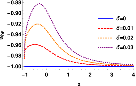
Figure 5: The evolution of the effective dark energy equation-of-state parameter $w_{DE}$, for different values of the new Tsallis entropy parameter $\delta$ in (32), in the case of $\Lambda\neq 0$.

IV Conclusions

In this work we have constructed new cosmological scenarios by considering the widely-known conjecture that thermodynamics is related to gravity. In particular, it is known that one can start from the first law of thermodynamics, applied in the Universe horizon, and result in the Friedmann equations. In this procedure one uses the entropy relation, namely the Bekenstein-Hawking one in the case of General Relativity or the modified entropy expression in the case of modified gravity. Nevertheless, following the above procedure in the reverse way, and applying the generalized Kaniadakis hyperbolic entropy, we extracted modified Friedmann equations, which contain extra terms that appear for the first time. These new terms are quantified by the single, new, Kaniadakis entropy parameter $K$ and effectively give rise to a dark energy sector. In the case $K=0$, where Kaniadakis entropy becomes the standard Bekenstein-Hawking one, the above effective dark energy becomes a constant and $\Lambda$CDM concordance model is re-obtained. However, in the case where deviations of Kaniadakis from Bekenstein-Hawking one are switched on, we acquire very interesting cosmological behavior.

In order to study this behavior in a more thorough way, we assumed the matter sector to be dust, which allowed us to find analytical solutions for the dark energy density parameter, as well as for the dark-energy equation of state and for the deceleration parameter. As we saw, the Universe realizes the sequence of matter and dark-energy epochs, while it transits from deceleration to acceleration at $z_{tr}\approx 0.6$ in agreement with the observed behavior. Furthermore, when we consider an explicit cosmological constant, according to the value of $K$ the equation-of-state parameter of dark energy deviates from the cosmological constant value at small redshifts, while lying always in the phantom regime. Additionally, at asymptotic late times it stabilizes in the cosmological constant value $-1$, i.e. the Universe always results in a dark-energy dominated, de Sitter phase.

For completeness, we investigated the sub-case where there is not an explicit cosmological constant. In this case the scenario at hand does not have $\Lambda$CDM cosmology as a limit, and the evolution is determined solely by the extra terms. We extracted analytical solutions for the dark energy density and we showed that even without $\Lambda$ the new terms can trigger the sequence of matter and dark energy eras. Furthermore, the dark energy equation-of-state parameter starts from -2 at large redshifts, and it becomes around -1 at present and future times, while lying always in the phantom regime, while the transition redshift has a slight dependence on $K$. Note that this $w_{DE}$ behavior is still inside the observational bounds of Planck Collaboration, since the deviation from $-1$ takes place at quite early times, where the observational errors are huge Planck:2018vyg .

In conclusion, the modified cosmology obtained from the gravity-thermodynamics conjecture through Kaniadakis entropy leads to very interesting Universe evolution. It would be both interesting and necessary to perform a full observational analysis using data from Supernova type Ia (SNIa), Baryon Acoustic Oscillation (BAO), Cosmic Microwave Background (CMB), and Hubble parameter measurements, in order to extract constraints on the model parameter $K$. Such an investigation will be performed in a forthcoming publication.

References

- (1) E. N. Saridakis et al. [CANTATA], [arXiv:2105.12582 [gr-qc]].
- (2) S. Capozziello and M. De Laurentis, Phys. Rept. 509, 167 (2011).
- (3) Y. F. Cai, S. Capozziello, M. De Laurentis and E. N. Saridakis, Rept. Prog. Phys. 79, 106901 (2016).
- (4) K. S. Stelle, Phys. Rev. D 16, 953 (1977).
- (5) T. Biswas, E. Gerwick, T. Koivisto and A. Mazumdar, Phys. Rev. Lett. 108, 031101 (2012).
- (6) A. A. Starobinsky, Phys. Lett. B 91, 99 (1980).
- (7) A. De Felice and S. Tsujikawa, Living Rev. Rel. 13, 3 (2010).
- (8) S. Capozziello, Int. J. Mod. Phys. D 11, 483 (2002).
- (9) S. Nojiri and S. D. Odintsov, Phys. Rept. 505, 59 (2011).
- (10) S. Nojiri and S. D. Odintsov, Phys. Lett. B 631, 1 (2005).
- (11) A. De Felice and S. Tsujikawa, Phys. Lett. B 675, 1 (2009).
- (12) D. Lovelock, J. Math. Phys. 12, 498 (1971).
- (13) N. Deruelle and L. Farina-Busto, Phys. Rev. D 41, 3696 (1990).
- (14) P. D. Mannheim and D. Kazanas, Astrophys. J. 342, 635 (1989).
- (15) E. E. Flanagan, Phys. Rev. D 74, 023002 (2006).
- (16) A. Nicolis, R. Rattazzi and E. Trincherini, Phys. Rev. D 79, 064036 (2009).
- (17) C. Deffayet, G. Esposito-Farese and A. Vikman, Phys. Rev. D 79, 084003 (2009).
- (18) G. Leon and E. N. Saridakis, JCAP 1303, 025 (2013).
- (19) G. R. Bengochea and R. Ferraro, Phys. Rev. D 79, 124019 (2009).
- (20) E. V. Linder, Phys. Rev. D 81, 127301 (2010).
- (21) S. H. Chen, J. B. Dent, S. Dutta and E. N. Saridakis, Phys. Rev. D 83, 023508 (2011).
- (22) G. Kofinas and E. N. Saridakis, Phys. Rev. D 90, 084044 (2014).
- (23) G. Kofinas and E. N. Saridakis, Phys. Rev. D 90, 084045 (2014).
- (24) J. Beltrán Jiménez, L. Heisenberg, T. S. Koivisto and S. Pekar, Phys. Rev. D 101, no.10, 103507 (2020).
- (25) F. K. Anagnostopoulos, S. Basilakos and E. N. Saridakis, [arXiv:2104.15123 [gr-qc]].
- (26) S. Basilakos, A. P. Kouretsis, E. N. Saridakis and P. Stavrinos, Phys. Rev. D 88, 123510 (2013).
- (27) K. A. Olive, Phys. Rept. 190, 307 (1990).
- (28) N. Bartolo, E. Komatsu, S. Matarrese and A. Riotto, Phys. Rept. 402, 103 (2004).
- (29) E. J. Copeland, M. Sami and S. Tsujikawa, Int. J. Mod. Phys. D 15, 1753 (2006).
- (30) Y. -F. Cai, E. N. Saridakis, M. R. Setare and J. -Q. Xia, Phys. Rept. 493, 1 (2010).
- (31) E. N. Saridakis, [arXiv:2105.08646 [astro-ph.CO]].
- (32) T. Jacobson, Phys. Rev. Lett. 75, 1260 (1995).
- (33) T. Padmanabhan, Phys. Rept. 406, 49 (2005).
- (34) T. Padmanabhan, Rept. Prog. Phys. 73, 046901 (2010).
- (35) A. V. Frolov and L. Kofman, JCAP 0305, 009 (2003).
- (36) R. G. Cai and S. P. Kim, JHEP 0502, 050 (2005).
- (37) M. Akbar and R. G. Cai, Phys. Rev. D 75, 084003 (2007).
- (38) R. G. Cai and L. M. Cao, Phys. Rev. D 75, 064008 (2007).
- (39) A. Paranjape, S. Sarkar and T. Padmanabhan, Phys. Rev. D 74, 104015 (2006).
- (40) A. Sheykhi, B. Wang and R. G. Cai, Nucl. Phys. B 779, 1 (2007).
- (41) M. Akbar and R. G. Cai, Phys. Lett. B 635, 7 (2006).
- (42) M. Jamil, E. N. Saridakis and M. R. Setare, Phys. Rev. D 81, 023007 (2010).
- (43) R. G. Cai and N. Ohta, Phys. Rev. D 81, 084061 (2010).
- (44) M. Wang, J. Jing, C. Ding and S. Chen, Phys. Rev. D 81, 083006 (2010).
- (45) M. Jamil, E. N. Saridakis and M. R. Setare, JCAP 1011, 032 (2010).
- (46) A. Sheykhi, Phys. Rev. D 81, 104011 (2010).
- (47) A. Sheykhi, Eur. Phys. J. C 69, 265-269 (2010).
- (48) Y. Gim, W. Kim and S. H. Yi, JHEP 1407, 002 (2014).
- (49) Z. Y. Fan and H. Lu, Phys. Rev. D 91, no. 6, 064009 (2015).
- (50) A. Lymperis and E. N. Saridakis, Eur. Phys. J. C 78 (2018) no.12, 993.
- (51) A. Sheykhi, Phys. Lett. B 785, 118-126 (2018).
- (52) E. N. Saridakis, JCAP 07 (2020), 031.
- (53) A. Lymperis, “Cosmological aspects of Unified Theories”. http://hdl.handle.net/10889/14718
- (54) B. D. Sharma, D. P. Mittal,, J. Math. Sci. 10, 28 (1975).
- (55) A. Rényi, Proceedings of the Fourth Berkeley Symposium on Mathematical Statistics and Probability, Volume 1: Contributions to the Theory of Statistics, 547-561, (1961)
- (56) C. E. Shannon, Bell Syst.Tech.J. 27, (1948) 379-423, Bell Syst.Tech.J. 27 (1948) 623-656.
- (57) C. Tsallis, J. Statist. Phys. 52, 479 (1988).
- (58) M. L. Lyra and C. Tsallis, Phys. Rev. Lett. 80, 53 (1998).
- (59) J. D. Barrow, Phys. Lett. B 808, 135643 (2020).
- (60) G. Kaniadakis, Phys. Rev. E 66, 056125 (2002).
- (61) G. Kaniadakis, Phys. Rev. E 72, 036108 (2005).
- (62) R. G. Cai, L. M. Cao and Y. P. Hu, Class. Quant. Grav. 26, 155018 (2009).
- (63) D. Bak and S. J. Rey, Class. Quant. Grav. 17, L83 (2000).
- (64) G. W. Gibbons and S. W. Hawking, Phys. Rev. D 15, 2738 (1977).
- (65) G. Izquierdo and D. Pavon, Phys. Lett. B 633, 420 (2006).
- (66) E. M. C. Abreu, J. Ananias Neto, E. M. Barboza and R. C. Nunes, EPL 114, no.5, 55001 (2016).
- (67) E. M. C. Abreu, J. A. Neto, E. M. Barboza and R. C. Nunes, Int. J. Mod. Phys. A 32, no.05, 1750028 (2017).
- (68) E. M. C. Abreu, J. A. Neto, A. C. R. Mendes and A. Bonilla, EPL 121, no.4, 45002 (2018).
- (69) E. M. C. Abreu, J. A. Neto, A. C. R. Mendes and R. M. de Paula, Chaos, Solitons and Fractals 118, 307-310 (2019).
- (70) W. H. Yang, Y. Z. Xiong, H. Chen and S. Q. Liu, Chin. Phys. B 29, no.11, 110401 (2020).
- (71) U. K. Sharma, V. C. Dubey, A. H. Ziaie and H. Moradpour, [arXiv:2106.08139 [physics.gen-ph]].
- (72) E. M. C. Abreu and J. Ananias Neto, EPL 133, no.4, 49001 (2021).
- (73) N. Drepanou, A. Lymperis, E. N. Saridakis and K. Yesmakhanova, [arXiv:2109.09181 [gr-qc]].
- (74) H. Moradpour, A. H. Ziaie and M. Kord Zangeneh, Eur. Phys. J. C 80, no.8, 732 (2020).
- (75) R. C. Nunes, E. M. Barboza, Jr., E. M. C. Abreu and J. A. Neto, JCAP 08, 051 (2016).
- (76) C. Tsallis and L. J. L. Cirto, Eur. Phys. J. C 73, 2487 (2013).
- (77) N. Aghanim et al. [Planck], Astron. Astrophys. 641, A6 (2020) [erratum: Astron. Astrophys. 652, C4 (2021)].
- (78) K. Mejrhit and R. Hajji, Eur. Phys. J. C 80 (2020) no.11, 1060.
- (79) K. Mejrhit and S. E. Ennadifi, Phys. Lett. B 794 (2019), 45-49.
- (80) K. Ourabah, E. M. Barboza, E. M. C. Abreu and J. A. Neto, Phys. Rev. D 100 (2019) no.10, 103516.
- (81) H. Moradpour, C. Corda, A. H. Ziaie and S. Ghaffari, EPL 127 (2019) no.6, 60006.
- (82) H. Shababi and K. Ourabah, Eur. Phys. J. Plus 135 (2020) no.9, 697.
- (83) J. D. Barrow, S. Basilakos and E. N. Saridakis, Phys. Lett. B 815, 136134 (2021).