Towards Self-Explainable Graph Neural Network

Abstract.

Graph Neural Networks (GNNs), which generalize the deep neural networks to graph-structured data, have achieved great success in modeling graphs. However, as an extension of deep learning for graphs, GNNs lack explainability, which largely limits their adoption in scenarios that demand the transparency of models. Though many efforts are taken to improve the explainability of deep learning, they mainly focus on i.i.d data, which cannot be directly applied to explain the predictions of GNNs because GNNs utilize both node features and graph topology to make predictions. There are only very few work on the explainability of GNNs and they focus on post-hoc explanations. Since post-hoc explanations are not directly obtained from the GNNs, they can be biased and misrepresent the true explanations. Therefore, in this paper, we study a novel problem of self-explainable GNNs which can simultaneously give predictions and explanations. We propose a new framework which can find $K$-nearest labeled nodes for each unlabeled node to give explainable node classification, where nearest labeled nodes are found by interpretable similarity module in terms of both node similarity and local structure similarity. Extensive experiments on real-world and synthetic datasets demonstrate the effectiveness of the proposed framework for explainable node classification.

1. Introduction

Graph neural networks (GNNs) (Bruna et al., 2014; Kipf and Welling, 2016; Hamilton et al., 2017) have made remarkable achievements in modeling graph structured data from various domains such as social networks (Hamilton et al., 2017; Dai and Wang, 2021), financial system (Wang et al., 2019a), and recommendation system (Wang et al., 2019b). The success of GNNs relies on the message-passing. More specifically, the node representations in GNNs will aggregate the information from the neighbors. As a result, the learned representations will capture the node attributes and local topology information to facilitate various tasks, especially the semi-supervised node classification.

Despite the success in modeling graph data, predictions of GNNs are not interpretable for human, which limits the adoption of GNNs in various domains such as credit approval in finance. First, as an extension of deep learning on graphs, the high non-linearity of GNNs makes the predictions difficult to understand. Second, GNNs utilize both node attributes and graph topology to give predictions, which leads to additional challenges to interpret the predictions. Though various approaches (Shu et al., 2019; Papernot and McDaniel, 2018) have been studied to give interpretable predictions or explain trained neural networks, most of them are designed for i.i.d data such as images and cannot handle the relational information. Thus, they cannot be directly applied for GNNs which highly rely on relational information in graphs. Some initial efforts (Ying et al., 2019; Luo et al., 2020; Huang et al., 2020) have been taken to address this problem. For instance, GNNExplainer (Ying et al., 2019) takes a trained GNN and its predictions as inputs and output crucial node attributes and subgraphs to explain the GNN’s predictions. However, all the aforementioned GNN explainers only focus on the post-hoc explanations, i.e., learning an explainer to explain the outputs of a trained GNN. Since the post-hoc explanations are not directly obtained from the GNNs, they can be biased and misrepresent the true explanations of the GNNs. Therefore, it is crucial to develop a self-explainable GNN, which can simultaneously give predictions and explanations.

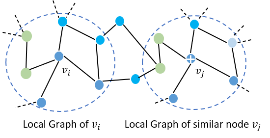
Figure 1. Example of interpretable $K$-nearest labeled nodes

One perspective to obtain the self-explanation for node classification is to identify interpretable $K$-nearest labeled nodes for each node and utilize the $K$-nearest labeled nodes to simultaneously give label prediction and explain why such prediction is given. An example of the interpretable $K$-nearest labeled is shown in Figure 1. As it shows in Figure 1, the topology and node attributes in local graph of node $v_{i}$ are well matched with that of the node $v_{j}$ which is labeled as positive. Thus, $v_{i}$ should be predicted as positive. Then the explaintions can be: (i) “node $v_{i}$ is classified as class $X$ because most of the $K$-nearest labeled nodes of $v_{i}$ belong to class $X$”; and (ii) “node $v_{i}$ is similar to node $v_{j}$ because the n-hop subgraphs centered at these two nodes are similar. For example, this part of the structure and attributes of $v_{i}$’s n-hop subgraph matches to that of $v_{j}$’s”. Though being promising, the work on exploring $K$-nearest neighbors for self-explainable GNNs is rather limited.

Therefore, in this paper, we investigate a novel problem of self-explainable GNN by exploring $K$-nearest labeled nodes. However, developing self-explainable GNN which gives interpretable $K$-nearest labeled nodes is non-trivial. In essense, we are faced with the following challenges: (i) how to incorporate the node similarity and structure similarity to identify $K$-nearest labeled nodes? For graph-structured data, the similarity should take both node attributes and local topology into consideration. Existing works of interpretable deep KNN (Papernot and McDaniel, 2018) mostly focus on i.i.d data and cannot handle the structure similarity. One straightforward solution is using the cosine similarity of node representations learned by GNNs (Kipf and Welling, 2016; Hamilton et al., 2017) to identify the $K$-nearest labeled nodes. But the selection of the $K$-nearest labeled nodes is not interpretable, because the local graph topology and node attributes are implicitly embedded in latent vectors. In addition, ground-truth of node and structure similarity is generally not available. Due to the lack of explicit supervision, it is challenging to identify the true $K$-nearest labeled nodes; and (ii) how to simultaneously give accurate predictions and correct corresponding explanations. The supervision we have is only the labels for classification accuracy. How to leverage label information to help learn the explanations is required to be investigated.

In an attempt to solve the challenges, we propose a model named as Self-Explainable GNN (SE-GNN). SE-GNN adopts a novel mechanism that can explicitly evaluate the node similarity and local structure similarity. For the structure similarity estimation, similarity scores of edges across the local graphs of two nodes will be evaluated to provide self-explanations. The prediction can be supervised by provided labels. And labels can also provide implicit supervision to guide the similarity modeling, because nodes with same labels are more likely to be a similar pair. Therefore, We propose a novel classification loss to simultaneously ensure the accuracy of the prediction and facilitate the interpretable similarity modeling. Furthermore, SE-GNN adopts contrastive learning on node and edge representations to supervise node similarity and edge matching explanations. The main contributions are:

• We study a novel problem of self-explainable GNN by exploring $K$-nearest labeled nodes for predictions and explanations;

• We develop a novel framework SE-GNN, which adopts an interpretable similarity modeling to identify $K$-nearest labeled nodes and enhance the explanations with self-supervision;

• We generate a synthetic dataset to quantitatively evaluate the quality of explanations, i.e., interpretable $K$-nearest labeled nodes, which can facilitate future research in this direction; and

• We conduct extensive experiments on both real-world datasets and synthetic datasets and demonstrate that SE-GNN can give accurate predictions and explanations.

2. Related Work

2.1. Graph Neural Networks

Graph Neural Networks (GNNs) have shown their great power in modeling graph-structure data for various applications such as traffic analysis (Zhao et al., 2020) and drug generation (Bongini et al., 2021). GNNs can be generally split into two categories, i.e., spectral-based (Bruna et al., 2014; Kipf and Welling, 2016; Levie et al., 2018) and spatial-based (Veličković et al., 2018a; Hamilton et al., 2017; Chen et al., 2018; Chiang et al., 2019; Zhao et al., 2021). Spectral-based methods learn the node representations based on spectral graph theory. For example, Bruna et al. (Bruna et al., 2014) first generalize the convolution to graph-structure data with spectral graph theory. To remove the computationally expensive Laplacian eigendecomposition, ChebyNets (Defferrard et al., 2016) define graph convolutions with Chebyshev polynomials. GCN (Kipf and Welling, 2016) further simplifies the convolutional operation. Spatial-based graph convolution is defined in spatial domain, which updates node representations by aggregating their neighbors’ representations (Niepert et al., 2016; Hamilton et al., 2017). For example, GAT (Veličković et al., 2018a) updates the representations of the nodes from the neighbors with an attention mechanism. Moreover, various spatial methods are proposed for further improvements (Chen et al., 2018; Dai et al., 2021; Chen et al., 2020; Tang et al., 2020). For instance, FastGCN (Chen et al., 2018) is proposed to solve the scalability issue.

Recently, some works employ self-supervised learning to graph structured data for better node representations. Various pretext tasks have been explored to benefit the training of GNNs (Sun et al., 2020; Zhu et al., 2020; Jin et al., 2020a). For example, SuperGAT (Kim and Oh, 2021) deploys the edge prediction as self-supervised task to guide the learning of attention. Furthermore, contrastive learning is also widely adopted as the self-supervised task (Sun et al., 2019; Veličković et al., 2018b; Qiu et al., 2020; You et al., 2020). For instance, Qiu et al. (Qiu et al., 2020) design a subgraph instance discrimination to better capture the topology information. The aforementioned methods are inherently different from our proposed SE-GNN as we focus on self-explainable GNNs and the self-supervision is applied to obtain high-quality explanations.

2.2. Explainability of Graph Neural Networks

To address the problem of lacking interpretability, extensive works have been proposed. Explanations in the existing works generally fall into two categories, i.e., self-explainable and post-hoc explanations. Self-explainable models are self-intrinsic, which can simultaneously make predictions and explain the predictions (Alvarez-Melis and Jaakkola, 2018; Hind et al., 2019). For example, Alvarez et al. (Alvarez-Melis and Jaakkola, 2018) propose a rich class of interpretable models where the explanations are intrinsic to the model. Post-hoc explanations use another model or strategy to explain the behavior of a trained model, such as by learning a local approximation with an interpretable model (Ribeiro et al., 2016), computing saliency map (Zeiler and Fergus, 2014), identifying feature importance (Selvaraju et al., 2017; Du et al., 2018; Shrikumar et al., 2017), obtaining prototypes (Koh and Liang, 2017) and exploring meaning of hidden neurons (Yuan et al., 2019).

Despite the great success, the aforementioned approaches are overwhelmingly developed for i.id. data such as images and texts; while the work on interpretable GNNs for graph structured data are rather limited (Ying et al., 2019; Luo et al., 2020; Yuan et al., 2020; Huang et al., 2020). GNNExplainer (Ying et al., 2019) learns soft masks for edges and node features to find the crucial subgraphs and features to explain the predictions. PGExplainer (Luo et al., 2020) applies a parameterized explainer to generate the edge masks from a global view to identify the important subgraphs. GraphLime (Huang et al., 2020) extends the LIME (Ribeiro et al., 2016) to graph neural networks and investigates the importance of different node features for node classification. However, the graph structure information is ignored in GraphLime.

Our work is inherently different from the aforementioned explainable GNN methods: (i) we focus on learning a self-explainable GNN which can simultaneously give predictions and explanations while all the aforementioned are post-hoc explanations. We don’t need additional explainer, which reduces the risk of misrepresenting the true decision reasons of the model; and (ii) we study a novel approach of finding the $K$-nearest labeled nodes in terms of node and structure similarity for classification and explanation.

3. PROBLEM DEFINITION

We use $\mathcal{G}=(\mathcal{V},\mathcal{E},\mathbf{X})$ to denote an attributed graph, where $\mathcal{V}=\{v_{1},...,v_{N}\}$ is the set of $N$ nodes, $\mathcal{E}\subseteq\mathcal{V}\times\mathcal{V}$ is the set of edges, and $\mathbf{X}=\{\mathbf{x}_{1},...,\mathbf{x}_{N}\}$ is the set of node attributes with $\mathbf{x}_{i}$ being the node attributes of node $v_{i}$. $\mathbf{A}\in\mathbb{R}^{N\times N}$ is the adjacency matrix of the graph $\mathcal{G}$, where $\mathbf{A}_{ij}=1$ if nodes ${v}_{i}$ and ${v}_{j}$ are connected; otherwise $\mathbf{A}_{ij}=0$. In the semi-supervised setting, part of the nodes $\mathcal{V}_{L}=\{v_{1},...,v_{l}\}\subset\mathcal{V}$ are labeled. We use $\mathcal{Y}=\{\mathbf{y}_{1},...,\mathbf{y}_{l}\}$ to denote the corresponding labels, where $\mathbf{y}_{i}\in\mathbb{R}^{C}$ is a one-hot vector of node $v_{i}$’s label. $\mathcal{V}_{U}=\mathcal{V}-\mathcal{V}_{L}$ is a set of unlabeled nodes. Most of existing GNNs focus on label prediction of unlabeled nodes in $\mathcal{V}_{U}$ (Wu et al., 2020). They usually lack interpretability on why GNN classifiers give such predictions. There are few attempts of post-hoc explainers (Ying et al., 2019; Luo et al., 2020; Yuan et al., 2020; Huang et al., 2020) to provide explanations for trained GNNs; while the work on self-explainable GNNs is rather limited.

We aim to develop self-explainable GNNs. In particular, for each unlabeled node $v_{i}$, we want to find $K$ most similar labeled nodes with $v_{i}$, and simultaneously utilize these similar nodes to predict $v_{i}$’s label and provide explanation of the prediction. Since both node features and local structure are important for classificaiton, the similarity should be measured in terms of both node features and the n-hop subgraph centered at each node. Sample explanations can be: (i) “node $v_{i}$ is classified as class $B$ because these $K$ nodes have the most similar node features and n-hop subgrph with that of $v_{i}$, and most of these $K$ nodes belong to class $B$”; (ii) “node $v_{i}$ is similar to node $v_{j}$ because the n-hop subgraphs centered at these two nodes are similar. For example, this part of the structure and attributes of $v_{i}$’s n-hop subgraph matches to that of $v_{j}$’s”.

Let $\mathcal{G}_{s}^{(n)}(v_{i})=(v_{i}\cup\mathcal{N}^{(n)}(v_{i}),\mathcal{E}_{s}^{(n)}(v_{i}))$ be the n-hop subgraph centered at node $v_{i}$, where $\mathcal{N}^{(n)}(v_{i})$ is the set of nodes within $n$-hop of $v_{i}$ and $\mathcal{E}_{s}^{(n)}(v_{i})$ is the set of edges that linked the nodes in $\mathcal{G}_{s}^{(n)}(v_{i})$. Let $\mathcal{P}^{(n)}(v_{i},v_{j})\subseteq\mathcal{E}_{s}^{(n)}(v_{i})\times\mathcal{E}_{s}^{(n)}(v_{j})$ be the edge matching result between the local graphs of node $v_{i}$ and $v_{j}$. With these notations, the problem of learning self-explainable GNN by predicting with interpretable $K$-nearest neighbors is defined as:

Problem 1.

Given a graph $\mathcal{G}=(\mathcal{V},\mathcal{E})$ with labeled node set $\mathcal{V}_{L}$ and correspoding label set $\mathcal{Y}$, learn a self-explainable GNN $f_{\mathcal{G}}:\mathcal{G}\rightarrow\mathcal{Y}$ which could give an accurate prediction for each unlabeled node $v_{i}\in\mathcal{V}_{U}$ and simultaneously generate explanation from the $K$-nearest labeled node $\{(v_{ik},\mathcal{G}_{s}^{(n)}(v_{ik}),\mathcal{P}^{(k)}(v_{i},v_{ik}))\}_{k=1}^{K}$, where $v_{ik}\in\mathcal{V}_{L}$ and $\mathcal{G}_{s}^{(n)}(v_{ik})$ are the identified top $K$ nearest labeled nodes and the corresponding $n$-hop subgraph, respectively. $\mathcal{P}^{(n)}(v_{i},v_{ik})$ is the edge matching results between local graphs of $v_{i}$ and $v_{ik}$ to explain the similarity in structure.

4. Methodology

In this section, we present the details of the proposed framework SE-GNN. The basic idea of SE-GNN is: for each node $v_{i}$, it identifies $K$ most similar labeled nodes with $v_{i}$, and utilize the labels of these $K$ nodes to predict $v_{i}$’s label. Meanwhile, the $K$ most similar labeled nodes provide explanations on why such prediction is made in terms of both the structure and feature similarity. There are mainly two challenges: (i) how to obtain interpretable $K$-nearest labeled nodes that consider both node and structure similarity; and (ii) how to simultaneously give accurate predictions and correct corresponding explanations. To address these challenges, SE-GNN explicitly models the node similarity and local structure similarity with explanations. An illustration of the proposed framework is shown in Figure 2. It is mainly composed of an interpretable similarity module and a self-supervisor to enhance the explanations. With the novel similarity modeling process, $K$-nearest labeled nodes of the target node and the similarity explanations can be obtained. Then, prediction of the target node can be given based on the identified $K$-nearest labeled nodes. And, a novel loss function is designed to ensure the accuracy of predictions and facilitate the similarity modeling. Furthermore, self-supervision for explanations is applied to further benefit the accurate explanation generation.

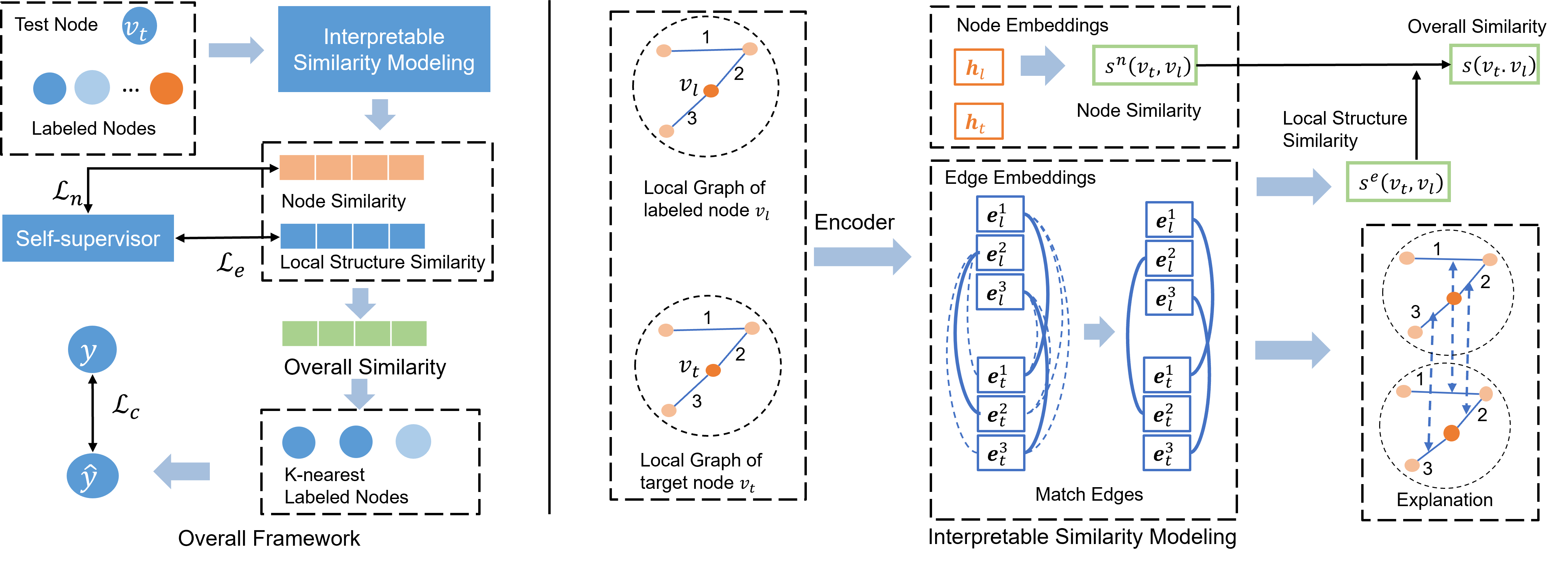
Figure 2. An overview of the proposed SE-GNN.

4.1. Interpretable Similarity Modeling

Since for each node, SE-GNN relies on interpretable $K$-nearest labeled nodes for predictions and explanations, we need to design an interpretable similarity measurements to measure the similarity of nodes. Unlike i.i.d data, which only needs to measure the similarity from the feature perspective, for graph-structure data, both node attributes and the local graph structures of nodes contain crucial information for node classification. Thus, we propose to explicitly model the node similarity and structure similarity to obtain an interpretable overall similarity.

4.1.1. Node Similarity

The node similarity is to evaluate how similar the target node is with the labeled nodes in the node level. Since node features could be noisy and sparse, directly measuring the node similarity in the raw feature space will result in noisy similarity. Following existing work on similarity metric learning (Qiu et al., 2020), we first learn node representations followed by a similarity function, which could better measure node similarity. One straightforward way is to adopt a deep GNN such as GCN (Kipf and Welling, 2016) and GAT (Veličković et al., 2018a) to learn powerful node embeddings. However, current GNNs are found to experience the over-smoothing issue (Li et al., 2018). This may lead to indistinguishable similarity scores for node pairs that actually differ a lot. And a deep GNN may implicitly model the structure information, which could reduce the interpretability of the node similarity. Therefore, we propose to firstly encode the node features with a MLP. Then, the node embeddings are further updated by aggregating the representations from their neighbors with one residual GCN layer (Kipf and Welling, 2016). This process can be mathematically written as:

(1) $$\mathbf{H}^{m}=MLP(\mathbf{X}),\quad\mathbf{H}=\sigma(\tilde{\mathbf{A}}\mathbf{H}^{m}\mathbf{W})+\mathbf{H}^{m},$$

where $\mathbf{X}$ denotes the node attributes, $\tilde{\mathbf{A}}=\mathbf{D}^{-\frac{1}{2}}(\mathbf{A}+\mathbf{I})\mathbf{D}^{-\frac{1}{2}}$ is the normalized adjacency matrix , and $\mathbf{D}$ is a diagonal matrix with $D_{ii}=\sum_{i}A_{ij}$. $\mathbf{I}$ is the identity matrix. $\sigma$ is the activation function such as ReLU. With the learned node embeddings, the node similarity between a target node $v_{t}$ and a labeled node $v_{l}$ can be obtained as:

(2) $$s^{n}(v_{t},v_{l})=sim(\textbf{h}_{t},\textbf{h}_{l}),$$

where $\textbf{h}_{t}$ and $\textbf{h}_{l}$ are the learned embeddings of node $v_{t}$ and $v_{l}$, respectively. $sim$ is flexible to be various similarity metrics such as cosine similarity (You et al., 2020) and distance-based similarity (Plötz and Roth, 2018).

4.1.2. Local Structure Similarity

Generally, the content information, i.e., the n-hop graph structure, is very important for node classification. If two nodes $v_{i}$ and $v_{j}$ have similar $n$-hop subgraphs, their labels are likely to be similar. Thus, in addition to the node level similarity, we also measure the local structure similarity, which can (i) explicitly consider the local structure information to facilitate the identification of $K$-nearest labeled nodes and (ii) provide explanations about the similarity in a structure level. Specifically, we propose to measure how well the edges between the local graphs of two nodes match to evaluate the similarity in structure level. The edge matching results can explain the similarity of two nodes in the aspect of local structure. To match edges for local structure similarity, we need to first learn representations of edges. Since an edge is determined by the two nodes linked by it, for an edge $e=(v_{i},v_{j})$ which links node $v_{i}$ and $v_{j}$, we get the edge representation $\mathbf{e}_{ij}$ as:

(3) $$\mathbf{e}_{ij}=f_{e}(\mathbf{h}_{i},\mathbf{h}_{j}),$$

where $\mathbf{h}_{i}$ and $\mathbf{h}_{j}$ are embeddings of node $v_{i}$ and $v_{j}$, respectively. $f_{e}$ is the function of aggregating the node information to get the edge embedding, which is flexible to various functions such as average pooling and LSTM. In our implementation, we apply average pooling function as $f_{e}$. With Eq.(3), we can get two sets of edge representations $\mathcal{R}_{t}=\{\mathbf{e}_{t}^{1},...,\mathbf{e}_{t}^{M}\}$ and $\mathcal{R}_{l}=\{\mathbf{e}_{l}^{1},...,\mathbf{e}_{l}^{N}\}$ for $\mathcal{E}_{s}^{(n)}(v_{t})$ and $\mathcal{E}_{s}^{(n)}(v_{l})$, where $\mathcal{E}_{s}^{(n)}(v_{t})$ and $\mathcal{E}_{s}^{(n)}(v_{l})$ are the edges in the local graphs of $v_{t}$ and $v_{l}$, respectively. For an edge $e_{t}^{i}\in\mathcal{E}_{s}^{(n)}(v_{t})$, we will find the edge in $\mathcal{E}_{s}^{(n)}(v_{l})$ that matches $e_{t}^{i}$ best. The process of identifying the paired edge for $e_{t}^{i}$ can be formally written as:

(4) $$e_{p}^{i}=\operatorname*{arg\,max}_{e_{l}^{j}\in\mathcal{E}_{s}^{(n)}(v_{l})}sim(\mathbf{e}_{t}^{i},\mathbf{e}_{l}^{j}),$$

where $e_{p}^{i}$ is the found edge in local graph of $v_{l}$ that matches edge $e_{t}^{i}$. The whole edge matching results, which can explain the local structure similarity, can be obtained by:

(5) $$\mathcal{P}^{(n)}(v_{t},v_{l})=\{(e_{t}^{i},e_{p}^{i})\}_{i=1}^{M}.$$

Then, the local structure similarity between $v_{t}$ and $v_{l}$ can be obtained by averaging the similarity scores of all the paired edges:

(6) $$s^{e}(v_{t},v_{l})=\frac{1}{M}{\sum}_{i=1}^{M}sim(\mathbf{e}_{t}^{i},\mathbf{e}_{p}^{i}),$$

where $\mathbf{e}_{p}^{i}$ is the representation of edge $e_{p}^{i}$.

4.1.3. Overall Similarity

With the node similarity and local structure similarity between node $v_{t}$ and $v_{l}$, the overall similarity is:

(7) $$s(v_{t},v_{l})=\lambda s^{n}(v_{t},v_{l})+(1-\lambda)s^{e}(v_{t},v_{l}),$$

where $\lambda$ is a positive scalar to balance the contributions of node similarity and structure similarity.

4.2. Self-Explainable Classification

With the similarity metric described in Section 4.1, we are able to identify the interpretable $K$-nearest labeled nodes to predict and explain the label of the target node. Next, we introduce the details of the prediction process, discussions about the explanations, and the loss function that ensures classification accuracy.

4.2.1. Prediction with K-nearest Labeled Nodes

Let $\mathcal{K}_{t}=\{v_{t}^{1},...,v_{t}^{K}\}$ be the set of $K$-nearest labeled nodes of the target node $v_{t}$ based on Eq.(7). Intuitively, the more similar $v_{t}$ and $v_{t}^{i}$ are, i.e., the larger $s(v_{t},v_{t}^{i})$ is, the more likely $v_{t}$ has the same label as $v_{t}^{i}$. Thus, following deep KNN (Plötz and Roth, 2018; Ren et al., 2014), we predict the label of node $v_{t}$ as weighted average of the labels of the $K$-nearest neighbors. Specifically, the weight $a_{ti}$ of the $i$-th nearest labeled node, i.e., $v_{t}^{i}$, is calculated as

(8) $$a_{ti}=\frac{\exp(s(v_{t},v_{t}^{i})/\tau)}{\sum_{i=1}^{K}\exp(s(v_{t},v_{t}^{i})/\tau)},$$

where $\tau$ is the temperature parameter. With the weight $a_{ti}$, the label of $v_{t}$ is predicted as

(9) $$\hat{\mathbf{y}}_{t}={\sum}_{i=1}^{K}a_{ti}\cdot\mathbf{y}_{t}^{i},$$

where $\mathbf{y}_{t}^{i}$ is the one-hot label vector of $v_{t}^{i}$.

4.2.2. Explanation

For a target node $v_{t}$, the found $K$-nearest labeled nodes $\mathcal{K}_{t}=\{v_{t}^{1},...,v_{t}^{K}\}$ and the corresponding similarity scores $\{s(v_{t},v_{t}^{i})\}_{i=1}^{K}$ can clearly explain the predictive label. For the overall similarity $s(v_{t},v_{t}^{i})$, the contributions of node and structure similarity can be given through $s^{n}(v_{t},v_{t}^{i})$ and $s^{e}(v_{t},v_{t}^{i})$. Moreover, we can track back the identified edge pairs $\mathcal{P}^{(n)}(v_{t},v_{t}^{i})$ between local graph of $v_{t}$ and its $i$-th nearest labeled node $v_{t}^{i}$ to explain the local structure similarity. Though our SE-GNN focuses on explaining the predictions with $K$-nearest labeled nodes, it also can extract the crucial subgraph for explanation. For a crucial edge, the local graphs of $K$-nearest neighbors should also contain similar one. Thus, the importance of an edge $e_{t}^{i}\in\mathcal{E}_{s}^{(n)}(v_{t})$ can be evaluated by its average similarity with the identified pair edges $\{e_{p}^{ij}\}_{j=1}^{K}$ in the local graphs of the $K$-nearest labeled nodes as

(10) $$p(e_{t}^{i})=\frac{1}{K}{\sum}_{j=1}^{K}sim(\mathbf{e}_{t}^{i},\mathbf{e}_{p}^{ij}),$$

where $\mathbf{e}_{t}^{i}$ and $\mathbf{e}_{p}^{ij}$ are edge representations of $e_{t}^{i}$ and $e_{p}^{ij}$, respectively. Then, a threshold can be set to filter out the unimportant edges in the local graph of node $v_{t}$.

4.2.3. Classification Loss

SE-GNN is expected to give accurate predictions. Therefore, we utilize the supervision from the given labels to ensure the accuracy of the self-explainable GNN. One straightforward way is to optimize the predictions of nodes with labels in a leave-one-out manner. More specifically, for a labeled node $v_{i}\in\mathcal{V}_{L}$, we identify $K$-nearest labeled nodes from other labeled nodes $\mathcal{V}_{L}-\{v_{i}\}$. Then loss such as cross entropy loss can be applied to optimize the model. However, in this way, the optimization only involves the searched $K$-nearest neighbors which are generally similar nodes. Lacking of various negative samples may negatively affect similarity modeling. In addition, the computational cost to identify $K$-nearest neighbors will be large when numerous labeled nodes are given. To address these issues, we propose a loss function that adopts negative sampling (Mikolov et al., 2013) and approximately select $K$-nearest labeled nodes as positive samples. Specifically, for a target node $v_{t}\in\mathcal{V}_{L}$, we randomly sample $Q$ labeled nodes $\mathcal{V}_{n}^{t}$ which do not share the same label with $v_{t}$ as negative samples. And we randomly sample $N$ ($N>K$) labeled nodes sharing the same label with $v_{t}$ as support set to obtain approximate $K$-nearest labeled nodes $\tilde{\mathcal{K}}_{t}$. The objective function can be formally written as:

(11) $$\min_{\theta}\mathcal{L}_{c}=\frac{1}{|\mathcal{V}_{L}|}\sum_{v_{t}\in\mathcal{V}_{L}}-\log\frac{\sum_{\tilde{v}_{t}^{i}\in\tilde{\mathcal{K}}_{t}}\exp(s(v_{t},\tilde{v}_{t}^{i})/\tau)}{\sum_{v_{n}^{i}\in\tilde{\mathcal{K}}_{t}\cup\mathcal{V}_{n}^{t}}\exp(s(v_{t},v_{n}^{i})/\tau)},$$

where $\theta$ denotes the parameters of SE-GNN, and $\tau$ is the temperature hyperparameter. With loss function Eq.(11), the similarity scores of node pairs with different labels will be minimized, and the similarity scores between a node and its approximate k-nearest neighbor with the same labels will be maximized. As a result, accurate predictions can be given. Moreover, it provides supervision to guide the similarity modeling. Note that this sampling strategy to obtain approximate $K$-nearest labeled nodes is only applied during the training phase. For testing phase, $K$-nearest labeled nodes are identified from the whole labeled node set $\mathcal{V}_{L}$ and the label is predicted with Eq.(9).

4.3. Enhance Explanation with Self-Supervision

Although the labels can provide the supervision to facilitate the similarity modeling with objective function in Eq.(11), they do not explicitly supervise the node similarity and local structure similarity. In addition, the edge matching results and identification of nearest labeled nodes may not generalize well to unlabeled nodes, because unlabeled nodes are not involved in Eq.(11). To further benefit the explanation generation and similarity metric learning, we adopt a contrastive pretext task to provide self-supervision for node similarity and local structural similarity learning.

Recently, contrastive learning has shown to be effective for unsupervised representation learning on graphs (Veličković et al., 2018b; Qiu et al., 2020; You et al., 2020). Essentially, contrastive learning aims to maximize representation consistency under differently augmented views. In other words, with contrastive learning, similar nodes/graphs will be given similar representations. Therefore, we adopt contrastive learning on node representations to facilitate the node similarity modeling. Moreover, the explanation for local structure similarity relies on accurate edge machining. To guide the edge matching on unlabeled nodes, a contrastive task on edge representations is deployed as well. In detail, we maximize the the agreement between two augmented views of the graphs via a contrastive loss in node and edge representations. Following GraphCL (You et al., 2020), two augmentations, i.e., attribute masking and edge perturbation, are applied to obtain representations from different views. We apply infoNCE loss (Oord et al., 2018) as the contrastive loss. The infoNCE loss transfers the mutual information maximization to a classification task which requires positive pairs and negative pairs. Representations of the same node/edge from these two views will compose positive pairs for contrastive learning. And representations of different nodes in both views compose negative pairs. The contrastive learning is trained in a minibatch manner. For a query representation $\mathbf{h}_{i}$, a dictionary $\{\tilde{\mathbf{h}}_{0},...,\tilde{\mathbf{h}}_{Q_{N}}\}$ which contains one positive sample $\tilde{\mathbf{h}}_{+}$ will be built. The objective function of contrastive learning on node representations can be formulated as:

(12) $$\min_{\theta}\mathcal{L}_{n}=\frac{1}{|\mathcal{V}_{B}|}\sum_{v_{i}\in\mathcal{V}_{B}}-\log\frac{\exp(sim(\mathbf{h}_{i},\tilde{\mathbf{h}}_{+})/\tau)}{\sum_{j=0}^{Q_{N}}\exp(sim(\mathbf{h}_{i},\tilde{\mathbf{h}}_{j})/\tau)}.$$

Similarly, contrastive learning is adopted on the edge representations to benefit the edge matching explanations. Let $\mathcal{E}_{B}$ denotes a minibatch of edges. The objective function can be written as:

(13) $$\min_{\theta}\mathcal{L}_{e}=\frac{1}{|\mathcal{E}_{B}|}\sum_{e_{i}\in\mathcal{E}_{B}}-\log\frac{\exp(sim(\mathbf{e}_{i},\tilde{\mathbf{e}}_{+})/\tau)}{\sum_{j=0}^{Q_{E}}\exp(sim(\mathbf{e}_{i},\tilde{\mathbf{e}}_{j})/\tau)},$$

where $\mathbf{e}_{i}$ denotes a query edge representation, and $\tilde{\mathbf{e}}_{+}$ is the positive sample from dictionary $\{\tilde{\mathbf{e}}_{0},...,\tilde{\mathbf{e}}_{Q_{E}}\}$. With the self-supervision, the representations of similar edges and nodes will be similar, which can facilitate the similarity modeling for explanations. Moreover, since edge perturbation is used to augment the graph in contrastive learning, the representations from the perturbed graph will be enforced to be consistent with the representations from the clean graph. This will lead to robustness against structure noise.

4.4. Overall Objective Function

With the supervision from the labels for accurate prediction, and the contrastive learning on node and edge representations to facilitate the modeling of similarity, the final loss function of SE-GNN is:

(14) $$\min_{\theta}\mathcal{L}_{c}+\alpha\mathcal{L}_{n}+\beta\mathcal{L}_{e},$$

where $\theta$ represents the parameters of SE-GNN. $\alpha$ and $\beta$ are hyperparameters that control the contributions of self-supervision on node similarity modeling and edge matching in local similarity evaluation, respectively.

4.5. Training Algorithm and Time Complexity

4.5.1. Training Algorithm

The training algorithm of SE-GNN is given in Algorithm 1. In line 1, the parameters of SE-GNN are randomly initialized with Xavier initialization (Glorot and Bengio, 2010). In line 3, the supervised loss from the labeled nodes is calculated. Graph augmentation is conducted in line 4, which gives graphs in different views for contrastive learning. From line 5 to line 9, contrastive losses for nodes and edges are computed. For the size of negative samples in Eq.(11), it is fixed as 20. The sizes of negative samples in Eq.(12) and Eq.(13) are both set as 100 during the training phase.

0:  $\mathcal{G}=(\mathcal{V},\mathcal{E},\mathbf{X})$ , $\mathcal{Y}$, $K$, $\alpha$, $\beta$, $\lambda$, $\tau$.

0:  Self-explainable GNN $f_{\mathcal{G}}$.

1:  Randomly initialize the parameters of $f_{\mathcal{G}}$.

2:  repeat

3:     Obtain the classification loss by Eq.(11)

4:     Augment the $\mathcal{G}$ with attribute masking and edge perturbation to receive graphs in different views

5:     Sample a node batch $\mathcal{V}_{B}$ with positive and negative pairs

6:     Calculate contrastive loss on nodes by Eq.(12)

7:     Sample an edge batch $\mathcal{E}_{B}$ with positive and negative pairs

8:     Get contrastive loss on edges by Eq.(13)

9:     Optimize the parameter of $f_{\mathcal{G}}$ by Eq.(14)

10:  until convergence

11:  return  $f_{\mathcal{G}}$

Algorithm 1 Training Algorithm of SE-GNN.

4.5.2. Time Complexity

During the test phase, the main time complexity comes from the similarity scores calculation between the test node $v_{t}$ and all the labeled nodes $\mathcal{V}_{L}$. For each node $v_{l}\in\mathcal{V}_{L}$, the cost for calculating the edge matching with $v_{t}$ is $\mathcal{O}(d\cdot|\mathcal{E}_{t}|\cdot|\mathcal{E}_{l}|)$, where $d$ is the embedding dimension. Thus, the time complexity for one test node is approximately $\mathcal{O}(d\cdot|\mathcal{E}_{t}|\cdot\sum_{v_{l}\in\mathcal{V}_{L}}|\mathcal{E}_{l}|)$. As for the training phase, we adopt a sampling strategy in Eq.(11) to reduce the pairs of similarity to be computed. For each node $v_{t}\in\mathcal{V}_{L}$, let $\mathcal{S}_{t}=\mathcal{K}_{t}\cup\mathcal{V}_{n}^{t}$ denotes the sampled positive and negative nodes in Eq.(11), the cost of calculating classification loss for $v_{t}$ is $\mathcal{O}(d\cdot|\mathcal{E}_{t}|\cdot\sum_{v_{l}\in\mathcal{S}_{t}}\cdot|\mathcal{E}_{l}|)$. Thus, the cost for classification loss of all labeled nodes is $\mathcal{O}(\sum_{v_{t}\in\mathcal{V}_{t}}\sum_{v_{l}\in\mathcal{S}_{t}}d\cdot|\mathcal{E}_{t}|\cdot|\mathcal{E}_{l}|)$.With the computation cost on contrastive learning, the overall time complexity for an iteration in the training phase is $\mathcal{O}(d\cdot(Q_{n}|\mathcal{V}_{B}|+Q_{e}|\mathcal{E}_{B}|+\sum_{v_{t}\in\mathcal{V}_{t}}\sum_{v_{l}\in\mathcal{S}_{t}}|\mathcal{E}_{t}|\cdot|\mathcal{E}_{l}|))$.

5. experiments

In this section, we conduct extensive experiments on real-world and synthetic datasets to demonstrate the effectiveness of SE-GNN. In particular, we aim to answer the following research questions:

• RQ1 Can our proposed method simultaneously provide accurate predictions and corresponding reasonable explanations?

• RQ2 Is SE-GNN robust to the structure noises in the datasets?

• RQ3 How does each component of our proposed SE-GNN contribute to the classification performance and explainability?

5.1. Datasets

To quantitatively and qualitatively evaluate SE-GNN in predictions and explanations, we conduct extensive experiments on three real-world datasets and two synthetic datasets. The statistics of the datasets are presented in Table 1.

5.1.1. Real-World Datasets

To demonstrate the effectiveness of our proposed methods, for real-world datasets, we choose three widely used benchmark networks, i.e., Cora, Citeseer, and Pubmed (Sen et al., 2008). For Cora and Pubmed, the standard dataset splits as in the cited paper are applied. As for Citeseer, it contains isolated nodes which are not applicable to our method. Therefore, following the pre-processing strategy in (Jin et al., 2020b), we select the largest connected component in the Citeseer graph and apply the same dataset splits.

5.1.2. Synthetic Datasets

We construct two synthetic datasets, i.e., Syn-Cora and BA-Shapes, which provide ground truth of explanations for quantitative analysis. The details are described below.

Syn-Cora: This dataset is synthesized from the Cora graph which provides ground-truth of explanations, i.e., $K$-nearest labeled nodes and edge machining results. To construct the graph, motifs are obtained by sampling local graphs of nodes from Cora. Various levels of noises are applied to the motifs in attributes and structures to generate similar local graphs. For a motif and it’s corresponding perturbed versions provide the groundtruth $K$-nearest neighbors and the corresponding edge-matching. Specifically, we sample three motifs for each class, resulting in 21 unique motifs in total. To link the synthetic local graphs together, a subgraph of Cora that have no overlap with the motifs is sampled as the basis graph. These synthetic local graphs are attached to the basis graph by randomly linking three nodes. To simulate a realistic training scenario, we randomly select 30% nodes from the motifs and basis graph as the training set. Testing is conducted on the remaining nodes in the motifs for explanation accuracy evaluation.

BA-Shapes: To compare with the state-of-the-art GNN explainers (Ying et al., 2019; Luo et al., 2020) which identify crucial subgraphs for predictions, we construct BA-Shapes following the setting in GNNExplainer (Ying et al., 2019). BA-Shapes is a single graph consisting of a base Barabasi-Albert (BA) graph with 300 nodes and 80 “house”-structured motifs. These motifs are attached to the BA graph. And random edges are added to perturb the graph. Node features are not assigned in BA-Shapes. Nodes in the base graph are labeled with 0. Nodes locating at the top/middle/bottom of the “house” are labeled with 1,2,3, respectively. Dataset split is the same as that in (Ying et al., 2019).

Table 1. Statistics of datasets.

	Nodes	Edges	Features	Classes
Cora	2,708	5,429	1,433	7
Citeseer	2,110	3,668	3,703	6
Pubmed	19,171	44,338	500	3
Syn-Cora	1,677	4,610	1,433	7
BA-Shapes	700	4,421	-	4

Table 2. Node classification accuracy (%) on real-world datasets.

Dataset	GCN	GIN	SuperGAT	Pro-GNN	MLP-K	GCN-K	GIN-K	Ours
Cora	80.8$\pm 1.1$	80.5$\pm 0.8$	82.4$\pm\mathbf{0.7}$	79.1$\pm 0.1$	53.9$\pm 1.8$	78.8$\pm 1.2$	78.8$\pm 0.3$	80.4$\pm 0.3$
Citeseer	71.9$\pm 1.0$	72.5$\pm 0.8$	73.6$\pm 0.2$	73.3$\pm 0.7$	61.6$\pm 1.6$	71.4$\pm 0.8$	69.2$\pm 1.2$	73.8$\pm\mathbf{0.6}$
Pubmed	78.4$\pm 0.4$	78.9$\pm 0.2$	79.2$\pm 0.4$	79.4 $\pm 0.4$	73.2$\pm 0.2$	77.4$\pm 0.2$	78.8$\pm 0.3$	80.0$\pm\mathbf{0.2}$

5.2. Experimental Settings

5.2.1. Baselines

To evaluate the performance and robustness of SE-GNN in node classification on real-world datasets, we first compare with the following representative and state-of-the-art GNNs, self-supervised GNN, and robust GNN.

• GCN (Kipf and Welling, 2016): GCN is a popular spectral-based GNN which defines graph convolution with spectral theory.

• GIN (Xu et al., 2018): Compared with GCN, multi-layer perception is used in GIN to process the aggregated information from the neighbors in each layer to learn more powerful representations.

• SuperGAT (Kim and Oh, 2021): This is a self-supervised graph neural network. Edge prediction is deployed as the pretext task to directly guide the learning of attention to facilitate the information aggregation.

• Pro-GNN (Jin et al., 2020b): This is state-of-the-art GNN against noisy edges in graphs. It applies low-rank and sparsity constraint to directly learn a clean graph close to the noisy graph to defend against adversarial attacks.

Existing work that identifies the $K$-nearest labeled nodes is rather limited. Therefore, we compare with the following baselines based on the deep KNN (Papernot and McDaniel, 2018) on i.i.d data to evaluate our explanations.

• MLP-K: Following (Papernot and McDaniel, 2018), we first train a MLP with the node features and labels. After training, the node representations from the final layer of MLP is used to find the $K$-nearest labeled nodes. The final prediction of an unlabeled node is obtained using weighted average of the its $K$-nearest labeled nodes.

• GCN-K: Similar to MLP-K, we use the representations from the final layer of GCN to get $K$-nearest neighbors and predictions. Post-hoc explanations in structure similarity can be obtained by edge matching through the edge representations. Edge representations are average representations of the linked nodes .

• GIN-K: It replaces the backbone in GCN-K with GIN to obtain the predictions and explanations.

Finally, we compare with the state-of-the-art GNN explainers in extracting important subgraphs to explain predictions:

• GNNExplainer (Ying et al., 2019): GNNExplainer takes a trained GNN and the predictions as input to obtain post-hoc explanations. It learns a soft edge mask for each instance to identify the crucial subgraph.

• PGExplainer (Luo et al., 2020): It adopts a MLP-based explainer to obtain the important subgraphs from a global view to reduce the computation cost and obtain better explanations.

5.2.2. Implementation Details

The local structure similarity is based on 2-hop local graphs of nodes in all the experiments. For SE-GNN, the encoder consists of two MLP layers and one GCN layer with residual connection. The hidden dimension is set as 64 in these MLP and GCN layers. The rate of attribute masking in the contrastive learning is set as 0.2. We replace 10% edges in the graph to noisy edges for edge perturbation. For experiments on real-world datasets, all hyperparameters are tuned based on the prediction results on the validation set. We vary $\alpha$ and $\beta$ among $\{0.0001,0.001,0.01,0.1,1\}$. The $\lambda$ which balance the node similarity and structure similarity is set as 0.5 for all datasets. The number of nearest labeled nodes used for prediction, i.e., $K$, is set as searched as $\{25,40,50\}$ for all the datasets. The temperature hyperparameter $\tau$ is fixed as 1 in all experiments. For the hyperparameters on the Syn-Cora and BA-Shapes, we reuse the setting on the Cora graph. The BA-shapes dataset does not provide features, we initialize the node features with node degree and number of involved triangles. The hyparameters for the baselines are also tuned on the validation set. All the experiments are conducted 5 times and the average results with standard deviations are reported.

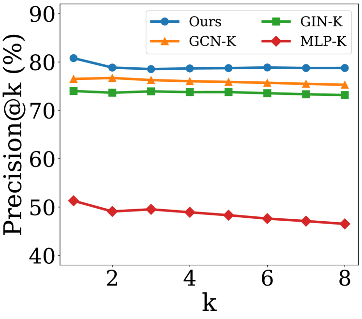
(a) Cora

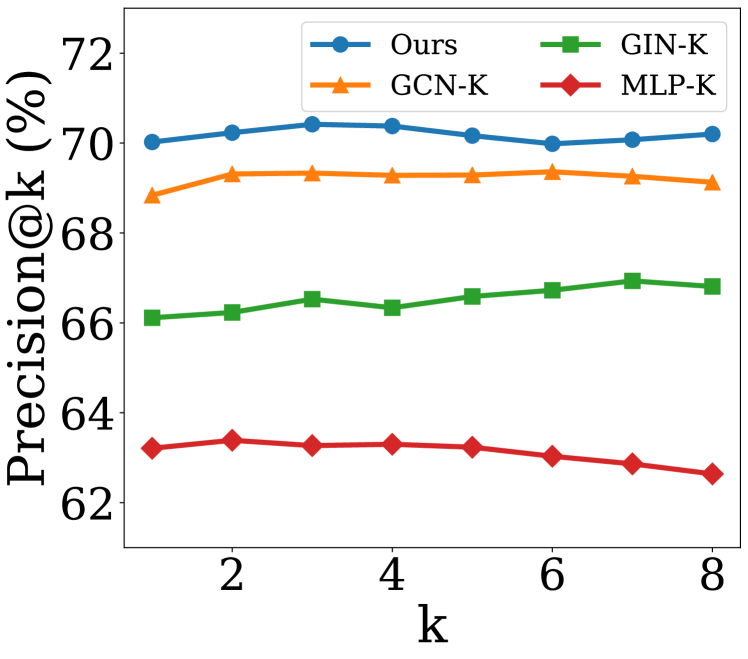
(b) Citeseer

(c) Pubmed

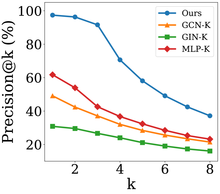
(d) Syn-Cora

Figure 3. The precision@k of the $K$-nearest labeled nodes.

5.3. Classification and Explanation Quality

To answer RQ1, we compare SE-GNN with baselines on real-world datasets and synthetic datasets in terms of classification performance and explanation quality.

5.3.1. Results on Real-World Datasets

To demonstrate that our SE-GNN can give accurate predictions, we compare with the state-of-the-art GNNs on real-world datasets. Each experiment is conducted 5 times. The average node classification accuracy and standard deviations are reported in Table 2. From the table, we observe:

• Our method outperforms GCN and GIN on various real-world datasets especially on the large dataset. This is because information from numerous unlabeled nodes is leveraged in SE-GNN through the similarity modeling with contrastive learning.

• SE-GNN achieves comparable performance with self-supervised method SuperGAT. Note that encoder in SE-GNN only involves 1-hop neighbors to learn representations. This indicates that the designed local structure similarity manages to capture the complex structure information for node classification.

• Though GCN-K and GIN-K also utilize GNN to learn representation and $K$-nearest neighbors for prediction, SE-GNN performs much better than them, which shows the effectiveness of SE-GNN in utilizing the label information and contrastive learning for learning better representations and similarity metrics.

Intuitively, for each test node $v_{t}\in\mathcal{V}_{U}$, SE-GNN should assign higher similarity score to labeled nodes of the same class as $v_{t}$. To analyze this, for each $v_{t}$, we first rank the labeled nodes based on similarity scores. Then We treat the label of $v_{t}$ as the groundtruth and calculate the precision@k for the ranked list. We average the results for all $v_{t}\in\mathcal{V}_{U}$. Generally, if a method assigns higher similarity scores to labeled nodes of the same class as $v_{t}$, it would have large precision@k. We vary $k$ as $\{1,2,\dots,8\}$. The hyperparameters are set as described in Section 5.2.2. The results on the three real-world datasets are presented in Figure 3(a), 3(b) and  3(c), respectively. We can observe that SE-GNN consistently outperforms other baselines by a large margin, which indicates that SE-GNN can retrieve reliable $K$-nearest labeled nodes for prediction and explanation.

Table 3. Average ratings of human evaluation.

Dataset	MLP-K	GCN-K	GIN-K	Ours
Cora	0.030	0.405	0.207	0.763
Citeseer	0.030	0.311	0.326	0.733
Pubmed	0.089	0.348	0.252	0.674

We also conduct qualitative evaluation on explanations on real-world datasets. The explanations of an instance from Citeseer are presented in Figure 4. Specifically, the local graphs of nearest labeled nodes identified by different methods are presented. And we apply t-SNE to node features to obtain the positions of nodes in the visualized graph for node similarity comparison. The shapes of the graphs can help to assess the similarity of local structures. From the Figure 4, we can observe that SE-GNN can correctly identify the labeled node whose features and local topology are both similar with the target node. And the given edge matching results well explain the local structure similarity. On the other hand, baselines fail to identify the similar labeled nodes and provide poor explanations in structure similarity.

To further testify the quality of our explanations, 30 annotators are asked to rate the model’s explanations on three real-world datasets. The explanations are presented in the same way as Fig. 4. Each annotator rates explanations at least 15 instances from the three real-world datasets. The rating score is either 0 (similar) or 1 (disimialr). The average ratings are presented in Table3. From the table, we can find that the nearest neighbors identified by our method receive the highest ratings, which shows that our explanations are in line with the human’s decisions. It verifies the quality of our explanations on real-world datasets.

Table 4. Results on Syn-Cora.

Metric (%)	MLP-K	GCN-K	GIN-K	Ours
Accuracy	93.8$\pm 2.3$	94.8$\pm 0.7$	94.6$\pm 0.7$	97.7$\pm\mathbf{1.6}$
Edge ACC	-	25.1$\pm 0.4$	18.2$\pm 1.8$	81.1$\pm 1.1$

Table 5. Structure explanation AUC on BA-Shapes.

GNNExplainer	PGExplainer	Ours
95.6$\pm 3.7$	98.7$\pm 2.1$	98.1$\pm 0.5$

5.3.2. Results on Syn-Cora

We compare with baselines on Syn-Cora which provides the ground-truth explanations to quantitatively evaluate the two-level explanations, i.e., $K$-nearest labeled nodes and the edge matching results for similarity explanation. The prediction performance is evaluated by accuracy. Precision@k is used to show the quality of $K$-nearest labeled nodes. The accuracy of matching edges (Edge ACC) is used to demonstrate the quality of local structure similarity explanation. The results are presented in Table 4 and Figure 3(d). Note that edge matching is not applicable for MLP-K, because it cannot capture structure information. From the table and figure, we observe:

• Though GCN-K and GIN-K achieve good performance in classification, they fail to identify the true similar nodes and explain the struck similarity. This is due to the over-smoothing issue in deep GNNs, which leads representations poorly persevere similarity information. By contrast, SE-GNN achieves good performance in all explanation metrics, which shows node similarity and local structure similarity are well modeled in SE-GNN.

• Compared with MLP-K which does not experience over-smoothing issue, SE-GNN can give more accurate explanations. This is because we apply the supervision from labels and self-supervision to guide the learning of two-level explanations.

5.3.3. Results on BA-Shapes

As it is discussed in Section 4.2.2, our SE-GNN can be extended to extract a crucial subgraph of the test node’s local graph to explain the prediction. To demonstrate the effectiveness of extracting crucial structures as explanations, we compare SE-GNN with state-of-the-art GNN explainers on a commonly used synthetic dataset BA-Shapes. Following (Ying et al., 2019), crucial structure explanation AUC is used to assess the performance in explanation. The average results of 5 runs are reported in Table 5. From this table, we can observe that, though SE-GNN is not developed for extracting crucial subgraph for providing explanations, our SE-GNN achieves comparable explanation performance with state-of-the-art methods. This implies that accurate crucial structure can be derived from the SE-GNN’s explanations in local structure similarity, which further demonstrates that our SE-GNN could give high-quality explanations.

Figure 4. Illustration of the explanation from SE-GNN and other baselines. Node colors denote the label of nodes. Edges with the same number denote that they are matched.

5.4. Robustness

Structure noises widely exist in the real world and can significantly degrade the performance of GNNs (Zügner et al., 2018; Zügner and Günnemann, 2019). SE-GNN adopts graph topology in representations learning and local similarity evaluation, which could be affected by noisy edges. Therefore, we conduct experiments on noisy graphs to evaluate the robustness of SE-GNN to answer RQ2. Experiments are conducted on two types of noisy graphs, i.e., graphs with random noise and non-targeted attack perturbed graphs. For non-targeted attack, we apply metattack (Zügner et al., 2018), which poisons the structure of the graphs via meta-learning. The perturbation rate of non-targeted attack and random noise is varied as $\{0\%,5\%,\dots,25\%\}$. The results on Citeseer are shown in Figure 5. From this figure, we observe that SE-GNN outperforms GCN by a large margin when the perturbation rates are higher. For example, SE-GNN achieves over 10% improvements when the perturbation rate of metattack is 25%. And SE-GNN even performs better than Pro-GNN which is one of the state-of-the-art robust GNNs against structure noise. This is because:(i) The contrastive learning in SE-GNN encourages the representations consistency between the clean graph and randomly perturbed graph. Thus, the learned encoder will not be largely affected by structure noises; (ii) Noisy edges link the nodes that are rarely linked together. Thus, the noise edges generally receive low similarity scores and would not be selected to compute local structure similarity.

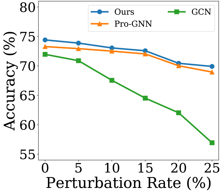
(a) Metattack

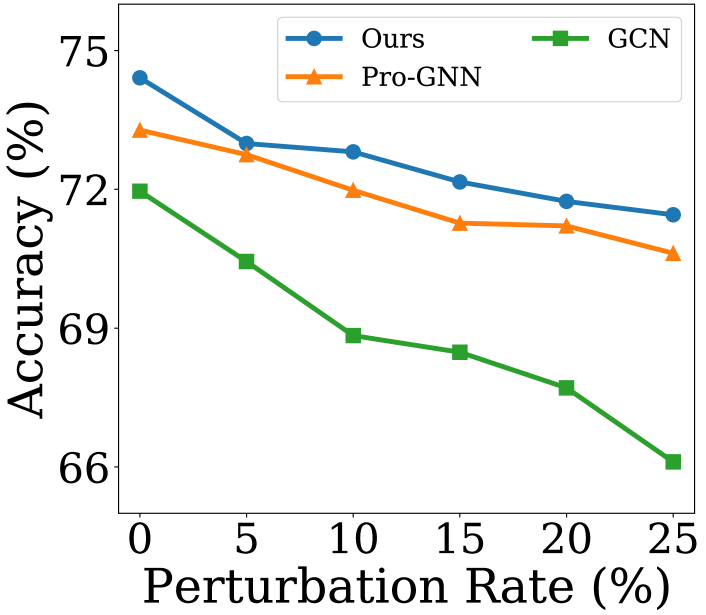
(b) Random Noise

Figure 5. Robustness under different Ptb rates on Citeseer.

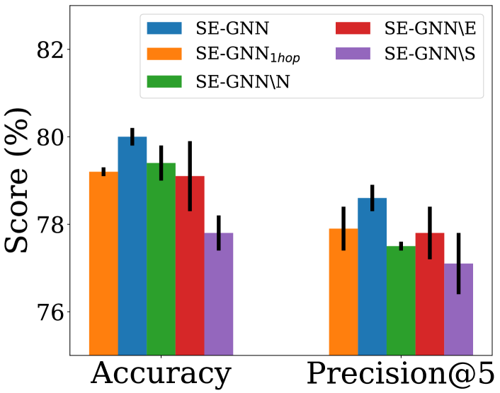
(a) Pubmed

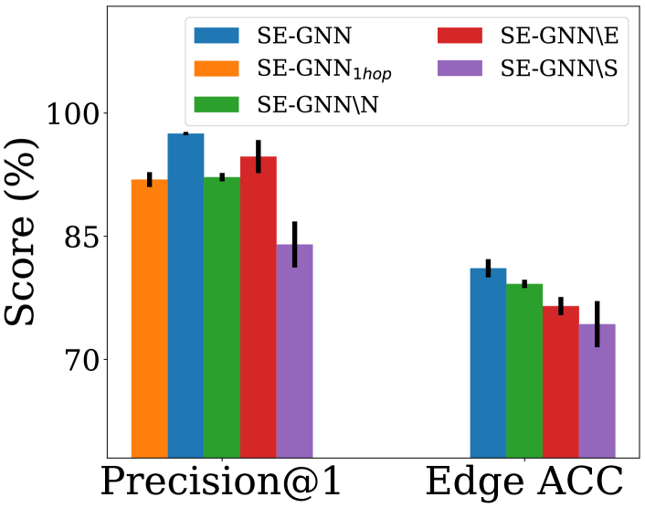
(b) Syn-Cora

Figure 6. Comparisons with SE-GNN and its variants.

5.5. Ablation Study

To answer RQ3, we conduct ablation study to explore the effects of local structure similarity modeling and self-supervision for explanations. SE-GNN utilizes 2-hop local graphs to obtain local structure similarity. To investigate how the similarity modeling will be influenced by the hop of local graphs, we train a variant SE-GNN_1hop which calculates local structure similarity based on 1-hop local graph. To demonstrate the effectiveness of self-supervision on node similarity, we set $\alpha$ in objective function Eq.(14) as 0 to obtain SE-GNN$\backslash$N. Similarly, we remove the self-supervision on local structure similarity and obtain a variant named as SE-GNN$\backslash$E. We also train a variant SE-GNN$\backslash$S which does not incorporate any self-supervision as the reference. Results on Pubmed and Syn-Cora are presented in Figure 6. Since the edge matching in SE-GNN_1hop only considers 1-hop local graph, Edge ACC on 2-hop local graph is not applicable to SE-GNN_1hop. From the Figure 6, we can observe that: (i) The performance of SE-GNN_1hop is significantly lower than SE-GNN in both prediction and explanation. This indicates the importance of incorporating more rich structure information for similarity modeling; and (ii) SE-GNN outperforms SE-GNN$\backslash$E and SE-GNN$\backslash$N by a large margin, which implies that the self-supervision on node similarity and local structure similarity is helpful for identifying interpretable $K$-nearest labeled nodes.

5.6. Parameter Sensitivity Analysis

In this subsection, we investigate how the hyperparameter $\alpha$ and $\beta$ affect the performance of SE-GNN, where $\alpha$ and $\beta$ control the contribution of self-supervision in node similarity modeling and local structure similarity modeling, respectively. We vary $\alpha$ and $\beta$ as $\{0.0001,0.001,0.01,0.11\}$. We report the classification accuracy and precision@5 of $K$-nearest labeled nodes on Pubmed to show the effects of $\alpha$ and $\beta$ on predictions and explanations, respectively. The results are shown in Fig. 7. We find that: (i) with the increase of $\alpha$, the performance in prediction and explanation will first increase and then decrease. When $\alpha$ is too small, little self-supervision is received for node similarity modeling. Low-quality $K$-nearest labeled nodes are obtained, which results in poor performance in classification and explanation. When $\alpha$ is too large, the overall loss function will be dominated by node similarity modeling, which can also lead to a poor overall similarity metric. When $\alpha$ is between 0.001 to 0.01, the performance of SE-GNN in prediction and explanation is generally good. (ii) Similarly, with the increasing of $\beta$, the performance of SE-GNN tends to first increase then decrease. For $\beta$, a value between 0.001 to 0.01 generally gives good performance.

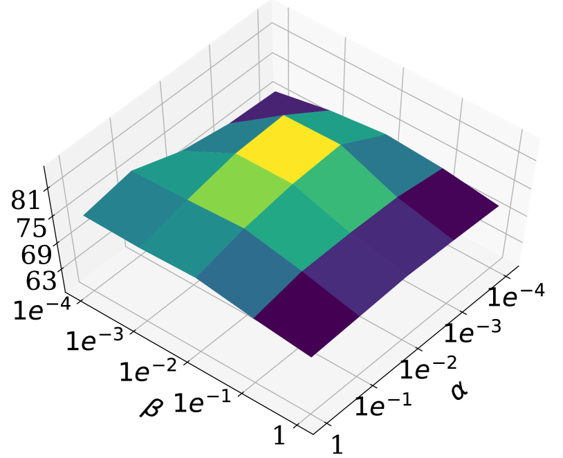
(a) Accuracy (%)

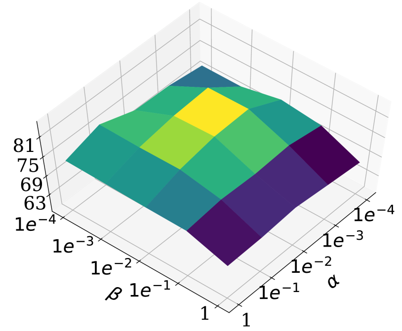
(b) Precision@5 (%)

Figure 7. Parameter sensitive analysis on Pubmed.

6. Conclusion and Future Work

In this paper, we study a novel problem of self-explainable GNNs by exploring $K$-nearest labeled nodes. We propose a new framework, which designs intepretable similarity module for finding $K$-nearest labeled nodes and simultaneously utilizes these nodes for label prediction and explanations. SE-GNN also adopts the contrastive learning to benefit the similarity module. Extensive experiments on real-world and synthetic datasets demonstrate the effectiveness of the proposed SE-GNN for explainable node classification. Ablation study and parameter sensitive analysis are also conducted to understand the contribution of the modules and sensitivity to the hyperparameters. There are several interesting directions which need further investigation. For example, one direction is to extend SE-GNN for explainable link prediction. Another direction is to investigate other pre-text tasks such as using structural identity (Ribeiro et al., 2017) as a self-supervision to help the similarity module.

7. Acknowledgements

This material is based upon work supported by, or in part by, the National Science Foundation (NSF) under grant #IIS1955851, and Army Research Office (ARO) under grant #W911NF-21-1-0198. The findings and conclusions in this paper do not necessarily reflect the view of the funding agency.

References

- (1)
- Alvarez-Melis and Jaakkola (2018) David Alvarez-Melis and Tommi S Jaakkola. 2018. Towards robust interpretability with self-explaining neural networks. arXiv preprint arXiv:1806.07538 (2018).
- Bongini et al. (2021) Pietro Bongini, Monica Bianchini, and Franco Scarselli. 2021. Molecular generative Graph Neural Networks for Drug Discovery. Neurocomputing 450 (2021), 242–252.
- Bruna et al. (2014) Joan Bruna, Wojciech Zaremba, Arthur Szlam, and Yann LeCun. 2014. Spectral networks and locally connected networks on graphs. ICLR (2014).
- Chen et al. (2018) Jie Chen, Tengfei Ma, and Cao Xiao. 2018. Fastgcn: fast learning with graph convolutional networks via importance sampling. ICLR (2018).
- Chen et al. (2020) Ming Chen, Zhewei Wei, Zengfeng Huang, Bolin Ding, and Yaliang Li. 2020. Simple and deep graph convolutional networks. In ICML. PMLR, 1725–1735.
- Chiang et al. (2019) Wei-Lin Chiang, Xuanqing Liu, Si Si, Yang Li, Samy Bengio, and Cho-Jui Hsieh. 2019. Cluster-GCN: An efficient algorithm for training deep and large graph convolutional networks. In SIGKDD. 257–266.
- Dai et al. (2021) Enyan Dai, Charu Aggarwal, and Suhang Wang. 2021. NRGNN: Learning a Label Noise-Resistant Graph Neural Network on Sparsely and Noisily Labeled Graphs. arXiv preprint arXiv:2106.04714 (2021).
- Dai and Wang (2021) Enyan Dai and Suhang Wang. 2021. Say No to the Discrimination: Learning Fair Graph Neural Networks with Limited Sensitive Attribute Information. In WSDM. 680–688.
- Defferrard et al. (2016) Michaël Defferrard, Xavier Bresson, and Pierre Vandergheynst. 2016. Convolutional neural networks on graphs with fast localized spectral filtering. In NeurIPS. 3844–3852.
- Du et al. (2018) Mengnan Du, Ninghao Liu, Qingquan Song, and Xia Hu. 2018. Towards explanation of dnn-based prediction with guided feature inversion. In Proceedings of the 24th ACM SIGKDD International Conference on Knowledge Discovery & Data Mining. 1358–1367.
- Glorot and Bengio (2010) Xavier Glorot and Yoshua Bengio. 2010. Understanding the difficulty of training deep feedforward neural networks. In AISTATS. 249–256.
- Hamilton et al. (2017) Will Hamilton, Zhitao Ying, and Jure Leskovec. 2017. Inductive representation learning on large graphs. In NeurIPS. 1024–1034.
- Hind et al. (2019) Michael Hind, Dennis Wei, Murray Campbell, Noel CF Codella, Amit Dhurandhar, Aleksandra Mojsilović, Karthikeyan Natesan Ramamurthy, and Kush R Varshney. 2019. TED: Teaching AI to explain its decisions. In Proceedings of the 2019 AAAI/ACM Conference on AI, Ethics, and Society. 123–129.
- Huang et al. (2020) Qiang Huang, Makoto Yamada, Yuan Tian, Dinesh Singh, Dawei Yin, and Yi Chang. 2020. Graphlime: Local interpretable model explanations for graph neural networks. arXiv preprint arXiv:2001.06216 (2020).
- Jin et al. (2020a) Wei Jin, Tyler Derr, Haochen Liu, Yiqi Wang, Suhang Wang, Zitao Liu, and Jiliang Tang. 2020a. Self-supervised learning on graphs: Deep insights and new direction. arXiv preprint arXiv:2006.10141 (2020).
- Jin et al. (2020b) Wei Jin, Yao Ma, Xiaorui Liu, Xianfeng Tang, Suhang Wang, and Jiliang Tang. 2020b. Graph structure learning for robust graph neural networks. In SIGKDD. 66–74.
- Kim and Oh (2021) Dongkwan Kim and Alice Oh. 2021. How to find your friendly neighborhood: Graph attention design with self-supervision. In International Conference on Learning Representations.
- Kipf and Welling (2016) Thomas N Kipf and Max Welling. 2016. Semi-supervised classification with graph convolutional networks. arXiv preprint arXiv:1609.02907 (2016).
- Koh and Liang (2017) Pang Wei Koh and Percy Liang. 2017. Understanding black-box predictions via influence functions. In International Conference on Machine Learning. PMLR, 1885–1894.
- Levie et al. (2018) Ron Levie, Federico Monti, Xavier Bresson, and Michael M Bronstein. 2018. Cayleynets: Graph convolutional neural networks with complex rational spectral filters. IEEE Transactions on Signal Processing 67, 1 (2018), 97–109.
- Li et al. (2018) Qimai Li, Zhichao Han, and Xiao-Ming Wu. 2018. Deeper insights into graph convolutional networks for semi-supervised learning. AAAI (2018).
- Luo et al. (2020) Dongsheng Luo, Wei Cheng, Dongkuan Xu, Wenchao Yu, Bo Zong, Haifeng Chen, and Xiang Zhang. 2020. Parameterized Explainer for Graph Neural Network. Advances in Neural Information Processing Systems 33 (2020).
- Mikolov et al. (2013) Tomas Mikolov, Ilya Sutskever, Kai Chen, Greg S Corrado, and Jeff Dean. 2013. Distributed representations of words and phrases and their compositionality. In NeurIPS. 3111–3119.
- Niepert et al. (2016) Mathias Niepert, Mohamed Ahmed, and Konstantin Kutzkov. 2016. Learning convolutional neural networks for graphs. In ICML. 2014–2023.
- Oord et al. (2018) Aaron van den Oord, Yazhe Li, and Oriol Vinyals. 2018. Representation learning with contrastive predictive coding. arXiv preprint arXiv:1807.03748 (2018).
- Papernot and McDaniel (2018) Nicolas Papernot and Patrick McDaniel. 2018. Deep k-nearest neighbors: Towards confident, interpretable and robust deep learning. arXiv preprint arXiv:1803.04765 (2018).
- Plötz and Roth (2018) Tobias Plötz and Stefan Roth. 2018. Neural nearest neighbors networks. Advances in Neural Information Processing Systems 31 (2018), 1087–1098.
- Qiu et al. (2020) Jiezhong Qiu, Qibin Chen, Yuxiao Dong, Jing Zhang, Hongxia Yang, Ming Ding, Kuansan Wang, and Jie Tang. 2020. Gcc: Graph contrastive coding for graph neural network pre-training. In Proceedings of the 26th ACM SIGKDD International Conference on Knowledge Discovery & Data Mining. 1150–1160.
- Ren et al. (2014) Weiqiang Ren, Yinan Yu, Junge Zhang, and Kaiqi Huang. 2014. Learning convolutional nonlinear features for k nearest neighbor image classification. In 2014 22nd international conference on pattern recognition. IEEE, 4358–4363.
- Ribeiro et al. (2017) Leonardo FR Ribeiro, Pedro HP Saverese, and Daniel R Figueiredo. 2017. struc2vec: Learning node representations from structural identity. In Proceedings of the 23rd ACM SIGKDD international conference on knowledge discovery and data mining. 385–394.
- Ribeiro et al. (2016) Marco Tulio Ribeiro, Sameer Singh, and Carlos Guestrin. 2016. ” Why should i trust you?” Explaining the predictions of any classifier. In Proceedings of the 22nd ACM SIGKDD international conference on knowledge discovery and data mining. 1135–1144.
- Selvaraju et al. (2017) Ramprasaath R Selvaraju, Michael Cogswell, Abhishek Das, Ramakrishna Vedantam, Devi Parikh, and Dhruv Batra. 2017. Grad-cam: Visual explanations from deep networks via gradient-based localization. In Proceedings of the IEEE international conference on computer vision. 618–626.
- Sen et al. (2008) Prithviraj Sen, Galileo Namata, Mustafa Bilgic, Lise Getoor, Brian Galligher, and Tina Eliassi-Rad. 2008. Collective classification in network data. AI magazine 29, 3 (2008), 93–93.
- Shrikumar et al. (2017) Avanti Shrikumar, Peyton Greenside, and Anshul Kundaje. 2017. Learning important features through propagating activation differences. In International Conference on Machine Learning. PMLR, 3145–3153.
- Shu et al. (2019) Kai Shu, Limeng Cui, Suhang Wang, Dongwon Lee, and Huan Liu. 2019. defend: Explainable fake news detection. In Proceedings of the 25th ACM SIGKDD International Conference on Knowledge Discovery & Data Mining. 395–405.
- Sun et al. (2019) Fan-Yun Sun, Jordan Hoffmann, Vikas Verma, and Jian Tang. 2019. Infograph: Unsupervised and semi-supervised graph-level representation learning via mutual information maximization. arXiv preprint arXiv:1908.01000 (2019).
- Sun et al. (2020) Ke Sun, Zhanxing Zhu, and Zhouchen Lin. 2020. Multi-stage self-supervised learning for graph convolutional networks. AAAI (2020).
- Tang et al. (2020) Xianfeng Tang, Yandong Li, Yiwei Sun, Huaxiu Yao, Prasenjit Mitra, and Suhang Wang. 2020. Transferring Robustness for Graph Neural Network Against Poisoning Attacks. In WSDM. 600–608.
- Veličković et al. (2018a) Petar Veličković, Guillem Cucurull, Arantxa Casanova, Adriana Romero, Pietro Lio, and Yoshua Bengio. 2018a. Graph attention networks. ICLR (2018).
- Veličković et al. (2018b) Petar Veličković, William Fedus, William L Hamilton, Pietro Liò, Yoshua Bengio, and R Devon Hjelm. 2018b. Deep graph infomax. arXiv preprint arXiv:1809.10341 (2018).
- Wang et al. (2019a) Daixin Wang, Jianbin Lin, Peng Cui, Quanhui Jia, Zhen Wang, Yanming Fang, Quan Yu, Jun Zhou, Shuang Yang, and Yuan Qi. 2019a. A Semi-supervised Graph Attentive Network for Financial Fraud Detection. In ICDM. IEEE, 598–607.
- Wang et al. (2019b) Hongwei Wang, Fuzheng Zhang, Mengdi Zhang, Jure Leskovec, Miao Zhao, Wenjie Li, and Zhongyuan Wang. 2019b. Knowledge-aware graph neural networks with label smoothness regularization for recommender systems. In SIGKDD. 968–977.
- Wu et al. (2020) Zonghan Wu, Shirui Pan, Fengwen Chen, Guodong Long, Chengqi Zhang, and S Yu Philip. 2020. A comprehensive survey on graph neural networks. IEEE transactions on neural networks and learning systems (2020).
- Xu et al. (2018) Keyulu Xu, Weihua Hu, Jure Leskovec, and Stefanie Jegelka. 2018. How powerful are graph neural networks? arXiv preprint arXiv:1810.00826 (2018).
- Ying et al. (2019) Zhitao Ying, Dylan Bourgeois, Jiaxuan You, Marinka Zitnik, and Jure Leskovec. 2019. Gnnexplainer: Generating explanations for graph neural networks. In Advances in neural information processing systems. 9244–9255.
- You et al. (2020) Yuning You, Tianlong Chen, Yongduo Sui, Ting Chen, Zhangyang Wang, and Yang Shen. 2020. Graph contrastive learning with augmentations. Advances in Neural Information Processing Systems 33 (2020).
- Yuan et al. (2019) Hao Yuan, Yongjun Chen, Xia Hu, and Shuiwang Ji. 2019. Interpreting deep models for text analysis via optimization and regularization methods. In Proceedings of the AAAI Conference on Artificial Intelligence, Vol. 33. 5717–5724.
- Yuan et al. (2020) Hao Yuan, Jiliang Tang, Xia Hu, and Shuiwang Ji. 2020. Xgnn: Towards model-level explanations of graph neural networks. In Proceedings of the 26th ACM SIGKDD International Conference on Knowledge Discovery & Data Mining. 430–438.
- Zeiler and Fergus (2014) Matthew D Zeiler and Rob Fergus. 2014. Visualizing and understanding convolutional networks. In European conference on computer vision. Springer, 818–833.
- Zhao et al. (2020) Tianxiang Zhao, Xianfeng Tang, Xiang Zhang, and Suhang Wang. 2020. Semi-Supervised Graph-to-Graph Translation. In CIKM. 1863–1872.
- Zhao et al. (2021) Tianxiang Zhao, Xiang Zhang, and Suhang Wang. 2021. GraphSMOTE: Imbalanced Node Classification on Graphs with Graph Neural Networks. In WSDM. 833–841.
- Zhu et al. (2020) Qikui Zhu, Bo Du, and Pingkun Yan. 2020. Self-supervised Training of Graph Convolutional Networks. arXiv preprint arXiv:2006.02380 (2020).
- Zügner et al. (2018) Daniel Zügner, Amir Akbarnejad, and Stephan Günnemann. 2018. Adversarial attacks on neural networks for graph data. In SIGKDD. 2847–2856.
- Zügner and Günnemann (2019) Daniel Zügner and Stephan Günnemann. 2019. Adversarial attacks on graph neural networks via meta learning. arXiv preprint arXiv:1902.08412 (2019).