Deep Reinforcement Learning for Dynamic Band Switch in Cellular-Connected UAV
Abstract
The choice of the transmitting frequency to provide cellular-connected Unmanned Aerial Vehicle (UAV) reliable connectivity and mobility support introduce several challenges. Conventional sub-6 GHz networks are optimized for ground Users (UEs). Operating at the millimeter Wave (mmWave) band would provide high-capacity but highly intermittent links. To reach the destination while minimizing a weighted function of traveling time and number of radio failures, we propose in this paper a UAV joint trajectory and band switch approach. By leveraging Double Deep Q-Learning we develop two different approaches to learn a trajectory besides managing the band switch. A first blind approach switches the band along the trajectory anytime the UAV-UE throughput is below a predefined threshold. In addition, we propose a smart approach for simultaneous learning-based path planning of UAV and band switch. The two approaches are compared with an optimal band switch strategy in terms of radio failure and band switches for different thresholds. Results reveal that the smart approach is able in a high threshold regime to reduce the number of radio failures and band switches while reaching the desired destination.
Index Terms:
UAV, UE, trajectory, Deep Reinforcement Learning, cellular network, sub-6 GHz, mmWave- 3G
- Third Generation
- 4G
- Fourth Generation
- 5G
- Fifth Generation
- 6G
- Sixth Generation
- 3GPP
- 3rd Generation Partnership Project
- BB
- Base Band
- BBU
- Base Band Unit
- BER
- Bit Error Rate
- BH
- Backhaul
- BPP
- Binomial Point Process
- BS
- Base Station
- BW
- bandwidth
- C-RAN
- Cloud Radio Access Networks
- CAPEX
- Capital Expenditure
- CDF
- Cumulative Distribution Function
- CoMP
- Coordinated Multipoint
- CPRI
- Common Public Radio Interface
- CU
- Centralized Unit
- D2D
- Device-to-Device
- DAC
- Digital-to-Analog Converter
- DAS
- Distributed Antenna Systems
- DBA
- Dynamic Bandwidth Allocation
- DDQN
- Double Deep Q-Learning
- DL
- Downlink
- DNN
- Deep Neural Network
- DQN
- Deep Q-Network
- DDQN
- Double DQN
- DU
- Distributed Unit
- FBMC
- Filterbank Multicarrier
- FEC
- Forward Error Correction
- FH
- Fronthaul
- FL
- Federated Learning
- FFR
- Fractional Frequency Reuse
- FSO
- Free Space Optics
- GS
- Ground Station
- GSM
- Global System for Mobile Communications
- HAP
- High Altitude Platform
- HetNet
- Heterogeneous Network
- HL
- Higher Layer
- HARQ
- Hybrid-Automatic Repeat Request
- KPI
- Key Performance Indicator
- kg
- Kilogramm
- IoT
- Internet of Things
- LAN
- Local Area Network
- LAP
- Low Altitude Platform
- LL
- Lower Layer
- LoS
- Line of Sight
- LTE
- Long Term Evolution
- LTE-A
- Long Term Evolution Advanced
- MAC
- Medium Access Control
- MAP
- Medium Altitude Platform
- MC
- Monte Carlo
- MDP
- Markov Decision Process
- ML
- Medium Layer
- MME
- Mobility Management Entity
- mmWave
- millimeter Wave
- MIMO
- Multiple Input Multiple Output
- ML
- Machine Learning
- MSE
- Mean Square Error
- NFP
- Network Flying Platform
- NFPs
- Network Flying Platforms
- NN
- Neural Network
- NLoS
- Non-Line of Sight
- RL
- Reinforcement Learning
- NR
- New Radio
- OFDM
- Orthogonal Frequency Division Multiplexing
- PAM
- Pulse Amplitude Modulation
- PAPR
- Peak-to-Average Power Ratio
- Probability Density Function
- PER
- Prioritized Experience Replay
- PGW
- Packet Gateway
- PHY
- physical layer
- PP
- Poisson Process
- PSO
- Particle Swarm Optimization
- PTP
- Poin to Point
- QAM
- Quadrature Amplitude Modulation
- QoE
- Quality of Experience
- QoS
- Quality of Service
- QPSK
- Quadrature Phase Shift Keying
- RAU
- Remote Access Unit
- RAN
- Radio Access Network
- RB
- Resource Block
- RF
- Radio Frequency
- RN
- Remote Node
- RRH
- Remote Radio Head
- RRU
- Remote Radio Unit
- RRC
- Radio Resource Control
- RRU
- Remote Radio Unit
- RSS
- Received Signal Strength
- RSRP
- Reference Signals Received Power
- RU
- Remote Unit
- SCBS
- Small Cell Base Station
- SDN
- Software Defined Network
- SINR
- Signal-to-Noise-plus-Interference Ratio
- SIR
- Signal-to-Interference Ratio
- SNR
- Signal-to-Noise Ratio
- SON
- Self-organising Network
- TETRA
- Trans-European Trunked Radio
- TD
- Temporal Difference
- TDD
- Time Division Duplex
- TD-LTE
- Time Division LTE
- TDM
- Time Division Multiplexing
- TDMA
- Time Division Multiple Access
- UE
- User Equipment
- UL
- Uplink
- UAV
- Unmanned Aerial Vehicle
- UPA
- Uniform Planar Square Array
I Introduction
Integrating Unmanned Aerial Vehicles into cellular communication systems as User Equipments is envisioned as an effective solution to support the UAV’s mission specific rate-demanding data communication while improving the robustness of the UAV navigation [1]. This vision of cellular connected UAVs communication, however, poses new research challenges due to the significant differences from conventional communication systems. UAVs-UE have typically higher altitude, higher mobility and have more stringent constraints on the power and operational time than the corresponding ground ones [2]. In addition, the existing cellular network operating at sub-6 GHz is bandwidth limited and perform poorly at high UAV heights, due to the interference perceived from the down-tilted antennas at the ground Base Stations [3]. As a consequence, during its trajectory, a UAV is very likely to experience radio link failures. The UAVs’ mobility and flexibility offer a degree of freedom to circumvent these issues. The UAV path design that aims to respect a quality-of-connectivity constraint and minimize the travelling time goes under the name of Communication-aware trajectory. Several works have optimized the UAV trajectory under connectivity constraints using graph based [4] or dynamic programming based solutions [5]. The above traditional optimization solutions are time consuming and computationally complex. For this reason, Reinforcement Learning (RL) approaches have been recently investigated. Compared to a traditional optimization approach, RL is able of making decisions interacting iteratively with the environment. A double Q-Learning approach is proposed in [6] to solve a joint trajectory and outage time constraint problem. A Temporal Difference (TD) learning method is utilized in [7] to design the UAV-UE trajectory while minimizing the mission completion time and the disconnection duration.
Besides, exploiting their mobility, UAVs can establish short Line of Sight (LoS) communication links, that represents an ideal situation to transmit at millimeter Wave (mmWave) band. A mmWave link offers a wide spectrum and enables the use of directional beamforming, providing high data rate [8]. The work in [8] addresses the cellular connected UAV communication-aware trajectory problem learning simultaneously the mmWave beam and trajectory via Deep Q-Network (DQN) to improve the Uplink (UL) performance. However, due to the severe attenuation and sensitivity to blockages, mmWave links are highly intermittent, leading to frequent radio failures at low UAV altitudes [9].
A promising solution to improve the system robustness is to support two different frequency ranges, leading to integrated dual mode sub-6 GHz/mmWave systems [10]. Dual connectivity would allow to exploit the complementary advantages of both the frequency bands and reduce consistently outage status through band switch algorithms. Some literature has recently studied the band switch problem for conventional ground UEs in a 2D environment. Works in [11]-[12] propose Machine Learning (ML) classifiers that select the best band based on previous rate measurements within a temporal window. Within the UAV communication context, in [13] UAVs are equipped with dual band mmWave and sub-6 GHz communication modules to act as relays to minimize the total service time, but the switch algorithm between the bands is not investigated.
In this paper, differently from previous works, we aim to solve the communication aware 3D trajectory problem of UAV-UE proposing a learning strategy to both manage the trajectory and the band switch policy. We firstly formulate a trajectory problem in order to minimize the travelling time and radio failures of the UAV. Then we propose a 3D DQN based algorithm to dynamically solve it adjusting the position and the operating frequency of the UAV-UE. Finally, we present also a blind switch strategy and introduce a baseline optimal band switch policy. We compare the performance of these three approaches in term of number of radio failures and band switches in the result section. We observe that the smart approach significantly improves the performance of the ground BS link for stringent thresholds.
II System Model
II-A Network Topology
Consider the downlink of a dual band wireless cellular network, that operates in two frequency bands with frequency and bandwidth , . A set of ground Distributed Units is deployed in an area , connected to a single Centralized Unit (CU), and serve a set of UAV-UEs. Both DUs and UEs are equipped with interfaces which allow them to transmit at both frequency bands. We assume the transmission occurs in a single frequency at a time, generating inter-cell interference to neighboring cells working at the same frequency band. Each DU is assumed to have Resource Blocks and transmits with same power . Without loss of generality, we focus on a single link to a UAV-UE (hereafter addressed as UAV).
II-B Ground-to-Air Channel Model
In this section we present the path loss, antenna and fading models, considering a lower sub-6 GHz band and the mmWave band.
II-B1 Path Loss and Antenna Model
The ground-to-air channel model is subject to LoS/ Non-Line of Sight (NLoS) variations based on the building distribution in and UAV height that lead to blockages. For modeling the path loss at sub-6 GHz we consider the urban Macro (UMa) path loss specified in 3rd Generation Partnership Project (3GPP) [14]. The path loss at mmWave follows a path loss model [9]:
| (1) |
where is the ground BS-UAV distance, parameters , and , represent, respectively, the path loss exponent for LoS/NLoS and the path loss at 1 meter distance. Each DU has three sectors separated by as characterized by 3GPP specification [14]. Each sector is equipped with a vertical -element uniform linear array (ULA) at and a Uniform Planar Array (UPA) at tilted with angle and . We denote the total ground DU directional radiation pattern as , where , are elevation and azimuth angles. We assume the UAV is equipped with a conventional omni-directional antenna of unitary gain in any direction to maintain low complexity and cost at the UAV.
II-B2 Fading Model
We model the small scale fading fading power with as a Nakagami-m fading model, that covers a wide range of fading environments, including both sub-6 GHz () and mmWave (). Accordingly, follows a Gamma distribution with .
II-C UAV Mobility Model
The UAV moves at constant speed along a 3D trajectory of duration that can be divided into discrete segments with interval , . is chosen arbitrarily small so that within each step the large scale signal power received by the UAV remains approximately unchanged. Each segment is thus described by its discrete coordinates . The trajectory of the UAV starts from a random position in the given area of interest , delimited by borders while the altitude of the UAV must satisfy , where represents the lower bound of UAVs’ altitude to avoid collisions and represents the upper bound. The trajectory ends when the UAV reaches a final destination .
II-D Communication Model
The achievable rate at in band can be expressed as: where is the bandwidth assigned to the link and the Signal-to-Noise-plus-Interference Ratio (SINR). At each trajectory step , the UAV associates with the m-th DU at position providing the highest average Reference Signals Received Power (RSRP) at the current frequency. Assuming that the associated cell remains unchanged within each trajectory step, the SINR at the UAV can be denoted as:
| (2) |
where is the received power and terms in the denominator are, respectively, the spectral noise and the interference. Note that a subscript to emphasize the dependence of and has been omitted to lighten the notation.
To maintain a reliable connection, DU-UAV link must satisfy a rate threshold . We define a radio failure on the link if occurs at step . In addition, we introduce a failure indicator as:
| (3) |
To avoid a radio failure, at each discrete step the UAV may require the CU a band switch to change the transmission frequency. Prior to formulating the problem, in what follows we introduce the band switch procedure and signalling.
II-E Band switch procedure
The band switch policy industry standard for a conventional ground UE is composed of several iterative steps which can be summarized as follows : 1) if the serving rate at current frequency drops below threshold , the UE initiates a band switch procedure with the serving cell, 2) the UE utilizes a time to measure if a cell at target frequency offers a higher RSRP than the serving cell, 4) if yes, the UE triggers a band switch procedure and reports the measurement back to the DU, 5) the CU makes a decision on the suitable DU at target frequency for band switch, based on the UE measurements. Applying the above policy to UAV communications would introduce several challenges. The mobility of the UAV might cause deep RSRP fluctuations between two consequent trajectory steps and . This might lead to subsequent band switch procedures and potential ping-pong effect. Note that, due to the measurement gap, in case of several band switches the effective throughput at the UE suffers a significant reduction [12]. Thus, we modify the above band switch procedure to adapt it for a UAV moving between cells belonging to different DUs controlled by a central CU. Here, motivated by the above mentioned challenges, we formulate a real-time trajectory and band switch procedure exploiting the capabilities of a RL based policy. In the next sections we formulate the problem and propose two DQN algorithms for joint UAV-UE trajectory and band switch.
II-F Problem formulation
The goal of the UAV is to reach the destination in the minimum amount of steps while minimizing the number of radio failures. At the same time, to avoid a radio failure and meet the quality of service requirement, at the beginning of each discrete step , the operating frequency can be switched between and . Denoting as the trajectory steps, the number of band switches, the above problem can be mathematically formulated as:
| (4a) | ||||
| s.t. | (4b) | |||
| (4c) | ||||
where weight the summation of the arguments, (4b), (4c) are the starting and final positions. Problem (4) cannot be readily handled by conventional optimization methods due to the non trivial design of , function for each position of the fading, and the antenna model described in Section II.
III Band Switching as a Deep Reinforcement Learning Problem
In the standard RL setting an agent acts in an environment over discrete time steps. Given that problem (4) has been formulated in a discrete form, we can directly map it into a Markov Decision Process (MDP) 5-tuple , with space state , action space , state transition probability , reward function , and discount factor . At each time step , the agent receives an observation and selects an action , receives reward from the environment and goes from state to a new state where the cycle restart. We assume an episodic setup, where an episode starts with time step and concludes with time step . Here the states consist in the 3D location of the UAV and band switch indicator , such as . Both the location and the band switch indicator are the input of the neural network. The agent, placed at the CU to overcome the limited onboard computing capacity, selects an action in a set of actions in the action space . The action can be represented by parameters where corresponds to the movements of the UAV in altitude (up or down) or in the horizontal direction (left-right-forward-back). In addition, if is positive, the CU triggers a band switch in the network operating frequency without a measurement gap. Based on the selected action the UAV moves in the desired direction for a distance at speed reaching the position . Our goal is to predict the UAV direction along with the transmitting frequency to avoid radio failures and reach the destination using the current rate measurement. With this aim we define as reward function as: is a negative cost and forces the UAV to reach the destination in the minimum amount of steps. denotes the cost for entering in low normalized rate regions (), that lead to radio failures. accounts for the band switches occurred until time step . Note that is a cost since a high number of band switches is not desirable. Thus, , , balance the impact of the three factors on the reward function and need to be properly adjusted.
In order to achieve the desired goal, we need to find a policy that maximizes the long-term average of both connectivity and path guidance. We recall that a policy is defined as the probability of taking action in state , through interacting with the environment. Based on this, the problem is equivalent to find a policy that maximizes a cumulative discounted reward over the long run:
| (5) |
The discount factor in (5) regulates the relative importance of future and immediate rewards.
III-A DDQN for UAV-UE Trajectory and Smart Band Switch
In the convention RL approach, for a given policy , a state-action function is introduced to represent the expected return after taking action in state . In order to deal with large state/action space dimensions DQN was introduced in [15] to approximate the optimal Q-function using a Deep Neural Network (DNN) such that where are the network’ weights. The transitions , with are stored into a memory of finite capacity size and randomly picked when performing a Q-value update. At each iteration, DQN is trained to minimize the loss:
| (6) |
where is the target function given by , where is introduced following the target network mechanism. We denote the primary DNN network weight matrix and target DNN weight matrix as and . We consider a fully connected DNN for both networks and the DNN parameters are updated with the parameters every fixed number of steps to improve the convergence of the algorithm. Among the improvements and extensions of the baseline DQN algorithm, we implement Double DQN (DDQN) which reduces the overstimation bias of DQN with a simple modification of the update rule. In particular, the target function becomes:
| (7) |
In Algorithm (1) we introduce the complete pseudocode.
III-A1 Analysis of the Smart Switch Algorithm
The proposed algorithm aims to solve the challenges of the state of the art band switch policy presented in Section II-E. After the initialization procedures, the agent performs an initial exploration of the state space through an -greedy policy (lines () in Algorithm (1)). The UAV moves in a custom environment consisting of the area under consideration covered by the dual band network, the possible UAV locations and discrete action space. At each episode, the environment resets the source UAV location, computes new observations and rewards based on the desired action until it reaches destination. Since the band switch indicator is included as input state of the DNN, goal of the agent is to learn by experience in which states bandswitching is beneficial, without the need for measurement of gaps.
Next, we introduce a Blind DQN Algorithm for the joint UAV-UE Trajectory and Band Switch and an Optimal Algorithm.
III-B DDQN for joint UAV-UE Trajectory and Blind Band Switch
To solve the optimization problem (4) we propose also a Blind algorithm, that focuses on learning the best trajectory to reach the destination and switches the transmitting frequency any time a radio failure occurs. Differently from the Algorithm presented in Section III-A, the states consist of the 3D location of the UAV and the action in the direction only. In addition, in the reward function, . The Algorithm pseudocode is omitted here since it is similar to the one presented in Algorithm 1. This band switch algorithm without information about the instantaneous rate at both frequencies, cannot guarantee that the throughput after the band switch will be higher than the original one.
III-C Optimal DDQN for UAV-UE Trajectory
Finally, as benchmark, we introduce an Optimal Algorithm. At each trajectory step the agent knows the instantaneous achievable rate of the two different bands. Therefore, the CU at each step coordinates the DUs to transmit at the best frequency, minimizing the radio failures due to a wrong choice about the band.
IV Simulation Results
In this section we evaluate the performance of the proposed DQN algorithms and we benchmark them with the Optimal Policy.
| Parameter | Description | Value |
|---|---|---|
| / | UAV Max/Min Height | 120/60 m |
| / | Antenna Element / | 8/64 |
| / | Antenna Tilt / | -10/10 |
| Noise Power / | -204/-120 db/Hz | |
| time step length | 0.5 s | |
| -greedy variable | 0.4 | |
| UAV Max Moves | 200 | |
| discount factor | 1 | |
| Replay Memory Size | 100000 | |
| , , | Rewards weights | 0.1, 0.8, 0.1 |
We consider a deployment of 5 dual band DUs in an area of side km where buildings are modeled as for the ITU-R urban statistical model [16] with maximum height of m. The two frequency bands considered are GHz and kHz, and GHz and = 1800 kHz. We use one RB at sub-6 GHz while ten at mmWave [12]. We choose to transmit at W at mmWave and at W at sub-6 GHz. In the proposed DQN algorithms, the DNN consists of input layer, four hidden layers, one output layer, all fully connected feedforward, activated using Rectified Linear Units (ReLU) and trained with Adam optimizer. Each training run was conducted using a batch size of for a minimum of iterations. Table I presents all simulation parameters.
IV-A Simulation Environment
In Figure 1(a), we show the rate trend along with the same trajectory episode at sub-6 GHz and mmWave.
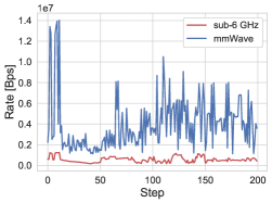
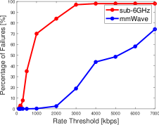
The rate has sudden drops both at sub6GHz and mmWave, due to the presence of fading and obstacles. In particular, at mmWave, the rate can be very high or very low, due to the higher bandwidth and, at the same time, high sensitivity to blockages. In Figure 1(b) we show the total percentage of detachments completing the UAV missions at one frequency only, sub-6 GHz or mmWave band, and without any band switch mechanism. Intuitively, the number of failures increases as we increase the rate threshold. Both the above results motivate the band switching approach presented in this paper.
IV-B Band Switch Policies
The UAV-UE starts its trajectory at sub-6 GHz and can switch to the 28 GHz band. We consider a low threshold of at sub-6 GHz and at mmWave (Treshold 1), a threshold of at sub-6 GHz and at mmWave (Treshold 2) and a high Threshold 3 of at sub-6 GHz and at mmWave. In Figure 2(a) we compare the blind, the smart and optimal switch algorithms for increasing thresholds in term of average percentage of radio failures.
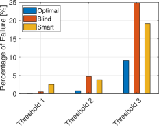
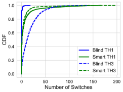
We observe that at low thresholds, the smart approach performs similarly to the blind approach. By increasing the threshold, and as consequence, the probability of a radio failure, we observe a higher increase in the number of radio failures for the blind approach. While the blind approach switches the band anytime a radio failure occurs, the smart one offers the agent a generic framework that, interacting with the environment, learns to minimize the number of radio failures switching the band only when the target frequency provides higher throughput. As confirmation of this, in Figure 2(b) we plot the Cumulative Distribution Function (CDF) of the number of band switches of the blind and smart approach for Threshold 1 and 3. We observe that in a high throughput regime, the smart approach outperforms the blind approach and can significantly reduce the number of switches.
V Conclusion
In this paper, we propose a DQN based approach to solve a communication aware trajectory problem for cellular UAV. In order to minimize the number of radio failures while reaching its target destination, we consider the UAV to exploit band switch policies without prior knowledge of the environment. We define and compare two joint trajectory and band switch DQN algorithms, that differentiate based on how the agent decide to switch the transmitting frequency. We show that a smart switch approach, where the band switch indicator is included as input state of the DNN, is able to outperform a blind approach in a high threshold regime.
Acknowledgment
This work was supported by the Irish Research Council under Grant GOIPG and in part by the Science Foundation Ireland under Grant Numbers RC and /NSFC/.
References
- [1] Y. Zeng, J. Lyu, and R. Zhang, “Cellular-Connected UAV: Potential, Challenges, and Promising Technologies,” IEEE Wireless Commun., vol. 26, no. 1, pp. 120–127, 2018.
- [2] M. Mozaffari et al., “A tutorial on UAVs for wireless networks: Applications, Challenges, and Open Problems,” IEEE commun. surveys & tutorials, vol. 21, no. 3, pp. 2334–2360, 2019.
- [3] G. Geraci et al., “Understanding UAV cellular communications: From existing networks to massive MIMO,” IEEE Access, vol. 6, pp. 67 853–67 865, 2018.
- [4] S. Zhang and R. Zhang, “Trajectory Design for Cellular-Connected UAV under Outage Duration Constraint,” in Proc. IEEE International Conference on Communications (ICC), May 2019.
- [5] E. Bulut and I. Guevenc, “Trajectory Optimization for Cellular-Connected UAVs with Disconnectivity Constraint,” in Proc. IEEE International Conference on Communications (ICC), May 2018.
- [6] B. Khamidehi and E. S. Sousa, “A Double Q-Learning Approach for Navigation of Aerial Vehicles with Connectivity Constraint,” in Proc. IEEE International Conference on Communications (ICC), Jun. 2020.
- [7] Y. Zeng and X. Xu, “Path Design for Cellular-Connected UAV with Reinforcement Learning,” in Proc. IEEE Global Communications Conference (GLOBECOM), Dec. 2019.
- [8] P. Susarla et al., “Learning-Based Trajectory Optimization for 5G mmwave Uplink UAVs,” in Proc. IEEE International Conference on Communications (ICC), Jun. 2020.
- [9] G. Fontanesi, A. Zhu, and H. Ahmadi, “Outage Analysis for Millimeter-Wave Fronthaul Link of UAV-Aided Wireless Networks,” IEEE Access, vol. 8, pp. 111 693–111 706, June 2020.
- [10] O. Semiari et al., “Integrated Millimeter Wave and Sub-6 GHz wireless Networks: A Roadmap for Joint Mobile Broadband and Ultra-Reliable Low-Latency Communications,” IEEE Wireless Commun., vol. 26, no. 2, pp. 109–115, April 2019.
- [11] D. Burghal, R. Wang, and A. F. Molisch, “Deep Learning and Gaussian Process based Band Assignment in Dual Band Systems,” arXiv preprint arXiv:1902.10890, 2019.
- [12] F. B. Mismar et al., “Deep Learning Predictive Band Switching in Wireless Networks,” IEEE Trans. Wireless Commun., Sept. 2020.
- [13] H. Ghazzai et al., “Trajectory Optimization for Cooperative Dual-Band UAV Swarms,” in Proc. IEEE Global Communications Conference (GLOBECOM), Dec. 2018.
- [14] “Technical specification group radio access network; study on enhanced LTE support for aerial vehicles (release 15),” 3GPP, TR 36.777, Dec 2017.
- [15] V. Mnih et al., “Human-Level Control Through Deep Reinforcement Learning,” Nature, vol. 518, no. 7540, pp. 529–533, 2015.
- [16] Propagation Data and Prediction Methods Required for the Design of Terrestrial Broadband Radio Access Systems Operating in a Frequency Range From 3 to 60 GHz, ITU-R Recommendation P.1410-5, 2012.