Price modelling under generalized fractional Brownian motion

Abstract

The Generalized fractional Brownian motion (gfBm) is a stochastic process that acts as a generalization for both fractional, sub-fractional, and standard Brownian motion. Here we study its use as the main driver for price fluctuations, replacing the standard Brownian Brownian motion in the well-known Black-Scholes model. By the derivation of the generalized fractional Ito’s lemma and the related effective Fokker-Planck equation, we discuss its application to both the option pricing problem valuing European options, and the computation of Value-at-Risk and Expected Shortfall. Moreover, the option prices are computed for a CEV-type model driven by gfBm.

Keywords: Fractional Brownian motion; Sub-fractional Brownian motion; Generalized fractional Brownian motion; Option pricing; Econophysics.

This version: March 19, 2024

1 Introduction

The Black-Scholes model [1], in shortly BS, is generally categorized as the cornerstone of financial engineering. By means of Geometric Brownian motion and Delta-hedging arguments, the model provides a valuation formula solving the partial differential equation which rules the vanilla option pricing.

However, some “stylized facts” query the BS assumptions. One of them is the lack of memory (or Markovian property) due to the use of a standard Brownian motion (Bm) in the price fluctuation modeling. One attempt to correct it, is the replacement of the Bm by a fractional Brownian motion (fBm) [2], a Gaussian process characterized by self-similarity, Holder paths, stationary increments, and long (short) range dependence for $H>1/2\,(H<1/2)$. The parameter $H\in(0,1)$ is called the Hurst exponent and for $H=1/2$ reduces the fBm to a Bm. An explicit close-form option price solution for the fractional BS model is given in refs. [3, 4] followed by a lot of research outputs that consider the analytical valuation of financial derivatives with underlying assets driven by fBm. Recent developments include, e.g., the pricing of Asian options [5], the European option pricing under the constant elasticity of variance (CEV) model [6], default risk derivatives as Credit Default Swaps [7] or vulnerable options [8], and the consideration of jumps or Fuzzy theory [9].

Bojdecki et al. [10] introduce a new stochastic process called sub-fractional Brownian motion (sfBm), which retains the most properties of fBm but differs in some key issues related to its non-overlapping increments: non-stationarity and weakly covariance (with higher decay rate). More details about this process are described in [11]. Some applications of sfBm in finance have been published recently. For example, Xu and Zhou [12] addressed the pricing of perpetual American options, Wang and its coauthors [13] studied the pricing of geometric Asian power options, and Ji et al. [14] the barrier option valuation in a jump environment. Outside of the BS environment, we could list, among others, the sub-fractional Poisson volatility model [15], the sub-fractional Vasicek model [16], the sub-fractional CEV [17] which was derived and empirically tested through real option data finding both an improvement with respect to classical CEV and the BS types (under classical, fractional and sub-fractional diffusions), and the capability to capture the option prices temporal structure under different maturities.

Alternatively, Zili [18] proposed a new Gaussian process called generalized fractional Brownian motion (gfBm in shorthand notation), defined as a linear combination of a two-sided fBm, which serves as a generalization for both Bm, fBm, and sfBm. This process is featured with the ability to control the level of correlation between the increments and the ductility to arise stationary and non-stationary increments. A review of its main properties can be found in refs. [18, 19].

This manuscript aims to use the gfBm for financial modelling and its application in the computation of risk-measures and the pricing of European options. The rest of the paper is organized in the following way. First, we describe some helpful properties and auxiliary about gfBm, including the generalized fractional Itô lemma and the related ’effective’ Fokker-Planck equation. Later, in Section 3, we arrive at the transition density function for a price process driven by a gfBm with proportional drift (Black-Scholes type). In Section 4, we derive the Value-at-Risk and Expected Shortfall, in addition to the close-form formula for European vanilla contracts. At next, a CEV-type exension is proposed computing European Call and Put prices. Finally, the main conclussions are displayed.

2 On the Generalized fractional Brownian motion

Let $(a,b)\neq\left(0,0\right)\in\mathbb{R}^{2}$ and $H\in\left(0,1\right)$. Be also $B_{t}^{H}$ a two-sided fBm, $\forall t\in\mathbb{R}_{+}$. Then, the centered Gaussian process $Z_{t}^{H,a,b}$ is called gfBm and defined by:

$$Z_{t}^{H,a,b}=aB_{t}^{H}+bB_{-t}^{H}$$ (1)

Depending on the values of $a,b$, and $H$ we could recover both Bm, fBm, and sfBm. Its clear to see from the above definition that $Z_{t}^{H,a,0}$ reduced the process to a fBm, $Z_{t}^{1/2,a,0}$ matches to a standard Bm, while $Z_{t}^{H,\frac{1}{\sqrt{2}},\frac{1}{\sqrt{2}}}=\left(B_{t}^{H}+B_{-t}^{H}\right)/\sqrt{2}=\xi_{t}^{H}$ corresponds to a definition of sfBm [10, Eq. 2.1].

From Eq. (1) we can also determine the covariance and variance of the process. Let $t,s\geq 0$. Then the following results apply:

$$E\left(Z_{t}^{H,a,b}\cdot Z_{s}^{H,a,b}\right)=\frac{\left(a+b\right)^{2}}{2}\left(s^{2H}+t^{2H}\right)-ab\left(s+t\right)^{2H}-\frac{a^{2}+b^{2}}{2}\left|t-s\right|^{2H}$$

$$E\left[\left(Z_{t}^{H,a,b}\right)^{2}\right]=\left[\left(a+b\right)^{2}-2^{2H}ab\right]t^{2H}$$

From refs. [18, 19], we observe that the above covariance structure has a couple of implications in the study of non-overlapping increments of the process (1). First, the increments are non-stationary unless $b=0$; i.e., in the case of a fBm. Second, they are positively (resp. negative) correlated if $H>1/2$ ($H<1/2$). Moreover, the magnitude of the autocorrelation is stronger, weaker, or in between than the values provided by fBm and sfBm, depending on the selected values of the triple $\left(H,a,b\right)$. Indeed, we will have long-range dependence (slow decay on the autocorrelation) for any $a\neq b$ and $H>1/2$, while for $H<1/2$ or $a=b$ and any $H$, short-range dependence (high decay on the autocorrelation) appears. These features equipped the gfBm with the ability to control the level of correlation between the increments of the studied phenomena and the ductility to arise stationary and non-stationary increments.

On the other hand, since we have a bounded variance, we can derive the related Ito-Wick formula following the approach of Nualart and Taqqu [20]. Let $f=f\left(t,Z_{t}^{H,a,b}\right)\in C^{1,2}\left(\left(0,\infty\right)\times\mathbb{R}\right)$. Then:

$$\text{d}f =\frac{\partial f}{\partial t}\text{d}t+\frac{\partial f}{\partial z}\text{d}Z_{t}^{H,a,b}+\frac{1}{2}\frac{\partial^{2}f}{\partial z^{2}}\text{d}\left\{\left[\left(a+b\right)^{2}-2^{2H}ab\right]t^{2H}\right\}$$

$$=\frac{\partial f}{\partial t}\text{d}t+\frac{\partial f}{\partial z}\text{d}Z_{t}^{H,a,b}+\frac{1}{2}\frac{\partial^{2}f}{\partial z^{2}}\left\{\left[\left(a+b\right)^{2}-2^{2H}ab\right]\text{d}t^{2H}\right\}$$

$$=\left\{\frac{\partial f}{\text{$\partial t$}}+H\left[\left(a+b\right)^{2}-2^{2H}ab\right]t^{2H-1}\frac{\partial^{2}f}{\text{$\partial x^{2}$}}\right\}\text{d}t+\frac{\partial f}{\text{$\partial x$}}\text{d}Z_{t}^{H,a,b}$$ (2)

It’s easy to show that for $a=b=1/\sqrt{2}$, the Eq. (2) corresponds to the sub-fractional Itô’s lemma [21]. While, for $\left(a,b\right)=\left(1,0\right)$, we arrive at the fractional Itô ’s lemma. [22]. The standard Itô calculus is recovered for $\left(a,b,H\right)=\left(1,0,1/2\right)$ or $\left(a,b,H\right)=\left(1/\sqrt{2},1/\sqrt{2},1/2\right)$.

In the same way, the previous result can be adapted to more general processes driven by a gfBm. Let $y_{t}$ a stochastic process described by the following stochastic differential equation (SDE):

$$\text{d}y_{t}=\mu\left(y_{t},t\right)\text{d}t+\sigma\left(y_{t},t\right)\text{d}Z_{t}^{H,a,b}$$ (3)

then, the transformation $g=g\left(y_{t},t\right)\in C^{2}\left(\mathbb{R}\right)$ follows:

$$\text{d}g\left(y_{t},t\right)=\left\{\frac{\partial g}{\text{$\partial t$}}+\left(\frac{\partial f}{\text{$\partial y$}}\right)\mu+H\left[\left(a+b\right)^{2}-2^{2H}ab\right]\sigma^{2}t^{2H-1}\frac{\partial^{2}f}{\text{$\partial y^{2}$}}\right\}\text{d}t+\left(\frac{\partial f}{\text{$\partial y$}}\right)\sigma\text{d}Z_{t}^{H,a,b}$$ (4)

The last statement is also useful to derive the related “effective” Fokker-Planck equation that rules the transition density function for the generic process (3). Following [17, Theorem 2.1], the transition density function $P$ is governed by:

$$\frac{\partial P}{\partial t}=H\left[\left(a+b\right)^{2}-2^{2H}ab\right]t^{2H-1}\frac{\partial^{2}}{\partial y^{2}}\left(\sigma^{2}P\right)-\frac{\partial}{\partial y}\left(\mu P\right)$$ (5)

3 Price modelling

Let $S_{t}$ the price of a given stock. We will assume that it follows the BS model driven by gmfBm. Then, under the real physical measure $\mathbb{P}$, the evolution of the price is ruled by:

$$\text{d}S_{t}=\mu S_{t}\text{d}t+\sigma S_{t}\text{d}Z_{t}^{H,a,b}$$ (6)

being $\mu$ and $\sigma$ constant coefficients and $\text{d}Z_{t}^{H,a,b}$ represents the differential form of the process $Z_{t}^{H,a,b}$ defined at Eq. (1).

Applying the change of variable $x=\ln S-\mu t$ and the related Itô’s calculus (Eq. 4), the new process $x$ obeys the following SDE:

$$\text{d}x=-H\left[\left(a+b\right)^{2}-2^{2H}ab\right]t^{2H-1}\text{d}t+\sigma\text{d}Z_{t}^{H,a,b,c}$$ (7)

From Eq. (5), the evolution of the transition density function obeys the following PDE:

$$\frac{\partial P}{\partial t}=\sigma^{2}\left\{H\left[\left(a+b\right)^{2}-2^{2H}ab\right]t^{2H-1}\right\}\left(\frac{\partial^{2}P}{\partial x^{2}}+\frac{\partial P}{\partial x}\right)$$ (8)

with initial condition $P(x,0)=\delta\left(x-x_{0}\right)$, being $x_{0}$ the knowing value of $x$ at the inception time (which implies that the density is concentrated at that point at the beginning).

By the time substitution

$$\tau=\sigma^{2}\left[\left(a+b\right)^{2}-2^{2H}ab\right]t^{2H}$$

Eq. (8) is transformed into a time-homogeneous convection-diffusion equation:

$$\frac{\partial P}{\partial\tau}=\frac{1}{2}\frac{\partial^{2}P}{\partial x^{2}}+\frac{1}{2}\frac{\partial P}{\partial x}$$

After that, moving to a traveling frame of reference $w=x+\tau/2$, we obtain:

$$\frac{\partial P}{\partial\tau}=\frac{1}{2}\frac{\partial^{2}P}{\partial w^{2}}$$ (9)

Eq. (9) corresponds to an standard diffusion equation with constant diffusion coefficient, with fundamental solution:

$$P(w,\tau)=\frac{1}{\sqrt{2\pi\tau}}\exp\left[-\frac{\left(w-w_{0}\right)^{2}}{2\tau}\right]$$ (10)

where $P\left(w,0\right)=P\left(w_{0}\right)=\delta\left(w_{0}\right)$. This initial condition is given by knowing the state of the asset $S$ at the inception time; i.e., $S\left(t=0\right)=S_{0}=\text{e}^{x_{0}}=\text{e}^{w_{0}}$.

After replacing $w$ and $\tau$ as a function of $x$ and $t$, respectively; we finally obtain:

$$P\left(\left.x,t\right|x_{0},0\right)=\left(2\pi\sigma^{2}\left[\left(a+b\right)^{2}-2^{2H}ab\right]t^{2H}\right)^{-\frac{1}{2}}\\ \times\exp\left[-\frac{\left(x-x_{0}+\frac{1}{2}\sigma^{2}\left[\left(a+b\right)^{2}-2^{2H}ab\right]t^{2H}\right)^{2}}{2\sigma^{2}\left[\left(a+b\right)^{2}-2^{2H}ab\right]t^{2H}}\right]$$ (11)

Moreover, the transition probability density function for the price process (6), at time $T$, is given by:

$$P\left(\left.S_{T},T\right|S_{0},0\right)=\frac{\text{e}^{-\frac{\left(\ln\left(\frac{S_{T}}{S_{0}}\right)+rT+\frac{1}{2}\sigma^{2}\left[\left(a+b\right)^{2}-2^{2H}ab\right]T^{2H}\right)^{2}}{2\sigma^{2}\left[\left(a+b\right)^{2}-2^{2H}ab\right]T^{2H};}}}{S_{T}\sqrt{2\pi\sigma^{2}\left[\left(a+b\right)^{2}-2^{2H}ab\right]T^{2H}}}$$ (12)

From the above equation, we can show that the expected rate of return is $\mu$:

$$\mathbb{E^{P}}\left(S_{T}\right) = \int_{0}^{\infty}S_{T}P\left(S_{T},T\right)\text{d}S_{T}$$ (13)

$$= \int_{0}^{\infty}\text{e}^{x_{T}+\mu T}P\left(x_{T},T\right)\text{d}x_{T}$$

$$= \frac{\text{e}^{x_{0}+\mu T}}{\sqrt{2\pi\sigma^{2}\left[\left(a+b\right)^{2}-2^{2H}ab\right]T^{2H}}}\int_{0}^{\infty}\exp\left[-\frac{\left(x-x_{0}-\frac{1}{2}\sigma^{2}\left[\left(a+b\right)^{2}-2^{2H}ab\right]T^{2H}\right)^{2}}{\sigma^{2}\left[\left(a+b\right)^{2}-2^{2H}ab\right]T^{2H}}\right]\text{d}x_{T}$$

$$= \frac{S_{0}\text{e}^{\mu T}}{\sqrt{2\pi}}\int_{0}^{\infty}\exp\left[-\frac{u^{2}}{2}\right]\text{d}u$$

$$= S_{0}\text{e}^{\mu T}$$

4 Applications

4.1 Risk measures

4.1.1 Value-at-risk

A very popular measure for tail-risk is the well-known Value-at-Risk, VaR in short. It computes the minimum losses of a portfolio, for a given investment horizon, considering a fixed-choose risk level $\alpha$. This level is the quantile in the distribution of the future portfolio. In other words, the $\alpha$-VaR set the probability equal to $\alpha$ for a loss greater than VaR. Typical values for $\alpha$ are 1% and 5%. Thus, setting a portfolio from a long position in the asset $S$ (purchased at the inception time), the $\alpha$-VaR at time $T$ will be $S_{0}\text{e}^{rT}-V$, where $V$ is obtained from:

$$\int_{0}^{V}P\left(S_{T},T\right)\text{d}S_{T}=\alpha$$ (14)

Then, assuming that the price is governed by the process 6, from Eqs. 11-12, we get:

$$\alpha = \int_{0}^{V}P\left(S_{T},T\right)\text{d}S_{T}$$ (15)

$$= \int_{-\infty}^{\ln V-\mu t}P\left(x_{T},T\right)\text{d}x_{T}$$

$$= \frac{1}{\sqrt{2\pi\sigma^{2}\left[\left(a+b\right)^{2}-2^{2H}ab\right]T^{2H}}}\int_{-\infty}^{\ln V-\mu t}\exp\left[-\frac{\left(x-x_{0}-\frac{1}{2}\sigma^{2}\left[\left(a+b\right)^{2}-2^{2H}ab\right]T^{2H}\right)^{2}}{\sigma^{2}\left[\left(a+b\right)^{2}-2^{2H}ab\right]T^{2H}}\right]$$

$$= N\left(-\frac{\ln\left(\frac{S_{0}}{V}\right)+\mu T-\frac{1}{2}\sigma^{2}\left[\left(a+b\right)^{2}-2^{2H}ab\right]T^{2H}}{\sigma\sqrt{\left[\left(a+b\right)^{2}-2^{2H}ab\right]T^{2H}}}\right)$$

$$= N\left(-d_{2}^{a,b,H,V}\right)$$

where $N\left(\cdot\right)$ stands for the standard normal cumulative density, and:

$$d_{2}^{a,b,H,V}=\frac{\ln\left(\frac{S_{0}}{V}\right)+\mu T-\frac{1}{2}\sigma^{2}\left[\left(a+b\right)^{2}-2^{2H}ab\right]T^{2H}}{\sigma\sqrt{\left[\left(a+b\right)^{2}-2^{2H}ab\right]T^{2H}}}$$

Then:

$$V=S_{0}\exp\left[\mu T-\frac{1}{2}\sigma^{2}\left[\left(a+b\right)^{2}-2^{2H}ab\right]T^{2H}+N^{-1}\left(\alpha\right)\sigma\sqrt{\left[\left(a+b\right)^{2}-2^{2H}ab\right]T^{2H}}\right]$$ (16)

where $N^{-1}\left(\cdot\right)$ stands for the inverse of the standard normal cumulative distribution function (quantile function).

Finally, the Value-At-Risk for a given level $\alpha$ at time $T$ is:

$$VaR_{T}^{\alpha}=S_{0}\text{e}^{rT}\\ -S_{0}\exp\left[\mu T-\frac{1}{2}\sigma^{2}\left[\left(a+b\right)^{2}-2^{2H}ab\right]T^{2H}+N^{-1}\left(\alpha\right)\sigma\sqrt{\left[\left(a+b\right)^{2}-2^{2H}ab\right]T^{2H}}\right]$$

Figure 1 shows the computations for Value-at-Risk as a function of time, under the model 6. In Figs. 1a and 1b we set $H=0.25$ and $H=0.75$, respectively, for a quantile of 1%. Otherwise, in Figs. 1c-1d, the same values for $H$ are considered but $\alpha$ is increased to 5%. The standard Brownian motion, fractional and sub-fractional schemes are ploted as particular cases of the proposed model. We can infer from the plots that higher VaR are achieved for lower values of $H$ and $b\neq 0$. For the fractional case ($b=0$) this behavior stands for $T<1$. In any case, a lower $H$ can increase the VaR in short maturites. Moreover, according to the values of $a$ and $b$, we can control the temporal structure of the VaR.

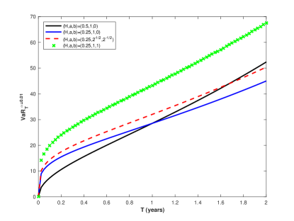
(a) $\alpha=1\%$ and $H=0.25$

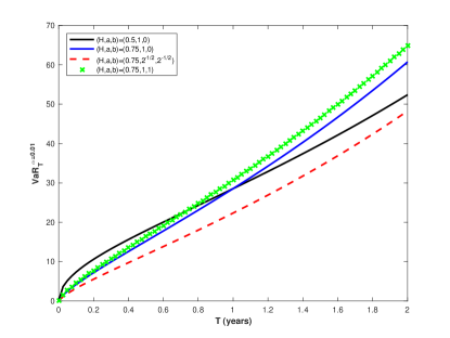
(b) $\alpha=1\%$ and $H=0.75$

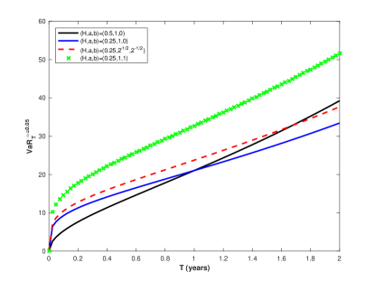
(c) $\alpha=5\%$ and $H=0.25$

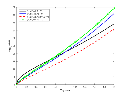
(d) $\alpha=5\%$ and $H=0.75$

Figure 1: Value-at-Risk. $S_{0}=100$, $r=3\%$, and $\sigma=10\%$ were fixed as main parameters.

4.1.2 Expected Shortfall

A weakness of the VaR approach is it only reflects the minimum loss on the portfolio for the quantile $\alpha$. An alternative approach is the Expected Shortfall, a.k.a Conditional VaR [23]. It’s defined as the expected losses for a given VaR level . Mathematically, the Expected Shortfall at level $\alpha$ and time $T$, $\text{ES}_{T}^{\alpha}$ is computed as:

$$\text{ES}_{T}^{\alpha} = S_{0}\text{e}^{rT}-\mathbb{\mathbb{E}}\left(\left.S_{T}\right|S_{T}<VaR_{T}^{\alpha}\right)$$

$$= S_{0}\text{e}^{rT}-\frac{1}{\alpha}\int_{0}^{V}S_{T}P\left(S_{T},T\right)\text{d}S_{T}$$

where $V$ is given by Eq. 16, and:

$$\int_{0}^{V}S_{T}P\left(S_{T},T\right)\text{d}S_{T} = \int_{0}^{V}S_{T}P\left(S_{T},T\right)\text{d}S_{T}$$

$$= \int_{-\infty}^{\ln V-\mu t}\text{e}^{x_{T}+\mu T}P\left(x_{T},T\right)\text{d}x_{T}$$

$$= \frac{{\displaystyle\text{e}^{x_{0}+\mu T}\int_{-\infty}^{\ln V-\mu T}\text{e}^{-\frac{\left(x_{T}-x_{0}-\frac{1}{2}\sigma^{2}\left[\left(a+b\right)^{2}-2^{2H}ab\right]T^{2H}\right)^{2}}{2\sigma^{2}\left[\left(a+b\right)^{2}-2^{2H}ab\right]T^{2H}}}\text{d}x_{T}}}{\sqrt{2\pi\sigma^{2}\left[\left(a+b\right)^{2}-2^{2H}ab\right]T^{2H}}}$$

$$= S_{0}\text{e}^{\mu T}N\left(-\frac{\ln\left(\frac{S_{0}}{V}\right)+\mu T+\frac{1}{2}\sigma^{2}\left[\left(a+b\right)^{2}-2^{2H}ab\right]T^{2H}}{\sigma\sqrt{\left[\left(a+b\right)^{2}-2^{2H}ab\right]T^{2H}}}\right)$$

$$= S_{0}\text{e}^{\mu T}N\left(-d_{1}^{a,b,H,V}\right)$$

with:

$$d_{1}^{a,b,H}=\frac{\ln\left(\frac{S_{0}}{V}\right)+rT+\frac{1}{2}\sigma^{2}\left[\left(a+b\right)^{2}-2^{2H}ab\right]T^{2H}}{\sigma\sqrt{\left[\left(a+b\right)^{2}-2^{2H}ab\right]T^{2H}}}$$

Moreover, since:

$$d_{1}^{a,b,H,V}=d_{2}^{a,b,H,V}+\sigma\sqrt{\left[\left(a+b\right)^{2}-2^{2H}ab\right]T^{2H}}$$

and by virtue of Eq. 15, $-d_{1}^{a,b,H,V}=N^{-1}\left(\alpha\right)$, we arrive at:

$$\text{ES}_{T}^{\alpha}=S_{0}\text{e}^{rT}-S_{0}\frac{\text{e}^{\mu T}}{\alpha}N\left(N^{-1}\left(\alpha\right)-\sigma\sqrt{\left[\left(a+b\right)^{2}-2^{2H}ab\right]T^{2H}}\right)$$

The Fig. 2 reports the Expected Shortfall values related to the VaR evaluates in Fig. 1.

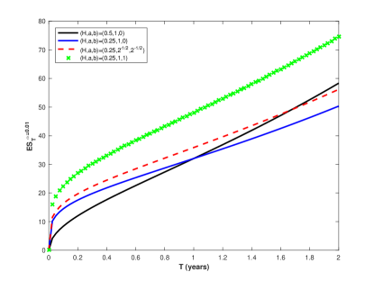
(a) $\alpha=1\%$ and $H=0.25$

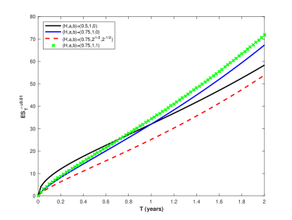
(b) $\alpha=1\%$ and $H=0.75$

(c) $\alpha=5\%$ and $H=0.25$

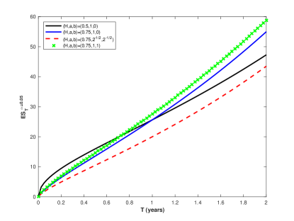
(d) $\alpha=5\%$ and $H=0.75$

Figure 2: Expected Shortfall. $S_{0}=100$, $r=3\%$, and $\sigma=10\%$ were fixed as main parameters.

4.2 European option pricing

As pointed by Zili [18], gfBm is not a semimartingale (unless $H=1/2$). This issue has two-fold: the existence of arbitrage opportunities and the absence of the risk-neutral measure. Nonetheless, we can skip any economical assumptions and obtain the option valuation under the physical measure using the actuarial approach [24], in a similar way how the fair value of an insurance contract is priced. Since $\text{e}^{\mu T}=\frac{\mathbb{E^{P}}\left(S_{T}\right)}{S_{0}}$, the fair premium for a vanilla European Call option with maturity $T$ and exercise price $E$ is given by [24]:

$$\text{CALL}\left(E,T\right)=\mathbb{E^{P}}\left[\left(\text{e}^{-\mu T}S_{T}-\text{e}^{-rT}E\right)^{+}\right]$$

Given that:

$$\text{e}^{-\mu T}S_{T}>\text{e}^{-rT}E \iff \text{e}^{x_{T}}>\text{e}^{-rT}E$$

$$\iff x_{T}>\ln E-rT$$

we have:

$$\text{CALL}\left(E,T\right) = \int_{\ln E-rT}^{\infty}\left(\text{e}^{x_{T}}-\text{e}^{-rT}E\right)P\left(x_{T},T\right)\text{d}x_{T}$$ (17)

$$= \int_{\ln E-rT}^{\infty}\text{e}^{x_{T}}P\left(x_{T},T\right)\text{d}x_{T}-E\text{e}^{-rT}\int_{\ln E-rT}^{\infty}P\left(x_{T},T\right)\text{d}x_{T}$$

Solving each one of the above integrals:

$$\int_{\ln E-rT}^{\infty}\text{e}^{x_{T}}P\left(x_{T},T\right)\text{d}x_{T} = \frac{{\displaystyle\int_{\ln E}^{\infty}\text{e}^{x_{T}}\text{e}^{-\frac{\left(x_{T}-x_{0}+\frac{1}{2}\sigma^{2}\left[\left(a+b\right)^{2}-2^{2H}ab\right]T^{2H}\right)^{2}}{2\sigma^{2}\left[\left(a+b\right)^{2}-2^{2H}ab\right]T^{2H}}}\text{d}x_{T}}}{\sqrt{2\pi\sigma^{2}\left[\left(a+b\right)^{2}-2^{2H}ab\right]T^{2H}}}$$

$$= \frac{{\displaystyle\text{e}^{x_{0}}\int_{\ln E}^{\infty}\text{e}^{-\frac{\left(x_{T}-x_{0}-\frac{1}{2}\sigma^{2}\left[\left(a+b\right)^{2}-2^{2H}ab\right]T^{2H}\right)^{2}}{2\sigma^{2}\left[\left(a+b\right)^{2}-2^{2H}ab\right]T^{2H}}}\text{d}x_{T}}}{\sqrt{2\pi\sigma^{2}\left[\left(a+b\right)^{2}-2^{2H}ab\right]T^{2H}}}$$

$$= S_{0}N\left(\frac{\ln\left(\frac{S_{0}}{E}\right)+rT+\frac{1}{2}\sigma^{2}\left[\left(a+b\right)^{2}-2^{2H}ab\right]T^{2H}}{\sigma\sqrt{\left[\left(a+b\right)^{2}-2^{2H}ab\right]T^{2H}}}\right)$$

$$= S_{0}N\left(d_{1}^{a,b,H,E}\right)$$

$$\int_{\ln E-rT}^{\infty}P\left(x_{T},T\right)\text{d}x_{T} = N\left(\frac{\ln\left(\frac{S_{0}}{E}\right)+rT-\frac{1}{2}\sigma^{2}\left[\left(a+b\right)^{2}-2^{2H}ab\right]T^{2H}}{\sigma\sqrt{\left[\left(a+b\right)^{2}-2^{2H}ab\right]T^{2H}}}\right)$$

$$= N\left(d_{2}^{a,b,H,E}\right)$$

Then,

$$\text{CALL}\left(E,T\right)=S_{0}N\left(d_{1}^{a,b,H,E}\right)-E\text{e}^{-rT}N\left(d_{2}^{a,b,H,E}\right)$$ (18)

It should be noted that the above formula has correspondence with earlier results. If $\left(a,b\right)=\left(1,0\right)$, the pricing yields for the fractional BS formula [3]. While for $a=b=1/\sqrt{2}$ and $c=1$, the valuation formula matches to the sub-fractional BS formula [25]. Moreover, the standard BS formula is recovered using $\left(a,b,H\right)=\left(1,0,1/2\right)$ or $\left(a,b,H\right)=\left(1/\sqrt{2},1/\sqrt{2},1/2\right)$.

Conversely, for European put options, the valuation goes to:

$$\text{PUT}\left(E,T\right) = \mathbb{E^{P}}\left[\left.\left(\text{e}^{-rT}E-\text{e}^{-\mu T}S_{T}\right)^{+}\right|\text{e}^{-\mu T}S_{T}<\text{e}^{-rT}E\right]$$ (19)

$$= \int_{-\infty}^{\ln E-rT}\left(\text{e}^{-rT}E-\text{e}^{x_{T}}\right)P\left(x_{T},T\right)\text{d}x_{T}$$

$$= E\text{e}^{-rT}N\left(-d_{2}^{a,b,H}\right)-S_{0}N\left(-d_{1}^{a,b,H}\right)$$

Fig. 3 shows the European option prices, from formulas 18 and 19, for out-of-the-money Calls and Puts as a function of moneyness ($Ee^{-rT}/S_{0}$); i.e., Put prices for $E<S_{0}e^{rt}$ and Call prices $E<S_{0}e^{rt}$. The plot considers short (6 months in Figs. 3a and 3b) and long maturities (2 years in Figs. 3c and 3d) as well low ( Figs. 3a and 3c) and high (Figs. 3b and 3d) Hurst values. The prices considers the valuation under the proposed model with $a=b=1$ (green cross), but also the reduced cases: the standard Black-Scholes formula (solid black line), the fractional Black-Scholes model (blue dash-dot), and the sub-fractional specification (red dashed line).

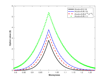
(a) $T=0.5$ and $H=0.25$

(b) $T=0.5$ and $H=0.75$

(c) $T=2$ and $H=0.25$

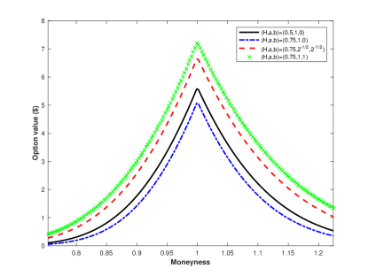
(d) $T=2$ and $H=0.75$

Figure 3: Out-of-the-money European Option prices for the Black-Scholes model driven by gfBm. $S_{0}=100$, $r=3\%$, and $\sigma=10\%$ were fixed as main parameters.

5 A CEV-type extension

Lets consider now a further extension from Eq. (6) where the parameter $\sigma$ is allowed to be level-dependent; i.e., $\sigma=\sigma\left(S_{t}\right)$. In particular, if we assume $\sigma=\sigma_{0}S_{t}^{\frac{\beta}{2}-1}$ with constant $\alpha$, we have a Constant Elasticity of Variance structure, as in the well-known CEV model proposed by Cox [26, 27]. Under generalized fractional CEV model, the price obeys the following SDE:

$$\text{d}S_{t}=\mu S_{t}+\sigma_{0}S_{t}^{\frac{\beta}{2}}\text{d}M_{t}^{H,a,b}$$ (20)

In the limit case, when the elasticity of variance goes to zero ($\beta=2$) , the BS scheme is recovered. Moreover, if we restrict $\beta<2$ the leverage effect arises: inverse relationship between price and volatility commonly observed in equity markets [28]. This direct relation price-volatility is capable to address the smile-skew empirical fact [29]. The rest of the papers considers $\beta<2$.

By the change of variables $y_{t}=S_{t}^{2-\beta}$, the process (20) goes to:

$$y_{t}=\left(2-\beta\right)\sigma\sqrt{y_{t}}\text{d}M_{t}^{H,a,b}+\left(2-\beta\right)\left\{\mu y_{t}+\left(1-\beta\right)\sigma^{2}Ht^{2H-1}\left[\left(a+b\right)^{2}-2^{2H}ab\right]\right\}\mathrm{d}t$$ (21)

According to, the evolution of the transition density function $P=P(y,t)$ obeys the following PDE:

$$\frac{\partial P}{\partial t}=\frac{\partial^{2}}{\partial y^{2}}\left[A(t)yP\right]-\frac{\partial}{\partial y}\left\{\left[By+C(t)\right]P\right\}$$ (22)

with

$$A(t) = \left(2-\beta\right)^{2}\sigma^{2}Ht^{2H-1}\left[\left(a+b\right)^{2}-2^{2H}ab\right]$$

$$B = \left(2-\beta\right)\mu$$

$$C(t) = \frac{\left(1-\beta\right)}{\left(2-\beta\right)}A(t)$$

and initial condition $P(y,0)=\delta\left(y-y_{0}\right)$ and $y_{0}=S_{0}^{2-\beta}$.

For the purpose of solve Eq. (22), and taking advantage of the constant ratio $\theta=\frac{A\left(t\right)}{C\left(t\right)}=\frac{\left(2-\alpha\right)}{\left(1-\alpha\right)}$, we apply the following transformations:

$$\bar{y}=y_{t}\text{e}^{-t\cdot B(t)}$$ (23)

$$\bar{P}=P\text{e}^{-t\cdot B(t)}$$ (24)

$$\bar{t}={\displaystyle\frac{\phi(t)}{2}}$$ (25)

with

$$\phi\left(t\right) = \int_{0}^{t}A\left(\tilde{t}\right)\text{e}^{-B\tilde{t}}\text{d}\tilde{t}$$ (27)

$$\left[\left(a+b\right)^{2}-2^{2H}ab\right]\frac{\sigma^{2}\left(2-\beta\right)^{2}}{2\left(2H+1\right)}\text{e}^{-\left(2-\alpha\right)\beta t}$$

$$\times t^{2H}\left\{2H+1+\text{e}^{\frac{1}{2}\left(2-\beta\right)\mu t}\left[\left(2-\beta\right)\mu t\right]^{-H}M_{H,H+1/2}\left[\left(2-\beta\right)\mu t\right]\right\}$$

and $M_{\kappa,\upsilon}\left(l\right)$ the M-Whittaker function.

Then, after replace in Eq. (22), we obtain the following parabolic equation with constant coefficients:

$$\frac{\partial\bar{P}}{\partial\bar{t}}=-\frac{\partial}{\partial\bar{y}}\left\{2\theta\bar{P}\right\}+\frac{\partial^{2}}{\partial\bar{y}^{2}}\left[2\bar{y}\bar{P}\right]$$ (28)

The above expression matches the Fokker-Planck equation for a time-homogeneous Feller process [30], and in consequence, can be solved analytically. Imposing an absorbing boundary condition at the zero-state (Dirichlet boundary condition at the origin, $P_{x_{t}=0}^{abs}=0$) we arrive at [30, 31]:

$$\bar{P}\left(\left.\bar{y},\bar{t}\right|y_{0},0\right)=\frac{1}{2\bar{t}}\left(\frac{y_{0}}{\bar{y}}\right)^{\frac{1-\vartheta}{2}}\exp\left[-\frac{\left(\bar{y}+y_{0}\right)}{2\bar{t}}\right]I_{1/\left(2-\alpha\right)}\left(\frac{\sqrt{\bar{y}y_{0}}}{\bar{t}}\right)$$ (29)

where $I_{\nu}\left(\bullet\right)$ is the modified Bessel function of the first kind of order $\nu$.

By the reason of Eqs. (23)-(27), the transition density for the process (21) is written as:

$$P\left(\left.S_{t},T\right|S_{0},0\right) =P\left(\left.y_{T},T\right|y_{0},0\right)\frac{\partial y_{T}}{\partial S_{T}}$$

$$=\left(2-\beta\right)k^{\frac{1}{2-\beta}}\left(lm^{1-2\beta}\right)^{\frac{1}{2\left(2-\beta\right)}}\text{e}^{-l-m}I_{1/\left(2-\beta\right)}\left(2\sqrt{lm}\right)$$ (30)

with

$$k = \left[\phi\left(T\right)/2\right]^{-1},$$ (31)

$$l = kS_{0}^{2-\beta}\text{e}^{u\left(2-\beta\right)T}$$ (32)

$$m = kS_{T}^{2-\beta}$$ (33)

Further, with the help of the density (30), and taking conditional expectations for the price process with $\alpha<2$, we can arrive at:

$$\mathbb{E^{P}}\left(S_{T}\right) = \int_{0}^{\infty}S_{T}P\left(S_{T},T\right)\text{d}S_{T}$$

$$= \int_{0}^{\infty}\left(\frac{m}{k}\right)^{\frac{1}{2-\beta}}\left(\frac{l}{m}\right)^{\frac{1}{2\left(2-\beta\right)}}\text{e}^{-l-m}I_{1/\left(2-\beta\right)}\left(2\sqrt{lm}\right)\text{d}m$$

$$= \int_{0}^{\infty}\left(\frac{l}{k}\right)^{\frac{1}{2-\alpha}}\left(\frac{m}{l}\right)^{\frac{1}{2\left(2-\beta\right)}}\text{e}^{-l-m}I_{1/\left(2-\beta\right)}\left(2\sqrt{lm}\right)\text{d}m$$

$$= S_{0}\text{e}^{uT}\int_{0}^{\infty}\underbrace{\left(\frac{2m}{2l}\right)^{\frac{1}{2\left(2-\beta\right)}}\text{e}^{-\frac{2l+2m}{2}}I_{1/\left(2-\beta\right)}\left(\sqrt{\left(2l\right)\left(2m\right)}\right)}_{{\displaystyle f\left(2m;2+\frac{2}{2-\beta},2l\right)}}\text{d}m$$

$$= S_{0}\text{e}^{uT}$$

The last step is achieved taking in account that $f\left(u;\nu,\lambda\right)=\left(u/\lambda\right)^{\frac{\nu-2}{4}}\text{e}^{-\left(x+\lambda\right)/2}I_{\nu}\left(\sqrt{x\lambda}\right)$ matches to the density function for the non-central chi-square distribution with non-centrality parameter $\lambda$ and $\nu$degree of freedoms, $u\sim\chi_{\nu}^{2}\left(\lambda\right)$, and its complementary function defined as:

$$\int_{a}^{\infty}f\left(u;\nu,\lambda\right)\text{d}u=Q\left(a;\nu,\lambda\right)$$

where $Q\left(0;\nu,\lambda\right)=1$.

Applying the arguments discussed in section 3, for $\alpha<2$, and since $S_{T}\text{e}^{-\mu T}>E\text{e}^{-rT}\iff S_{T}>E\text{e}^{\left(\mu-r\right)t}$, the pricing for an European Call option is computed as:

$$\text{CALL}\left(E,T\right) = \mathbb{E^{P}}\left[\left(\text{e}^{-\mu T}S_{T}-\text{e}^{-rT}E\right)^{+}\right]$$ (34)

$$= \int_{E\text{e}^{\mu T-rT}}^{\infty}\left(\text{e}^{-\mu T}S_{T}-\text{e}^{-rT}E\right)P\left(S_{T},T\right)\text{d}S_{T}$$

where,

$$\int_{E\text{e}^{\mu T-rT}}^{\infty}\text{e}^{-\mu T}S_{T}P\left(S_{T},T\right)\text{d}S_{T} = \text{e}^{-\mu T}\int_{kE^{2-\beta}\text{e}^{\left(2-\beta\right)\left(u-r\right)T}}^{\infty}\left(\frac{m}{k}\right)^{\frac{1}{2-\beta}}\left(\frac{l}{m}\right)^{\frac{1}{2\left(2-\beta\right)}}$$

$$\times\text{e}^{-l-m}I_{1/\left(2-\beta\right)}\left(2\sqrt{lm}\right)\text{d}m$$

$$= S_{0}\int_{kE^{2-\beta}\text{e}^{\left(2-\beta\right)\left(u-r\right)T}}^{\infty}\left(\frac{2m}{2l}\right)^{\frac{1}{2\left(2-\beta\right)}}\text{e}^{-\frac{2l+2m}{2}}$$

$$\times I_{1/\left(2-\beta\right)}\left(\sqrt{\left(2l\right)\left(2m\right)}\right)\text{d}m$$

$$= S_{0}\int_{F}^{\infty}{\displaystyle f\left(2m;2+\frac{2}{2-\beta},2l\right)}\text{d}m$$

$$= S_{0}Q\left(2F;2+\frac{2}{2-\beta},2l\right)$$

being $F=kE^{2-\beta}\text{e}^{\left(2-\beta\right)\left(u-r\right)T}$. Moreover,

$$\int_{E\text{e}^{\mu T-rT}}^{\infty}E\text{e}^{-rT}P\left(S_{T},T\right)\text{d}S_{T} = E\text{e}^{-rT}\int_{F}^{\infty}{\displaystyle f\left(2l;2+\frac{2}{2-\beta},2m\right)}\text{d}m$$

Making use of the property [32]:

$$\int_{a}^{\infty}{\displaystyle f\left(2u;2v,2\lambda\right)\text{d}\lambda}=1-Q\left(2u;2v-2,2a\right)$$

we get:

$$\int_{F}^{\infty}{\displaystyle f\left(2l;2+\frac{2}{2-\beta},2m\right)}\text{d}m=1-Q\left(2l;\frac{2}{2-\beta},2F\right)$$

Then, after replace on Eq. 34 the Call valuation goes to:

$$\text{CALL}\left(E,T\right)=S_{0}Q\left(2F;2+\frac{2}{2-\beta},2l\right)-E\text{e}^{-rT}\left[1-Q\left(2l;\frac{2}{2-\beta},2F\right)\right]$$ (35)

Analogously, for an European put, we arrive at:

$$\text{PUT}\left(E,T\right)=E\text{e}^{-rT}Q\left(2l;\frac{2}{2-\alpha},2F\right)-S_{0}\left[1-Q\left(2F;2+\frac{2}{2-\alpha},2l\right)\right]$$

6 Summary

In this paper we have used the gfBm as the driven process in the price fluctuations modeling. By means of the related both Ito calculus and effective Fokker-Planck equation, we have obtained the analytical valuation for risk measures as Value-at-Risk and Expected Shortfall, as well the close-form European Call pricing formulas for the generalized fractional BS model. In addition, the CEV extension is discussed derived its transition density and option pricing. Since that gmfBm is a generalization for both Bm, fBm, and sfBm; we can recovery the the classical results for the BS model, but also their fractional and sub-fractional extensions. The study of exotic options as well the inclusion of stochastic volatility models is pending to address in the future.

References

• [1] F. Black and M. Scholes, “The pricing of options and corporate liabilities”, J. Polit. Econ. 81 (1973) 637–654.
• [2] B. B. Mandelbrot and J. W. Van Ness, “Fractional Brownian motions, fractional noises and applications”, SIAM Rev. 10 (1968) 422–437.
• [3] C. Necula, “Option pricing in a fractional Brownian motion environment”, Working paper, Bucharest, 2002.
• [4] Y. Hu and B. Øksendal, “Fractional white noise calculus and applications to finance”, Infin. Dimens. Anal. Quantum Probab. Relat. Top. 6 (2003) 1–32.
• [5] D. Ahmadian and L. V. Ballestra, “Pricing geometric Asian rainbow options under the mixed fractional Brownian motion”, Physica A 555 (2020) 124458.
• [6] A. A. Araneda, “The fractional and mixed-fractional CEV model”, J. Comput. Appl. Math. 363 (2020) 106–123.
• [7] A. A. Araneda, “Credit default swaps and the mixed-fractional CEV model”, arXiv:2211.07564 .
• [8] P. Cheng, Z. Xu and Z. Dai, “Valuation of vulnerable options with stochastic corporate liabilities in a mixed fractional Brownian motion environment”, Mathematics and Financial Economics 17 (2023) 429–455.
• [9] W.-G. Zhang, Z. Li, Y.-J. Liu and Y. Zhang, “Pricing European option under fuzzy mixed fractional Brownian motion model with jumps”, Computational Economics 58 (2021) 483–515.
• [10] T. Bojdecki, L. G. Gorostiza and A. Talarczyk, “Sub-fractional Brownian motion and its relation to occupation times”, Stat. Prob. Lett. 69 (2004) 405–419.
• [11] C. Tudor, “Some properties of the sub-fractional Brownian motion”, Stochastics 79 (2007) 431–448.
• [12] F. Xu and S. Zhou, “Pricing of perpetual American put option with sub-mixed fractional Brownian motion”, Fract. Calc. Appl. Anal. 22 (2019) 1145–1154.
• [13] W. Wang, G. Cai and X. Tao, “Pricing geometric Asian power options in the sub-fractional brownian motion environment”, Chaos Solit. Fractals 145 (2021) 110754.
• [14] B. Ji, X. Tao and Y. Ji, “Barrier option pricing in the sub-mixed fractional brownian motion with jump environment”, Fractal and Fractional 6 (2022) 244.
• [15] X. Wang, Z. Yang, P. Cao and S. Wang, “The closed-form option pricing formulas under the sub-fractional Poisson volatility models”, Chaos Solit. Fractals 148 (2021) 111012.
• [16] L. Tao, Y. Lai, Y. Ji and X. Tao, “Asian option pricing under sub-fractional Vasicek model”, Quant. Financ. Econ. 7 (2023) 403–419.
• [17] A. A. Araneda and N. Bertschinger, “The sub-fractional CEV model”, Physica A 573 (2021) 125974.
• [18] M. Zili, “Generalized fractional Brownian motion”, Mod. Stoch.: Theory Appl. 4 (2017) 15–24.
• [19] M. Zili, “On the generalized fractional Brownian motion”, Math. Models Comput. Simul. 10 (2018) 759–769.
• [20] D. Nualart and M. S. Taqqu, “Wick–Itô formula for regular processes and applications to the Black and Scholes formula”, Stochastics 80 (2008) 477–487.
• [21] L. Yan, G. Shen and K. He, “Itô’s formula for a sub-fractional Brownian motion”, Commun. Stoch. Anal. 5 (2011) 9.
• [22] C. Bender, “An Itô formula for generalized functionals of a fractional Brownian motion with arbitrary Hurst parameter”, Stoch. Process. Their. Appl. 104 (2003) 81–106.
• [23] P. Artzner, F. Delbaen, J.-M. Eber and D. Heath, “Coherent measures of risk”, Mathematical finance 9 (1999) 203–228.
• [24] M. Bladt and T. H. Rydberg, “An actuarial approach to option pricing under the physical measure and without market assumptions”, Insur Math Econ 22 (1998) 65–73.
• [25] C. Tudor, “Sub-fractional Brownian motion as a model in finance”, Working paper, University of Bucharest, 2008.
• [26] J. C. Cox, “Notes on option pricing I: Constant elasticity of variance diffusions”, 1975., working paper, Stanford University.
• [27] J. C. Cox, “The constant elasticity of variance option pricing model”, J. Portf. Manag. 23 (1996) 15–17.
• [28] L. V. Ballestra and L. Cecere, “A numerical method to estimate the parameters of the CEV model implied by American option prices: Evidence from NYSE”, Chaos, Solitons & Fractals 88 (2016) 100–106.
• [29] V. Linetsky and R. Mendoza, “Constant elasticity of variance (CEV) diffusion model”, in Encyclopedia of Quantitative Finance, ed. R. Cont (John Wiley & Sons, Ltd, 2010).
• [30] W. Feller, “Two singular diffusion problems”, Ann. Math. (1951) 173–182.
• [31] A. E. Lindsay and D. R. Brecher, “Simulation of the CEV process and the local martingale property”, Math. Comput. Simulat. 82 (2012) 868–878.
• [32] M. Schroder, “Computing the constant elasticity of variance option pricing formula”, J. Finance 44 (1989) 211–219.