A functional skeleton transfer

Abstract.

The animation community has spent significant effort trying to ease rigging procedures. This is necessitated because the increasing availability of 3$D$ data makes manual rigging infeasible. However, object animations involve understanding elaborate geometry and dynamics, and such knowledge is hard to infuse even with modern data-driven techniques. Automatic rigging methods do not provide adequate control and cannot generalize in the presence of unseen artifacts. As an alternative, one can design a system for one shape and then transfer it to other objects. In previous work, this has been implemented by solving the dense point-to-point correspondence problem. Such an approach requires a significant amount of supervision, often placing hundreds of landmarks by hand. This paper proposes a functional approach for skeleton transfer that uses limited information and does not require a complete match between the geometries. To do so, we suggest a novel representation for the skeleton properties, namely the functional regressor, which is compact and invariant to different discretizations and poses. We consider our functional regressor a new operator to adopt in intrinsic geometry pipelines for encoding the pose information, paving the way for several new applications. We numerically stress our method on a large set of different shapes and object classes, providing qualitative and numerical evaluations of precision and computational efficiency. Finally, we show a preliminar transfer of the complete rigging scheme, introducing a promising direction for future explorations.

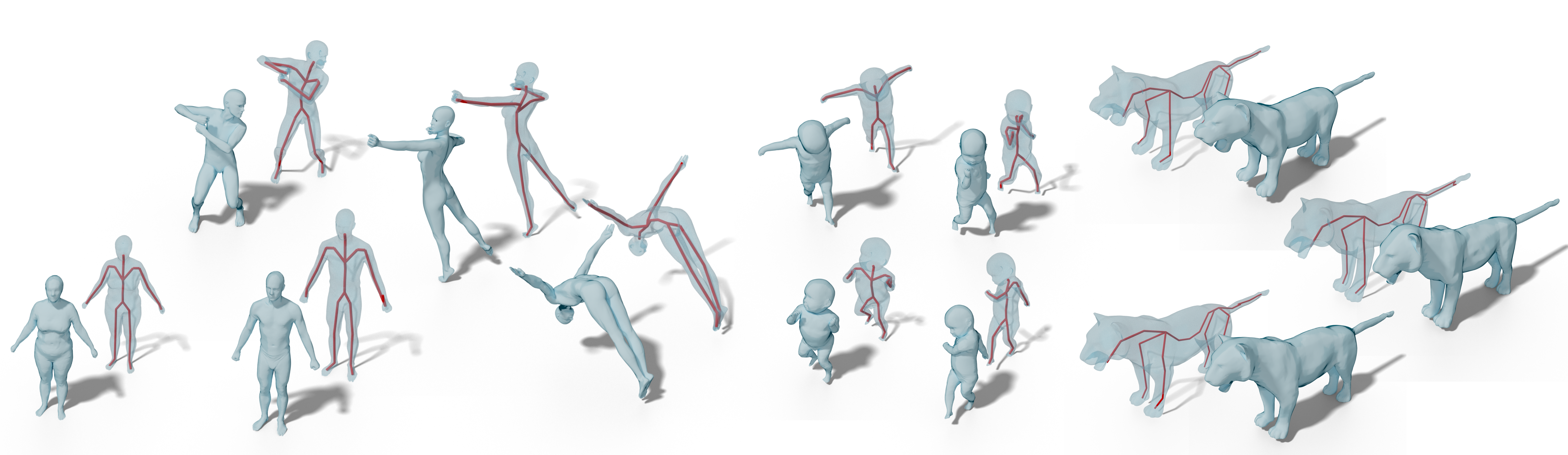
Figure 1. Some results of our method. On the left, five adult humans that inherited the SMPL (Loper et al., 2015) skeleton; these surfaces come from different datasets and have different discretizations. In the middle, four children shapes on which we transfer the skeleton from SMIL (Hesse et al., 2018). On the right, three lions that received the skeleton from SMAL (Zuffi et al., 2017).

1. Introduction

Animating a 3D object is a time-consuming and challenging problem; it requires matching the expectations suggested by our experience and balancing the trade-off between usability and expressiveness. Also, a coherent rigging system across similar objects is desirable to allow reuse of animations with little effort.

Several methods have been proposed to solve the automatic rigging of meshes. They rely on algorithms that process the geometric structure (Jacobson et al., 2012) or, more recently, by learning using data-driven approaches (Rajendran and Lee, 2020). However, they hardly produce coherent results among arbitrary objects and do not provide the user with additional information about the semantics and the structural role of each component of the shape. To keep a degree of control, another approach is defining a rigging system and transferring it to other models, but this is commonly achieved by establishing a dense point-to-point correspondence, which requires user annotations. Also, determing point-to-point correspondence is one of the fundamental open problems of geometry processing, particularly when facing non-isometric objects.

In this work, we claim that the skeleton can be accurately transferred by a functional approach without relying on a dense point-to-point correspondence. Our pipeline asks the user to define a rigged system for one shape. Then, we optimize for a regressor that is parsed to a functional representation, and finally, it is transferred to other shapes. This representation offers a new perspective in skeleton encoding; it is compact and entirely intrinsic (i.e., it does not change with varying poses of the subject). Given a new shape to animate, we ask for a few landmarks on the target object (seven on humans and which, in practice, can be detected almost automatically) and we rely on the Functional Maps framework (Nogneng and Ovsjanikov, 2017) to transfer our rigging. This framework is state-of-the-art for the functional transferring task, both in terms of performance and efficiency. Our approach produces results coherent across different objects of the same class, as shown in Figure 1. Finally, we cannot find implementations for previous methods; we consider this one of the main reasons for proposing novel approaches. The code and data used in this paper will be made entirely available for research purposes.

To summarize, our contribution is threefold:

1. We propose the first functional pipeline for skeleton transfer. It produces accurate results efficiently and with limited user input. It is general across different settings and object classes.

2. We introduce a new spectral representation for the shape skeleton information; that is compact, entirely intrinsic, and invariant to different discretizations and poses of the subject. This representation provides a new perspective to analyze object mechanics.

3. We will release all the code and data used in our experiments.

2. State of the art

2.1. Classical methods

Several researchers have tried to define the skeleton for a given shape by using automatic systems. One of the fundamental works in this field is Pinocchio (Baran and Popović, 2007) by Baran and Popovic; the proposed pipeline produces an animation-ready character starting from a generic object. This process is divided into two steps: skeleton embedding and skin attachment.

Some works (Gleicher, 1998), (Lee and Shin, 1999), (Choi and Ko, 2000) solve kinematic constraints on joint positions using displacement maps. In (Allen et al., 2003), the authors provide joint retargeting through the use of three markers. The distance between the joints and the markers should be fixed. However, this method works only on near-similar morphological bodies. Methods like (Capell et al., 2005) and (Orvalho et al., 2008) introduced the transferring of the rig. The first is not compatible with common skinning methods, and the second can only be applied to a limited set of characters. In (Seo et al., 2010), the authors provide a method based on data mapping applicable to surfaces and volumes, but a careful manual selection of points is necessary to initialize the correspondence.

2.2. Automatic Rigging and rigging transfer

The main disadvantage of automatic rigging methods is that the animation sequence should be designed on a specific skeleton. Instead, the rigging transfer methods tackled this problem by transferring a native skeleton with an attached animation, combining it to the new shape. Several works focus on the transfer of the medial-axis (Yang et al., 2018) (Seylan and Sahillioğlu, 2019), which is the set of points having more than one closest point to the boundary of a shape. The medial axis of a 3D object can be expressed both as a curve and as a 2D surface. However, medial axis methods are not compatible with standard render engines, and they are computationally inefficient.

Another approach explored in (Le and Deng, 2012) and (Le and Deng, 2014) employs example-based methods to automatically generate linear blend skinning models. The method takes as input a sequence of poses of a model and it outputs the skeleton, the skinning weights and the bone transformations. The output is compatible with common game engines and 3D modelling software, however, such a sequence of shapes is not always easy to have since requires data acquisition from a real-world scenario and the method largely depends on the quality of input example meshes.

2.3. Motion transfer

Other approaches (Liu et al., 2018), (Basset et al., 2019) propose to transfer each pose of a 3D shape to another using a non-rigid registration. In these methods, a further adjustment is required to have a smooth animation from the sequence of poses obtained. A more promising procedure involves deforming a shape to adapt to a rigged one, applying the given skeleton to the deformed shape. In (Marin et al., 2020), (Melzi et al., 2020) and (Ni et al., 2020), the authors made a non-rigid registration from a source shape to a target one, and then transfer the skinning information. A similar work (Jin et al., 2018) introduces the idea of aura mesh, a volume that surrounds the character and permits avoidance of self-collisions. The rigless methods (Basset et al., 2019) do not need the post-processing angle correction, but they require additional steps to obtain an animation-ready shape as output. In (Avril et al., 2016) the authors compute a pointwise matching between the two shapes to transfer all the properties of an animation setup. This method requires the manual input of more than 300 key points to initialize the dense correspondence. Then, a regression matrix is estimated to compute the joint positions of the new shape. In addition to the high amount of user input, the method requests the two shapes to be in the same pose. A joint-regressor was also introduced for the SMPL morphable model (Loper et al., 2015), but it requires learning from a large dataset of 3D shapes. Furthermore, the joint-regressor of SMPL is defined pointwise, hence its transfer would require a dense point-to-point correspondence.

3. Background

3.1. LBO basis on shape

\begin{overpic}[trim=0.0pt 0.0pt 0.0pt 0.0pt,clip,width=429.28616pt]{figures/function.png} \put(5.0,-2.0){\scriptsize$\mathcal{M}$} \put(25.0,-2.0){\scriptsize$f$} \put(38.0,-2.0){\scriptsize$\Phi_{0}$} \put(52.0,-2.0){\scriptsize$\Phi_{1}$} \put(65.0,-2.0){\scriptsize$\Phi_{2}$} \put(78.0,-2.0){\scriptsize$\Phi_{3}$} \put(90.0,-2.0){\scriptsize$\Phi_{4}$} \par\put(31.0,8.0){\scriptsize=} \put(43.5,8.0){\scriptsize$\alpha_{1}+$} \put(56.5,8.0){\scriptsize$\alpha_{2}+$} \put(69.5,8.0){\scriptsize$\alpha_{3}+$} \put(82.5,8.0){\scriptsize$\alpha_{4}+$} \par\put(97.0,8.0){\scriptsize\ldots} \put(16.5,12.8){\tiny 0} \put(15.7,11.5){\tiny-0.2} \put(16.0,10.2){\tiny 1.2} \put(16.3,7.0){\tiny\ldots} \put(15.7,0.5){\tiny-1.4} \par\put(27.8,5.0){\tiny max} \put(27.8,1.0){\tiny min} \end{overpic}

Figure 2. Here we visualize some of the functional quantities we referred into the text. Given a geometry $\mathcal{M}$, a function $f$ is a vector that associates a scalar value to each point of the surface. Such function can be decomposed for some basis $\mathbf{\Phi}$ (e.g. the LBO eigenfunctions) recovering a list of coefficients $\alpha$.

We describe $2$-dimensional surfaces embedded in $\mathbb{R}^{3}$ as compact and connected 2-dimensional Riemannian manifolds. Given a surface $\mathcal{M}$, we consider $\mathcal{F}(\mathcal{M}):=\{f:\mathcal{M}\rightarrow\mathbb{R}\}$ as the space of real-valued functions defined over it. In other words, a function $f\in\mathcal{F}(\mathcal{M})$ associates at every point $x\in\mathcal{M}$ a real value $f(x)\in\mathbb{R}$. In the discrete setting, we encode the shape $\mathcal{M}$ in a triangular mesh, defined by the 3D coordinates of its $n_{\mathcal{M}}$ vertices $X_{\mathcal{M}}\in\mathbb{R}^{n_{M}\times 3}$ and the list of the edges $E_{\mathcal{M}}$ that connect these vertices generating triangular faces. We associate to each mesh the cotangent Laplace-Beltrami operator (LBO), that is discretized by a $n_{\mathcal{M}}\times n_{\mathcal{M}}$ matrix (Meyer et al., 2003). We collect the first $k$ eigenfunctions of the LBO of $\mathcal{M}$ (the ones associated to the $k$ smallest eigenvalues) as columns in a matrix $\bm{\Phi}_{k_{\mathcal{M}}}=\big{[}\phi_{1},\phi_{2},\cdots,\phi_{k_{\mathcal{M}}}\big{]}$. In geometry processing, these eigenfunctions are widely used to approximate functions or signals defined on 3D shapes extending Fourier analysis on non-Euclidean domains (Taubin, 1995; Lévy, 2006; Vallet and Lévy, 2008). In particular, functions can be represented by a linear combination of the basis $\bm{\Phi}_{k_{\mathcal{M}}}$ as $\tilde{f}=\bm{\Phi}_{k_{\mathcal{M}}}\bm{\widehat{f}}$, where $\bm{\widehat{f}}$ are the basis coefficients. Since just a subset of the eigenfunctions is used, this is just an approximation of $f$. The coefficients $\bm{\widehat{f}}$ can be obtained by the projection $\bm{\widehat{f}}=\bm{\Phi}_{k_{\mathcal{M}}}^{\dagger}f$, where $\bm{\Phi}_{k_{\mathcal{M}}}^{\dagger}$ is the Moore–Penrose pseudo-inverse (i.e. $\bm{\Phi}_{k_{\mathcal{M}}}^{\dagger}\bm{\Phi}_{k_{\mathcal{M}}}=Id_{k_{\mathcal{M}}\times k_{\mathcal{M}}}$). The matrix $\bm{\Phi}_{k_{\mathcal{M}}}^{\dagger}$ could be seen as the operator that projects the pointwise values of the function into its Fourier representation. We will exploit this projection through the paper, and we refer to this space of the Fourier coefficients as the functional representation of quantities defined pointwise on the mesh. A visualization of these quantities is shown in Figure 2.

3.2. Functional Maps

A correspondence $T$ between two surfaces $\mathcal{N}$ and $\mathcal{M}$ is a mapping that associates to each point $p\in\mathcal{N}$ the corresponding point $T(p)\in\mathcal{M}$. In the discrete case, we can encode this mapping in a matrix $\Pi_{\mathcal{N}\mathcal{M}}\in\mathbb{R}^{n_{\mathcal{M}}\times n_{\mathcal{N}}}$ such that $\Pi(i,j)=1$ if the $j$-th vertex of the shape $\mathcal{N}$ corresponds to the $i$-th vertex of the shape $\mathcal{M}$ and $\Pi(i,j)=0$ otherwise. From a functional perspective, any function $f\in\mathcal{F}(\mathcal{M})$ could be transferred to a function $g=f\circ T\in\mathcal{F}(\mathcal{N})$. Hence, given the truncated bases $\bm{\Phi}_{k_{\mathcal{M}}}$ and $\bm{\Psi}_{k_{\mathcal{N}}}$ obtained from the eigendecomposition of the LBO respectively of $\mathcal{M}$ and $\mathcal{N}$, the Functional Maps framework (Ovsjanikov et al., 2012) exploits these truncated bases to encode this mapping in a compact matrix $\bm{C}\in\mathbb{R}^{k_{\mathcal{N}}\times k_{\mathcal{M}}}$ referred as a functional map. The matrix $\bm{C}$ can be directly derived from $\Pi$ with the following equation $\bm{C}=\bm{\Psi}_{k_{\mathcal{N}}}^{\dagger}\Pi_{\mathcal{N}\mathcal{M}}\bm{\Phi}_{k_{\mathcal{M}}}$. Once we have a functional map $\bm{C}$, we can recover the correspondence $T$ by transfering an indicator function for each vertex, but (Ovsjanikov et al., 2012) show that this is equivalent to the nearest-neighbour assignment problem between $\bm{\Phi}_{k_{\mathcal{M}}}\bm{C}^{\top}$ and $\bm{\Psi}_{k_{\mathcal{N}}}$. Different strategies and constraints have been proposed to solve for the matrix $\bm{C}$ (Ovsjanikov et al., 2012; Nogneng and Ovsjanikov, 2017; Nogneng et al., 2018; Ren et al., 2019, 2018). Several attempts have also been implemented to extract and refine the pointwise correspondence from the functional representation (Rodolà et al., 2015; Ezuz and Ben-Chen, 2017; Melzi et al., 2019b; Ren et al., 2020; Pai et al., 2021). They produce meaningful results, but the conversion to pointwise maps induces distortions even for accurate functional maps. Here, we adopt the method proposed in (Nogneng and Ovsjanikov, 2017) following the procedure described in (Melzi et al., 2019b).

4. Method

\begin{overpic}[trim=0.0pt 0.0pt 0.0pt 0.0pt,clip,width=429.28616pt]{figures/pipeline2.png} \put(8.0,15.0){Input} \put(26.0,15.0){Target} \put(41.0,18.0){Functional} \put(41.0,15.0){Optimization} \put(64.0,18.0){Functional} \put(66.0,15.0){Map} \put(78.0,18.0){Skeleton Transfer} \end{overpic}

Figure 3. This figure depicts our pipeline overview. Our method inputs are an initial rigged model and a target mesh. Then, we perform optimization to obtain the functional representation of the mesh skinning, and by computing a functional map between the two, we can transfer the skeleton to the target. The transfer lets us move the target following the semantic of the source.

Here we describe our functional-based representation and its relation to the spatial one. Then, we present our algorithm for skeleton transfer, summarized by Figure 3.

4.1. Functional Regressor

A common choice is defining the skeleton $\bm{J}_{\mathcal{M}}\in\mathbb{R}^{Q\times 3}$ as a function of the given surface $\mathcal{M}$, namely the joint regressor. Following (Loper et al., 2015) it can be expressed as a linear operator $\bm{R}\in\mathbb{R}^{Q\times n_{\mathcal{M}}}$, that acts on the coordinates of the vertices $X_{\mathcal{M}}$ in the discrete setting; hence:

(1) $$\bm{J}_{\mathcal{M}}=\bm{R}X_{\mathcal{M}}.$$

We refer to $\bm{R}$ as the standard or spatial regressor.

Starting from this, we propose a novel functional formulation. We can consider the coordinates of the vertices of the meshes $X_{\mathcal{M}}$ as a set of three functions (one for each column) and project them in the space of the Fourier coefficients:

(2) $$\widehat{X}_{\mathcal{M}} =\bm{\Phi}_{k_{\mathcal{M}}}^{\dagger}X_{\mathcal{M}}$$

where the coefficients $\widehat{X}_{\mathcal{M}}\in\mathbb{R}^{k_{\mathcal{M}}\times 3}$.

\begin{overpic}[trim=0.0pt 0.0pt 0.0pt 0.0pt,clip,width=429.28616pt]{figures/regressor.png} \put(101.0,0.0){0} \put(101.0,12.0){6} \par\put(20.0,35.0){$\mathbf{J_{\mathcal{M}}}$} \put(75.0,35.0){$\widehat{\bm{R}}^{2}$} \end{overpic}

Figure 4. On the left, the defined skeleton. On the right, the functional regressor.

Motivation. Since our functional representation is defined on the low-pass filtering of the 3D coordinates, it captures the global structure of the shape, with resilience to high-frequency details. Also, it is intrinsic; it is agnostic to the subject pose and placement in the 3D space. Moreover, it is compact: a spatial joint regressor is encoded by a matrix $n_{\mathcal{M}}\times Q$; our functional regressor has dimension $k_{\mathcal{M}}\times Q$. We generally select $k_{\mathcal{M}}\in[30,200]$; smaller than $n_{\mathcal{M}}$ by at least two orders of magnitude.

In this functional representation, we want to find a linear operator $\widehat{\bm{R}}$ such that:

(3) $$\bm{J}_{\mathcal{M}} =\widehat{\bm{R}}\widehat{X}_{\mathcal{M}}$$

where we refer to $\widehat{\bm{R}}\in\mathbb{R}^{Q\times k_{\mathcal{M}}}$, as the functional or spectral regressor. A visualization of the functional regressor is reported in Figure 4; each column represents a dimension of the LBO basis (one of the eigenfunctions), and each row a different joint. Further comments and analysis are shown in Section 6.

Relation between spectral and standard regressor. Let us consider a single shape $\mathcal{M}$ with its 3D coordinates $X_{\mathcal{M}}$, its LBO eigenfunctions $\bm{\Phi}_{k_{\mathcal{M}}}$, and the Fourier coefficients of its coordinates $\widehat{X}_{\mathcal{M}}$. From Equation 3 and from $\bm{J}_{\mathcal{M}}=\bm{R}X_{\mathcal{M}}$, we can write:

(4) $$\bm{J}_{\mathcal{M}}=\bm{R}X_{\mathcal{M}}\approx\widehat{\bm{R}}\widehat{X}_{\mathcal{M}}=\widehat{\bm{R}}\bm{\Phi}^{\dagger}_{k_{\mathcal{M}}}X_{\mathcal{M}},$$

from which we obtain:

(5) $$\bm{R}\approx\widehat{\mathbf{R}}\bm{\Phi}^{\dagger}_{k_{\mathcal{M}}}.$$

From the definition of the Moore–Penrose pseudo-inverse we have:

(6) $$\bm{R}\bm{\Phi}_{k_{\mathcal{M}}}\approx\widehat{\bm{R}}\underbrace{\bm{\Phi}_{k_{\mathcal{M}}}^{\dagger}\bm{\Phi}_{k_{\mathcal{M}}}}_{Id_{k_{\mathcal{M}}\times k_{\mathcal{M}}}}=\widehat{\bm{R}},$$

and finally we can derive these two relations:

(7) $$\bm{R} \approx\widehat{\bm{R}}\bm{\Phi}^{\dagger}_{k_{\mathcal{M}}}$$

(8) $$\widehat{\bm{R}} \approx\bm{R}\bm{\Phi}_{k_{\mathcal{M}}}.$$

4.2. Skeleton transfer algorithm

ALGORITHM 1 Skeleton Transfer

1:Input: A rigged shape $\mathcal{M}$, a target shape $\mathcal{N}$, and a set of seven landmarks

2:Step 1: Estimate the spatial regressor $\bm{R}$ by optimizing the energy $E$

3:Step 2: Compute the FMAP $\bm{C}$ using the given landmarks

4:Step 3: Convert the spatial regressor $\bm{R}$ in the functional representation $\widehat{\bm{R}}$

5:Step 4: Compute $\bm{J}_{\mathcal{N}}$ using the transferred spectral regressor

6:Output: A skeleton $\bm{J}_{\mathcal{N}}$ for the target shape $\mathcal{N}$

We consider a model $\mathcal{M}$ that is animation-ready, composed by a triangular mesh represented by $n_{\mathcal{M}}$ vertices $X_{\mathcal{M}}\in\mathbb{R}^{n_{\mathcal{M}}\times 3}$ and equipped with a skeleton $\bm{J}_{\mathcal{M}}\in\mathbb{R}^{Q\times 3}$ composed by $Q$ joints. The SMPL model proposed in (Loper et al., 2015) is one possible model that we consider in our experiments. Our objective is to transfer the rigging of $\mathcal{M}$ to a new shape $\mathcal{N}$ represented by a triangular mesh with $n_{\mathcal{N}}$ vertices $X_{\mathcal{N}}\in\mathbb{R}^{n_{\mathcal{N}}\times 3}$. As additional information, we require some landmarks that for the human case are seven. Five of them are located on protrusions and can be automatically computed exploiting the method proposed in (Marin et al., 2020). The remaining two are on the front and the back of the torso. In our experiments, we select them manually since this requires just a few seconds.

Step 1: Spatial Regressor Optimization We want to compute the mesh skeleton through a linear operator $\widehat{\bm{R}}$ defined over the Fourier coefficients of the 3D coordinates of the vertices of the input mesh. To do so, we first obtain a standard regressor $\bm{R}$ as the solution of an optimization defined as the linear combination of 4 energies.

Reconstruction Term.

The first energy asks that the regressor $\bm{R}$ returns the correct position of the joints:

(9) $$E_{rec}=\left\|\bm{R}X_{\mathcal{M}}-\bm{J}_{\mathcal{M}}\right\|^{2}.$$

Locality Term.

To have a regressor invariant to pose, each joint should depend only on the vertices linked by a rigid relation to it, i.e. by a near set of them. To do so, we define a mask matrix $F\in\mathbb{R}^{Q\times n_{\mathcal{M}}}$, that has $F(q,i)=1$ if the position of the vertex $v_{i}$ influences the position of the joint $J_{q}$ and $0$ otherwise. To select which vertices should affect the joint position, we took the ones in the intersection between the non-zero skinning weights belonging to each joint and its hierarchical parent. The resulting set is near to the joint, and so we selected them to populate $F$. We decided to choose the vertices between the joint and its parent since they are near the joint and they have low weights so the deformation of these vertices is low changing between a pose and another. Then, the energy is:

(10) $$E_{loc}=\left\|\bm{R}\odot F-\bm{R}\right\|^{2}$$

where $\odot$ is the element-wise product.

Sparsity Term.

While $E_{loc}$ guarantees that joints are affected by a limited set of vertices, nothing has been imposed on the entries of $R$ that correspond to zero values in the mask $F$. For this reason, we promote zero-values in all these entries that should not contribute to the computation of $\bm{J}_{\mathcal{M}}$:

(11) $$E_{spa}=\||F-\mathbf{1}|\odot\bm{R}\|^{2},$$

where $\mathbf{1}$ is a matrix with the same size of $F$, the entries of which are all equal to $\mathbf{1}$.

Convexity Term.

We observed in our experiment that requiring the weights of each joint to sum to 1 helps to obtain joints inside the mesh boundaries, even if we do not explicitly require that all the weights are non negative. We implement this through the following energy:

(12) $$E_{con}=\left\|\bm{R}e_{n_{\mathcal{M}}}-e_{Q}\right\|^{2}$$

where $e_{n_{\mathcal{M}}}$ and ${e_{Q}}$ are vectors of ones with length $n_{\mathcal{M}}$ and the number of joints respectively.

Optimization formulation.

The optimization to recover the desired regressor is obtained by a linear combination of these four energies:

(13) $$E=\omega_{rec}*E_{rec}+\omega_{loc}*E_{loc}+\omega_{spa}*E_{spa}+\omega_{con}*E_{con}$$

where $\omega_{rec}$, $\omega_{loc}$, $\omega_{spa}$, $\omega_{con}$ are positive real numbers that act as weights. We empirically set them to $\omega_{rec}=1$, $\omega_{loc}=10e3$, $\omega_{con}=1$ and $\omega_{spa}=100$. Putting high weights on $E_{loc}$ and $E_{spa}$ forces the regressor to better compute the joints location as a function of the vertices selected by $F$. These dependencies between each joint and the vertices are independent across the different joints. Apart from setting a rough balance between energies, no exhaustive research has been done.

Implementation.

We use the Tensorflow auto-differentiation library to solve this problem, relying on the Adam optimizer with a learning rate of $0.1$ and using 1000 iterations.

Step 2: Functional Maps computation Given a new shape $\mathcal{N}$ for which the rigging is not available, our goal is to transfer the regressor from $\mathcal{M}$ to $\mathcal{N}$. Hence, we estimate a functional map $\bm{C}$ between $\mathcal{F}(\mathcal{M})$ and $\mathcal{F}(\mathcal{N})$ following the procedure proposed in (Nogneng and Ovsjanikov, 2017). We set both the sizes of the Fourier bases $k_{\mathcal{M}}$ and $k_{\mathcal{N}}$ computing an initial functional map of dimension $20\times 20$. We refine this map with ZoomOut the refinement technique proposed in (Melzi et al., 2019b), bringing to a $120\times 120$ map. Thanks to our functional definition of the regressor, we are able to perform this transfer without requiring a pointwise correspondence between $\mathcal{M}$ and $\mathcal{N}$.

Step 3: Regressor conversion Once we optimize the regressor $\bm{R}$ we can easily compute its functional representation $\widehat{\bm{R}}$ exploiting Equation 8: $\widehat{\bm{R}}\approx\bm{R}\bm{\Phi}_{k_{\mathcal{M}}}$.

Step 4: Skeleton transfer Finally, the skeleton of the shape $\mathcal{N}$ is obtained by:

(14) $$\bm{J}_{\mathcal{N}}=\widehat{\bm{R}}\bm{C}\widehat{X}_{\mathcal{N}}.$$

Our complete implementation is available online for full reproducibility.

5. Results

In this section, we test the robustness of our method on several shapes collected from different datasets, providing both qualitative and quantitative evaluations and comparisons to the most related approaches. Moreover, we analyze the computational efficiency of our approach.

\begin{overpic}[trim=0.0pt 0.0pt 0.0pt 0.0pt,clip,width=433.62pt]{figures/smal.png} \put(60.0,55.0){} \end{overpic}

Figure 5. A transfer between two animals with different geometry and discretization. Notice that finding a point-to-point correspondence, in this case, could be difficult even if the two shapes are in the same pose.

Data. We evaluate our method on a wide selection of shapes. From the SHREC19 dataset (Melzi et al., 2019a), which consists of 44 shapes of different subjects in many poses and with varying discretizations, and the Dyna set, composed of 155 shapes of 8 different subjects from Dynamic Faust (Bogo et al., 2017). They present the typical artifacts of real scans and are significantly different in their body characteristics. We also stress our transferring by assuming that Dyna is composed just of point clouds (i.e., without a triangulation) and by estimating the appropriate LBO operator from (Sharp and Crane, 2020). Notice that this is a significantly challenging setting (marked with a final P.C. in the table), showing our flexibility. Finally, we also consider two different populations of characters to show the generalization of our method: animals (i.e., SMAL(Zuffi et al., 2017); examples are reported in Figures 1 and 5) and children (i.e., SMIL(Hesse et al., 2018); examples are reported in Figures 1). We generate ten different shapes from each of the respective morphable models introducing an independent remeshing procedure to break the regularity of the connectivity.

Transferring. We quantitatively evaluated our method on the skeleton transfer task, and we report the results in Table 1. For each dataset, the transfer is performed i) by using the functional approach described in Section 4.2 (functional in the table), and ii) by converting the functional mapping to a point-to-point correspondence and using regressor in its spatial form (pointwise in the table). In the first two datasets of adult humans (SHREC19 and Dyna) the shapes shared the same skeleton of the SMPL model (Loper et al., 2015), while for children and animals the skeleton is provided by the related morphable models (SMIL and SMAL). For each setting, we report the Mean Squared Error with respect to the skeletons obtained using ground truth correspondences with the related morphable model.

Dataset mean min max SHREC19 functional 0.0210 0.0072 0.0512 SHREC19 pointwise 0.0215 0.0072 0.0525 Dyna functional P.C. 0.0237 0.0078 0.1934 Dyna pointwise P.C. 0.0255 0.0125 0.2013 SMIL functional 0.0526 0.0376 0.0658 SMIL pointwise 0.0527 0.0376 0.0660 SMAL functional 0.0635 0.0323 0.1190 SMAL pointwise 0.0692 0.0350 0.1323

\begin{overpic}[trim=0.0pt 0.0pt 0.0pt 0.0pt,clip,width=433.62pt]{figures/specspa.png} \put(8.0,-3.0){\footnotesize{functional}} \put(55.0,-3.0){\footnotesize{pointwise}} \end{overpic}

\begin{overpic}[trim=0.0pt 0.0pt 0.0pt 0.0pt,clip,width=433.62pt]{figures/specspa_smal.png} \put(30.0,-1.0){\footnotesize{pointwise}} \put(30.0,48.0){\footnotesize{functional}} \end{overpic}

Table 1. Mean, minimum and maximum error averaged over the datasets, comparing functional and spatial representations. All the errors are expressed in meters. On the right, two examples of functional and pointwise transfer. In some cases, the difference is minimal, while the functional approach requires a step less; on the animal the functional transfer is noticeably better than the one induced by the pointwise correspondence.

\begin{overpic}[trim=0.0pt 0.0pt 0.0pt 0.0pt,clip,width=346.89731pt]{figures/mixamo_new.png} \put(20.0,-1.0){$22$ Joints} \put(70.0,-1.0){$34$ Joints} \put(6.0,32.0){\tiny{Src}} \put(23.0,32.0){\tiny{Src $\rightarrow$ Tar}} \put(38.0,32.0){\tiny{Src $\rightarrow$ Tar $\rightarrow$ Src}} \put(68.0,32.0){\tiny{Src}} \put(80.0,32.0){\tiny{Src $\rightarrow$ Tar}} \end{overpic}

Figure 6. Transfer examples using two different skeletons from Mixamo. On the left, a version with $22$ joints; on the right, one composed of $34$ joints. Please note the additional joints in the hands region on the second pair. We remark the coherence and independence from the involved skeleton of the two results.

We would remark that the dense matching is a step built upon the functional approach (see Section 3.2); it cannot be obtained without computing the functional maps before. Our method obtains stable results, despite the variabilities. The results achieved by our functional approach are similar to the ones obtained by applying the SMPL regressor to the point-to-point map obtained by functional map conversion, showing that the latter is not required. Solving for a point-to-point correspondence is challenging for these shapes, and there is not always an exact solution. We report a result on SMAL in Figure 5, highlighting the difference in their connectivity. Also, in Figure 6, we tested our method on two different skeletons from Mixamo , one with $22$ joints and the extended version with $34$ joints that also control the hands. We show that our method can be applied to different skeletons and that we can represent the joints on terminal protrusions (i.e., hands) without impacting the global results on the rest of the shape. Furthermore, in Figure 7 we tested our resilience to the presence of surface noise, by transferring the skeleton to a shape with clothes and hair. The qualitative result is convincing.

\begin{overpic}[trim=0.0pt 0.0pt 0.0pt 0.0pt,clip,width=346.89731pt]{figures/clothes.png} \put(44.0,1.0){} \put(72.0,1.0){} \par\end{overpic}

Figure 7. A transfer of a skeleton between a FAUST shape and a clothed model. Although the differences in the surface of the two shapes, our regressor can transfer the skeleton on the clothed model.

Method	mean	min	max
Dyna Our	0.0278	0.0076	0.0817
Dyna FARM	0.0332	0.0096	0.0815
SHREC19 Our	0.0210	0.0072	0.0512
SHREC19 FARM	0.0295	0.0005	0.1277

Table 2. Comparison with (Marin et al., 2020) for the skeleton transfer from SMPL shape to Dyna and SHREC19 shapes. The average, minimum and maximum errors are expressed in meters and computed as the distance between the estimated and the SMPL regressor joints.

Comparison. We compare our skeleton transfer approach against the method proposed in (Marin et al., 2020), which we consider our baseline. This method consists of transferring the coordinates of the target into the source space and then applying the spatial regressor to the low-pass representation. While the two approaches follow similar principles, (Marin et al., 2020) applies the spatial regressor to a degraded representation of the target mesh. This combination of a high-frequency operator with low-frequency structure generates undesirable artifacts, and it cannot be considered useful for animation. In Table 2 we report a comparison on the adult human datasets, showing an improvement of more than $20\%$. Finally, in Figure 8, we compare ourselves against (Avril et al., 2016). To the best of our knowledge, the code of (Avril et al., 2016) is not publicly available. We thus implement their regressor and apply it to the test shape using the point-to-point mapping obtained by the functional map involved in our method. Our method outputs better results, in particular in the chest region of the shape. The reason is that (Avril et al., 2016) assume the two shapes are in the same pose, while our do not.

\begin{overpic}[trim=0.0pt 0.0pt 0.0pt 0.0pt,clip,width=346.89731pt]{figures/comp.png} \put(48.0,0.0){Our} \put(75.0,0.0){\cite[citep]{(\@@bibref{AuthorsPhrase1Year}{avril2016animation}{\@@citephrase{, }}{})}} \par\end{overpic}

Figure 8. Comparison between our method and the regressor presented in (Avril et al., 2016).

5.1. Efficiency and timing

Since efficiency is a critical aspect of skeleton transfer, we measure our method timing on a subset of 54 shapes from Dynamic Faust subsampled with seven different vertex resolutions: 1K, 2K, 3K, 5K, 10K, and 30K. As can be noticed in Figure 9, our method execution time depends on the mapping and is linear on the number of the vertices of the shapes, while other operations have almost a constant cost. In all cases, the overall execution time is under 1 minute, even for 30K resolution meshes. The machine used for this experiment is composed of a Ryzen 7 with a frequency of 3.6 GHz and 64 Gb of RAM. We consider our setting comparable to one of previous methods (Avril et al., 2016) (Moutafidou and Fudos, 2019) which relies on a point-to-point correspondence computation; even if we cannot perform a direct comparison due to lack of available code, our method runs significantly faster on shapes of similar resolution (from 2$\times$ to 10$\times$). We remark that we also require less user intervention.

num. vert. mapping regressor total 1K 10.33 s 11.43 s 24.06 s 2K 12.63 s 12.65 s 27.53 s 3K 13.05 s 12.43 s 26.68 s 5K 12.91 s 11.44 s 26.67 s 10K 17.23 s 12.09 s 31.64 s 30K 40.82 s 14.86 s 57.90 s

\begin{overpic}[trim=0.0pt 0.0pt 0.0pt 0.0pt,clip,width=433.62pt]{figures/timing_plot.png} \put(60.0,55.0){} \end{overpic}

Figure 9. On the left, we report the execution time of the two main steps of our method with respect to an increasing number of vertices in the target shape. On the right, we highlight the linearity in this relation.

5.2. Skinning weights transfer

While our work focuses on skeleton transfer, we also wondered about our capability to transfer skinning-weights information.

LBS principles Given a shape $\mathcal{M}$ with $n_{\mathcal{M}}$ vertices, the Linear Blend Skinning (LBS) on $\mathcal{M}$ is defined by a set of components that give rise to a semantic and kinematic meaningful deformation of the 3D object represented by the shape $\mathcal{M}$ (e.g. the possible and realistic deformations of a human body). LBS is one of the most popular frameworks for skinning characters due to its efficiency and simplicity. The key idea is defining a relation between each vertex and all the joints of a skeleton as a scalar weight. Hence, the position of a vertex is a weighted sum of the contribution of all the rotations of all the joints:

(15) $$\bar{v_{i}}=\sum_{q=1}^{Q}w_{i,q}R^{\prime}(\mathbf{\theta},\bm{J})v_{i},$$

Where the transformation $R^{\prime}(\mathbf{\theta},\bm{J})$ takes into account the transformation induced by the hierarchy in the kinematic tree:

(16) $$R_{q}^{\prime}(\mathbf{\theta},\bm{J})=R_{q}(\mathbf{\theta},\bm{J})R_{q}(\mathbf{\theta}^{*},\bm{J})^{-1}$$

(17) $$R_{j}(\mathbf{\theta},\bm{J})=\prod\limits_{l\in A(J_{q})}\left[\begin{array}[]{c|c}\text{rodr}(\theta_{l})&j_{l}\\ \hline\cr 0&1\end{array}\right]$$

Where rodr represent the Rodrigues formula to convert axis-angle notation to rotation matrix; $j_{l}$ is the single joint center; $A(J_{q})$ is the list of ancestors of $J_{q}$ in the kinematic tree; $R_{q}(\mathbf{\theta}^{*},\bm{J})$ is the transformation of joint $q$ in the world frame, and $R_{q}^{\prime}(\mathbf{\theta},\bm{J})$ is the same after removing the transformation induced by the rest pose $\mathbf{\theta}^{*}$. We refer to (Loper et al., 2015) for further details.

Skinning transfer Transferring the skinning weights consists of moving some high-frequencies details not well represented by the first LBO eigenfunctions. In particular, by using the functional map $C$, we observe the typical Gibbs phenomenon of Fourier analysis over all the surface which makes the skinning weights on the target too noisy for being usable. However, while a full investigation is beyond our scope, we would suggest a first possible solution. First, we transfer the coordinate functions of the target using our $C$, mapping them in the SMPL space. This generates a low-pass representation of the target geometry with the connectivity of SMPL. Then, we compute the Euclidean nearest-neighbour in the $3$D to transfer the skinning weights defined on SMPL to the target low-pass representation. In this way, the Gibbs phenomenon affects the coordinate, while the nearest-neighbour assignment preserves the skinning weights original values. The results can be appreciated in the attached video, where we show an animation transferred from a SMPL shape to a new target shape (a remeshed shape from the FAUST dataset (Bogo et al., 2014)) using the transferred skeleton and skinning. We consider this an exciting direction, which elicits further analysis.

\begin{overpic}[trim=0.0pt 0.0pt 0.0pt 0.0pt,clip,width=346.89731pt]{figures/diff2.png} \put(15.0,87.0){\tiny{$A$}} \put(47.0,87.0){\tiny{$B$}} \put(78.5,87.0){\tiny{$C$}} \put(15.0,53.5){\tiny{$\widehat{\bm{R}}_{A}^{2}$}} \put(47.0,53.5){\tiny{$\widehat{\bm{R}}_{B}^{2}$}} \put(78.5,53.5){\tiny{$\widehat{\bm{R}}_{C}^{2}$}} \put(28.0,-2.0){\tiny{$|\widehat{\bm{R}}_{B}-\widehat{\bm{R}}_{A}|$}} \put(59.5,-2.0){\tiny{$|\widehat{\bm{R}}_{B}-\widehat{\bm{R}}_{C}|$}} \put(95.3,35.0){\tiny{6}} \put(95.3,29.0){\tiny{0}} \put(81.0,7.5){\tiny{0.2}} \put(81.0,1.5){\tiny{0}} \end{overpic}

Figure 10. A visualization of the skeleton transfer on three shapes: $A,B,C$. In the first row: the obtained results. In the second row: the spectral version of the regressor transferred on the meshes; we squared their values to ignore sign flips of the eigenfunctions. In the third row, we compute the differences between two shapes which share the same identity, and two shape which not. Notice that in the second case it can be noticed a marked difference.

6. Spectral regressor insights

We would emphasize some of the properties of our spectral regressor, which could open it to impactful and innovative applications. To highlight the intrinsic properties of our representation, we show in Figure 10 some results of our regressor transfer. The three shapes A, B and C in the first row are significantly non-isometric to the source shape (depicted on the top left of Figure 3). In the second row, we report the pointwise square values of our functional regressor transferred to these three shapes from the source shape. More explicitly, given $\bm{C}_{A}$, $\bm{C}_{B}$ and $\bm{C}_{C}$, the functional maps between the source and the three shapes are: $\widehat{\bm{R}}_{A}=\widehat{\bm{R}}\bm{C}_{A}$, $\widehat{\bm{R}}_{B}=\widehat{\bm{R}}\bm{C}_{B}$ and $\widehat{\bm{R}}_{C}=\widehat{\bm{R}}\bm{C}_{C}$ respectively. In these matrices, the rows correspond to the joints and the columns to the Fourier basis functions. At first sight, some patterns emerge. The joints from the central region of the body (corresponding to the top rows of the matrices) mainly influence the low frequencies (i.e. the first 20-30 columns of the matrix). Instead, the joints from the limbs (the bottom rows of the matrix) involve also high frequencies. The matrices look similar, highlighting a shared structure. However, there are differences between transfers on the same subject (left and middle shapes) and transfer between different identities (the right shape). We visualize these differences in the bottom part of the image. We see how the first two are almost identical, while non-isometric shapes present differences, especially in high frequencies

We think our intrinsic operator can extract a compact representation of the extrinsic embedding of the shape (i.e. the pose). We believe that it could be beneficial for several pipelines, filling the gap generated by the missing extrinsic information in the intrinsic analysis, as occurs, for example, for the functional maps and the shape difference operators where the skeleton (extrinsic) information could help to solve the standard issues related to the (intrinsic) symmetries of shapes (Ren et al., 2020). We propose the exploration of shape collections and the learning of a latent representation in a data-driven pipeline as two interesting future directions.

7. Conclusions

In this paper, we have shown a straightforward method to transfer skeleton information across shapes efficiently. Our functional approach is agnostic to the mesh discretization and lets us transfer between the meshes without solving directly for a point-to-point correspondence. Our study has several limits: our experiments are limited only to LBS, while theoretical, there is no limit to other animation settings (e.g., deformation cages). Also, while we stressed our method on some challenging cases (noisy, broken, non-isometric shapes), we think many other cases would be interesting to analyze (e.g., topological issues, clutter). As future work, we plan to explore our new representation, for example, by studying its behave on different skeletons.

8. Acknowledgements

RM and SM are supported by the ERC Starting Grant No. 802554 (SPECGEO). This work is partially supported by the project of the Italian Ministry of Education, Universities and Research (MIUR) ”Dipartimenti di Eccellenza 2018-2022” of the Department of Computer Science of Sapienza University and the Department of Computer Science of Verona University

References

- (1)
- Allen et al. (2003) Brett Allen, Brian Curless, and Zoran Popović. 2003. The space of human body shapes: reconstruction and parameterization from range scans. ACM transactions on graphics (TOG) 22 (2003), 587–594.
- Avril et al. (2016) Quentin Avril, Donya Ghafourzadeh, Srinivasan Ramachandran, Sahel Fallahdoust, Sarah Ribet, Olivier Dionne, Martin de Lasa, and Eric Paquette. 2016. Animation setup transfer for 3D characters. In Computer Graphics Forum, Vol. 35. Wiley Online Library, 115–126.
- Baran and Popović (2007) Ilya Baran and Jovan Popović. 2007. Automatic rigging and animation of 3d characters. ACM Transactions on graphics (TOG) 26 (2007), 72–es.
- Basset et al. (2019) Jean Basset, Stefanie Wuhrer, Edmond Boyer, and Franck Multon. 2019. Contact preserving shape transfer for rigging-free motion retargeting. In Motion, Interaction and Games. 1–10.
- Bogo et al. (2014) Federica Bogo, Javier Romero, Matthew Loper, and Michael J. Black. 2014. FAUST: Dataset and evaluation for 3D mesh registration. In Proceedings IEEE Conf. on Computer Vision and Pattern Recognition (CVPR). IEEE, Piscataway, NJ, USA.
- Bogo et al. (2017) Federica Bogo, Javier Romero, Gerard Pons-Moll, and Michael J. Black. 2017. Dynamic FAUST: Registering Human Bodies in Motion. In IEEE Conf. on Computer Vision and Pattern Recognition (CVPR).
- Capell et al. (2005) Steve Capell, Matthew Burkhart, Brian Curless, Tom Duchamp, and Zoran Popović. 2005. Physically based rigging for deformable characters. In Proceedings of the 2005 ACM SIGGRAPH/Eurographics symposium on Computer animation. 301–310.
- Choi and Ko (2000) Kwang-Jin Choi and Hyeong-Seok Ko. 2000. Online motion retargetting. The Journal of Visualization and Computer Animation 11 (2000), 223–235.
- Ezuz and Ben-Chen (2017) Danielle Ezuz and Mirela Ben-Chen. 2017. Deblurring and Denoising of Maps between Shapes. Computer Graphics Forum 36, 5 (2017), 165–174.
- Gleicher (1998) Michael Gleicher. 1998. Retargetting motion to new characters. In Proceedings of the 25th annual conference on Computer graphics and interactive techniques. 33–42.
- Hesse et al. (2018) Nikolas Hesse, Sergi Pujades, Javier Romero, Michael J. Black, Christoph Bodensteiner, Michael Arens, Ulrich G. Hofmann, Uta Tacke, Mijna Hadders-Algra, Raphael Weinberger, Wolfgang Muller-Felber, and A. Sebastian Schroeder. 2018. Learning an Infant Body Model from RGB-D Data for Accurate Full Body Motion Analysis. In Int. Conf. on Medical Image Computing and Computer Assisted Intervention (MICCAI).
- Jacobson et al. (2012) Alec Jacobson, Ilya Baran, Ladislav Kavan, Jovan Popović, and Olga Sorkine. 2012. Fast Automatic Skinning Transformations. ACM Trans. Graph. 31, 4, Article 77 (July 2012), 10 pages.
- Jin et al. (2018) Taeil Jin, Meekyoung Kim, and Sung-Hee Lee. 2018. Aura mesh: Motion retargeting to preserve the spatial relationships between skinned characters. In Computer Graphics Forum, Vol. 37. Wiley Online Library, 311–320.
- Le and Deng (2012) Binh Huy Le and Zhigang Deng. 2012. Smooth Skinning Decomposition with Rigid Bones. ACM Trans. Graph. 31, 6, Article 199 (Nov. 2012), 10 pages. https://doi.org/10.1145/2366145.2366218
- Le and Deng (2014) Binh Huy Le and Zhigang Deng. 2014. Robust and Accurate Skeletal Rigging from Mesh Sequences. ACM Trans. Graph. 33, 4, Article 84 (July 2014), 10 pages. https://doi.org/10.1145/2601097.2601161
- Lee and Shin (1999) Jehee Lee and Sung Yong Shin. 1999. A hierarchical approach to interactive motion editing for human-like figures. In Proceedings of the 26th annual conference on Computer graphics and interactive techniques. 39–48.
- Lévy (2006) B. Lévy. 2006. Laplace-Beltrami Eigenfunctions Towards an Algorithm That Understands Geometry. In Proc. SMI. IEEE, Washington, DC, 13–25.
- Liu et al. (2018) Zhiguang Liu, Antonio Mucherino, Ludovic Hoyet, and Franck Multon. 2018. Surface based motion retargeting by preserving spatial relationship. In Proceedings of the 11th Annual International Conference on Motion, Interaction, and Games. 1–11.
- Loper et al. (2015) Matthew Loper, Naureen Mahmood, Javier Romero, Gerard Pons-Moll, and Michael J Black. 2015. SMPL: A skinned multi-person linear model. ACM transactions on graphics (TOG) 34 (2015), 1–16.
- Marin et al. (2020) Riccardo Marin, Simone Melzi, Emanuele Rodolà, and Umberto Castellani. 2020. Farm: Functional automatic registration method for 3d human bodies. In Computer Graphics Forum, Vol. 39. Wiley Online Library, 160–173.
- Melzi et al. (2020) Simone Melzi, Riccardo Marin, Pietro Musoni, Filippo Bardon, Marco Tarini, and Umberto Castellani. 2020. Intrinsic/extrinsic embedding for functional remeshing of 3D shapes. Computers & Graphics 88 (2020), 1 – 12.
- Melzi et al. (2019a) Simone Melzi, Riccardo Marin, Emanuele Rodolà, Umberto Castellani, Jing Ren, Adrien Poulenard, Peter Wonka, and Maks Ovsjanikov. 2019a. SHREC 2019: Matching Humans with Different Connectivity. In Eurographics Workshop on 3D Object Retrieval. The Eurographics Association.
- Melzi et al. (2019b) Simone Melzi, Jing Ren, Emanuele Rodolá, Peter Wonka, and Maks Ovsjanikov. 2019b. ZoomOut: Spectral Upsampling for Efficient Shape Correspondence. arXiv:1904.07865 [cs.GR]
- Meyer et al. (2003) Mark Meyer, Mathieu Desbrun, Peter Schröder, and Alan H Barr. 2003. Discrete Differential-Geometry Operators for Triangulated 2-Manifolds. In Visualization and mathematics III. Springer, New York, NY, 35–57.
- Moutafidou and Fudos (2019) Anastasia Moutafidou and Ioannis Fudos. 2019. A Mesh Correspondence Approach for Efficient Animation Transfer.. In CGVC. 129–133.
- Ni et al. (2020) Saifeng Ni, Ran luo, Yue Zhang, Madhukar Budagavi, Andrew Joseph Dickerson, Abhishek Nagar, and Xiaohu Guo. 2020. Scan2Avatar: Automatic Rigging for 3D Raw Human Scans. In ACM SIGGRAPH 2020 Posters (Virtual Event, USA) (SIGGRAPH ’20). Association for Computing Machinery, New York, NY, USA, Article 15, 2 pages. https://doi.org/10.1145/3388770.3407420
- Nogneng et al. (2018) Dorian Nogneng, Simone Melzi, Emanuele Rodolà, Umberto Castellani, Michael Bronstein, and Maks Ovsjanikov. 2018. Improved Functional Mappings via Product Preservation. Computer Graphics Forum 37, 2 (2018), 179–190.
- Nogneng and Ovsjanikov (2017) Dorian Nogneng and Maks Ovsjanikov. 2017. Informative Descriptor Preservation via Commutativity for Shape Matching. Computer Graphics Forum (2017).
- Orvalho et al. (2008) Verónica Costa Orvalho, Ernesto Zacur, and Antonio Susin. 2008. Transferring the rig and animations from a character to different face models. In Computer Graphics Forum, Vol. 27. Wiley Online Library, 1997–2012.
- Ovsjanikov et al. (2012) Maks Ovsjanikov, Mirela Ben-Chen, Justin Solomon, Adrian Butscher, and Leonidas Guibas. 2012. Functional maps: a flexible representation of maps between shapes. ACM Transactions on Graphics (TOG) 31, 4 (2012), 30:1–30:11.
- Pai et al. (2021) Gautam Pai, Jing Ren, Simone Melzi, Peter Wonka, and Maks Ovsjanikov. 2021. Fast Sinkhorn Filters: Using Matrix Scaling for Non-Rigid Shape Correspondence with Functional Maps. In CVPR.
- Rajendran and Lee (2020) Gopika Rajendran and Ojus Thomas Lee. 2020. Virtual Character Animation based on Data-driven Motion Capture using Deep Learning Technique. In 2020 IEEE 15th International Conference on Industrial and Information Systems (ICIIS). IEEE, 333–338.
- Ren et al. (2020) Jing Ren, Simone Melzi, Maks Ovsjanikov, and Peter Wonka. 2020. MapTree: Recovering Multiple Solutions in the Space of Maps. ACM Trans. Graph. 39, 6 (Nov. 2020).
- Ren et al. (2019) Jing Ren, Mikhail Panine, Peter Wonka, and Maks Ovsjanikov. 2019. Structured regularization of functional map computations. Computer Graphics Forum 38, 5 (2019), 39–53.
- Ren et al. (2018) Jing Ren, Adrien Poulenard, Peter Wonka, and Maks Ovsjanikov. 2018. Continuous and Orientation-preserving Correspondences via Functional Maps. ACM Transactions on Graphics (TOG) 37, 6 (2018).
- Rodolà et al. (2015) Emanuele Rodolà, Michael Moeller, and Daniel Cremers. 2015. Point-wise Map Recovery and Refinement from Functional Correspondence. In Proc. Vision, Modeling and Visualization (VMV).
- Seo et al. (2010) Jaewoo Seo, Yeongho Seol, Daehyeon Wi, Younghui Kim, and Junyong Noh. 2010. Rigging transfer. Computer Animation and Virtual Worlds 21, 3-4 (2010), 375–386.
- Seylan and Sahillioğlu (2019) Çağlar Seylan and Yusuf Sahillioğlu. 2019. 3D skeleton transfer for meshes and clouds. Graphical Models 105 (2019), 101041.
- Sharp and Crane (2020) Nicholas Sharp and Keenan Crane. 2020. A Laplacian for Nonmanifold Triangle Meshes. Computer Graphics Forum (SGP) 39, 5 (2020).
- Taubin (1995) Gabriel Taubin. 1995. A Signal Processing Approach to Fair Surface Design. In Proc. CGIT. ACM, New York, NY, 351–358.
- Vallet and Lévy (2008) B. Vallet and B. Lévy. 2008. Spectral Geometry Processing with Manifold Harmonics. Computer Graphics Forum 27, 2 (2008), 251–260.
- Yang et al. (2018) Baorong Yang, Junfeng Yao, and Xiaohu Guo. 2018. DMAT: Deformable medial axis transform for animated mesh approximation. In Computer Graphics Forum, Vol. 37. Wiley Online Library, 301–311.
- Zuffi et al. (2017) Silvia Zuffi, Angjoo Kanazawa, David Jacobs, and Michael J. Black. 2017. 3D Menagerie: Modeling the 3D Shape and Pose of Animals. In IEEE Conf. on Computer Vision and Pattern Recognition (CVPR).