Optimal-area visibility representations of outer-1-plane graphs

Abstract

This paper studies optimal-area visibility representations of $n$-vertex outer-1-plane graphs, i.e. graphs with a given embedding where all vertices are on the boundary of the outer face and each edge is crossed at most once. We show that any graph of this family admits an embedding-preserving visibility representation whose area is $O(n^{1.5})$ and prove that this area bound is worst-case optimal. We also show that $O(n^{1.48})$ area can be achieved if we represent the vertices as L-shaped orthogonal polygons or if we do not respect the embedding but still have at most one crossing per edge. We also extend the study to other representation models and, among other results, construct asymptotically optimal $O(n\,pw(G))$ area bar-1-visibility representations, where $pw(G)\in O(\log n)$ is the pathwidth of the outer-1-planar graph $G$.

1 Introduction

Visibility representations are one of the oldest topics studied in graph drawing: Otten and van Wijk showed in 1978 that every planar graph has a visibility representation [40]. A rectangle visibility representation consists of an assignment of disjoint axis-parallel boxes to vertices, and axis-parallel segments to edges in such a way that edge-segments end at the vertex boxes of their endpoints and do not intersect any other vertex boxes. (They can hence be viewed as lines-of-sight, though not every line-of-sight needs to give rise to an edge.)

Vertex-boxes are permitted to be degenerated into a segment or a point (in our pictures we thicken them slightly for readability). The construction by Otten and van Wijk is also uni-directional (all edges are vertical) and all vertices are bars (horizontal segments or points). Multiple other papers studied uni-directional bar-visibility representations and showed that these exist if and only if the graph is planar [26, 44, 41, 43].

Unless otherwise specified, we assume throughout this paper that any visibility representation $\Gamma$ (as well as the generalizations we list below) are on an integer grid. This means that all corners of vertex polygons, as well as all attachment points (places where edge-segments end at vertex polygons) have integer coordinates. The height [width] of $\Gamma$ is the number of grid rows [columns] that intersect $\Gamma$. The area of $\Gamma$ is its width times its height. Any visibility representation can be assumed to have area $O(n^{2})$ (see also Obs. 1). Efforts have been made to obtain small constants factors [30, 34].

In this paper, we focus on bi-directional rectangle visibility representations, i.e., both horizontally and vertically drawn edges are allowed. For brevity we drop ‘bi-directional’ and ‘rectangle’ from now on. Recognizing graphs that have a visibility representation is -hard [42]. Planar graphs have visibility representations where the area is at most $n^{2}$, and $\Omega(n^{2})$ area is sometimes required [32]. For special graph classes, $o(n^{2})$ area can be achieved, such as $O(n{\cdot}pw(G))$ area for outer-planar graphs [5] (here $pw(G)$ denotes the pathwidth of $G$, defined later), and $O(n^{1.5})$ area for series-parallel graphs [4]. The latter two results do not give embedding-preserving drawings (defined below).

Variations of visibility representations.

For graphs that do not have visibility representations (or where the area-requirements are larger than desired), other models have been introduced that are similar but more general. One option is to increase the dimension, see e.g. [16, 1, 2]. We will not do this here, and instead allow more complex shapes for vertices or edges. Define an orthogonal polygon [polyline] to be a polygon [polygonal line] whose segments are horizontal or vertical. We use OP as convenient shortcut for ‘orthogonal polygon’. All variations that we study below are what we call OP-$\infty$-orthogonal drawings. Such a drawing is an assignment of disjoint orthogonal polygons $P(\cdot)$ to vertices and orthogonal poly-lines to edges such that the poly-line of edge $(u,v)$ connects $P(u)$ and $P(v)$. Edges can intersect each other, and they are specifically allowed to intersect arbitrarily many vertex-polygons (hence the “$\infty$”), but no two edge-segments are allowed to overlap each other. The vertex complexity is the maximum number of reflex corners in a vertex-polygon, and the bend complexity is the maximum number of bends in an edge-poly-line. inline]TB: To be consistent, we should either renamed vertex complexity to polygon complexity, or bend complexity to edge complexity. I’d prefer the former.

One variation that has been studied is bar-$(k,j)$-visibility representation, where vertices are bars, edges are vertical line segments, edges may intersect up to $k$ bars that are not their endpoints, and any vertex-bar is intersected by at most $j$ edges that do not end there. Bar-$(k,\infty)$-visibility representations were introduced by Dean et al. [21], and testing whether a graph has one is -hard [19]. All 1-planar graphs have a bar-$(1,1)$-visibility representation [17, 28]. In this paper, we will use bar-$1$-visibility representation as a convenient shortcut for “unidirectional bar-$(1,1)$-visibility representation”.

Another variation is OP visibility representation, where edges must be horizontal or vertical segments that do not intersect vertices except at their endpoints. OP visibility representations were introduced by Di Giacomo et al. [24] and they exist for all 1-planar graphs. There are further studies, considering the vertex complexity that may be required in such drawings [18, 24, 29, 38, 39].

Finally, there are orthogonal box-drawings, where vertices must be boxes and edges do not intersect vertices except at their endpoints. We will not review the (vast) literature on orthogonal box-drawings (see e.g. [11, 14] and the references therein), but they exist for all graphs.

All OP-$\infty$-orthogonal drawings can be assumed to have area $O(n^{2})$ (assuming constant complexity and $O(n)$ edges), see also Obs. 1. We are not aware of any prior work that tries to reduce the area to $o(n^{2})$ for specific graph classes.

Drawing outer-1-planar graphs.

An outer-1-planar graph (first defined by Eggleton [27]) is a graph that has a drawing $\Gamma$ in the plane such that all vertices are on the infinite region of $\Gamma$ and every edge has at most one crossing. We will not review the (extensive) literature on their superclass of 1-planar graphs here; see e.g. [37] or [25, 36] for even more related graph classes. Outer-1-planar graphs can be recognized in linear time [35, 3]. All outer-1-planar graphs are planar [3], and so can be drawn in $O(n^{2})$ area, albeit not embedding-preserving.

Very little is know about drawing outer-1-planar graphs in area $o(n^{2})$. Auer et al. [3] claimed to construct planar visibility representations of area $O(n\log n)$, but this turns out to be incorrect [7] since some outer-1-planar graphs require $\Omega(n^{2})$ area in planar drawings. Outer-1-planar graphs do have orthogonal box-drawings with bend complexity 2 in $O(n\log n)$ area [7].

drawing-style	e-p	lower bound	upper bound
visibility representation	✓	$\Omega(n^{1.5})$ [Thm. 3.1]	$O(n^{1.5})$ [Thm. 4.1]
complexity-1 OP vis.repr.	✓	$\Omega(n\,pw(G))$ [Thm. 6.2]	$O(n^{1.48})$ [Thm. 5.1]
1-bend orth. box-drawing	✓	$\Omega(n\,pw(G))$ [Thm. 6.2]	$O(n^{1.48})$ [Thm. 5.1]
visibility representation	✗	$\Omega(n\,pw(G))$ [Thm. 6.2]	$O(n^{1.48})$ [Thm. 5.1]
bar visibility representation	✓	$\Omega(n^{2})$ [Thm. 3.2]	$O(n^{2})$ [Thm. 6.1]
bar-1-visibility representation	✗	$\Omega(n\,pw(G))$ [Thm. 6.2]	$O(n\,pw(G))$ [Thm. 6.4]
planar visibility representation	✗	$\Omega(n(pw(G){+}\chi(G)))$ [Thm.6.2&6.3]	$O(n(pw(G){+}\chi(G)))$ [Thm.6.4]

Table 1: Upper and lower bound on the area achieved in various drawing styles in this paper. The column title e-p stands for embedding-preserving, $pw(G)$ denotes the pathwidth of $G$, $\chi(G)$ denotes the number of crossings in the 1-planar embedding.

Our results.

We study visibility representations (and variants) of outer-1-planar graphs, especially drawings that preserve the given outer-1-planar embedding. Table 1 gives an overview of all results that we achieve. As our main result, we give tight upper and lower bounds on the area of embedding-preserving visibility representations (Section 3 and 4): It is $\Theta(n^{1.5})$. We find it especially interesting that the lower bound is neither $\Theta(n\log n)$ nor $\Theta(n^{2})$ (the most common area lower bounds in graph drawing results). Also, a tight area bound is not known for embedding-preserving visibility representations of outerplanar graphs.

We also show in Section 5 that the $\Omega(n^{1.5})$ area bound can be undercut if we relax the drawing-model slightly, and show that area $O(n^{1.48})$ can be achieved in three other drawing models. Finally we give further area-optimal results in other drawing models in Section 6. To this end, we generalize a well-known lower bound using the pathwidth to all OP-$\infty$-orthogonal drawings, and also develop an area lower bound for the planar visibility representations of outer-1-planar graphs based on the number of crossings in an outer-1-planar embedding. Then we give constructions that show that these can be matched asymptotically. We conclude in Section 7 with open problems.

For space reasons we only sketch the proofs of most theorems; a $(\star)$ symbol indicates that further details can be found in the appendix.

2 Preliminaries

We assume familiarity with standard graph drawing terminology [23]. Throughout the paper, $n$ and $m$ denotes the number of vertices and edges.

A planar drawing of a graph subdivides the plane into topologically connected regions, called faces. The unbounded region is called the outer-face. An embedding $\mathcal{E}(G)$ of a graph $G$ is an equivalence class of drawings whose planarizations (i.e., planar drawings obtained after replacing crossing points by dummy vertices) define the same set of circuits that bound faces. An outer-1-planar drawing is a drawing with at most one crossing per edge and all vertices on the outer-face. An outer-1-planar graph is a graph admitting an outer-$1$-planar drawing. An outer-1-plane graph $G$ is a graph with a given outer-1-planar embedding $\mathcal{E}(G)$. We use $\chi(G)$ for the number of crossings in $\mathcal{E}(G)$. An outer-$1$-plane graph $G$ is plane-maximal if it is not possible to add any uncrossed edge without losing outer-$1$-planarity or simplicity. The planar skeleton of an outer-$1$-plane graph $G$, denoted by ${\overline{G}}$, is the graph induced by its uncrossed edges. If $G$ is plane-maximal, then ${\overline{G}}$ is a 2-connected graph whose interior faces have degree 3 or 4 [22]. Let ${\overline{G^{*}}}$ be the weak dual of ${\overline{G}}$ and call it the inner tree of $G$. Since ${\overline{G}}$ is outer-plane, ${\overline{G^{*}}}$ is a tree (as the name suggests), and since each face of ${\overline{G}}$ has degree 3 or 4, every vertex of ${\overline{G^{*}}}$ has degree at most 4. An outer-$1$-path $P$ is an outer-$1$-plane graph whose inner tree ${\overline{P^{*}}}$ is a path.

Consider a graph $G$ with a fixed embedding $\mathcal{E}(G)$. An OP-$\infty$-orthogonal drawing is embedding-preserving if (1) walking around each vertex-polygon we encounter the incident edges in the same cyclic order as in $\mathcal{E}(G)$, and (2) no edge crosses a vertex, and the planarization of the OP-$\infty$-orthogonal drawing has the same set of faces as $\mathcal{E}(G)$. Note that bar-1-visibility representations by definition violate (2), but we call them embedding-preserving if (1) holds.

Our results will only consider the smaller dimension of the drawing (up to rotation the height), because the other dimension does not matter (much):

Observation 1.

Let $\Gamma$ be an OP-$\infty$-orthogonal drawing with constant vertex and bend complexity. Then we may assume that the width and height is $O(n+m)$.

Observation 2.

Let $\Gamma$ be an OP-$\infty$-orthogonal drawing with constant vertex complexity in a $W\times H$-grid. Then $\max\{W,H\}\in\Omega(\text{maximum degree of $G$})$.

Obs. 1 holds because we can delete empty rows and columns (and was mentioned for visibility representations in [6]); Obs. 2 holds since some vertex-polygons must have sufficient width or height for its incident edges. $(\star)$

Remark:

In consequence of Obs. 2, if we know a lower bound $f(G)$ on the width and height of a drawing, then (after adding degree-1 vertices to achieve maximum degree $\Theta(n)$) we know that any drawing of the resulting graph $G^{\prime}$ has (up to rotation) width $\Omega(n)$ and height $\Omega(f(G))$, so area $\Omega(n\,f(G))$. This is assuming $G^{\prime}$ is within the same graph class and $f(G^{\prime})\in\Theta(f(G))$; both hold when we apply this below.

3 Lower bound on the height

In this section, we show that embedding-preserving visibility representations must have height $\Omega(\sqrt{n})$ for some outer-1-plane graphs. A crucial ingredient is a lemma that studies the case where the height of vertex-boxes is restricted.

Lemma 1.

For any $h,\ell>0$ there exists an outer-1-plane graph $G_{h,\ell}$ with $O(h\cdot\ell)$ vertices such that any embedding-preserving visibility representation in which each vertex-box intersects at most $h$ rows, has width and height $\Omega(\ell)$.

Proof.

(a) $H_{1,\ell}$ (top), $H_{h,\ell}$ (bottom)

(b) $G_{h,\ell}$

Figure 1: The graph for Lemma 1.

To build graph $G_{h,\ell}$, we first need a graph $H_{1,\ell}$ with $5\ell+1$ vertices, depicted in Fig. 1(a) (top). This graph consists of a path $v_{0},\dots,v_{\ell}$ such that at each edge $(v_{i-1},v_{i})$ (for $1\leq i\leq\ell$) there are two attached $K_{4}$’s $\{v_{i-1},a_{i},b_{i},v_{i}\}$ and $\{v_{i-1},c_{i},d_{i},v_{i}\}$ (drawn such that $(v_{i-1},b_{i})$ crosses $(v_{i},a_{i})$ and $(v_{i-1},d_{i})$ crosses $(v_{i},c_{i})$).

Next define $H_{h,\ell}$ for $h\geq 2,\ell\geq 1$ by taking $H_{1,\ell}$ and adding $2(\ell-1)(h-2)$ vertices of degree 1 (we call these leaves), as shown in Fig. 1(a) (bottom). Namely, at each vertex $v_{i}$ for $0<i<\ell$, we add $h-2$ leaves between $b_{i}$ and $a_{i+1}$ (in the order around $v_{i}$), and another $h-2$ leaves between $c_{i+1}$ and $d_{i}$. Clearly graph $H_{h,\ell}$ is outer-1-planar.

Graph $G_{h,\ell}$ consists of three copies of $H_{h,\ell}$, with the three vertices $v_{0}$ combined into one, see also Fig. 1(b). Furthermore, add $h-1$ leaves at $v_{0}$ between any two copies, i.e., between $c_{1}$ of one copy and $a_{1}$ of the next copy. Graph $G_{h,\ell}$ has $n=15\ell+1+6(\ell-1)(h-2)+3(h-1)\in\Theta(\ell h)$ vertices.

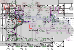
Figure 2: Illustration for the proof of Lemma 1.

One can argue $(\star)$ that inside any embedding-preserving visibility representation $\Gamma$ of $G_{h,\ell}$, there exists a copy of $H_{h,\ell}$ whose drawing $\Gamma_{H}$ satisfies (up to symmetry) the premise of the following claim.

Claim.

Let $\Gamma_{H}$ be an embedding-preserving visibility representation of $H_{h,\ell}$ such that all edges at box $P(v_{0})$ go downward, with edge $(v_{0},a_{1})$ leftmost among them. Assume that all boxes of $\Gamma_{H}$ intersect at most $h$ rows. Then $\Gamma_{H}$ uses at least $\ell+1$ rows and $P(v_{0})$ has width at least $4\ell+1$.

Proof.

We proceed by induction on $\ell$. In the base case ($\ell=1$) we have five vertical downward edges at $v_{0}$; this means that the height is at least 2 and $P(v_{0})$ must have width at least 5 as required.

Now assume $\ell\geq 2$ and study the five downward edges from $v_{0}$ to $a_{1},b_{1},v_{1},c_{1},\allowbreak d_{1}$, see also Fig. 2. The vertical edges $(v_{0},b_{1})$ and $(v_{0},d_{1})$ are crossed by edges $(a_{1},v_{1})$ and $(v_{1},c_{1})$, which means that the latter two edges must be horizontal. Since $(v_{0},a_{1})$ is leftmost, and the embedding is preserved, edge $(a_{1},v_{1})$ attaches on the left side of $P(v_{1})$ while $(v_{1},c_{1})$ attaches on the right side.

The counter-clockwise order of edges at $v_{1}$ contains $h-1$ edges (to $b_{1}$ and leaves) between $a_{1}$ and $a_{2}$. Since $P(v_{1})$ intersects at most $h$ rows, and $(v_{1},a_{1})$ attaches on its left side, therefore $(v_{1},a_{2})$ can not attach on its left side. Likewise $(v_{1},c_{2})$ can not attach on the right side of $P(v_{1})$. To preserve the embedding, therefore the edges from $v_{1}$ to the rest of $H_{h,\ell}$ must be drawn downward from $P(v_{1})$, with $(v_{1},a_{2})$ leftmost. Also observe that $H_{h,\ell}\setminus\{v_{0},a_{1},b_{1},c_{1},d_{1}\}$ contains a copy of $H_{h,{\ell-1}}$. Applying induction, there are at least $\ell$ rows below $P(v_{1})$, and $P(v_{1})$ has width at least $4\ell-3$. Adding at least one row for $P(v_{0})$, and observing that $P(v_{0})$ must be at least four units wider than $P(v_{1})$ proves the claim. ∎

So the claim holds, and $\Gamma_{H}$ (and with it $\Gamma$) has width and height $\Omega(\ell)$. ∎

As a consequence, we obtain two lower bound for visibility representation.

Theorem 3.1.

For any $N$ there is an $n$-vertex outer-1-plane graph with $n\geq N$ such that any embedding-preserving visibility representation has area $\Omega(n^{1.5})$.

Theorem 3.2.

For any $N$ there is an $n$-vertex outer-1-plane graph with $n\geq N$ such that any embedding-preserving bar visibility representation has area $\Omega(n^{2})$.

Roughly speaking, Theorem 3.1 uses $G_{\sqrt{N},\sqrt{N}}$, with leaves added to have maximum degree $\Theta(n)$, while Theorem 3.2 uses $G_{1,N}$. $(\star)$. The bounds then hold by Lemma 1 and Obs. 2.

4 Optimal Area Drawings

In this section we show how to compute an embedding-preserving visibility representation of area $O(n^{1.5})$ which is tight by Thm. 3.1. By Obs. 1 it suffices to construct a drawing of height $O(\sqrt{n})$.

Our construction is quite lengthy, so we mostly sketch it here via figures. We assume that $G$ is maximal-planar and a reference-edge $(s,t)$ on the outer-face of $G$ is fixed, and first choose a path $\pi$ in dual tree ${\overline{G^{*}}}$ (rooted at the face incident to $(s,t)$). Let $F\in\Theta(n)$ be the size of ${\overline{G^{*}}}$ (hence the number of inner faces of ${\overline{G}}$). As shown by Chan for binary trees [20] and generalized by us to arbitrary trees [13], $\pi$ can be chosen such that $\alpha^{p}+\beta^{p}\leq(1-\delta)F^{p}$, where $\alpha$ [$\beta$] is the maximum size of a left [right] subtree of $\pi$, $p=0.48$ and $\delta>0$ is a constant. Define a recursive function $h(F)=\max_{\alpha,\beta}\{h(\alpha)+h(\beta)\}+O(\sqrt{F})$ (with appropriate constants and base cases). Here the maximum is over all choices of $\alpha,\beta$ that satisfy the inequality. We construct a drawing of height $h(F)$.

So we first discuss how to draw the outer-1-path $P_{\pi}$ whose inner dual is $\pi$, plus all its hanging subgraphs (i.e., maximum subgraphs in $G\setminus P_{\pi}$). To do so, first create a visibility representation of $P_{\pi}$ on 5 rows such that edges with attached hanging subgraphs are drawn horizontally in the top or bottom row (see Fig. 3). Assume that each hanging subgraph $H$ has a $TC_{\sigma,\tau}$-drawing (for $\{\sigma,\tau\}=\{1,2\}$), i.e., a drawing where the endpoints of the reference-edge occupy the $T$op $C$orners and have height $\sigma$ and $\tau$. Then we can easily merge all hanging subgraphs, after expanding some boxes of $P_{\pi}$ one row outward. The resulting drawing has height $h(\alpha)+h(\beta)+O(1)$ since all hanging subgraphs below [above] correspond to left [right] subtrees of $\pi$.

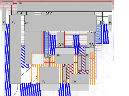
Figure 3: Drawing an outer-1-path (dark gray) and merging hanging subgraphs (blue striped) after expanding some vertex-boxes (light gray).

Alas, this path-drawing is not a $TC_{\sigma,\tau}$-drawing as required for the recursion. So we change the approach and first draw a larger subgraph that includes $P_{\pi}$. First extract the cap $C_{1}$, consisting of all neighbours of $s$ and $t$, see Fig. 4. This is an outer-1-path, so we can use a path-drawing and get a $TC_{\sigma,\tau}$-drawing of the cap (see the corresponding part in Fig. 5). The part of $P_{\pi}$ not in $C_{1}$ could be drawn as for outer-1-paths, but instead we first extract another cap $C_{2}$ at the edge common to $C_{1}$ and the rest of $P_{\pi}$. We draw $C_{2}$ as a path and place it (after suitable expansion of the vertices of $C_{1}$) below the drawing of $C_{1}$. This repeats $k$ times for some parameter $k$ of our choice ($k=2$ in the example). Then we draw the rest of $P_{\pi}$ (which we call handle) as a path.

A major difficulty is combining the drawing of the caps with the handle-drawing. Let $(x_{i},y_{j})$ be the edge common to caps and handle. It is not too difficult to change the boxes of $x_{i}$ and $y_{j}$ to combine the two boxes that represented them in the two drawings, see also Fig. 5. The main challenge is that for the two hanging subgraphs incident to $y_{j}$, there is no suitable place to merge a $TC_{\sigma,\tau}$-drawing. To resolve this, we split these hanging subgraphs further, and can then merge all their parts after adding $d(y_{j})$ more rows, where $d(y_{j})$ is the number of edges that $y_{j}$ has in these subgraphs (Fig. 6).

So the goal is to choose the parameter $k$ such that $d(y_{j})$ is small, because we need $d(y_{j})$ additional rows beyond the $h(\alpha)+h(\beta)$ that we budget for hanging subgraphs. Each extra cap also requires $O(1)$ additional rows but changes which vertex will take on the role of $y_{j}$. Crucially, the vertices $Y_{1},\dots,Y_{k}$ that take on the role of $y_{j}$ have disjoint edge sets that count for $d(\cdot)$. Since there are $O(n)$ edges in total, there exists a $k\in O(\sqrt{n})$ such that $d(Y_{k})\in O(\sqrt{n})$. With this choice of $k$, the recursive formula for the height hence becomes $h(\alpha)+h(\beta)+O(\sqrt{n})$, which by $F\in\Theta(n)$ and $\alpha^{p}+\beta^{p}\leq(1-\delta)n^{p}$ resolves to $O(\sqrt{n})$. $(\star)$

Figure 4: Our running example.

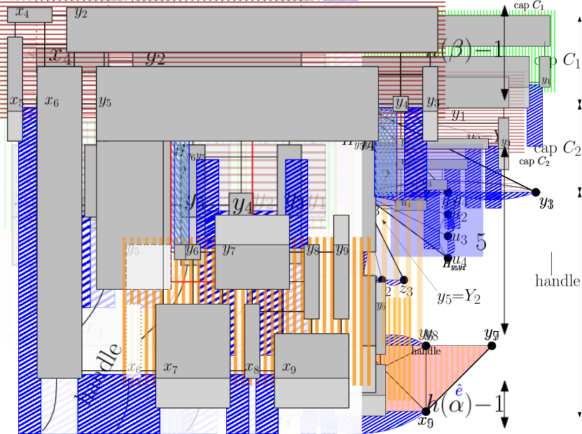
Figure 5: Drawing the complete example except for two hanging subgraphs $H_{y_{j}y_{j+1}}$ and $H_{y_{j-1}y_{j}}$. Here $j=5$.

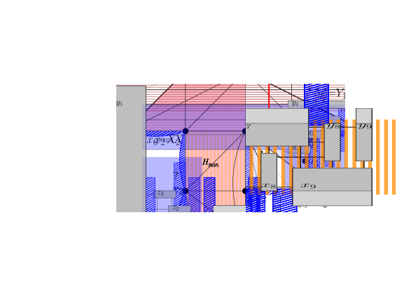
Figure 6: Closeup on breaking up and merging $H_{y_{j}y_{j+1}}$ and $H_{y_{j}y_{j-1}}$.

Theorem 4.1.

Every $n$-vertex outer-1-plane graph has an embedding-preserving visibility representation of area $O(n^{1.5})$, which is worst-case optimal.

5 Breaking the $\sqrt{n}$-barrier

We know that the height-bound of Theorem 4.1 is asymptotically tight due to Theorem 3.1. But the lower bound only holds for embedding-preserving visibility representations—can we get better height-bounds if we relax this restriction?

Theorem 5.1.

Any outer-1-planar graph $G$ has

• an embedding-preserving OPVR of complexity 1, and

• an embedding-preserving 1-bend orthogonal box-drawing, and

• a visibility representation that is not necessarily embedding-preserving and has at most one crossing per edge,

and the drawings have area $O(n^{1.48})$.

We again give the proof mostly in figures. $(\star)$ We assume as in Section 4 that the graph is planar-maximal, a reference-edge $(s,t)$ is given, and we construct a $TC_{\sigma,\tau}$-drawing for any given $\{\sigma,\tau\}=\{1,2\}$. We use $k=1$, i.e., we draw one cap and use the rest of $P_{\pi}$ as handle. Recall that the main difficulty in Section 4 was that two hanging subgraphs could not be merged using $TC_{\sigma,\tau}$-drawings since no suitable space was available.

If we change the drawing model (using a $\Gamma$-shape or a box in the cap-drawing for $y_{j}$) then one of these hanging subgraphs can use a $TC_{\sigma,\tau}$-drawing, and all edges can still be drawn, perhaps after adding a bend or changing the embedding. See Fig. 7. The other hanging subgraph uses a new drawing-type (i.e., different restrictions on shapes and locations of the endpoints of the reference-edge). It is not obvious that this exists, but we can show that it can be constructed by adding two rows. With this, the recursion for the height-function becomes $h(\alpha)+h(\beta)+O(1)$, which resolves to $O(n^{0.48})$ [20].

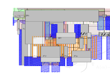
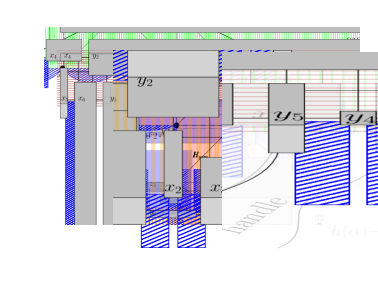
Figure 7: Inserting the two remaining hanging subgraphs when permitting ortho-polygons, or bends in edges, or after changing the embedding.

6 Optimum-height drawings in other drawing models

In this section we give drawings whose height (and area) is also optimal, but they are in a different drawing model (hence different lower bounds apply).

6.1 Embedding-preserving bar visibility representations

We proved in Theorem 3.2 that any embedding-preserving bar-visibility-representation has height $\Omega(n)$ for some outer-1-plane graphs. A fairly straight-forward greedy-construction shows that we can match this. The main difficulty is showing that such a drawing exists as all; the area-bound then follows from Obs. 1). $(\star)$

Theorem 6.1.

Any outer-1-planar graph $G$ has an embedding-preserving bar-visibility representation of area $O(n^{2})$ which is worst-case optimal.

6.2 More lower bounds

We now prove other lower bounds on the height that depend on the pathwidth $pw(G)$ and the number of crossings $\chi(G)$ of the outer-1-plane graph.

We recall that a path decomposition of a graph $G$ consists of a collection $B_{1},\dots,B_{\xi}$ of vertex-sets (“bags”) such that every vertex belongs to a consecutive set of bags, and for every edge $(u,v)$ at least one bag contains both $u$ and $v$. The width of such a path decomposition is $\max_{i}\{|B_{i}|-1\}$, and the pathwidth $pw(G)$ is the minimum width of a path decomposition of $G$. Any outer-1-planar graph has pathwidth $O(\log n)$, since it has treewidth 3 [3].

For planar drawings, the width and height of a drawing is lower-bounded by the pathwidth of the graph [31].

Less is known for non-planar drawings. It follows from the proof of Corollary 3 in [9] that any bar-1-visibility representation of graph $G$ has height at least $pw(G)+1$. Roughly speaking, we can extract a path decomposition of $G$ by scanning left-to-right with a vertical line and attaching a new bag whenever the set of intersected vertices changes. We use the same proof-idea here to show a lower bound for all OP-$\infty$-drawings. $(\star)$

Theorem 6.2.

Any OP-$\infty$-drawing of a graph $G$ (not necessarily outer-1-planar) has height and width $\Omega(pw(G))$.

By the remark after Obs. 2 hence some outer-1-planar graphs require area $\Omega(n\,pw(G))$ in all OP-$\infty$-orthogonal drawings.

If we specifically look at drawings that have no crossings, then we can also create a lower bound based on the number of crossings. This is easily obtained by modifying the lower-bound example from [7]. $(\star)$

Theorem 6.3.

For any $k$ and $n\geq 4k$, there exists an outer-1-plane graph with $n$ vertices and $k$ crossings that requires at least $2k$ height and width in any planar drawing.

In particular, the lower bound on the height of a planar OP-$\infty$-orthogonal drawing of $G$ is $\Omega(\max\{\allowbreak pw(G),\allowbreak\chi(G)\})$, which is the same as $\Omega(pw(G)+\chi(G))$.

6.3 More constructions

We now turn towards creating bar representations that prove that Theorem 6.2 and 6.3 are tight.

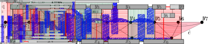
(a)

(b)

(c)

(d)

Figure 8: (a) Example-graph. (b) Drawing its skeleton and merging hanging subgraphs inward. Some vertex-boxes are artificially wide to match (c). (c) The bar-1-visibility representation obtained by moving some bars and sometimes traversing bars. (d) The planar bar-visibility representation obtained by moving some bars and extending them rightwards. Arrows indicate vertices that get moved outward beyond their neighbour on the right.

Theorem 6.4.

Every outer-1-plane graph $G$ has a planar bar visibility representation of area $O((pw(G){+}\chi(G))n)$ and a bar-1-visibility representation of area $O(n{\cdot}pw(G))$.

We can again only sketch the proof $(\star)$. We first draw the planar skeleton of some outer-1-path and the hanging subgraphs much as was done for outer-planar graphs in [5]. Based on the pathwidth (or actually the closely related parameter rooted pathwidth), extract a root-to-leaf path $\pi$ in the dual tree ${\overline{G^{*}}}$ such that the rooted pathwidth of all subtrees is smaller. Expand $P_{\pi}$ by adding all neighbours of $s$ to get $P_{\pi}^{+}$. Create a bar visibility representation of ${\overline{P_{\pi}^{+}}}$ on three rows. See Fig. 8(b). Now merge hanging subgraphs “inward”, i.e., inside the faces of ${\overline{P_{\pi}}}$. They hence share rows and the height is only $O(1)$ more than the one of the subgraphs and works out to $O(pw(G))$. For the merging we need $TC_{1,1}$-drawings, but with our placement of $(s,t)$ this can easily be achieved.

However, we have not yet drawn the crossings in $P_{\pi}^{+}$. One of each pair of crossing edges can be realized inside a face of ${\overline{P_{\pi}^{+}}}$. For bar-1-visibility representations, we realize the other edges by moving vertex-bars inward or outward by one unit (plus some special handling near $s$ and $t$). After suitable lengthening of bars the other edge in a crossing can then be realized, sometimes by traversing a bar. See Fig. 8(c). For planar drawings, we move bars outward sufficiently far (proportionally to the number of crossings on the right) such that they can be extended rightward without intersecting other elements of the drawing. The other edge in a crossing can then be drawn on the right. See Fig. 8(d).

7 Conclusions and open problems

In this paper, we studied visibility representations of outer-1-planar graphs. We showed that if the embedding must be respected, then $\Omega(n^{1.5})$ area is sometimes required, and $O(n^{1.5})$ area can always be achieved. We also studied numerous other drawing models, showing that $o(n^{1.5})$ area can be achieved as soon as we allow bends in the vertices or the edges or can change the embedding. We also achieve optimal area for bar-1-visibility representations and planar visibility representations. Following the steps of our proofs, it is clear that the drawings can be constructed in polynomial time; with more care when handing subgraph-drawings (and observing that path $\pi$ can be found in linear time [13, 8]) the run-time can be reduced to linear. A number of open problems remain:

• Our drawings of height $O(n^{0.48})$ were based on the idea of so-called LR-drawings of trees [20], which in turn were crucial ingredients for obtaining small embedding-preserving straight-line drawings of outer-planar graphs. With a different approach, Frati et al. [33] achieved height $O(n^{\varepsilon})$ for drawing outer-planar graphs. Can we achieve height $O(n^{\varepsilon})$ (hence area $O(n^{1+\varepsilon})$ in some of our constructions as well?

• Our bar-1-visibility representations do not preserve the embedding, both because the edges that go through some vertex-bar are not in the right place in the rotation, and because we merge hanging subgraphs inward. What area can we achieve if we require the embedding to be preserved?

• We achieved height $O(n^{0.48})$ in complexity-1 OPVRs. It is not hard to achieve the optimal height $O(pw(G))$ if we allow higher complexity (complexity 4 is enough; we leave the details to the reader). What is the status for complexity 2 or 3, can we achieve height $o(n^{0.48})$?

Finally, are there other significant subclasses of 1-planar graphs for which we can achieve $o(n^{2})$-area drawings, either straight-line or visibility representations?

Appendix 0.A Missing details from Section 2

Observation 3.

Let $\Gamma$ be an OP-$\infty$-orthogonal drawing with constant vertex and bend complexity. Then we may assume that the width and height is $O(n+m)$.

Proof.

Due to the restrictions on the complexity/bends, we have $O(n{+}m)$ segments in edge-polylines or vertex-polygons. Since all segments are horizontal and vertical, we can delete empty rows/columns and so need at most one row [column] per horizontal [vertical] segment (and often less). ∎

Observation 4.

Let $\Gamma$ be an OP-$\infty$-orthogonal drawing with constant vertex complexity in a $W\times H$-grid. Then $\max\{W,H\}\in\Omega(\text{maximum degree of $G$})$.

Proof.

After rotation we may assume that $W\geq H$. Let $v$ be the vertex with maximum degree $\Delta$, and let $k\in O(1)$ be the complexity of polygon $P(v)$. If $W\geq\Delta/(8k+8)\in\Omega(\Delta)$ then we are done, so assume not. Consider a horizontal segment $s$ of polygon $P(v)$. This intersects at most $\Delta/(8k+8)$ columns, hence at most $\Delta/(4k+4)$ edges can end vertically at $s$. (This bound could actually be improved to $\Delta/(2k+2)$, but this makes no difference asymptotically.) Polygon $P(v)$ has $2k+2$ horizontal segments, so at most $(2k+2)\cdot\Delta/(4k+4)=\Delta/2$ edges can end vertically at $P(v)$. So there are at least $\deg(v)-\Delta/2=\Delta/2$ edges that attach horizontally at $P(v)$. Since $P(v)$ has $2k+2$ horizontal edges, at least one of them hence has length $\Delta/(8k+8)$ or more. Therefore $H\geq\Delta/(8k+8)>W$, a contradiction. ∎

Appendix 0.B Missing details from Section 3

Missing part of the proof of Lemma 1:

Fix an arbitrary embedding-preserving visibility representation $\Gamma$ of $G_{h,\ell}$ where all vertex-boxes intersect at most $h$ rows. Consider one copy $H$ of $H_{h,\ell}$ and the box $P(v_{0})$ of $v_{0}$. We say that $H$ is right of $v_{0}$ if some part of the right side of $P(v_{0})$ belongs to the interior of the induced drawing of $H$. Since $P(v_{0})$ intersects at most $h$ rows, there are at most $h$ edges that attach horizontally at the right side of $P(v_{0})$. If $H$ is right of $v_{0}$, then these attachment points are entirely used up by edges from $v_{0}$ into $H$ and/or edges from $v_{0}$ to leaves that come before and after $H$ at $v_{0}$. (There are $h-1$ leaves on each side of $H$, which uses up all such points since the embedding is respected.)

So at most one copy of $H_{h,\ell}$ is right of $v_{0}$, and symmetrically at most one copy of $H_{h,\ell}$ is left of $v_{0}$. So there exists a copy $H$ of $H_{h,\ell}$ that is neither left nor right of $v_{0}$, and so the interior of the induced drawing of $H$ uses only the top side of $P(v)$ or only the bottom side of $P(v)$. Up to symmetry, we may hence assume that all edges from $v_{0}$ to $H$ go downward from $v_{0}$. Since the drawing respects the embedding, edge $(v_{0},a_{1})$ must be the leftmost among the edges from $v_{0}$ into $H$.

Theorem 3.1.

For any $N$ there is an $n$-vertex outer-1-plane graph with $n\geq N$ such that any embedding-preserving visibility representation has area $\Omega(n^{1.5})$.

Proof.

Set $h=\ell=\lceil\sqrt{N}\rceil$ and define graph $G$ to be of $G_{h,\ell}$ with $\ell^{2}$ further leaves added at $v_{0}$ (at arbitrary places); this has $n=\Theta(h\ell)=\Theta(N)$ vertices. Fix an arbitrary embedding-preserving visibility representation of $G$ in a $W\times H$-grid. Up to symmetry, assume $W\geq H$. By Obs. 2 we have $W\geq\deg(v_{0})\geq\ell^{2}\in\Omega(n)$. If any vertex-box has height more than $h$, then this alone requires $H\geq h=\ell\in\Omega(\sqrt{n})$ and we are done. If all vertex-boxes have height at most $h$, then by Lemma 1 the height is $\Omega(\ell)=\Omega(\sqrt{n})$, and again we are done. ∎

inline]TB: It would be nice to work out the exact constant in the $\Omega$, at least for some values of $N$. I wouldn’t put the proof itself here, but some sentence such as “One can show that with a more careful choice of $h,\ell$ the lower bound is actually $cn^{1.5}$.” (where $c$ gets replaced by whatever). I think $c$ is not too too small (maybe around $\tfrac{1}{25}$?), so this lower bound is not as useless as others.

Theorem 3.2.

For any $N$ there is an $n$-vertex outer-1-plane graph with $n\geq N$ such that any embedding-preserving bar visibility representation has area $\Omega(n^{2})$.

Proof.

Set $h=1$ and $\ell=N$ and apply Lemma 1 to $G_{h,\ell}$. This graph has $\Theta(\ell)=\Theta(N)$ vertices and requires width and height $\Omega(\ell)=\Omega(n)$ in any embedding-preserving visibility representation where boxes intersect only one row. ∎

Figure 9 shows drawings of the lower-bound graph with linear area in other drawing-models.

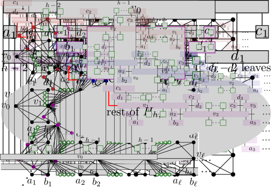
Figure 9: Drawings of $G_{h,l}$ with constant height, from top to bottom: an embedding-preserving ortho-polygon visibility representation with vertex complexity $1$, a bar-visibility representation for a changed embedding (see the red edges), an embedding-preserving bar-1-visibility representation, and an embedding-preserving 1-bend orthogonal box-drawing (the red edges have a bend).

Appendix 0.C Missing details from Section 4

0.C.1 Preliminaries

We first need a few definitions and assumptions which will also be used in Section 5 and 6. We shall assume without loss of generality that the input graph is plane-maximal: If not, we can always augment it with dummy edges which will be removed at the end of the construction.

Let $G$ be a plane-maximal outer-$1$-plane graph. We assume throughout that a reference-edge $(s,t)$ has been fixed, which is an edge on the outer-face, with $s$ before $t$ in the clockwise order of vertices along the outer-face. Recall that ${\overline{G^{*}}}$ denotes the inner dual of the planar skeleton of $G$; we consider ${\overline{G^{*}}}$ to be rooted at the face $f_{st}$ of ${\overline{G}}$ that is incident to $(s,t)$. A root-to-leaf path $\pi$ in ${\overline{G^{*}}}$ is a path that begins at $f_{st}$ and ends at a leaf of ${\overline{G^{*}}}$. Any maximal subtree of ${\overline{G^{*}}}\setminus V(\pi)$ is a rooted subtree that can be classified as left or right subtree depending on whether its root is left or right of the path-child at its parent in $\pi$.

The $\pi$-path $P_{\pi}$ of $G$ is the plane-maximal outer-1-path $P_{\pi}$ whose inner dual is $\pi$. Since $\pi$ is a root-to-leaf path, $P_{\pi}$ contains $(s,t)$ on its outer-face, and we can pick one outer-face edge $\hat{e}\neq(s,t)$ at the face of ${\overline{P_{i}}}$ corresponding to the leaf of $\pi$. We call these the end-edges of $P_{\pi}$.

As outlined, we create our drawings by first drawing a subgraph $U$ that contains all of $P_{\pi}$ and then merging the rest. Enumerate the outer-face of $U$ in counter-clockwise direction as $s{=}x_{0},x_{1},\dots,x_{\ell},y_{r},y_{r-1},\dots,y_{0}{=}t$, where $(x_{\ell},y_{r})$ is the end-edge $\hat{e}$ of $P_{\pi}$. (See e.g. Fig. 12(a).) We call $\langle x_{0},x_{1},\dots,x_{\ell}\rangle$ and $\langle y_{0},y_{1},\dots,y_{r}\rangle$ the left and right boundaries (with respect to the end-edges). For $0\leq j<r$, edge $(y_{j},y_{j+1})$ is on the outer-face of $U$, but need not be on the outer-face of $G$. If it is not, then define the hanging subgraph $H_{y_{j}y_{j+1}}$ of $U$ to be the subgraph induced by the vertices along the path on the outer-face between $y_{j}$ and $y_{j+1}$ that excludes $(s,t)$. Since $U$ includes $P_{\pi}$, the inner dual of $H_{y_{i}y_{j+1}}$ is part of a right subtree of $\pi$; correspondingly we call $H_{y_{j}y_{j+1}}$ a right hanging subgraph. The left hanging subgraph $H_{x_{i}x_{i+1}}$ (for $0\leq i<\ell$) is defined symmetrically.

0.C.2 Path $\pi$, function $h$ and drawing-types

We want a root-to-leaf path $\pi$ in ${\overline{G^{*}}}$ for which the sizes of the left and right subtrees are balanced in some sense. Chan [20] proved the existence of such paths for binary trees, and we recently generalized this to arbitrary rooted trees:

Lemma 2 ([13]).

Let $p=0.48$. Given any rooted tree $T$ of $n$ vertices, there exists a root-to-leaf path $\pi$ such that for any left subtree $\alpha$ and any right subtree $\beta$ of $\pi$, $|\alpha|^{p}+|\beta|^{p}\leq(1-\delta)n^{p}$ for some constant $\delta>0$.

Fix this path $\pi$ for the rest of this section. Slightly abusing notation, we now use $\alpha$ and $\beta$ for the size of the maximum left/right subtree of $\pi$ in ${\overline{G^{*}}}$ (rather than the trees themselves). Going over to graph $G$, we will measure its size by the number $F$ of inner faces in ${\overline{G}}$. Then $\alpha$ and $\beta$ are the maximum size of a left/right hanging subgraph of $P_{\pi}$. Since we draw a super-graph $U$ of $P_{\pi}$, $\alpha$ and $\beta$ are upper bounds on the size of a left/right hanging subgraph of $U$.

Let $h(F)$ be the recursive function that satisfies $h(1)=3$ and

$$h(F)=\max_{\alpha^{p}+\beta^{p}\leq(1-\delta)F^{p}}h(\alpha)+h(\beta)+11\sqrt{F}+7$$

for $F>1$, where $p=0.48$ and $\delta>0$ are as in Lemma 2. One can easily show that $h(F)\leq c\sqrt{F}-7$, where $c=\max\{10,12/\delta\}$. It hence suffices to find drawings of height $h(\alpha)+h(\beta)+11\sqrt{F}+7$ to obtain drawings of height $O(\sqrt{F})=O(\sqrt{n})$ (observe that $F\in\Theta(n)$).

As outlined, we restrict drawings of hanging subgraphs as follows. For integers $\sigma,\tau$, let a $(\sigma,\tau)$-Top-Corner drawing ($TC_{\sigma,\tau}$-drawing for short) be a drawing of $G$ where $s$ and $t$ occupy the top corners, and the boxes of $s$ and $t$ have height $\sigma$ and $\tau$, respectively. See Fig. 10.

For later merging-steps, we briefly mention here that these drawings can be modified to satisfy other properties. Assume we have a $TC_{2,1}$-drawing. Since $(s,t)$ is an edge, it must necessarily be drawn horizontally between the boxes of $s$ and $t$. Since the box of $t$ has height 1, no other vertex occupies the top row. Without changing the height, we can therefore change $t$ into a bar that spans the entire top row and retract $s$ to be a bar on the left end of the second row; see Fig. 10. We call the result a $(2,1)$-Top-Bar drawing ($TB_{2,1}$-drawing for short). We can also transform the drawing into a $TC_{\sigma,\tau}$-drawing, for any $\tau\geq 1$ and $\sigma\geq\tau+1$, by inserting $\tau-1$ and $\sigma-\tau-1$ rows above and below the top row, respectively, and extending the vertex-boxes. Similar transformations can be applied to a $TC_{1,2}$-drawing.

With this, we can state our overall goal:

Figure 10: Drawing-types (the rightmost two are needed in Section 5).

Lemma 3.

Let $G$ be an outer-1-plane graph with reference-edge $(s,t)$. Then for any $\{\sigma,\tau\}\in\{1,2\}$, $G$ has an embedding-preserving visibility representation that is a $TC_{\sigma,\tau}$-drawing with height at most $h(F)$.

The proof of this lemma is by induction on $F$. Since $G$ is plane-maximal, if $F=1$ then $G$ is either a triangle or a $K_{4}$ drawn with one crossing. Either way we can easily find a $TC_{\sigma,\tau}$-drawing of height at most $3=h(1)$. The remainder of this section will prove the induction step. Fix $\pi,\alpha,\beta$ as explained above.

0.C.3 Drawing a path.

As a first step, we will give a simple construction that unfortunately does not place $s,t$ where we need them, but places them on the left side instead.

Lemma 4.

Fix $\{\sigma^{\prime},\tau^{\prime}\}=\{2,3\}$. $G$ has an embedding-preserving visibility representation $\Gamma$ of height $h(\alpha)+h(\beta)+3$. Furthermore, $P(s)$ and $P(t)$ have height $\sigma^{\prime}$ and $\tau^{\prime}$, respectively, both abut the left side of the bounding box, and there are $h(\alpha)-1$ rows below $P(s)$ and $h(\beta)-1$ rows above $P(t)$.

Figure 11: Drawing an outer-1-path (dark gray) and merging hanging subgraphs (blue striped).

Proof.

We first draw $P_{\pi}$ on five rows (see the orange hatched part of Fig. 11) and then merge the hanging subgraphs.

Assume the outer-face of $P_{\pi}$ is enumerated as $x_{0},\dots,x_{\ell},y_{r},\dots,y_{0}$ as before. The boxes of $x_{0},\dots,x_{\ell}$ all intersect row 1 (of our five rows), in this order from left-to-right, while the boxes of $y_{0},\dots,y_{r}$ all intersect row 5. The outer-face edges along these paths can hence be realized horizontally. All vertex-boxes have height 1, 2 or 3, and we determine this (as well as their $y$-coordinates) by parsing the faces $f_{1},\dots,f_{k}$ of ${\overline{P_{\pi}}}$, beginning at $f_{st}$, and extending the drawing rightwards. The heights of $x_{0}{=}s$ and $y_{0}{=}t$ are determined by $\sigma^{\prime}$ and $\tau^{\prime}$. Assume we have drawn everything up to some face $f_{h-1}$, which ends at edge $(x_{i},y_{j})$. Boxes $P(x_{i}),P(y_{j})$ are partially drawn and their heights are $\{2,3\}$ (but we do not know which one has which height). The next face $f_{h}$ can have one of five configurations:

• $f_{h}$ has no crossing (hence it is a triangle). One of $\{x_{i},y_{j}\}$ also belongs to $f_{h+1}$ (or is in $\{x_{\ell},y_{r}\}$ if $h=k$). Let us assume that this is $y_{j}$, the other case is symmetric. See e.g. $\{x_{0},x_{1},y_{0}\}$ in Fig. 11. In this case, $P(x_{i})$ ends, $P(x_{i+1})$ begins (with the same height as $P(x_{i})$) and $P(y_{j})$ extends further rightwards. Edge $(x_{i+1},y_{j})$ can be inserted vertically.

• $f_{h}$ has a crossing and neither $x_{i}$ nor $y_{j}$ belongs to $f_{h+1}$ (or is in $\{x_{\ell},y_{r}\}$ if $h=k$). See e.g. $\{x_{3},x_{4},y_{2},y_{3}\}$. We call such a crossing an opposite-boundary crossing since both crossing edges connect opposite boundaries. Let us assume that $P(x_{i})$ has height 3 and $P(y_{j})$ has height 2; the other case is symmetric. In this case, $P(x_{i})$ ends and $P(x_{i+1})$ begins with height 2, which means that we can draw $(x_{i+1},y_{j})$ vertically. Then $P(y_{j})$ ends and $P(y_{j+1})$ begins with height 3, which means that we can draw $(x_{i},y_{j+1})$ horizontally along row 3.

• $f_{h}$ has a crossing and one of $\{x_{i},y_{j}\}$ belongs to $f_{h+1}$ (or is in $\{x_{\ell},y_{r}\}$ if $h=k$). Let us assume that this is $x_{i}$, the other case is symmetric. See e.g. $\{x_{1},y_{0},y_{1},y_{2}\}$. We call such a crossing a same-boundary crossing since one of the crossing edges connects two vertices on the same boundary. In this case, $P(y_{j})$ ends and $P(y_{j+1})$ begins (with height one less than the height of $P(y_{j})$), which means that we can draw $(y_{j+1},x_{i})$ vertically. Then $P(y_{j+1})$ ends and $P(y_{j+2})$ begins (with the same height as $P(y_{j})$), which means that we can draw $(y_{j},y_{j+2})$ horizontally along the bottom row of $P(y_{j})$ and $P(y_{j+2})$.

Extending the drawing one face at a time gives us an embedding-preserving visibility representation $\Gamma_{P}$ of $P_{\pi}$. Before merging hanging subgraphs, we first parse along the top and bottom row from left to right and extend every second box by one row “outward” (i.e., away from $\Gamma_{P}$). Consider a left hanging subgraph $H_{x_{i}x_{i+1}}$. Edge $(x_{i},x_{i+1})$ is drawn horizontally along the bottom row of $\Gamma_{P}$. After the extension, one of $x_{i},x_{i+1}$ (say $x_{i}$) extends one row further down. This means that we can merge a (recursively obtained) $TC_{2,1}$-drawing $\Gamma_{H}$ of $H_{x_{i}x_{i+1}}$ in the rows below $(x_{i},x_{i+1})$. This requires at most $h(\alpha)-1$ rows below the rows for $P_{\pi}$ since $\Gamma_{H}$ has height at most $h(\alpha)$ and the row for edge $(x_{i},x_{i+1})$ can be used by both $\Gamma_{P}$ and $\Gamma_{H}$. Symmetrically we can merge right hanging subgraphs using up to $h(\beta)-1$ rows above $\Gamma_{P}$.∎

0.C.4 Drawing a cap

Define the cap $C$ to be the outer-1-path that contains $s,t$ and all vertices adjacent to $s$ or $t$, and let the umbrella [10] be the union of $C$ and $P_{\pi}$; we denote it by $U_{\pi}$. See also Fig. 12(a). We will later draw all of $U_{\pi}$, but for now are only concerned with drawing $C$. Enumerate the outer-face of $U_{\pi}$ as $x_{0}{=}s,\dots,x_{r},y_{\ell},\dots,y_{0}{=}t$. Assume that $P_{\pi}\subsetneq C$ (in the other case we only have to draw $C$, which will be easier). Of special interest is then the transition edge $(x_{i},y_{j})$, which is the edge on the outer-face of the cap that is an inner edge of $P_{\pi}$. Sometimes we use the notation $X:=x_{i}$ and $Y:=y_{j}$. The handle $P_{h}$ is the part of $P_{\pi}$ not in $C$; thus $P_{h}$ is the outer-1-path that contains all vertices of $P_{\pi}$ between $(X,Y)$ and end-edge $\hat{e}$. Note that the handle (plus its hanging subgraphs) can be viewed as the hanging subgraph $H_{XY}$ of the cap.

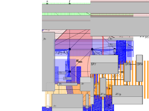
(a)

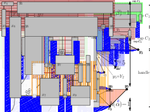
(b)

Figure 12: (a) An umbrella $U_{\pi}$. $P_{\pi}$ is shaded. (b) Our running example with its 2-cap umbrella $U^{(2)}$ and the hanging subgraphs $H_{y_{5}y_{4}}$ and $H_{y_{6}y_{5}}$ expanded. Fig. 11 was a drawing of its handle. inline]Time permitting, redraw this figure to have smaller horizontal spacing and perhaps a different layout at the “wings” so that we can make labels bigger.

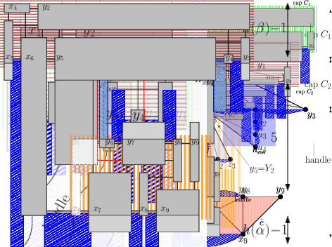
Figure 13: A $TC_{1,2}$-drawing of a cap, both when $f_{st}$ has a crossing and otherwise. The naming is consistent with the example from Fig. 12(b).

Lemma 5.

Let $C$ be the cap, and let $\{\sigma,\tau\}=\{1,2\}$. The subgraph formed by $C$ and its hanging subgraphs (except $H_{XY}$) has an embedding-preserving visibility representation of type $TC_{\sigma,\tau}$ and height $\max\{h(\alpha),h(\beta)\}+3$.

Proof.

The path-drawing from Lemma 4 satisfies this, as long as we re-define the path that we use and modify boxes a bit. Note the cap can be viewed as $P_{\pi^{\prime}}$ for the path $\pi^{\prime}$ that begins at the inner face of ${\overline{G}}$ incident to $(x_{1},s)$ and ends at the inner face of ${\overline{G}}$ incident to $(t,y_{1})$. Choose $\tau^{\prime}$ as follows: If $f_{st}$ has a crossing, then set $\tau^{\prime}=\sigma+1$, otherwise set $\tau^{\prime}=3$. Apply Lemma 4 with respect to this path $\pi^{\prime}$, reference-edge $(x_{1},s)$, and values $\tau^{\prime}$ and $\sigma^{\prime}=\{2,3\}\setminus\tau^{\prime}$hence $P(x_{1})$ has height $\sigma^{\prime}$ and $P(s)$ has height $\tau^{\prime}$. Since $(s,t)$ is on the outer-face, there are no hanging subgraphs to be merged above, and the top two rows of the drawing contain only $s$, $t$, and edge $(s,t)$, we can delete one of these rows. If $f_{st}$ had no crossing, then both $P(s)$ and $P(t)$ now have height 2; reduce the height of one of them to 1 (after extending vertical edges) as dictated by $\{\sigma,\tau\}$. If $f_{st}$ had a crossing, then $P(s)$ now has height $\sigma$ and the height of $P(t)$ is different from $P(s)$, hence $P(t)$ has height $\tau$. All other conditions are easily verified. ∎

0.C.5 Drawing an umbrella.

Now we need to combine the cap-drawing of Lemma 5 with the path-drawing of Lemma 4 (applied to the handle). This combination step is the most challenging part of our construction and illustrated in Fig. 14. Assume $\{\sigma,\tau\}=\{1,2\}$ has been given. We split the explanation of how to draw $G$ into two steps.

Step 1: Draw cap, handle, and most hanging subgraphs.

We have two subcases, depending on the configuration of $(x_{i},y_{j})$ in handle $P_{h}$. Let $f,f^{\prime}$ be the first two faces of ${\overline{P_{h}}}$, enumerated starting at transition edge $(x_{i},y_{j})$. Not both $x_{i}$ and $y_{j}$ can belong to $f^{\prime}$. We assume here that $x_{i}$ does not belong to $f^{\prime}$, the other case is symmetric (we would merge the handle in leftward direction).

Using Lemma 5, obtain a $TC_{\sigma,\tau}$-drawing $\Gamma^{+}_{C}$ of cap $C$ and its hanging subgraphs except $H_{XY}$. We remove the drawings of hanging subgraphs $H_{x_{i-1}x_{i}}$ and $H_{y_{j-1}y_{j}}$ from $\Gamma_{C}^{+}$; they will be handled later. Recall that as part of creating $\Gamma_{C}^{+}$ we expanded every second box of $x_{1},\dots,x_{i},y_{j},\dots,y_{1}$ downward by one unit; we assume here that the choice has been done such that $x_{i}$ is extended downward and $y_{j}$ is not.

Using Lemma 4, obtain a drawing $\Gamma_{P}^{+}$ of $P_{h}$ and its hanging subgraphs (i.e., graph $H_{XY}$), using $(x_{i},y_{j})$ as reference-edge and $\sigma^{\prime}=3$ so that $P(x_{i})$ has height 3. We use $\Gamma_{P}$ to denote the drawing of $P_{h}$ within $\Gamma_{P}^{+}$. Omit from $\Gamma_{P}^{+}$ the drawings of hanging subgraphs $H_{x_{i}x_{i+1}}$ and $H_{y_{j}y_{j+1}}$ for special handling later.

To merge the two drawings, insert sufficiently many new columns between $y_{j}$ and $y_{j-1}$ in $\Gamma_{C}^{+}$, and place $\Gamma_{P}^{+}$ sufficiently far below the horizontal line segment $(y_{j},y_{j-1})$. Here, “sufficiently far” means that there are at least $h(\beta)-1$ rows between $(y_{j},y_{j-1})$ and $\Gamma_{P}$; therefore the right hanging subgraphs of $P_{h}$ fit without overlapping $\Gamma_{C}^{+}$. (We will actually need even more rows later.)

We now let $P(y_{j})$ be the minimum box that includes both of boxes of $y_{j}$ in $\Gamma^{+}_{C}$ and $\Gamma^{+}_{P}$; with our placement of $\Gamma^{+}_{P}$ and because we removed hanging subgraphs this does not overlap other vertices. To unify the two copies of $x_{i}$, we need to be more careful. Expand the copy of $x_{i}$ in $\Gamma^{+}_{C}$ vertically downward until the rows containing the copy of $x_{i}$ in $\Gamma^{+}_{P}$; this is $P(x_{i})$. Delete the copy in $\Gamma^{+}_{P}$, and expand all its incident horizontal edges leftward until $P(x_{i})$. By case-assumption $x_{i}$ belongs only to the first face of $P_{h}$ and has height 3. One verifies that therefore (in $\Gamma_{P}^{+}$) all its incident vertically drawn edges are either $(x_{i},y_{j})$ (which we can ignore because it is also realized in $\Gamma^{+}_{C}$) or belong to the hanging subgraph $H_{x_{i}x_{i+1}}$ (whose drawing was omitted). So extending only horizontal edges suffices to draw all incident edges at $x_{i}$.

Figure 14: Drawing an umbrella. Two hanging subgraphs are not yet included.

We have four hanging subgraphs that were omitted. Two of them are easily merged as follows. For graph $H_{x_{i-1}x_{i}}$, use a $TC_{1,h}$-drawing, where $h\geq 2$ is the height of $P(x_{i})$; recall that we can create this from a $T_{1,2}$-drawing by inserting rows. For graph $H_{x_{i}x_{i+1}}$, the bottom sides of $P(x_{i})$ and $P(x_{i+1})$ are one row apart and so we can merge a $TC_{1,2}$-drawing almost as it would have been done in $\Gamma^{+}_{P}$ (the only change is that we stretch it horizontally so that it uses the new location of $P(x_{i})$).

Step 2: Drawing hanging subgraphs at $y_{j}$.

We still need to merge hanging subgraphs $H_{y_{j}y_{j-1}}$ and $H_{y_{j+1}y_{j}}$, and this causes major difficulties because the endpoints of their reference-edge are not in a position that we can match in a drawing of the subgraph. We solve this by breaking $H_{y_{j}y_{j-1}}$ and $H_{y_{j+11}y_{j}}$ down further, and using one extra row for each edge incident to $y_{j}$ in these subgraphs. Specifically, let $u_{1},\dots,u_{d}$ be neighbours of $y_{j}$ in $H_{y_{j}y_{j-1}}$ indexed in clockwise order, beginning with $y_{j-1}{=}u_{1}$. Insert $d$ new columns to the right of $\Gamma_{P}^{+}$ to widen $y_{j-1}$, and place $u_{2},\dots,u_{d}$ as left-aligned bars of length $d{-}1,\dots,1$ in the newly added columns and below $u_{1}$. We can connect them horizontally to $y_{j}$. For any edge $(u_{h},u_{h+2})$ that may exist, shorten the left end of $P(u_{h+1})$ by one unit so that a vertical visibility between $u_{h}$ and $u_{h+2}$ is formed. Assuming we left at least $d+h(\beta)-2$ rows between $(y_{j},y_{j-1})$ and $\Gamma_{P}$, we can now merge the hanging subgraphs $H_{u_{h}u_{h+1}}$ in the rows below the staircase formed by the bars, using an $TB_{2,1}$-drawing. Note that crucially there is no hanging subgraph at $(y_{j},u_{d})$, otherwise $y_{j}$ would have further neighbours in $H_{y_{j}y_{j-1}}$. So this merges all of $H_{y_{j}y_{j-1}}$ as required.

Similarly, to merge $H_{y_{i+1}y_{i}}$, let $z_{1},\dots,z_{d^{\prime}}$ be neighbours of $y_{j}$ in $H_{y_{j}y_{j+1}}$, indexed in counter-clockwise order, beginning at $y_{j+1}$. Place $z_{2},\dots,z_{d^{\prime}}$ as bars forming a staircase, in the $d^{\prime}{-}1$ rows above $y_{i+1}$. Shorten left ends if needed so that edges among them drawn. Merge hanging subgraph $H_{z_{h}z_{h+1}}$ (for $h=1,\dots,d^{\prime}-1$) in the rows above, and note that this merges all of $H_{y_{j+1}y_{j}}$ and creates no overlap as long as there are at least $d{-}1+d^{\prime}{-}1+h(\beta){-}1=d+d^{\prime}+h(\beta)-3$ rows between $(y_{j},y_{j-1})$ and $\Gamma_{P}$. See Fig. 15.

Figure 15: Closeup: Inserting the two remaining hanging subgraphs.

For any vertex $v$ in $U_{\pi}$, let $d(v)$ be the number of edges incident to $v$ that do not belong to $U_{\pi}$. The height of our construction depends on $d(y_{j})$ as follows.

Lemma 6.

For any $\{\sigma,\tau\}=\{1,2\}$, $G$ has an embedding-preserving visibility representation $\Gamma$ that is a $TC_{\sigma,\tau}$-drawing with height $h(\alpha)+h(\beta)+D+7$, where $D=\max\{d(x_{i}),d(y_{j})\}$ if the umbrella has transition edge $(x_{i},y_{j})$ and $D=0$ otherwise.

Proof.

This holds by Lemma 5 if there is no transition edge (and hence $H_{XY}$ is empty), so assume $(x_{i},y_{j})$ exists. The drawing construction was already given above, so we only need to analyze the height. The left hanging subgraphs use at most $h(\alpha){-}1$ rows below $\Gamma_{P}$. The right hanging subgraphs can be merged as long as we leave $d+d^{\prime}+h(\beta)-3$ rows between $(y_{j},y_{j-1})$ and $\Gamma_{P}$. By $d(y_{j})=d+d^{\prime}-2$ this equals $d(y_{j})+h(\beta)-1$ rows. Recall that we made an assumption on $y_{j}$; in the other symmetric case where we merge leftward we would use $x_{i}$ rather than $y_{j}$ here. Finally we need 9 rows for the boxes of the cap and the handle, and so the total height is as required. ∎

0.C.6 Drawing a $k$-cap umbrella.

If our graph has small maximum degree, then Lemma 6 gives us the required recursion and we are done. We now show that even for larger maximum degree we can achieve height $O(\sqrt{n})$ by extracting multiple caps before drawing the remaining part of $P_{\pi}$.

Roughly speaking, a $k$-cap umbrella consists of taking caps $k$ times (always along the path $\pi$) and using the rest as handle. Formally, let $C_{1}$ be the cap with respect to reference-edge $(s,t)$. If all of $P_{\pi}$ belongs to $C_{1}$ then the recursive procedure stops, $(X_{k},Y_{k})$ is undefined and $C_{2},\dots,C_{k}$ are the empty set. Otherwise, let $(X_{1},Y_{1})$ be the transition edge of $C_{1}$ and let $H_{1}$ be the hanging subgraph at $(X_{1},Y_{1})$. Repeat in $H_{1}$, i.e., let $C_{2}$ be the cap of $H_{1}$ (with respect to reference-edge $(X_{1},Y_{1})$), let $(X_{2},Y_{2})$ be its transition edge, let $H_{2}$ be the hanging subgraph at $(X_{2},Y_{2})$ etc., until we obtain cap $C_{k}$ and its transition edge $(X_{k},Y_{k})$. (If all of $P_{\pi}$ belongs to $C_{1}\cup\dots\cup C_{i}$ for some $i\leq k$ then $C_{i+1},\dots,C_{k}$ are empty sets and $(X_{k},Y_{k})$ is undefined.) The $k$-cap umbrella $U^{(k)}$ is then $C_{1}\cup\dots\cup C_{k}\cup P_{\pi}$, and its last transition edge is $(X_{k},Y_{k})$ (which may be undefined). See Fig. 12(b).

Lemma 7.

For any $\sigma,\tau=\{1,2\}$, and any $k\geq 1$, $G$ has an embedding-preserving visibility representation $\Gamma$ that is a $TC_{\sigma,\tau}$-drawing with height $h(\alpha)+h(\beta)+3k+D+4$, where $D=\max\{d(X_{k}),d(Y_{k})\}$ if the last transition edge is $(X_{k},Y_{k})$ and $D=0$ if the last transition edge is undefined.

Proof.

For $k=1$ this holds by Lemma 5. So assume $k>1$, and let $C_{1},(X_{1},Y_{1}),H_{1}$ be as above. Using Lemma 5, create a drawing $\Gamma^{+}_{C}$ of cap $C_{1}$ and its hanging subgraphs (except $H_{1}$). We are done if $P_{\pi}\subseteq C$, so assume not. Recursively obtain a drawing $\Gamma_{H}$ of $H_{1}$ with respect to reference-edge $(X_{1},Y_{1})$ and parameter $k-1$, i.e., using the $(k-1)$-cap umbrella $U^{(k-1})$ of $H_{1}$. By choosing a $C_{2,1}$-drawing or $C_{1,2}$-drawing as required by $\Gamma_{C}^{+}$, drawing $\Gamma_{H}$ can be merged easily below $(X_{1},Y_{1})$. See Fig. 16. The last transition edge $(X_{k},Y_{k})$ of $U^{(k)}$ (in $G$) is the same as the last transition edge of $U^{(k-1)}$ (in $H_{1}$), so $\Gamma_{H}$ has height at most $h(\alpha)+h(\beta)+3(k-1)+D+4$. Drawing $\Gamma_{C}^{+}$ uses three additional rows above $\Gamma_{H}$, and at most $3+\max\{h(\alpha),h(\beta)\}$ rows everywhere else. The height-bound follows. ∎

Figure 16: Drawing the complete example using its 2-cap umbrella.

With this we are finally ready for the proof of Lemma 3.

Proof.

Set $N=\lceil\sqrt{n}\rceil\leq\sqrt{2F+2}$. If the last transition edge of the $N$-cap umbrella is undefined, then Lemma 7 gives a drawing of height $h(\alpha)+h(\beta)+3N+4\leq h(F)$ as desired.

If the last transition edge is defined, then consider the caps $C_{1},\dots,C_{N}$ and their transition edges $(X_{1},Y_{1}),\dots,(X_{N},Y_{N})$. For $k=1,\dots,N$, let $E_{k}$ be the set of edges that are incident to $X_{k}$ or $Y_{k}$ and do not belong to the $k$-cap umbrella $U^{(k)}$. Note that for $k<N$, the edges in $E_{k}$ either are in a hanging subgraph of $C_{k}$ or belong to $C_{k+1}$; either way they do not belong to $E_{k+1}$ because the former edges are not incident to $X_{k+1}$ or $Y_{k+1}$ and the latter edges belong to $U^{(k+1)}$. Thus $E_{1},\dots,E_{N}$ are $N\geq\sqrt{n}$ disjoint edge sets. Since all of $G$ has at most $3n-6$ edges, therefore $|E_{k^{*}}|\leq 3\sqrt{n}$ for some $1\leq k^{*}\leq N\leq\sqrt{n}+1$.  Apply Lemma 7 with $k=k^{*}$, hence and $\max\{d(X_{k^{*}}),d(Y_{k^{*}})\}\leq|E_{k^{*}}|\leq 3\sqrt{n}$. The resulting embedding-preserving visibility representation has height at most

$$h(\alpha)+h(\beta)+3k^{*}+|E_{k^{*}}|+4 \leq h(\alpha)+h(\beta)+3(\sqrt{n}+1)+3\sqrt{n}+4$$

$$\leq h(\alpha)+h(\beta)+6\sqrt{n}+7$$

$$\leq h(\alpha)+h(\beta)+11\sqrt{F}+7\leq h(F)$$

since $n\leq 2F+2$ and $6\sqrt{2F+2}\leq 11\sqrt{F}$ for $F\geq 2$. ∎

So as desired we have constructed embedding-preserving visibility representations of height $h(F)\in O(\sqrt{n})$. Their width is $O(n)$ can be assumed to be $O(n)$ by Obs. 1, so the area is $O(n^{1.5})$, and this is asymptotically optimal by Thm. 3.1.

Appendix 0.D Missing details from Section 5

Theorem 5.1.

Any outer-1-planar graph $G$ has

• an embedding-preserving OPVR of complexity 1, and

• an embedding-preserving 1-bend orthogonal box-drawing, and

• a visibility representation that is not necessarily embedding-preserving and has at most one crossing per edge,

and the drawings have area $O(n^{1.48})$.

Proof.

By Observation 1 it suffices to achieve height $O(n^{0.48})$. We give the construction for all three drawing-models simultaneously since they use the same techniques. Let $h^{\prime}(\cdot)$ be the recursive function that satisfies $h^{\prime}(1)=3$ and $h^{\prime}(F)=\max_{\alpha^{p}+\beta^{p}\leq(1-\delta)F^{p}}h^{\prime}(\alpha)+h^{\prime}(\beta)+9$ (where $\delta>0$ and $p=0.48$ are as in Lemma 2). We have $h^{\prime}(n)\in O(n^{0.48})$ [20], so it suffices to construct drawings of height $h^{\prime}(F)$.

We assume as in Section 4 that the graph is planar-maximal, a reference-edge $(s,t)$ is given, and we construct a $TC_{\sigma,\tau}$-drawing for any given $\{\sigma,\tau\}=\{1,2\}$. We use exactly the same construction as in Section 4 up until Fig. 14, so we have an embedding-preserving visibility representation for the umbrella and merged all hanging subgraphs except $H_{y_{i+1}y_{i}}$ and $H_{y_{i}y_{i-1}}$. We leave $h^{\prime}(\beta){+}1$ rows free between $(y_{j},y_{j-1})$ and the path-drawing $\Gamma_{P}$; with this the height is $(h^{\prime}(\alpha){-}1)+(h^{\prime}(\beta){+}1)+9=h^{\prime}(F)$.

Let $B_{R},B_{h}$ and $B_{U}$ be the three boxes that we previously had for $y_{j}$ in the roof-drawing $\Gamma_{R}^{+}$, the handle-drawing $\Gamma_{P}^{+}$ and the drawing of the umbrella that had been created. We define the polygon $P(y_{j})$ for $y_{j}$ and merge hanging subgraphs as follows (we only briefly sketch the approach here and mostly rely on Fig. 7):

• For OPVR-drawings, let $P(y_{j})$ by the union of $B_{U}$ and $B_{R}$ (widened suitably); this is a $\Gamma$-shaped polygon of complexity 1. With this, $H_{y_{j}y_{j-1}}$ can be merged using a $TC_{2,1}$-drawing. For $H_{y_{j+1}y_{j}}$, we use what we call a $\underline{\Gamma}$-drawing: $y_{j}$ is a $\Gamma$-shape that occupies the entire top and left side, while $y_{j+1}$ occupies the entire bottom row. (Exactly one of them occupies the bottom left corner, but we will not specify which one as we can easily modify the drawings to achieve either one.) See Fig. 10. It is not trivial that $\underline{\Gamma}$-drawings exist; we will explain how to create one of height $h^{\prime}(\beta)+2$ below. The top and bottom row of the drawing of $H_{y_{j+1}y_{j}}$ can re-use rows of $\Gamma_{R}^{+}$ and $\Gamma_{P}$, so this fits (after stretching vertically, if needed) into the rows available.

• For 1-bend orthogonal box-drawings, $P(y_{j})$ is $B_{R}$ (widened), and we re-route the edges incident to $B_{h}$. No edges attach at the left or top side of $B_{h}$ since we removed $H_{y_{j}y_{j+1}}$. Any edges at the bottom side of $B_{h}$ can simply be extended vertically upward to reach $P(y_{j})$. As for edges on the right side of $B_{h}$, observe first that $B_{h}$ has height 2 since $x_{i}$ was drawn with height 3. So there can be at most two edges on the right side of $B_{h}$; one is $(y_{j},y_{j+1})$ while the other (if any) is $(y_{j},y_{j+2})$. Edge $(y_{j},y_{j+1})$ can be redrawn vertically. If $(y_{j},y_{j+2})$ exists, then we draw it with a bend placed in $B_{h}$. We can merge $H_{y_{j},y_{j-1}}$ easily, but for $H_{y_{j+1}y_{j}}$ we use what we call a $BB$-drawing: $y_{j}$ and $y_{j+1}$ are bars that occupy the entire top row and the entire bottom row, respectively. Again we will need to argue below that this actually exists with height $h^{\prime}(\beta)+2$.

• For visibility representations, we proceed as above, but route $(y_{j},y_{j+2})$ (if it exists) by going vertically upward from $y_{j+2}$. (Note that this changes the embedding.)

Consider the face $f_{st}$ of ${\overline{G}}$, which as discussed in the proof of Lemma 4 can have one of five configurations. We explain one easy case in detail and rely on Fig. 17 for the others. Let us assume that $f_{st}$ does not contain a crossing (so it is a triangle $\{s,t,x\}$) and that $(t,x)$ belongs to the next face $f^{\prime}$ of path ${\overline{P_{\pi}}}$. Let $G^{\prime}$ be the hanging subgraph at $(x,t)$, recursively obtain a $TC_{2,1}$-drawing $\Gamma^{\prime}$ of $G^{\prime}$, and modify it into a $TB_{2,1}$-drawing. Insert a new row below $\Gamma^{\prime}$ into which we insert $P(s)$, and expand $P(x)$ leftward. This gives an embedding-preserving $BB$-drawing after connecting edges vertically and inserting a (recursively obtained) $BB$-drawing of the hanging subgraph $H_{sx}$. If instead we want an $\underline{\Gamma}$-drawing, then we expand $t$ and also $x$ into a $\Gamma$-shape and merge an $\underline{\Gamma}$-drawing of $H_{sx}$. See Fig. 17(a-c) for this and all other cases.

	$\underline{\Gamma}$-drawing,	$BB$-drawing,	$BB$-drawing,
Case	ortho-polygon	permit a bend	change embedding
	(a)	(b)	(c)

Figure 17: Creating (a) $\underline{\Gamma}$-drawings, (b) and (c) $BB$-drawings.Upward-striped hanging subgraphs use a $TB_{\sigma,\tau}$-drawing, while downward-striped hanging subgraphs use an $\underline{\Gamma}$-drawing or a $BB$-drawing, respectively.

The height of $\Gamma^{\prime}$ is at most $h^{\prime}(F)$. We always add at most two rows above/below $\Gamma^{\prime}$, so the height requirement in the columns containing $\Gamma^{\prime}$ is at most $h^{\prime}(F)+2$. We may also use up to $\max\{h^{\prime}(\alpha),h^{\prime}(\beta)\}+4$ rows at the hanging subgraph(s), but this is at most $h^{\prime}(F)$. So the drawing has height at most $h^{\prime}(F)+2$ as required. ∎

Appendix 0.E Missing details from Section 6

0.E.1 Embedding-preserving bar visibility representations

Theorem 6.1.

Any outer-1-planar graph $G$ has an embedding-preserving bar-visibility representation of area $O(n^{2})$ which is worst-case optimal.

Proof.

By Obs. 1 the area-bound holds trivially, as long as we show that there always exists an embedding-preserving bar visibility representation for outer-1-planar graphs. (This is not trivial: some 1-planar graphs have no embedding-preserving visibility representations at all [12] and in particular no bar visibility representations.)

Fix an arbitrary reference-edge $(s,t)$ and an arbitrary root-to-leaf path $\pi$. We show that $G$ in fact has two such drawings, one is a $TB_{1,2}$-drawing while the other is a $TB_{2,1}$-drawing. Consider the five possible configurations at the face $f_{st}$ incident to $(s,t)$ in ${\overline{G}}$ that we saw in Fig. 17. Let $G^{\prime}$ be the hanging subgraph at the edge that $f_{st}$ has in common with the next face of ${\overline{P_{\pi}}}$. Recursively obtain either a $TB_{1,2}$-drawing or a $TB_{2,1}$-drawing $\Gamma^{\prime}$ of $G^{\prime}$ (this choice is dictated by the configuration of $f_{st}$). In all cases, we can add the missing vertices of $f_{st}$ and insert (recursively obtained) drawings of hanging subgraphs at edges of $f_{st}$ to obtain the desired bar visibility representation. Fig. 18 shows all cases for creating a $TB_{2,1}$-drawing; creating a $TB_{1,2}$-drawing is symmetric. ∎

Figure 18: Constructing an embedding-preserving visibility representation.

0.E.2 Lower bounds

Theorem 6.2.

Any OP-$\infty$-drawing of a graph $G$ (not necessarily outer-1-planar) has height and width $\Omega(pw(G))$.

Proof.

We only prove the bound on the height $h$; the bound on the width then holds after rotating $\Gamma$ by $90^{\circ}$. Define a new graph $G^{\prime}$ as follows: For any edge $e=(u,v)$ of $G$ that is drawn with $k$ horizontal segments, replace $e$ by a path from $u$ to $v$ with $k$ new vertices. For each such new vertex $x$, let $P(x)$ be the horizontal segment that $x$ corresponds to. Since vertex-polygons are disjoint and no edge-segment overlap, any grid point now belongs to (at most) three polygons $P(\cdot)$; one from a vertex of $G$ and up to two from horizontal edge-segments of $\Gamma$.

We obtain a path decomposition $\mathcal{P}$ of $G^{\prime}$ by sweeping a vertical line $\ell$ from left to right. We interrupt the sweep whenever $\ell$ reaches the $x$-coordinate of a vertical edge-segment or a vertical side of a vertex-polygon. At this time-point, attach a new bag $B$ at the right end of $\mathcal{P}$ and insert all vertices $v$ for which $P(v)$ is intersected by $\ell$. The properties of a path decomposition are easily verified: For any vertex $v$ of $G^{\prime}$, polygon $P(v)$ span a contiguous set of $x$-coordinates, and hence $v$ belongs to a contiguous set of bags. Any edge $(v,w)$ of $G^{\prime}$ is represented by a vertical segment, and hence covered by the bag created when sweeping the $x$-coordinate of this segment. Finally any bag has size at most $3h$ since at most three polygons occupy each grid-point in a column. Since $G^{\prime}$ is a subdivision of $G$, therefore $pw(G)\leq pw(G^{\prime})\leq 3h-1$ as required. ∎

With more care (and after inserting columns and thicken vertex-polygons to have no vertical segments) one can actually show $pw(G^{\prime})\leq 2h-1$, and $pw(G^{\prime})\leq h$ if no horizontal edge-segment intersects a vertex-polygon without ending there. We leave those details to the reader.

Theorem 6.3.

For any $k$ and $n\geq 4k$, there exists an outer-1-plane graph with $n$ vertices and $k$ crossings that requires at least $2k$ height and width in any planar drawing.

Proof.

This essentially follows from the proof of [7, Theorem 1]. Consider the graph with $4k$ vertices $\{x_{1},x_{2},\ldots x_{2k},y_{2k},y_{2k-1},\ldots,y_{1}\}$ as the outer-face where $\{x_{2i-1},x_{2i},y_{2i-1},y_{2k}\}$ form a complete graph $K_{4}$ drawn with one crossing for $i=1,\dots,k$. This is an outer-1-path with crossing edges in every second inner face of the planar skeleton. As argued in [7] any planar drawing of this graph contains $k$ nested triangles, and thus must have height at least $2k$. If $4k<n$, then adding an arbitrary $n{-}4k$ vertices gives the desired graph. ∎

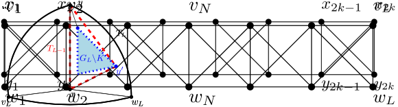
Figure 19: A graph with $k$ crossings that requires height at least $2k$ in any planar drawing.

Note that the graph used in the example above has pathwidth $3$; thus this crossing number lower bound is not subsumed by the pathwidth lower bound.

0.E.3 More constructions

We now give the details that lead to Theorem 6.4. As in Section 4 we assume that our input graph $G$ is plane-maximal with a reference-edge $(s,t)$, and we choose some root-to-leaf path $\pi$ in ${\overline{G^{*}}}$. Let $P_{\pi}$ be the outer-1-path whose inner dual is $\pi$ and let $f_{st}$ be the face of ${\overline{P_{\pi}}}$ incident to $(s,t)$. At most one of $s$ and $t$ can belong to the face $f^{\prime}$ after $f_{st}$ on ${\overline{P_{\pi}}}$; up to symmetry we assume that $s$ does not belong to $f^{\prime}$. The enhanced $\pi$-path $P_{\pi}^{+}$ is the plane-maximal outer-1-path formed by $P_{\pi}$ together with all neighbours of $s$. Let $\hat{e}\neq(s,t)$ be an arbitrary outer-face edge on the leaf-face of $\pi$, and enumerate the outer face of $P_{\pi}^{+}$ as $x_{0},\dots,x_{\ell},y_{r},\dots,y_{0}$ where $\hat{e}=(x_{\ell},x_{r})$ and $(s,t)=(y_{0},y_{1})$. Note that (in contrast to Section 4) the end-edge is not $(s,t)$; instead it is the other outer-face edge incident to $s$.

Figure 20: Example-graph for constructing bar visibility representations. $P_{\pi}$ is shaded.

0.E.3.1 Drawing $P_{\pi}^{+}$.

We already discussed in Lemma 4 how to create a visibility representation of an outer-1-path, but now the situation is different because we want bars, rather than boxes. The canonical drawing of ${\overline{P_{\pi}^{+}}}$ is defined as follows (we adopt ideas from [5], but use an extra row). All bars for $x_{0},\dots,x_{\ell}$ are in row $-1$; all bars for $y_{1},\dots,y_{r}$ are in row $1$. We assign $x$-coordinates to the endpoints of these bars by parsing the faces $f_{1},\dots,f_{k}$ of ${\overline{P_{\pi}^{+}}}$ in order, beginning with the one incident to $(x_{0},y_{0})$. We use $b(u)$ for the bar representing $u$. Both $b(x_{0})$ and $b(y_{0})$ begin at $x$-coordinate 1. If face $f_{h}$ (for $h\geq 1$) contains no crossing, say $f_{h}=\{x_{i},x_{i+1},y_{j}\}$, then $b(x_{i})$ ends, $b(x_{i+1})$ begins and $b(y_{j})$ extends further rightwards. See e.g. $\{x_{2},x_{3},y_{2}\}$ in Fig. 21. If $f_{h}$ contains an opposite-boundary crossing, say $f_{h}=\{x_{i},x_{i+1},y_{j},y_{j+1}\}$, then $b(x_{i})$ ends and $b(x_{i+1})$ begins, and one unit further right $b(y_{j})$ ends end $b(y_{j+1})$ begins, see e.g. $\{x_{4},x_{5},y_{3},y_{4}\}$ in Fig. 21. Finally if $f_{h}$ contains a same-boundary crossing, say $f_{h}=\{x_{i},y_{j},y_{j+1},y_{j+2}\}$, then $b(y_{j})$ ends, $b(y_{j+1})$ begins and ends immediately again, and then $b(y_{j+2})$ begins, see e.g. $\{x_{6},y_{5},y_{6},y_{7}\}$ in Fig. 21.

Figure 21: Drawing the planar skeleton.

Observe that row 0, which we call the center row, remains empty, i.e., intersects no vertex. (We can delete empty rows in the final drawing, but maintaining it during the construction gives us a place to add further rows as needed.)

The resulting drawing $\Gamma_{P}$ represents ${\overline{P_{\pi}^{+}}}$, and, in order to draw $P_{\pi}^{+}$, we shall draw each pair of crossing edges. The method to do this depends on whether we have same-boundary crossings or opposite-boundary crossings and on the drawing model, and will be detailed in the following sections.

0.E.3.2 Inward merging.

As in Section 4, the idea is to merge hanging subgraphs of the path, but this time we merge “inward”. Assume that for each hanging subgraph we can recursively obtain a $TC_{1,1}$-drawing $\Gamma_{H}$, i.e., bars $b(u)$ and $b(v)$ occupy the top corners. Expand the center row into as many rows as needed for the hanging subgraphs. Then for each hanging subgraph $H$, we insert $\Gamma_{H}$ (possibly after rotation) in these new rows in such a way that the two drawings of the reference-edge of $H$ coincide. See Fig. 22. We remark that, when performing an inward merging, the outer-1-planar embedding is not respected (some vertices will not be on outer-face anymore). Inward merging was used in [5] to create drawings of outer-planar graphs with height $O(pw(G))$.

Figure 22: Inward merging. We shade the faces of ${\overline{P_{\pi}^{+}}}$ for easier identification later on.

0.E.3.3 Handling most same-boundary crossings.

Let $\Gamma_{P}$ be the canonical drawing of ${\overline{P_{\pi}^{+}}}$; here vertices $s,t$ are drawn at the left end of row 1 since $(s,t)=(y_{0},y_{1})$. We now show how to handle all same-boundary crossings except the one that may occur at face $f_{st}$. Add a new row each above and below the center-row. For a same-boundary crossing, let the middle vertex be the middle of the three vertices that are on the same boundary. For each same-boundary crossing (say at face $f\neq f_{st}$), move the middle vertex into the adjacent new row and re-route the incident edges of $f$ vertically after extending vertex bars as needed. The two crossing edges can now both be inserted; one horizontally in row 1 or $-1$, and the other one vertically. See Fig. 23.

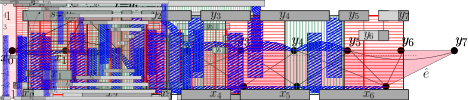
Figure 23: Handling most same-boundary crossings. Edges in crossings are red (bold). Light gray boxes are extensions of existing vertex-boxes.

We must be careful to keep space available for merging hanging subgraphs later. We say that an edge $(u,v)$ permits merging in one of the following two cases. Either $(u,v)$ is drawn horizontally, and the axis-aligned rectangle between $(u,v)$ and the center-row is empty. Alternatively, $(u,v)$ is drawn vertically, both its ends are on the same side of the center-row, and if (say) $v$ is closer to the center-row than $u$, then $b(v)$ ends at $(u,v)$, and there is an axis-aligned empty rectangle where one horizontal side is $u$, the other horizontal side is on the center, and one vertical side contains $(u,v)$. In the canonical drawing all edges that might have hanging subgraphs were drawn horizontally and permitted merging. One verifies that edges that are now drawn vertically (due to a same-boundary crossing) likewise permit merging.

0.E.3.4 Handling the remaining crossings.

Now consider an opposite-boundary crossing, say at face $\{x_{i},$ $x_{i+1},$ $y_{j},$ $y_{j+1}\}$. None of $\{x_{i},$ $x_{i+1},$ $y_{j},$ $y_{j+1}\}$ is the middle vertex of a same-boundary crossing, so these vertices are in rows 2 and $-2$, respectively. Handling opposite-boundary crossings, as well as the same-boundary crossing at $f_{st}$, is the only part where the drawing-algorithm depends on the drawing-model.

Planar bar visibility representations.

For planar bar visibility representations, we handle opposite-boundary crossings by moving vertices outward to new rows, and inserting one of each pair of crossings at the extreme right end of the drawing. Specifically, at any opposite-boundary crossing at a face $\{x_{h},x_{h+1},y_{z},y_{z+1}\}$, mark $x_{h}$ and $y_{z+1}$. Also, if $f_{st}$ is a same-boundary crossing, then it is of the form $f_{st}=\{s,t,y_{1},x_{\rho}\}$ for some index $\rho$ and we mark $y_{1}$ and $x_{\rho}$. Finally, mark $t$ if it was not marked yet.

See Fig. 24 for the following process. For any vertex $v$, let $m(v)$ be the total number of marks at $v$ or at vertices further right on the same boundary as $v$. We move $y_{z}$ upwards by $m(y_{z})$ rows and we move $x_{h}$ downwards by $m(x_{h})$ rows (inserting new rows as needed and re-routing outer-face edges so that they permit merging). If $\chi_{P}$ is the number of crossings in $P_{\pi}^{+}$, then the total number of rows is now at most $4+2\chi_{P}$: We started with 3 rows originally, added one row because we marked $t$, add two rows total for same-boundary crossings (but need those only if there are actually such crossings), and then two more rows for each remaining crossings.

We restore edges and insert the missing crossings in order from right to left, i.e., by decreasing index on the boundary. Consider an opposite-boundary-crossing at face $f=\{x_{h},x_{h+1},y_{z},y_{z+1}\}$. Vertices $x_{h}$ and $y_{z+1}$ was marked, hence $b(y_{z+1})$ is higher than the bars of $y_{z+2},\dots,y_{r}$ while $b(x_{h})$ is lower than the bars of $x_{h+1},\dots,x_{\ell}$. We can hence expand both $y_{z+1}$ and $x_{h}$ rightward beyond everything drawn in the rows between them and insert $(x_{h},y_{z+1})$ as a vertical edge at the very right end of the drawing. We can also draw $(x_{h+1},y_{z})$ vertically within $f$, after expanding $x_{h}$ and $y_{z+1}$ towards each other if needed.

Figure 24: Handling the remaining crossings by adding rows for a planar bar visibility representation. Dotted arrows indicate vertices that are marked.

If $f_{st}$ is a same-boundary crossing, then $t$ and $x_{\rho}$ were both marked, and so can be expanded rightward and $(t,x_{\rho})$ can be drawn vertically at the very right end of the drawing. Also, edge $(s,y_{2})$ is drawn vertically within $f_{st}$, by expanding $s$ and $y_{2}$ towards each other. We also marked $y_{2}$, and did this so that $b(y_{2})$ likewise can be expanded to the right; then outer-face edge $(y_{2},t)$ can be drawn at the right end to permit merging.

Note that $t$ is always marked and that $s$ is never marked, so $m(t)=m(s)$ and $s,t$ are both in the topmost row and no other vertex is in that row. If needed, we can expand $t$ to cover the rightmost endpoint. We hence have:

Lemma 8.

For any root-to-leaf path $\pi$ in ${\overline{G^{*}}}$, graph $P_{\pi}^{+}$ has a planar bar visibility representations on at most $4+2\chi(P_{\pi}^{+})$ rows that is a $C_{1,1}$-drawing.

Furthermore, the center row is empty, and any edge that could have an attached hanging subgraph permits merging.

Bar-1-visibility representations.

For bar-1-visibility representations, we change the drawing as illustrated in Fig. 25. First we add three new rows above and one new row below, so that we now have rows $-3,\dots,5$. Parse the bars in row $-2$ left to right (these are the bars $b(x_{0}),\dots,b(x_{\ell})$, except those of middle vertices of opposite-boundary crossings). Move every second of these bars into row $-3$. We can choose to move $b(x_{0})$ or not, and do this choice as follows. If $f_{st}$ contains an opposite-boundary crossing, say $f_{st}=\{x_{\rho},x_{\rho+1},s,t\}$ then we do the choice such that $x_{\rho}$ ends in row $-3$; otherwise the choice is arbitrary. Any outer-face edge $(x_{h},x_{h+1})$ can be re-routed vertically (after extending bars of its endpoints towards each other) and then still permits merging.

As for the bars in row 2, we move both $b(s)$ and $b(t)$ into row $5$. We move $b(y_{2})$ (if it is in row 2) into row $4$, and move every other of the remaining bars of row 2 into row 3. This makes all edges (except $(s,t)$) vertical, as required for a bar-1-visibility representation.

We first handle the same-boundary crossing at $f_{st}$ (if it exists). Assume that this is $f_{st}=\{s,t,y_{2},x_{\rho}\}$. Since $b(t)$ is on row 5 and $b(y_{2})$ is on row 4, we can route $(t,x_{\rho})$ by traversing $b(y_{2})$, while $(s,y_{2})$ can be routed inside $f_{st}$ after extending the vertices towards each other. As for planar bar visibility representations, we also expand both $b(t)$ and $b(y_{2})$ rightwards and route outer-face edge $(t,y_{2})$ at the right end so that it permits merging. See Fig. 25.

Now parse the opposite-boundary crossings from left to right. Say we handle crossing edges $(x_{h},y_{z+1})$ and $(y_{z},x_{h+1})$. If $b(x_{h})$ is in row $-3$, then we expand $b(x_{h})$ rightwards beyond edge $(x_{h},x_{h+1})$ and draw $(x_{h},y_{z+1})$ by traversing $b(x_{h+1})$ (which is in a higher row since we alternate). See e.g. $\{x_{4},x_{5},y_{3},y_{4}\}$ in Fig. 25. Note that this case always applies if $f_{st}$ contains a opposite-boundary crossing because $b(x_{\rho})$ is placed in row $-3$.

If $b(x_{h})$ is in row $-2$, but $b(y_{z})$ is higher than $b(y_{z+1})$, then similarly we can expand $b(y_{z})$ rightwards beyond $(y_{z},y_{z+1})$ and draw $(y_{z},x_{h+1})$ by traversing $b(y_{z+1})$. See e.g. $\{x_{3},x_{4},y_{2},y_{3}\}$ in Fig. 25.

The only case that is more difficult is when $b(x_{h})$ is on row $-2$ and $y_{z}$ is on row $2$. See e.g. $\{x_{5},x_{6},y_{4},y_{5}\}$ in Fig. 25. Bars $b(x_{h})$ and/or $b(y_{z})$ may already have been traversed when handling an opposite-boundary crossing further left, so we must be careful not to traverse it again. However, $b(x_{h})$ is traversed by an edge only if the last handled opposite-boundary crossing was at face $\{x_{h-1},x_{h},y_{\ell},y_{\ell+1}\}$ for some $\ell<j$. In this case, none of $b(y_{\ell+1}),\dots,b(y_{z})$ are traversed, because $b(y_{\ell+1})$ is not traversed at the crossing if $b(x_{h})$ is, and there are no other opposite-boundary crossings involving $y_{\ell+1},\dots,y_{z}$. So at least one of $b(x_{h}),b(y_{z})$ has not been traversed. Route one of the crossing edges to traverse that bar (after extending either $b(x_{h+1})$ or $b(y_{z+1})$ leftward).

So in all cases we can draw one of the two crossing edges $(x_{h},y_{z+1})$ and $(y_{z},x_{h+1})$ by traversing one bar of the four vertices. The other edge of the crossing can be inserted within the face vertically, by extending its endpoints towards each other.

Figure 25: Handling the remaining crossings for bar-1-visibility representations.

Note that by construction $s$ and $t$ are the only vertices in the topmost row, and we can expand $b(t)$ to cover the rightmost corner. We hence have:

Lemma 9.

For any root-to-leaf path $\pi$ in ${\overline{G^{*}}}$, $P_{\pi}^{+}\setminus(s,t)$ has a bar-1-visibility representation on 8 rows that is a $C_{1,1}$-drawing.

Furthermore, the center row is empty, and any edge that could have an attached hanging subgraph permits merging.

0.E.3.5 Putting it all together.

We now put these path-drawings together with drawings of the hanging subgraphs by merging inward.

Theorem 6.4.

Every outer-1-plane graph $G$ has a planar bar visibility representation of area $O((pw(G){+}\chi(G))n)$ and a bar-1-visibility representation of area $O(n{\cdot}pw(G))$.

Proof.

We first need a small detour to explain how to choose path $\pi$. Pick an arbitrary reference-edge $(s,t)$, and let $T$ be the inner tree ${\overline{G^{*}}}$, rooted at $f_{st}$. We define the rooted pathwidth $rpw(T)$ to be 1 if $T$ has exactly one leaf, and $rpw(T)=\min_{\pi}\max_{T^{\prime}\in\mathcal{T}(T,\pi)}\{1+rpw(T^{\prime})\}$ otherwise, where the minimum is over all root-to-leaf paths $\pi$, and $\mathcal{T}(T,\pi)$ is the set of rooted subtrees obtained by deleting the vertices of $\pi$ from $T$. The path $\pi$ that achieves the minimum is called a spine and satisfies that $rpw(T^{\prime})<rpw(T)$ for all $T^{\prime}\in\mathcal{T}(T,\pi)$. See [8] for details.

We now prove (by induction on $rpw(T)$) that we have

• a planar bar visibility representation with height at most $2rpw(T)+2\chi+1$,

• a bar-1-visibility representation of $G\setminus(s,t)$ with height at most $6rpw(T)+1$.

Furthermore, these are $C_{1,1}$-drawings. In the base case, $rpw(T)=1$, so $G$ is an outer-1-path and the result holds by Lemma 8 and 9 since we can delete the empty center-row. So assume $rpw(T)>1$, and let $\pi$ be a spine of $T$. Apply Lemma 8 and 9, respectively, to obtain drawing $\Gamma_{P}$ of $P_{\pi}^{+}$. Apply induction to any hanging subgraph $H$ to obtain its drawing $\Gamma_{H}$.

In $\Gamma_{H}$, bars $b(u),b(v)$ of the reference-edge $(u,v)$ occupy the top corners. In $\Gamma_{P}$, $(u,v)$ permits merging. If $(u,v)$ is drawn horizontally in $\Gamma_{P}$, then we can simply merge the drawing inward, after adding sufficiently many new rows at the center-row. If $(u,v)$ is drawn vertically in $\Gamma_{P}$, say with (up to symmetry) both $u,v$ above the center-row and $u$ above $v$ by $Y\geq 0$ rows, then simply raise $u$ in $\Gamma_{H}$ by $Y$ rows and call the result $\Gamma_{H}^{\prime}$. Then the placement of $u$ and $v$ is the same in $\Gamma_{P}$ and $\Gamma_{H}^{\prime}$ (up to rotation) and so again after adding new rows as needed at the center row $\Gamma_{H}^{\prime}$ can be merged.

The number of new rows that we need for the subgraphs is no more than $\max_{H}\{\mathit{height}(\Gamma_{H})-2\}$: we already had the (empty) center-row that we can use, and we do not need space row of $b(u)$ and $b(v)$ (or all other rows added for $\Gamma_{H}^{\prime}$) since these reuse rows that already exist in $\Gamma_{P}$.

For bar-1-visibility representations, $\Gamma_{P}$ used 8 rows and each $\Gamma_{H}$ has height at most $6(rpw(T)-1)+1$ by induction since the rooted pathwidth of ${\overline{H^{*}}}$ is smaller. So the height is at most $8+(6rpw(T)-5)-2=6rpw(T)+1$ as desired. For bar visibility representations, $\Gamma_{P}$ used $4+2\chi_{P}$ rows, and each hanging subgraph has at most $\chi-\chi_{P}$ crossings and hence height at most $2(rpw(T)-1)+2(\chi-\chi_{P})+1$. So the total height is at most $2rpw(T)+2\chi+1$ as desired.

By induction our claim holds. It is well-known that $rpw(T)\leq 2pw(T)+1$ [8] and that $pw(T)\leq pw(G)$ [15]. So we create drawings of height proportional to $pw(G)$ and $pw(G)+\chi$, respectively. For bar-1-visibility representations, currently edge $(s,t)$ is missing, but it can be inserted horizontally, and then be made vertical by moving one of $s$ and $t$ up into a new row. This proves the theorem since the width is $O(n)$ by Obs. 1. ∎

References

- [1] Angelini, P., Bekos, M.A., Kaufmann, M., Montecchiani, F.: On 3D visibility representations of graphs with few crossings per edge. Theor. Comput. Sci. 784, 11–20 (2019)
- [2] Arleo, A., Binucci, C., Di Giacomo, E., Evans, W.S., Grilli, L., Liotta, G., Meijer, H., Montecchiani, F., Whitesides, S., Wismath, S.K.: Visibility representations of boxes in 2.5 dimensions. Comput. Geom. 72, 19–33 (2018)
- [3] Auer, C., Bachmaier, C., Brandenburg, F., Gleißner, A., Hanauer, K., Neuwirth, D., Reislhuber, J.: Outer 1-planar graphs. Algorithmica 74(4), 1293–1320 (2016)
- [4] Biedl, T.: Small drawings of outerplanar graphs, series-parallel graphs, and other planar graphs. Discrete Comput. Geom. 45(1), 141–160 (2011)
- [5] Biedl, T.: A 4-approximation algorithm for the height of drawing 2-connected outerplanar graphs. In: Erlebach, T., Persiano, G. (eds.) WAOA. LNCS, vol. 7846, pp. 272–285. Springer (2013)
- [6] Biedl, T.: Height-preserving transformations of planar graph drawings. In: Duncan, C., Symvonis, A. (eds.) GD. LNCS, vol. 8871, pp. 380–391. Springer (2014)
- [7] Biedl, T.: Drawing outer-1-planar graphs revisited. In: Auber, D., Valtr, P. (eds.) GD. LNCS, vol. 12590, pp. 526–527. Springer (2020), Poster. Full-length version available at CoRR 2009.07106
- [8] Biedl, T.: Horton-Strahler number, rooted pathwidth and upward drawings of tree (2021), accepted pending revisions at Information Processing Letters. Preliminary version appeared at CoRR 1506.02096
- [9] Biedl, T., Chaplick, S., Kaufmann, M., Montecchiani, F., Nöllenburg, M., Raftopoulou, C.: On layered fan-planar graph drawings. In: Esparza, J., Král’, D. (eds.) MFCS 2020. LIPIcs, vol. 170, pp. 14:1–14:13. LZI (2020)
- [10] Biedl, T., Demontigny, P.: A 2-approximation for the height of maximal outerplanar graphs. In: Ellen, F., Kolokolova, A., Sack, J. (eds.) WADS. Lecture notes in computer science, vol. 10389, pp. 145–156. Springer (2017)
- [11] Biedl, T., Kaufmann, M.: Area-efficient static and incremental graph drawings. In: Burkard, R.E., Woeginger, G.J. (eds.) ESA. LNCS, vol. 1284, pp. 37–52. Springer (1997)
- [12] Biedl, T., Montecchiani, F., Liotta, G.: Embedding-preserving rectangle visibility representations of nonplanar graphs. Discrete Comput. Geom. 60(2), 345–380 (2018)
- [13] Biedl, T., Liotta, G., Lynch, J., Montecchiani, F.: Generalized LR-drawings of trees. In: Canadian Conference on Computational Geometry (CCCG). pp. 78–88 (2021)
- [14] Bläsius, T., Brückner, G., Rutter, I.: Complexity of higher-degree orthogonal graph embedding in the Kandinsky model. In: Schulz, A.S., Wagner, D. (eds.) ESA. LNCS, vol. 8737, pp. 161–172. Springer (2014)
- [15] Bodlaender, H.L., Fomin, F.: Approximation of pathwidth of outerplanar graphs. J. Algorithms 43(2), 190 – 200 (2002)
- [16] Bose, P., Everett, H., Fekete, S., Houle, M., Lubiw, A., Meijer, H., Romanik, K., Rote, G., Shermer, T., Whitesides, S., Zelle, C.: A visibility representation for graphs in three dimensions. J. Graph Algorithms Appl. 2(3), 1–16 (1998)
- [17] Brandenburg, F.J.: 1-visibility representations of 1-planar graphs. J. Graph Algorithms Appl. 18(3), 421–438 (2014)
- [18] Brandenburg, F.J.: T-shape visibility representations of 1-planar graphs. Comput. Geom. 69, 16–30 (2018)
- [19] Brandenburg, F.J., Heinsohn, N., Kaufmann, M., Neuwirth, D.: On bar (1, j)-visibility graphs. In: Rahman, M.S., Tomita, E. (eds.) WALCOM. LNCS, vol. 8973, pp. 246–257. Springer (2015)
- [20] Chan, T.M.: A near-linear area bound for drawing binary trees. Algorithmica 34(1), 1–13 (2002)
- [21] Dean, A.M., Evans, W.S., Gethner, E., Laison, J.D., Safari, M.A., Trotter, W.T.: Bar -visibility graphs. J. Graph Algorithms Appl. 11(1), 45–59 (2007)
- [22] Dehkordi, H.R., Eades, P.: Every outer-1-plane graph has a right angle crossing drawing. Int. J. Comput. Geom. Appl. 22(6), 543–558 (2012)
- [23] Di Battista, G., Eades, P., Tamassia, R., Tollis, I.G.: Graph Drawing: Algorithms for the Visualization of Graphs. Prentice-Hall (1999)
- [24] Di Giacomo, E., Didimo, W., Evans, W.S., Liotta, G., Meijer, H., Montecchiani, F., Wismath, S.K.: Ortho-polygon visibility representations of embedded graphs. Algorithmica 80(8), 2345–2383 (2018)
- [25] Didimo, W., Liotta, G., Montecchiani, F.: A survey on graph drawing beyond planarity. ACM Comput. Surv. 52(1), 4:1–4:37 (2019)
- [26] Duchet, P., Hamidoune, Y.O., Vergnas, M.L., Meyniel, H.: Representing a planar graph by vertical lines joining different levels. Discret. Math. 46(3), 319–321 (1983)
- [27] Eggleton, R.: Rectilinear drawings of graphs. Util. Math. 29, 149–172 (1986)
- [28] Evans, W.S., Kaufmann, M., Lenhart, W., Mchedlidze, T., Wismath, S.K.: Bar 1-visibility graphs vs. other nearly planar graphs. J. Graph Algorithms Appl. 18(5), 721–739 (2014)
- [29] Evans, W.S., Liotta, G., Montecchiani, F.: Simultaneous visibility representations of plane -graphs using L-shapes. Theor. Comput. Sci. 645, 100–111 (2016)
- [30] Fan, J.H., Lin, C.C., Lu, H.I., Yen, H.C.: Width-optimal visibility representations of plane graphs. In: Tokuyama, T. (ed.) ISAAC. pp. 160–171. LNCS, Springer (2007)
- [31] Felsner, S., Liotta, G., Wismath, S.: Straight-line drawings on restricted integer grids in two and three dimensions. J. Graph Algorithms Appl. 7(4), 335–362 (2003)
- [32] Fößmeier, U., Kant, G., Kaufmann, M.: 2-visibility drawings of planar graphs. In: North, S. (ed.) GD. LNCS, vol. 1190, pp. 155–168. Springer (1997)
- [33] Frati, F., Patrignani, M., Roselli, V.: LR-drawings of ordered rooted binary trees and near-linear area drawings of outerplanar graphs. J. Comput. Syst. Sci. 107, 28–53 (2020)
- [34] He, X., Zhang, H.: Nearly optimal visibility representations of plane graphs. SIAM J. Discrete Math. 22(4), 1364–1380 (2008)
- [35] Hong, S., Eades, P., Katoh, N., Liotta, G., Schweitzer, P., Suzuki, Y.: A linear-time algorithm for testing outer-1-planarity. Algorithmica 72(4), 1033–1054 (2015)
- [36] Hong, S., Tokuyama, T. (eds.): Beyond Planar Graphs, Communications of NII Shonan Meetings. Springer (2020)
- [37] Kobourov, S., Liotta, G., Montecchiani, F.: An annotated bibliography on 1-planarity. Comput. Sci. Rev. 25, 49–67 (2017)
- [38] Liotta, G., Montecchiani, F.: L-visibility drawings of IC-planar graphs. Inf. Process. Lett. 116(3), 217–222 (2016)
- [39] Liotta, G., Montecchiani, F., Tappini, A.: Ortho-polygon visibility representations of 3-connected 1-plane graphs. Theor. Comput. Sci. 863, 40–52 (2021)
- [40] Otten, R., van Wijk, J.: Graph representations in interactive layout design. In: IEEE ISCS. pp. 914–918 (1978)
- [41] Rosenstiehl, P., Tarjan, R.E.: Rectilinear planar layouts and bipolar orientation of planar graphs. Discrete Comput. Geom. 1, 343–353 (1986)
- [42] Shermer, T.: Block visibility representations III: External visibility and complexity. In: CCCG. International Informatics Series, vol. 5, pp. 234–239. Carleton University Press (1996)
- [43] Tamassia, R., Tollis, I.: A unified approach to visibility representations of planar graphs. Discrete Comput. Geom. 1, 321–341 (1986)
- [44] Wismath, S.: Characterizing bar line-of-sight graphs. In: Snoeyink, J. (ed.) SoCG. pp. 147–152. ACM (1985)