A Comparison of Deep Saliency Map Generators on Multispectral Data in Object Detection

Abstract

Deep neural networks, especially convolutional deep neural networks, are state-of-the-art methods to classify, segment or even generate images, movies, or sounds. However, these methods lack of a good semantic understanding of what happens internally. The question, why a COVID-19 detector has classified a stack of lung-ct images as positive, is sometimes more interesting than the overall specificity and sensitivity. Especially when human domain expert knowledge disagrees with the given output. This way, human domain experts could also be advised to reconsider their choice, regarding the information pointed out by the system. In addition, the deep learning model can be controlled, and a present dataset bias can be found.

Currently, most explainable AI methods in the computer vision domain are purely used on image classification, where the images are ordinary images in the visible spectrum. As a result, there is no comparison on how the methods behave with multimodal image data, as well as most methods have not been investigated on how they behave when used for object detection.

This work tries to close the gaps. Firstly, investigating three saliency map generator methods on how their maps differ across the different spectra. This is achieved via accurate and systematic training. Secondly, we examine how they behave when used for object detection.

As a practical problem, we chose object detection in the infrared and visual spectrum for autonomous driving. The dataset used in this work is the Multispectral Object Detection Dataset [1], where each scene is available in the long-wave (FIR), mid-wave (MIR) and short-wave (NIR) infrared as well as the visual (RGB) spectrum.

The results show that there are differences between the infrared and visual activation maps. Further, an advanced training with both, the infrared and visual data not only improves the network’s output, it also leads to more focused spots in the saliency maps.

Keywords Object Detection  $\cdot$ Saliency Map Generators  $\cdot$ Multispectral Data

1 Introduction

Computer vision is no longer imaginable without convolutional deep neural networks. These methods provide excellent performance in image classification, segmentation and object detection, and are best known in the non-academic area for their usage in autonomous driving, intelligent video surveillance and human medicine. The increasing integration into daily life led to a rising demand for explainability and interpretability of those black box models. In recent years, a vast number of different methods [2, 3, 4, 5, 6, 7, 8, 9, 10] have been developed, that enable deep learning-based image classifiers to provide a visual explanation of their classification result.

Two big subsets of these explanation methods are gradient- and perturbation-based methods. The three investigated methods in this paper are also gradient- and perturbation-based: Grad-CAM [7] is a method, that combines gradient information with the feature maps of the last convolution layer of a CNN, to generate a saliency map for a specific output class. RISE [5] is a Monte Carlo method, that perturbs the input image and queries the network with the masked versions of the image. The resulting saliency map is the combination of each mask weighted by the corresponding prediction probability of the targeted class. Like Grad-CAM, the third method SIDU [9] uses the feature maps of the last convolution layer. These feature maps serve as masks for the input data. Similar to RISE, SIDU uses the network’s output to calculate a similarity difference and uniqueness score for each masked input. The final saliency map is the weighted sum of the feature maps, where the weights are given by the corresponding similarity differences and the uniqueness scores.

The three methods are commonly used for the classification task. We investigate not only how these methods perform in the different spectra, but we also use them to generate saliency maps for the predicted bounding boxes (see Figure 1). To the best of our knowledge, this is also the first comparison of saliency map generators in object detection.

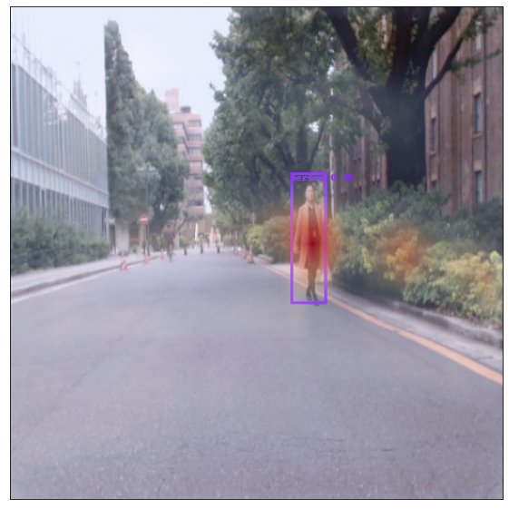
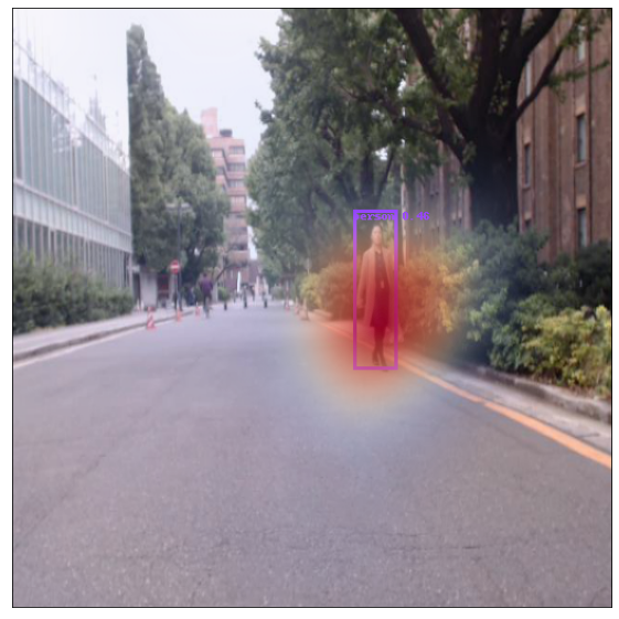
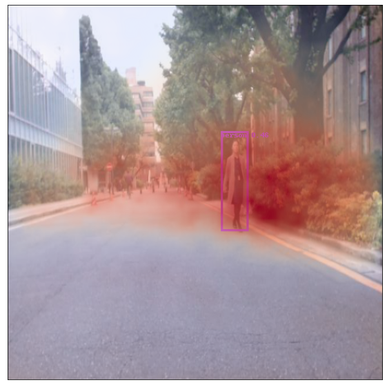
Figure 1: Saliency maps for the given bounding box, generated by Grad-CAM, RISE and SIDU.

2 Related Work

The following section covers selected work on object detection and explainable AI methods in the deep learning domain. For a comprehensive overview of shallow models, the reader is referred to a survey paper for object detection [11, 12] or explainable AI methods [13, 14, 15].

2.1 Object Detection

Deep learning-based object detection can generally be divided into one-stage and two-stage detectors [12, 16]. One-stage detectors predict bounding boxes directly from the given input image. Two-stage detectors have a preprocessing step to generate classification and regression proposals [17].

Faster R-CNN[18] is a two-stage object detector and introduced the Region Proposal Network (RPN). RPNs are fully convolutional networks, that predict bounding boxes as well as objectness scores. An RPN uses the attention [19] mechanism and is responsible for the higher throughput in comparison to the earlier Fast R-CNN [20] approach. The Single Shot MultiBox Detector (SSD) [21] is a one-stage object detector, that “discretizes the output space of bounding boxes into a set of default boxes over different aspect ratios and scales per feature map location”. YOLOv4 [22] is the fourth version of the famous one-stage detector framework. It combines a variety of “Bag-of-Freebies” and “Bag-of-Specials” like CIoU Loss [23] or Mish activation [24] to further improve speed and accuracy. With EfficientNet[25] as a backbone, and their proposed bi-directional feature pyramid network, EfficientDet [26] is a one-stage detector that is scalable and performant while maintaining high accuracy.

Recently, the research focus has shifted to the utilization of the underlying mechanisms of the transformer architecture [27, 28, 29].

2.2 Explainable AI

Most deep learning methods suffer from missing interpretability and explainability. Despite their potential good performance on test and validation data, the poor understanding of the internal processes leads to a lack of confidence in these methods. For the 2D image classification, there are methods to highlight areas in the image that are of special interest for the decision-making process of a convolutional neural network. These methods can generally be categorized into gradient-based, perturbation-based and other underlying mechanics.

Class Activation Maps (CAM)[30] are one of the earlier attempts to highlight the activations of the network. CAM requires a network to use global average pooling just before the fully connected layers. The final saliency map is then given by the weighted sum of the feature maps of the final convolution layer, where the weights are extracted from the fully connected layer for the target class.

Gradient-weighted Class Activation Mapping (Grad-CAM) [7] is a generalization of CAM and does not require a global average pooling. Instead, the method weights the upsampled feature maps of the ultimate convolution layer according to the gradient.

Sundararajan et al. [4] identify two axioms — Sensitivity and Implementation Invariance — that attribution methods should satisfy and present Integrated Gradients, a simple to implement method, that requires no modification to the original network and fulfills the named axioms. Integrated Gradients aggregates gradients along the straight line path between a reference image and the input image.

A combination of gradient- and perturbation-based method is SmoothGrad [2]. SmoothGrad samples Gaussian noised variations of the input image and averages the resulting gradient of these. In comparison to the vanilla gradient, the averaged gradient is much smoother and less noisy.

Randomized Input Sampling for Explanation (RISE) [31] is a perturbation-based method. The input image is masked with several random masks and propagated through the network. The final saliency map is then obtained as the weighted sum of the random masks, where the weights are given according to the output of the network for the corresponding perturbed input.

A similar yet different approach is SIDU [9]. During the forward propagation, the feature maps of the last convolution layer are extracted. The input is then masked with the extracted, upsampled feature maps and propagated through the network. For the resulting network outputs, a so-called similarity difference and uniqueness score[9] is calculated. The upsampled feature maps are then weighted according to the similarity difference and uniqueness scores and summed. The result is the saliency map for the predicted output.

Since DeconvNets [32] and Guided-Backpropagation [33] have been proven [34] to just do partial image reconstruction, they are not described further.

3 Saliency Map Generators

Saliency Map Generators visualize the activations of a convolutional neural network. Given an input image $\tensorsym{I}$ and a saliency map generator $f(\tensorsym{X})$, the saliency map $\matrixsym{S}=f(\tensorsym{I})$ highlights the most crucial areas for the decision process. In the following Section, we give a brief introduction about the examined saliency map generators: Grad-CAM [7], SIDU [9] and RISE [5].

3.1 Grad-CAM

Convolutional layers retain spatial information across consecutive layers. As a result, the ultimate convolution layer in a feed forward network contains the most dense spatial information of the image [7]. Based on the output feature maps of this layer, the input images are usually classified.

Grad-CAM uses the output features of this last convolution layer, to generate a saliency map. The method is a generalization of Class Activation Mapping (CAM) [30] and requires neither a fully convolutional network, nor a global average pooling layer [7]. Instead, a weighted sum of the extracted feature maps from the last convolution layer is calculated and bilinear upsampled.

Let $\tensorsym{F}\in\mathbb{R}^{N\times w\times h}$ be the output feature map of the ultimate convolution layer $l$. We then propagate the gradient $\tensorsym{G}^{c}$ for the target output class $c$ back to $l$. Finally, the saliency map

$$\matrixsym{S}^{c}=\sum_{i=1}^{N}ReLU(\alpha^{c}_{i}\cdot\matrixsym{F}_{i})$$ (1)

can be calculated, where the weights

$$\alpha^{c}_{i}=\frac{1}{w\cdot h}\sum_{u}^{w}\sum_{v}^{h}\tensorsym{G}^{c}_{u,v}$$ (2)

for each feature map $\matrixsym{F}_{i}$ are given as the mean of the corresponding gradients.

3.2 RISE

Instead of internal feature maps or gradient information, RISE perturbs the input and uses the output class probabilities of the network for the perturbed input as weights for the resulting saliency map. Compared to Grad-CAM, RISE has a significantly higher computational cost. The reason for this is that RISE requires a forward propagation for each perturbation mask $\matrixsym{M}_{i}$. First, $N$ small binary masks are sampled according to a distribution $\mathcal{D}$. The masks are then bilinear upsampled to be slightly larger, then the input size. Afterwards, the masks are randomly cropped to match the input size. For each generated mask $\matrixsym{M}_{i}$, the network output $\vectorsym{p}_{i}$ of the masked input image

$$\tensorsym{\tilde{I}}_{i}=\matrixsym{M}_{i}\circ\tensorsym{I}$$ (3)

is calculated. The saliency map

$$\matrixsym{S}^{c}=\frac{1}{\mathbb{E}[\tensorsym{M}]\cdot N}\sum_{i=1}^{N}\vectorsym{p}^{c}_{i}\cdot\matrixsym{M}_{i}$$ (4)

is then given as the sum of the upsampled masks, weighted by the corresponding probability score of the selected class and normalized by the expectation of M.

3.3 SIDU

In contrast to Grad-CAM and RISE, SIDU is incapable of generating a saliency map for a specific class. Instead, the generated saliency map highlights the image areas with the highest impact on the output feature vector. To achieve this, SIDU uses the feature maps $\matrixsym{F}_{i}$ of the last convolution layer to mask the input data. Those feature maps are bilinear upsampled to match the input size. Afterwards, the Hadamard product of the input $\tensorsym{I}$ and each mask $\matrixsym{M}_{i}$ is propagated through the network. The saliency map is the weighted sum of the masks, where the weights are calculated according to the masks impact on changes in the similarity difference

$$sd_{i}=exp(\frac{-1}{2\sigma^{2}}\cdot\lVert\vectorsym{p}_{o}-\vectorsym{p}_{i}\rVert)$$ (5)

and uniqueness scores

$$u_{i}=\sum_{j=1}^{N}\lVert\vectorsym{p}_{i}-\vectorsym{p}_{j}\rVert$$ (6)

of the network’s output $\vectorsym{p}$, regarding the unmasked input:

$$S^{c}=\sum_{i=1}^{N}sd_{i}\cdot u_{i}\cdot\matrixsym{M}_{i}$$ (7)

Here, $\vectorsym{p}_{o}$ is the network’s output for the unmasked input.

4 Experimental Setup

4.1 EfficientDet

For each spectrum, an EfficientDet-D0 is trained. The networks are trained via Adam [35] over thirty epochs, with an initial learning rate of 0.001 and a learning rate reduction by a factor of ten each tenth epoch. The used batch size is eight. The raw images of the dataset are split with a ratio of 1:4 in a test and train set and resized to a fixed size of $512\times 512$ pixel. The single channel of the infrared images is tripled to be compatible with the network’s input layer.

For the evaluation, the trained detectors are applied for each input image of the corresponding test set. For each image, the bounding box with the highest score is selected and investigated. Since SIDU and RISE sample the network multiple times with modified input data, the selected bounding box has to be found again. This is achieved via a search over all bounding boxes with a score of at least 0.05 and an intersection over union (IoU) of at least 0.5. The bounding box with the highest IoU is selected as the corresponding bounding box.

For the calculation of the saliency maps, the network’s output, especially the bounding box scores, are used. The feature maps that are required by Grad-CAM and SIDU are extracted directly from the classifier head. Since the ReLU activation in Equation 1 leads to empty or almost empty activation maps, Appendix A contains also the results without the ReLU activation. RISE uses 500 masks with a sample size of $8\times 8$ and a probability of $0.1$ for a pixel to be non-zero.

4.2 Dataset

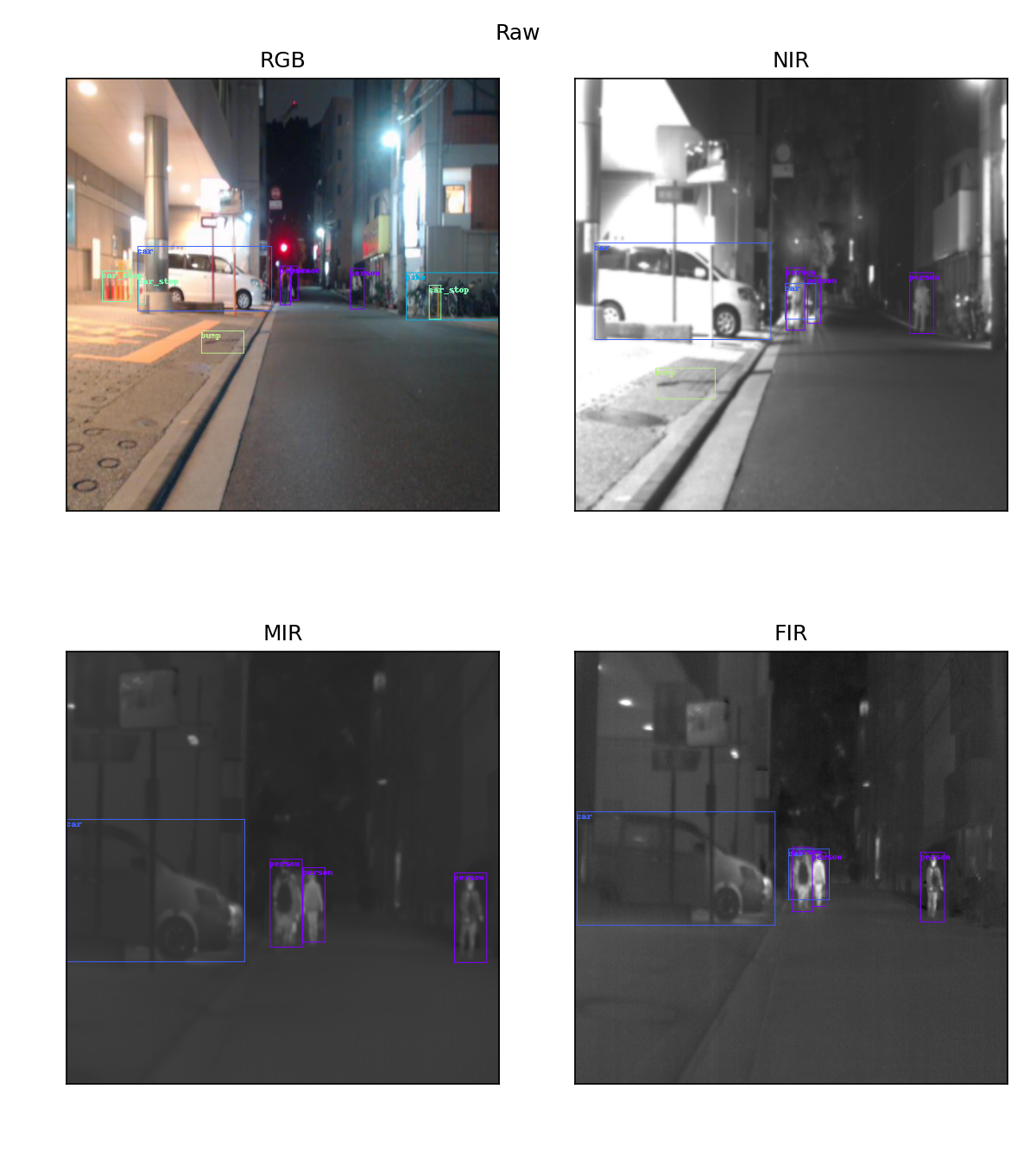
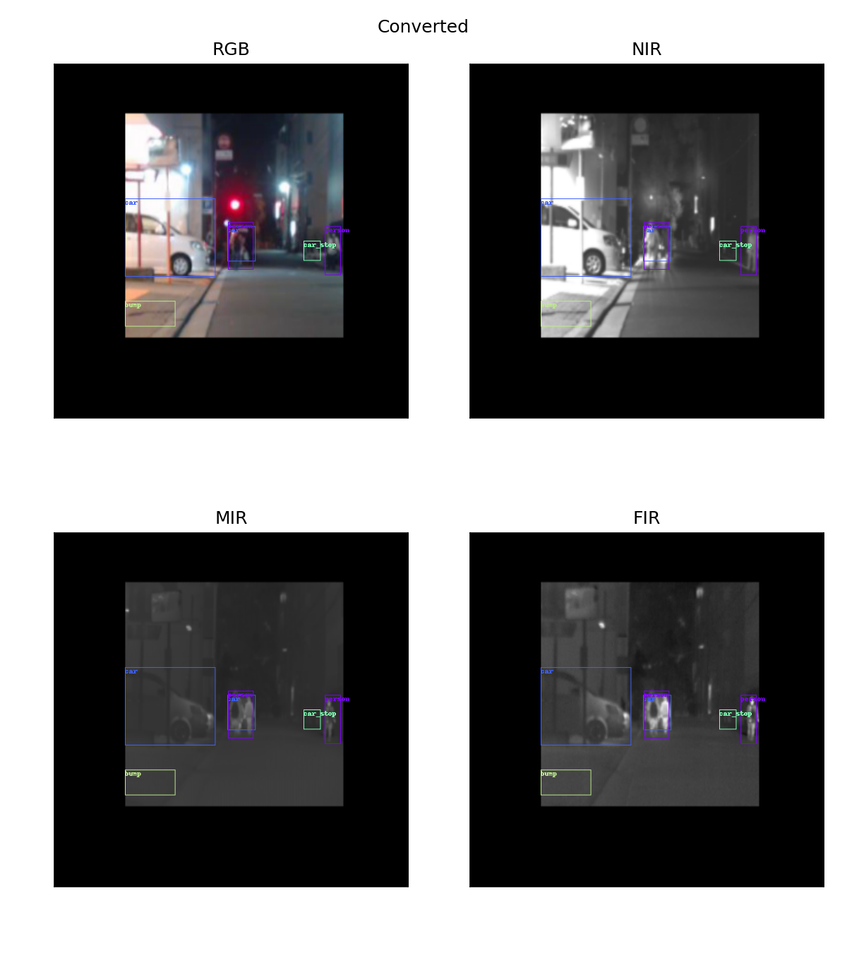
Figure 2: Examples of the Multispectral Dataset [1]. The same scene in different spectra: RGB, NIR, MIR and FIR. The raw images, which are used for the experiments, are given on the left half. Converted images with a common viewpoint are given on the right half.

To ensure an accurate and systematic training, we used the Multispectral Object Detection Dataset [1]. The dataset contains sequences, recorded in a university environment during day and nighttime. The sequences were captured with four cameras (RGB, NIR, MIR, FIR) and a frame rate of one frame per second. Since the viewpoints of the cameras are different, the dataset also contains converted versions of the images, where they share a common viewpoint (see Figure 2).

Table 1 contains the resolution of the images for the different spectra.

Spectrum	Width (px)	Height (px)
RGB	640	480
NIR	320	256
MIR	320	256
FIR	640	480

Table 1: Raw image sizes of the Multispectral Object Detection dataset.

The ground truth is given in form of bounding boxes with the corresponding classes: Person, car, bike, color_cone, car_stop, bump, hole, animal, unknown.

5 Evaluation

For a quantitative comparison of the methods, the insertion, and deletion metrics[5] are used. The deletion metric removes pixels of the input successively according to their importance for a given saliency map. As a result, the probability of the predicted class decreases, the more pixels are removed. If the threshold is plotted against the output probability, the area under the resulting curve gives information about the performance of the method. If the most crucial pixels for the decision are removed first, there is a sharp drop in the curve and the area under the curve is close to zero. For the insertion metric, clear pixels are successively added to a blurred version of the original input image. In the optimal case, the area under the curve of the resulting plot is close to one and has therefore an early sharp rise. Appendix A contains plots of the deletion and insertion metrics for the different methods and spectra.

As stated in Table 2, the lowest total deletion score is achieved with SIDU and NIR data ($0.10\pm 0.03$). The highest total insertion score is also achieved with SIDU, but with RGB+MIR data ($0.67\pm 0.21$). The results also show that Grad-CAM has a significant higher mean deletion score and standard deviation than the other two methods. This is similar to the lower mean insertion score of Grad-CAM. Both, SIDU and RISE achieve similar results for the deletion and insertion metric, whereas SIDU performs slightly better.

Figure 3 shows generated saliency maps for a bounding box in the same scene but different spectra. Qualitatively, the saliency maps of Grad-CAM are mostly a single sharp focus spot. The reason for this is the application of the ReLU in Equation 1. Figure 1 and the figures in Appendix A are examples of Grad-CAM saliency maps, without the ReLU activation. A larger, more diffuse single focus spot is given in the saliency maps, generated by RISE. Like Grad-CAM, the queried bounding box always contains the center of the focus spot. Saliency maps generated via Grad-CAM without ReLU have multiple smaller focus spots, where the main focus is almost always in the queried bounding box as well. SIDU, on the other hand, generates much diffuser saliency maps, that are significant larger.

Figure 4 shows the saliency maps for the same scene as in Figure 3, but this time generated by a single network trained with RGB and MIR data. For Grad-CAM, the saliency maps have become larger. Especially, the maps for RGB and NIR are now visible. The saliency maps generated by RISE have become smaller and adapt more to the shape of the object inside the bounding box. SIDU also profits from the extended training: The saliency maps are a bit smaller and contain more focused areas. Nonetheless, the saliency maps of SIDU still seem to focus random areas. The reason for this is, that SIDU in its original implementation is not using any additional information of the target like RISE or Grad-CAM. When using SIDU in a classification task, the resulting saliency map can not be generated for a specified class. Instead, the method “visual explanations for the prediction” [9].

When comparing RGB and infrared saliency maps, the focus areas of the RGB saliency maps are diffuser than the infrared ones.

In terms of computation speed, Grad-CAM (0.1 seconds) is much faster than SIDU (8.5 seconds) or RISE (32 seconds, 5000 masks, 24 mask batch) on our test system (Intel i9-9980XE, Nvidia Quadro RTX 6000). For a real-time application, Grad-CAM is therefore the only applicable approach.

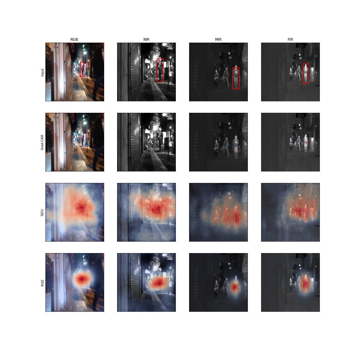
Figure 3: Generated saliency maps for raw images of different spectra. The top row shows the original images with the queried bounding box. The following rows show the saliency maps, generated by Grad-CAM, RISE and SIDU.

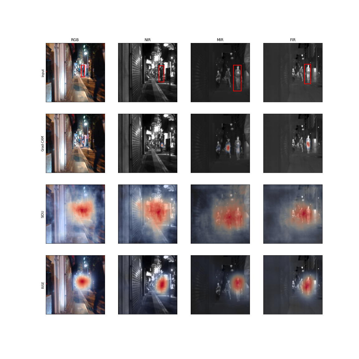
Figure 4: Generated saliency maps for raw images of different spectra with the trained RGB+MIR network. The top row shows the original images with the queried bounding box. The following rows show the saliency maps, generated by Grad-CAM, RISE and SIDU.

	Deletion $\downarrow$	Insertion $\uparrow$
Grad-CAM RGB	$0.22\pm 0.24$	$0.30\pm 0.14$
RISE RGB	$0.13\pm 0.05$	$0.34\pm 0.13$
SIDU RGB	$0.11\pm 0.04$	$0.38\pm 0.14$
Grad-CAM NIR	$0.23\pm 0.24$	$0.34\pm 0.14$
RISE NIR	$0.12\pm 0.05$	$0.34\pm 0.13$
SIDU NIR	$\mathbf{0.10\pm 0.03}$	$0.38\pm 0.13$
Grad-CAM MIR	$0.47\pm 0.26$	$0.47\pm 0.21$
RISE MIR	$0.15\pm 0.06$	$0.54\pm 0.20$
SIDU MIR	$0.13\pm 0.03$	$0.58\pm 0.18$
Grad-CAM FIR	$0.53\pm 0.29$	$0.52\pm 0.22$
RISE FIR	$0.17\pm 0.07$	$0.61\pm 0.20$
SIDU FIR	$0.15\pm 0.05$	$0.61\pm 0.20$
Grad-CAM RGB + MIR	$0.60\pm 0.31$	$0.53\pm 0.27$
RISE RGB + MIR	$0.25\pm 0.12$	$0.64\pm 0.22$
SIDU RGB + MIR	$0.20\pm 0.08$	$\mathbf{0.67\pm 0.21}$

Table 2: Mean and standard deviation of the deletion and insertion metrics for the different methods and models on evaluation data. The $\uparrow$/$\downarrow$ arrow indicates, whether a higher or lower score is desired.

6 Conclusion

This paper compares deep saliency map generators in object detection when used with multispectral data. As an object detector, EfficientDet has exemplarily been investigated. The experiments and evaluation show that the methods can easily be applied to the given task and result in similar but slightly distinguishable saliency maps for the different spectra. Grad-CAM and RISE show, most of the time, a single clear focus on the area around the questioned bounding box, while SIDU seems to also highlight unnecessary areas. When trained on both, RGB and MIR images, the main focus of the saliency methods is more focussed than on the separated training. Although the quantitative evaluation shows, that SIDU achieves the lowest deletion and highest insertion score, RISE offers the most obvious saliency map. In terms of usability in a real-time environment, only Grad-CAM can be calculated within a reasonable time. Further research could investigate how these methods perform on volumetric or spatio-temporal input data like CT scans or videos.

Appendix A Results

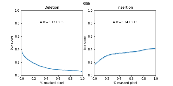
Figure 5: Insertion and Deletion evaluation of Grad-CAM, RISE and SIDU on RGB data.

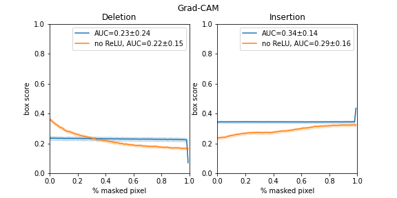
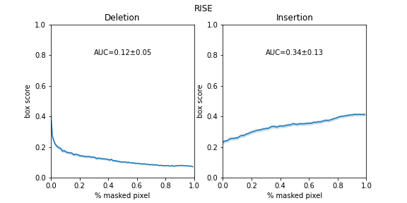
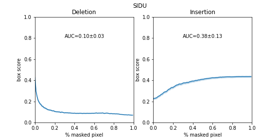
Figure 6: Insertion and Deletion evaluation of Grad-CAM, RISE and SIDU on NIR data.

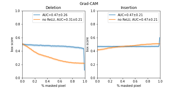
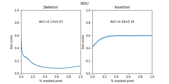
Figure 7: Insertion and Deletion evaluation of Grad-CAM, RISE and SIDU on MIR data.

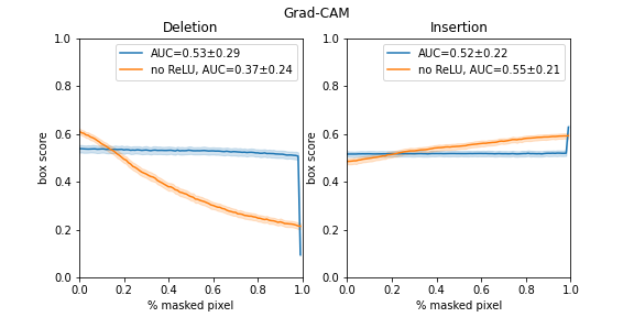
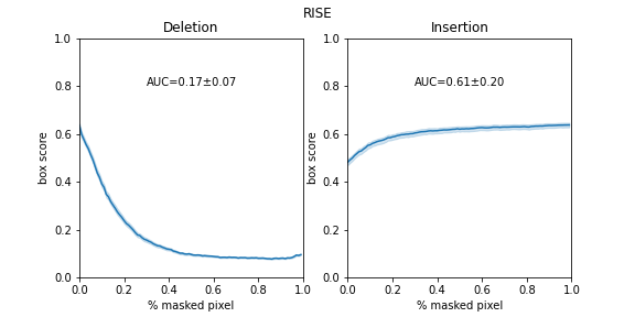
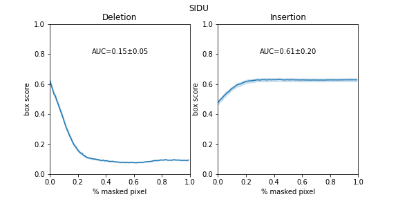
Figure 8: Insertion and Deletion evaluation of Grad-CAM, RISE and SIDU on FIR data.

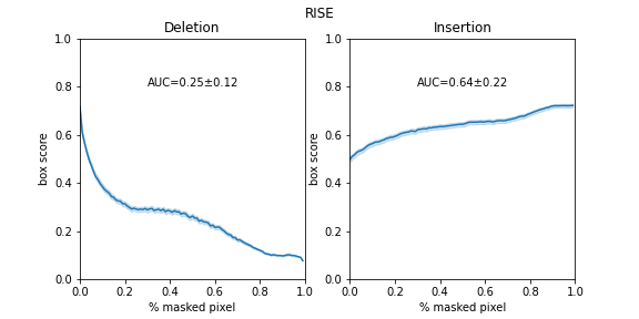
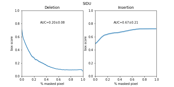
Figure 9: Insertion and Deletion evaluation of Grad-CAM, RISE and SIDU on RGB + MIR data.

Figure 10: Generated saliency maps for raw images of different spectra. The top row shows the original images with the queried bounding box. The second row shows the saliency maps, generated by Grad-CAM without the ReLU activation.

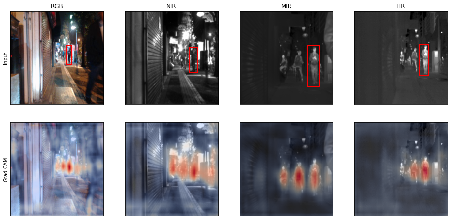
Figure 11: Generated saliency maps for raw images of different spectra with the trained RGB+MIR network. The top row shows the original images with the queried bounding box. The second row shows the saliency maps, generated by Grad-CAM without the ReLU activation.

References

- [1] Karasawa Takumi, Kohei Watanabe, Qishen Ha, Antonio Tejero-De-Pablos, Yoshitaka Ushiku, and Tatsuya Harada. Multispectral Object Detection for Autonomous Vehicles. In Proceedings of the on Thematic Workshops of ACM Multimedia 2017, Thematic Workshops ’17, page 35–43, New York, NY, USA, 2017. Association for Computing Machinery.
- [2] Daniel Smilkov, Nikhil Thorat, Been Kim, Fernanda Viégas, and Martin Wattenberg. SmoothGrad: removing noise by adding noise. arXiv, abs/1706.0, 6 2017.
- [3] Avanti Shrikumar, Peyton Greenside, and Anshul Kundaje. Learning important features through propagating activation differences. 34th International Conference on Machine Learning, ICML 2017, 7:4844–4866, 2017.
- [4] Mukund Sundararajan, Ankur Taly, and Qiqi Yan. Axiomatic attribution for deep networks. 34th International Conference on Machine Learning, ICML 2017, 7:5109–5118, 2017.
- [5] Vitali Petsiuk, Abir Das, and Kate Saenko. RisE: Randomized input sampling for explanation of black-box models. British Machine Vision Conference 2018, BMVC 2018, 1, 2019.
- [6] Haofan Wang, Zifan Wang, Mengnan Du, Fan Yang, Zijian Zhang, Sirui Ding, Piotr Mardziel, and Xia Hu. Score-CAM: Score-weighted visual explanations for convolutional neural networks. IEEE Computer Society Conference on Computer Vision and Pattern Recognition Workshops, 2020-June:111–119, 2020.
- [7] Ramprasaath R. Selvaraju, Michael Cogswell, Abhishek Das, Ramakrishna Vedantam, Devi Parikh, and Dhruv Batra. Grad-CAM: Visual Explanations from Deep Networks via Gradient-Based Localization. International Journal of Computer Vision, 128(2):336–359, 2020.
- [8] Ruigang Fu, Qingyong Hu, Xiaohu Dong, Yulan Guo, Yinghui Gao, and Biao Li. Axiom-based Grad-CAM: Towards accurate visualization and explanation of CNNs. In BMVC, 2020.
- [9] Satya M. Muddamsetty, N. S. Jahromi Mohammad, and Thomas B. Moeslund. SIDU: Similarity Difference And Uniqueness Method for Explainable AI. In 2020 IEEE International Conference on Image Processing (ICIP), pages 3269–3273. IEEE, 10 2020.
- [10] Moritz Böhle, Mario Fritz, and Bernt Schiele. Convolutional Dynamic Alignment Networks for Interpretable Classifications. In Proceedings of the IEEE/CVF Conference on Computer Vision and Pattern Recognition, pages 10029–10038, 2021.
- [11] Sanjivani Shantaiya, Keshri Verma, and Kamal Mehta. A Survey on Approaches of Object Detection. International Journal of Computer Applications, 65(18), 2013.
- [12] Zhengxia Zou, Zhenwei Shi, Yuhong Guo, and Jieping Ye. Object Detection in 20 Years: A Survey. pages 1–39, 2019.
- [13] Filip Karlo Dosilovic, Mario Brcic, and Nikica Hlupic. Explainable artificial intelligence: A survey. In 2018 41st International Convention on Information and Communication Technology, Electronics and Microelectronics (MIPRO), pages 0210–0215. IEEE, 5 2018.
- [14] Nadia Burkart and Marco F. Huber. A Survey on the Explainability of Supervised Machine Learning. Journal of Artificial Intelligence Research, 70:245–317, 1 2021.
- [15] Erico Tjoa and Cuntai Guan. A Survey on Explainable Artificial Intelligence (XAI): Toward Medical XAI. IEEE Transactions on Neural Networks and Learning Systems, pages 1–21, 2020.
- [16] Li Liu, Wanli Ouyang, Xiaogang Wang, Paul Fieguth, Jie Chen, Xinwang Liu, and Matti Pietikäinen. Deep Learning for Generic Object Detection: A Survey. International Journal of Computer Vision, 128(2):261–318, 2020.
- [17] Licheng Jiao, Fan Zhang, Fang Liu, Shuyuan Yang, Lingling Li, Zhixi Feng, and Rong Qu. A survey of deep learning-based object detection. IEEE Access, 7:128837–128868, 2019.
- [18] Shaoqing Ren, Kaiming He, Ross Girshick, and Jian Sun. Faster R-CNN: Towards Real-Time Object Detection with Region Proposal Networks. IEEE Transactions on Pattern Analysis and Machine Intelligence, 39(6):1137–1149, 2017.
- [19] Jan Chorowski, Dzmitry Bahdanau, Dmitriy Serdyuk, Kyunghyun Cho, and Yoshua Bengio. Attention-based models for speech recognition. Advances in Neural Information Processing Systems, 2015-Janua:577–585, 2015.
- [20] Ross Girshick. Fast R-CNN. Proceedings of the IEEE International Conference on Computer Vision, 2015 Inter:1440–1448, 2015.
- [21] Wei Liu, Dragomir Anguelov, Dumitru Erhan, Christian Szegedy, Scott Reed, Cheng Yang Fu, and Alexander C. Berg. SSD: Single shot multibox detector. Lecture Notes in Computer Science (including subseries Lecture Notes in Artificial Intelligence and Lecture Notes in Bioinformatics), 9905 LNCS:21–37, 2016.
- [22] Alexey Bochkovskiy, Chien-Yao Wang, and Hong-Yuan Mark Liao. YOLOv4: Optimal Speed and Accuracy of Object Detection. 4 2020.
- [23] Zhaohui Zheng, Ping Wang, Wei Liu, Jinze Li, Rongguang Ye, and Dongwei Ren. Distance-IoU loss: Faster and better learning for bounding box regression. AAAI 2020 - 34th AAAI Conference on Artificial Intelligence, (2):12993–13000, 2020.
- [24] Diganta Misra. Mish: A Self Regularized Non-Monotonic Activation Function. arXiv, 8 2019.
- [25] Mingxing Tan and Quoc V. Le. EfficientNet: Rethinking model scaling for convolutional neural networks. 36th International Conference on Machine Learning, ICML 2019, 2019-June:10691–10700, 2019.
- [26] Mingxing Tan, Ruoming Pang, and Quoc V. Le. EfficientDet: Scalable and Efficient Object Detection. In 2020 IEEE/CVF Conference on Computer Vision and Pattern Recognition (CVPR), pages 10778–10787. IEEE, 6 2020.
- [27] Nicolas Carion, Francisco Massa, Gabriel Synnaeve, Nicolas Usunier, Alexander Kirillov, and Sergey Zagoruyko. End-to-End Object Detection with Transformers. Lecture Notes in Computer Science (including subseries Lecture Notes in Artificial Intelligence and Lecture Notes in Bioinformatics), 12346 LNCS:213–229, 2020.
- [28] Xizhou Zhu, Weijie Su, Lewei Lu, Bin Li, Xiaogang Wang, and Jifeng Dai. Deformable DETR: Deformable Transformers for End-to-End Object Detection. 10 2020.
- [29] Hughes Perreault, Guillaume Alexandre Bilodeau, Nicolas Saunier, and Maguelonne Heritier. SpotNet: Self-Attention Multi-Task Network for Object Detection. Proceedings - 2020 17th Conference on Computer and Robot Vision, CRV 2020, pages 230–237, 2020.
- [30] Bolei Zhou, Aditya Khosla, Agata Lapedriza, Aude Oliva, and Antonio Torralba. Learning Deep Features for Discriminative Localization. In 2016 IEEE Conference on Computer Vision and Pattern Recognition (CVPR), volume 2004, pages 2921–2929. IEEE, 6 2016.
- [31] Vitali Petsiuk, Abir Das, and Kate Saenko. RISE: Randomized input sampling for explanation of black-box models. In British Machine Vision Conference (BMVC), 2018.
- [32] Matthew D. Zeiler and Rob Fergus. Visualizing and understanding convolutional networks. Lecture Notes in Computer Science (including subseries Lecture Notes in Artificial Intelligence and Lecture Notes in Bioinformatics), 8689 LNCS(PART 1):818–833, 2014.
- [33] Jost Tobias Springenberg, Alexey Dosovitskiy, Thomas Brox, and Martin Riedmiller. Striving for simplicity: The all convolutional net. In ICLR (workshop track), 2015.
- [34] Weili Nie, Yang Zhang, and Ankit B. Patel. A theoretical explanation for perplexing behaviors of backpropagation-based visualizations. 35th International Conference on Machine Learning, ICML 2018, 9:6105–6114, 2018.
- [35] Diederik P Kingma and Jimmy Ba. Adam: A method for stochastic optimization, 2014.