Latent Space Energy-Based Model of Symbol-Vector Coupling for Text Generation and Classification

Abstract

We propose a latent space energy-based prior model for text generation and classification. The model stands on a generator network that generates the text sequence based on a continuous latent vector. The energy term of the prior model couples a continuous latent vector and a symbolic one-hot vector, so that discrete category can be inferred from the observed example based on the continuous latent vector. Such a latent space coupling naturally enables incorporation of information bottleneck regularization to encourage the continuous latent vector to extract information from the observed example that is informative of the underlying category. In our learning method, the symbol-vector coupling, the generator network and the inference network are learned jointly. Our model can be learned in an unsupervised setting where no category labels are provided. It can also be learned in semi-supervised setting where category labels are provided for a subset of training examples. Our experiments demonstrate that the proposed model learns well-structured and meaningful latent space, which (1) guides the generator to generate text with high quality, diversity, and interpretability, and (2) effectively classifies text.

1 Introduction

Generative models for text generation is of vital importance in a wide range of real world applications such as dialog system (Young et al., 2013) and machine translation (Brown et al., 1993). Impressive progress has been achieved with the development of neural generative models (Serban et al., 2016; Zhao et al., 2017, 2018b; Zhang et al., 2016; Li et al., 2017a; Gupta et al., 2018; Zhao et al., 2018a) . However, most of prior methods focus on the improvement of text generation quality such as fluency and diversity. Besides the quality, the interpretability or controllability of text generation process is also critical for real world applications. Several recent papers recruit deep latent variable models for interpretable text generation where the latent space is learned to capture interpretable structures such as topics and dialog actions which are then used to guide text generation (Wang et al., 2019; Zhao et al., 2018b).

Deep latent variable models map a latent vector to the observed example such as a piece of text. Earlier methods (Kingma & Welling, 2014; Rezende et al., 2014; Bowman et al., 2016) utilize a continuous latent space. Although it is able to generate text of high quality, it is not suitable for modeling interpretable discrete attributes such as topics and dialog actions. A recent paper (Zhao et al., 2018b) proposes to use a discrete latent space in order to capture dialog actions and has shown promising interpretability of dialog utterance generation. A discrete latent space nevertheless encodes limited information and thus might limit the expressiveness of the generative model. To address this issue, Shi et al. (2020) proposes to use Gaussian mixture VAE (variational auto-encoder) which has a latent space with both continuous and discrete latent variables. By including a dispersion term to avoid the modes of the Gaussian mixture to collapse into a single mode, the model produces promising results on interpretable generation of dialog utterances.

To improve the expressivity of the latent space and the generative model as a whole, Pang et al. (2020a) recently proposes to learn an energy-based model (EBM) in the latent space, where the EBM serves as a prior model for the latent vector. Both the EBM prior and the generator network are learned jointly by maximum likelihood or its approximate variants. The latent space EBM has been applied to text modeling, image modeling, and molecule generation, and significantly improves over VAEs with Gaussian prior, mixture prior and other flexible priors. Aneja et al. (2020) generalizes this model to a multi-layer latent variable model with a large-scale generator network and achieves state-of-the-art generation performance on images.

Moving EBM from data space to latent space allows the EBM to stand on an already expressive generator model, and the EBM prior can be considered a correction of the non-informative uniform or isotropic Gaussian prior of the generative model. Due to the low dimensionality of the latent space, the EBM can be parametrized by a very small network, and yet it can capture regularities and rules in the data effectively (and implicitly).

In this work, we attempt to leverage the high expressivity of EBM prior for text modeling and learn a well-structured latent space for both interpretable generation and text classification. Thus, we formulate a new prior distribution which couples continuous latent variables (i.e., vector) for generation and discrete latent variables (i.e., symbol) for structure induction. We call our model Symbol-Vector Coupling Energy-Based Model (SVEBM).

Two key differences of our work from Pang et al. (2020a) enable incorporation of information bottleneck (Tishby et al., 2000), which encourages the continuous latent vector to extract information from the observed example that is informative of the underlying structure. First, unlike Pang et al. (2020a) where the posterior inference is done with short-run MCMC sampling, we learn an amortized inference network which can be conveniently optimized. Second, due to the coupling formulation of the continuous latent vector and the symbolic one-hot vector, given the inferred continuous vector, the symbol or category can be inferred from it via a standard softmax classifier (see Section 2.1 for more details). The model can be learned in unsupervised setting where no category labels are provided. The symbol-vector coupling, the generator network, and the inference network are learned jointly by maximizing the variational lower bound of the log-likelihood. The model can also be learned in semi-supervised setting where the category labels are provided for a subset of training examples. The coupled symbol-vector allows the learned model to generate text from the latent vector controlled by the symbol. Moreover, text classification can be accomplished by inferring the symbol based on the continuous vector that is inferred from the observed text.

Contributions.   (1) We propose a symbol-vector coupling EBM in the latent space, which is capable of both unsupervised and semi-supervised learning. (2) We develop a regularization of the model based on the information bottleneck principle. (3) Our experiments demonstrate that the proposed model learns well-structured and meaningful latent space, allowing for interpretable text generation and effective text classification.

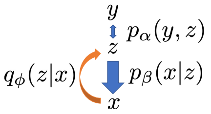
Figure 1: Graphical illustration of Symbol-Vector Coupling Energy-Based Model (SVEBM). $y$ is a symbolic one-hot vector, and $z$ is a dense continuous vector. $x$ is the observed example. $y$ and $z$ are coupled together through an EBM, $p_{\alpha}(y,z)$, in the latent space. Given $z$, $y$ and $x$ are independent, i.e., $z$ is sufficient for $y$, hence giving the generator model $p_{\beta}(x|z)$. The intractable posterior, $p_{\theta}(z|x)$ with $\theta=(\alpha,\beta)$, is approximated by a variational inference model, $q_{\phi}(z|x)$.

2 Model and learning

2.1 Model: symbol-vector coupling

Let $x$ be the observed text sequence. Let $z\in\mathbb{R}^{d}$ be the continuous latent vector. Let $y$ be the symbolic one-hot vector indicating one of $K$ categories. Our generative model is defined by

$$p_{\theta}(y,z,x)=p_{\alpha}(y,z)p_{\beta}(x|z),$$ (1)

where $p_{\alpha}(y,z)$ is the prior model with parameters $\alpha$, $p_{\beta}(x|z)$ is the top-down generation model with parameters $\beta$, and $\theta=(\alpha,\beta)$. Given $z$, $y$ and $x$ are independent, i.e., $z$ is sufficient for $y$.

The prior model $p_{\alpha}(y,z)$ is formulated as an energy-based model,

$$p_{\alpha}(y,z)=\frac{1}{Z_{\alpha}}\exp(\langle y,f_{\alpha}(z)\rangle)p_{0}(z),$$ (2)

where $p_{0}(z)$ is a reference distribution, assumed to be isotropic Gaussian (or uniform) non-informative prior of the conventional generator model. $f_{\alpha}(z)\in\mathbb{R}^{K}$ is parameterized by a small multi-layer perceptron. $Z_{\alpha}$ is the normalizing constant or partition function.

The energy term $\langle y,f_{\alpha}(z)\rangle$ in Equation (2) forms an associative memory that couples the symbol $y$ and the dense vector $z$. Given $z$,

$$p_{\alpha}(y|z)\propto\exp(\langle y,f_{\alpha}(z)\rangle),$$ (3)

i.e., a softmax classifier, where $f_{\alpha}(z)$ provides the $K$ logit scores for the $K$ categories. Marginally,

$$p_{\alpha}(z)=\frac{1}{Z_{\alpha}}\exp(F_{\alpha}(z))p_{0}(z),$$ (4)

where the marginal energy term

$$F_{\alpha}(z)=\log\sum_{y}\exp(\langle y,f_{\alpha}(z)\rangle),$$ (5)

i.e., the so-called log-sum-exponential form. The summation can be easily computed because we only need to sum over $K$ different values of the one-hot $y$.

The above prior model $p_{\alpha}(y,z)$ stands on a generation model $p_{\beta}(x|z)$. For text modeling, let $x=(x^{(t)},t=1,...,T)$ where $x^{(t)}$ is the $t$-th token. Following previous text VAE model (Bowman et al., 2016), we define $p_{\beta}(x|z)$ as a conditional autoregressive model,

$$p_{\beta}(x|z)=\prod_{t=1}^{T}p_{\beta}(x^{(t)}|x^{(1)},...,x^{(t-1)},z)$$ (6)

which is parameterized by a recurrent network with parameters $\beta$. See Figure 1 for a graphical illustration of our model.

2.2 Prior and posterior sampling: symbol-aware continuous vector computation

Sampling from the prior $p_{\alpha}(z)$ and the posterior $p_{\theta}(z|x)$ can be accomplished by Langevin dynamics. For prior sampling from $p_{\alpha}(z)$, Langevin dynamics iterates

$$z_{t+1}=z_{t}+s\nabla_{z}\log p_{\alpha}(z_{t})+\sqrt{2s}e_{t},$$ (7)

where $e_{t}\sim\mathcal{N}(0,I_{d})$, $s$ is the step size, and the gradient is computed by

$$\nabla_{z}\log p_{\alpha}(z) =\operatorname{\mathbb{E}}_{p_{\alpha}(y|z)}[\nabla_{z}\log p_{\alpha}(y,z)]$$

$$=\operatorname{\mathbb{E}}_{p_{\alpha}(y|z)}[\langle y,\nabla_{z}f_{\alpha}(z)\rangle],$$ (8)

where the gradient computation involves averaging $\nabla_{z}f_{\alpha}(z)$ over the softmax classification probabilities $p_{\alpha}(y|z)$ in Equation (3). Thus the sampling of the continuous dense vector $z$ is aware of the symbolic $y$.

Posterior sampling from $p_{\theta}(z|x)$ follows a similar scheme, where

$$\nabla_{z}\log p_{\theta}(z|x) =\operatorname{\mathbb{E}}_{p_{\alpha}(y|z)}[\langle y,\nabla_{z}f_{\alpha}(z)\rangle]$$

$$+\nabla_{z}\log p_{\beta}(x|z).$$ (9)

When the dynamics is reasoning about $x$ by sampling the dense continuous vector $z$ from $p_{\theta}(z|x)$, it is aware of the symbolic $y$ via the softmax $p_{\alpha}(y|z)$.

Thus $(y,z)$ forms a coupling between symbol and dense vector, which gives the name of our model, Symbol-Vector Coupling Energy-Based Model (SVEBM).

Pang et al. (2020a) proposes to use prior and posterior sampling for maximum likelihood learning. Due to the low-dimensionality of the latent space, MCMC sampling is affordable and mixes well.

2.3 Amortizing posterior sampling and variational learning

Comparing prior and posterior sampling, prior sampling is particularly affordable, because $f_{\alpha}(z)$ is a small network. In comparison, $\nabla_{z}\log p_{\beta}(x|z)$ in the posterior sampling requires back-propagation through the generator network, which can be more expensive. Therefore we shall amortize the posterior sampling from $p_{\theta}(z|x)$ by an inference network, and we continue to use MCMC for prior sampling.

Specifically, following VAE (Kingma & Welling, 2014), we recruit an inference network $q_{\phi}(z|x)$ to approximate the true posterior $p_{\theta}(z|x)$, in order to amortize posterior sampling. Following VAE, we learn the inference model $q_{\phi}(z|x)$ and the top-down model $p_{\theta}(y,z,x)$ in Equation (1) jointly.

For unlabeled $x$, the log-likelihood $\log p_{\theta}(x)$ is lower bounded by the evidence lower bound (ELBO),

$$\operatorname{\mathrm{ELBO}}(x|\theta,\phi)=\log p_{\theta}(x)-\operatorname{\mathbb{D}_{\rm KL}}(q_{\phi}(z|x)\|p_{\theta}(z|x))$$

$$=\operatorname{\mathbb{E}}_{q_{\phi}(z|x)}\left[\log p_{\beta}(x|z)\right]-\operatorname{\mathbb{D}_{\rm KL}}(q_{\phi}(z|x)\|p_{\alpha}(z)),$$ (10)

where $\operatorname{\mathbb{D}_{\rm KL}}$ denotes the Kullback-Leibler divergence.

For the prior model, the learning gradient is

$$\nabla_{\alpha}\operatorname{\mathrm{ELBO}}=\operatorname{\mathbb{E}}_{q_{\phi}(z|x)}[\nabla_{\alpha}F_{\alpha}(z)]-\operatorname{\mathbb{E}}_{p_{\alpha}(z)}[\nabla_{\alpha}F_{\alpha}(z)],$$ (11)

where $F_{\alpha}(z)$ is defined by (5), $\operatorname{\mathbb{E}}_{q_{\phi}(z|x)}$ is approximated by samples from the inference network, and $\operatorname{\mathbb{E}}_{p_{\alpha}(z)}$ is approximated by persistent MCMC samples from the prior.

Let $\psi=\{\beta,\phi\}$ collect the parameters of the inference (encoder) and generator (decoder) models. The learning gradients for the two models are

$$\nabla_{\psi}\operatorname{\mathrm{ELBO}}=\nabla_{\psi}\operatorname{\mathbb{E}}_{q_{\phi}(z|x)}[\log p_{\beta}(x|z)]$$

$$-\nabla_{\psi}\operatorname{\mathbb{D}_{\rm KL}}(q_{\phi}(z|x)\|p_{0}(z))+\nabla_{\psi}\operatorname{\mathbb{E}}_{q_{\phi(z|x)}}[F_{\alpha}(z)],$$ (12)

where $p_{0}(z)$ is the reference distribution in Equation (2), and $\operatorname{\mathbb{D}_{\rm KL}}(q_{\phi}(z|x)\|p_{0}(z))$ is tractable. The expectations in the other two terms are approximated by samples from the inference network $q_{\phi}(z|x)$ with reparametrization trick (Kingma & Welling, 2014). Compared to the original VAE, we only need to include the extra $F_{\alpha}(z)$ term in Equation (12), while $\log Z_{\alpha}$ is a constant that can be discarded. This expands the scope of VAE where the top-down model is a latent EBM.

As mentioned above, we shall not amortize the prior sampling from $p_{\alpha}(z)$ due to its simplicity. Sampling $p_{\alpha}(z)$ is only needed in the training stage, but is not required in the testing stage.

2.4 Two joint distributions

Let $q_{\rm data}(x)$ be the data distribution that generates $x$. For variational learning, we maximize the averaged ELBO: $\operatorname{\mathbb{E}}_{q_{\rm data}(x)}[\operatorname{\mathrm{ELBO}}(x|\theta,\phi)]$, where $\operatorname{\mathbb{E}}_{q_{\rm data}(x)}$ can be approximated by averaging over the training examples. Maximizing $\operatorname{\mathbb{E}}_{q_{\rm data}(x)}[\operatorname{\mathrm{ELBO}}(x|\theta,\phi)]$ over $(\theta,\phi)$ is equivalent to minimizing the following objective function over $(\theta,\phi)$

$$\operatorname{\mathbb{D}_{\rm KL}}(q_{\rm data}(x)\|p_{\theta}(x))+\operatorname{\mathbb{E}}_{q_{\rm data}(x)}[\operatorname{\mathbb{D}_{\rm KL}}(q_{\phi}(z|x)\|p_{\theta}(z|x))]$$

$$=\operatorname{\mathbb{D}_{\rm KL}}(q_{\rm data}(x)q_{\phi}(z|x)\|p_{\alpha}(z)p_{\beta}(x|z)).$$ (13)

The right hand side is the KL-divergence between two joint distributions: $Q_{\phi}(x,z)=q_{\rm data}(x)q_{\phi}(z|x)$, and $P_{\theta}(x,z)=p_{\alpha}(z)p_{\beta}(x|z)$. The reason we use notation $q$ for the data distribution $q_{\rm data}(x)$ is for notation consistency. Thus VAE can be considered as joint minimization of $\operatorname{\mathbb{D}_{\rm KL}}(Q_{\phi}\|P_{\theta})$ over $(\theta,\phi)$. Treating $(x,z)$ as the complete data, $Q_{\phi}$ can be considered the complete data distribution, while $P_{\theta}$ is the model distribution of the complete data.

For the distribution $Q_{\phi}(x,z)$, we can define the following quantities.

$$q_{\phi}(z)=\operatorname{\mathbb{E}}_{q_{\rm data}(x)}[q_{\phi}(z|x)]=\int Q_{\phi}(x,z)dx$$ (14)

is the aggregated posterior distribution and the marginal distribution of $z$ under $Q_{\phi}$. $\operatorname{\mathcal{H}}(z)=-\operatorname{\mathbb{E}}_{q_{\phi}(z)}[\log q_{\phi}(z)]$ is the entropy of the aggregated posterior $q_{\phi}(z)$.

$\operatorname{\mathcal{H}}(z|x)=-\operatorname{\mathbb{E}}_{Q_{\phi}(x,z)}[\log q_{\phi}(z|x)]$ is the conditional entropy of $z$ given $x$ under the variational inference distribution $q_{\phi}(z|x)$.

$$\operatorname{\mathcal{I}}(x,z)=\operatorname{\mathcal{H}}(z)-\operatorname{\mathcal{H}}(z|x)$$

$$=-\operatorname{\mathbb{E}}_{q_{\phi}(z)}[\log q_{\phi}(z)]+\operatorname{\mathbb{E}}_{Q_{\phi}(x,z)}[\log q_{\phi}(z|x)]$$ (15)

is the mutual information between $x$ and $z$ under $Q_{\phi}$.

It can be shown that the VAE objective in Equation (13) can be written as

$$\operatorname{\mathbb{D}_{\rm KL}} (Q_{\phi}(x,z)\|P_{\theta}(x,z))$$

$$=-\operatorname{\mathcal{H}}(x)-\operatorname{\mathbb{E}}_{Q_{\phi}(x,z)}[\log p_{\beta}(x|z)]$$

$$\quad+\operatorname{\mathcal{I}}(x,z)+\operatorname{\mathbb{D}_{\rm KL}}(q_{\phi}(z)\|p_{\alpha}(z)),$$ (16)

where $\operatorname{\mathcal{H}}(x)=-\operatorname{\mathbb{E}}_{q_{\rm data}(x)}[\log q_{\rm data}(x)]$ is the entropy of the data distribution and is fixed.

2.5 Information bottleneck

Due to the coupling of $y$ and $z$ (see Equations (2) and (3)), a learning objective with information bottleneck can be naturally developed as a simple modification of the VAE objective in Equations (13) and (16):

$$\operatorname{\mathcal{L}}(\theta,\phi) =\operatorname{\mathbb{D}_{\rm KL}}(Q_{\phi}(x,z)\|P_{\theta}(x,z))-\lambda\operatorname{\mathcal{I}}(z,y)$$ (17)

$$=-\operatorname{\mathcal{H}}(x)-\underbrace{\operatorname{\mathbb{E}}_{Q_{\phi}(x,z)}[\log p_{\beta}(x|z)]}_{\text{reconstruction}}$$ (18)

$$\quad+\underbrace{\operatorname{\mathbb{D}_{\rm KL}}(q_{\phi}(z)\|p_{\alpha}(z))}_{\text{EBM learning}}$$ (19)

$$\quad+\underbrace{\operatorname{\mathcal{I}}(x,z)-\lambda\operatorname{\mathcal{I}}(z,y)}_{\text{information bottleneck}},$$ (20)

where $\lambda\geq 0$ controls the trade-off between the compressivity of $z$ about $x$ and its expressivity to $y$. The mutual information between $z$ and $y$, $\operatorname{\mathcal{I}}(z,y)$, is defined as:

$$\operatorname{\mathcal{I}}(z,y) =\operatorname{\mathcal{H}}(y)-\operatorname{\mathcal{H}}(y|z)$$

$$=-\sum_{y}q(y)\log q(y)$$

$$\quad+\operatorname{\mathbb{E}}_{q_{\phi}(z)}\sum_{y}p_{\alpha}(y|z)\log p_{\alpha}(y|z),$$ (21)

where $q(y)=\operatorname{\mathbb{E}}_{q_{\phi}(z)}[p_{\alpha}(y|z)]$. $\operatorname{\mathcal{I}}(z,y)$, $\operatorname{\mathcal{H}}(y)$, and $\operatorname{\mathcal{H}}(y|z)$ are defined based on $Q(x,y,z)=q_{\rm data}(x)q_{\phi}(z|x)p_{\alpha}(y|z)$, where $p_{\alpha}(y|z)$ is softmax probability over $K$ categories in Equation (3).

In computing $\operatorname{\mathcal{I}}(z,y)$, we need to take expectation over $z$ under $q_{\phi}(z)=\operatorname{\mathbb{E}}_{q_{\rm data}(x)}[q_{\phi}(z|x)]$, which is approximated with a mini-batch of $x$ from $q_{\rm data}(x)$ and multiple samples of $z$ from $q_{\phi}(z|x)$ given each $x$.

The Lagrangian form of the classical information bottleneck objective (Tishby et al., 2000) is,

$$\min_{p_{\theta}(z|x)}[\operatorname{\mathcal{I}}(x,z|\theta)-\lambda\operatorname{\mathcal{I}}(z,y|\theta)].$$ (22)

Thus minimizing $\operatorname{\mathcal{L}}(\theta,\phi)$ (Equation (17)) includes minimizing a variational version (variational information bottleneck or VIB; Alemi et al. 2016) of Equation (22). We do not exactly minimize VIB due to the reconstruction term in Equation (18) that drives unsupervised learning, in contrast to supervised learning of VIB in Alemi et al. (2016).

We call the SVEBM learned with the objective incorporating information bottleneck (Equation (17)) as SVEBM-IB.

2.6 Labeled data

For a labeled example $(x,y)$, the log-likelihood can be decomposed into $\log p_{\theta}(x,y)=\log p_{\theta}(x)+\log p_{\theta}(y|x)$. The gradient of $\log p_{\theta}(x)$ and its ELBO can be computed in the same way as the unlabeled data described above.

$$p_{\theta}(y|x)=\operatorname{\mathbb{E}}_{p_{\theta}(z|x)}[p_{\alpha}(y|z)]\approx\operatorname{\mathbb{E}}_{q_{\phi}(z|x)}[p_{\alpha}(y|z)],$$ (23)

where $p_{\alpha}(y|z)$ is the softmax classifier defined by Equation (3), and $q_{\phi}(z|x)$ is the learned inference network. In practice, $\operatorname{\mathbb{E}}_{q_{\phi}(z|x)}[p_{\alpha}(y|z)]$ is further approximated by $p_{\alpha}(y|z=\mu_{\phi}(x))$ where $\mu_{\phi}(x)$ is the posterior mean of $q_{\phi}(z|x)$. We found using $\mu_{\phi}(x)$ gave better empirical performance than using multiple posterior samples.

For semi-supervised learning, we can combine the learning gradients from both unlabeled and labeled data.

2.7 Algorithm

The learning and sampling algorithm for SVEBM is described in Algorithm 1. Adding the respective gradients of $\operatorname{\mathcal{I}}(z,y)$ (Equation (21)) to Step 4 and Step 5 allows for learning SVEBM-IB.

Algorithm 1 Unsupervised and Semi-supervised Learning of Symbol-Vector Coupling Energy-Based Model.

  Input: Learning iterations $T$, learning rates $(\eta_{0},\eta_{1},\eta_{2})$, initial parameters $(\alpha_{0},\beta_{0},\phi_{0})$, observed unlabelled examples $\{x_{i}\}_{i=1}^{M}$, observed labelled examples $\{(x_{i},y_{i})\}_{i=M+1}^{M+N}$ (optional, needed only in semi-supervised learning), unlabelled and labelled batch sizes $(m,n)$, initializations of persistent chains $\{z_{i}^{-}\sim p_{0}(z)\}_{i=1}^{L}$, and number of Langevin dynamics steps $T_{LD}$.

  Output: $(\alpha_{T},\beta_{T},\phi_{T})$.

  for $t=0$ to $T-1$ do

     1. mini-batch: Sample unlabelled $\{x_{i}\}_{i=1}^{m}$ and labelled observed examples $\{x_{i},y_{i}\}_{i=m+1}^{m+n}$.

     2. prior sampling: For each unlabelled $x_{i}$, randomly pick and update a persistent chain $z_{i}^{-}$ by Langevin dynamics with target distribution $p_{\alpha}(z)$ for $T_{LD}$ steps.

     3. posterior sampling: For each $x_{i}$, sample $z_{i}^{+}\sim q_{\phi}(z|x_{i})$ using the inference network and reparameterization trick.

     4. unsupervised learning of prior model: $\alpha_{t+1}=\alpha_{t}+\eta_{0}\frac{1}{m}\sum_{i=1}^{m}[\nabla_{\alpha}F_{\alpha_{t}}(z_{i}^{+})-\nabla_{\alpha}F_{\alpha_{t}}(z_{i}^{-})]$.

     5. unsupervised learning of inference and generator models: $\psi_{t+1}=\psi_{t}+\eta_{1}\frac{1}{m}\sum_{i=1}^{m}[\nabla_{\psi}\log p_{\beta_{t}}(x_{i}|z_{i}^{+})-\nabla_{\psi}\operatorname{\mathbb{D}_{\rm KL}}(q_{\phi_{t}}(z|x_{i})\|p_{0}(z))+\nabla_{\psi}F_{\alpha_{t}}(z_{i}^{+})]$, with backpropagation through $z_{i}^{+}$ via reparametrization trick.

     if labeled examples $(x,y)$ are available then

        6. supervised learning of prior and inference models: Let $\gamma=(\alpha,\phi)$. $\gamma_{t+1}=\gamma_{t}+\eta_{2}\frac{1}{n}\sum_{i=m+1}^{m+n}$ $\nabla_{\gamma}\log p_{\alpha_{t}}(y_{i}|z_{i}=\mu_{\phi_{t}}(x_{i}))$.

     end if

  end for

3 Experiments

We present a set of experiments to assess (1) the quality of text generation, (2) the interpretability of text generation, and (3) semi-supervised classification of our proposed models, SVEBM and SVEBM-IB, on standard benchmarks. The proposed SVEBM is highly expressive for text modeling and demonstrate superior text generation quality and is able to discover meaningful latent labels when some supervision signal is available, as evidenced by good semi-supervised classification performance. SVEBM-IB not only enjoys the expressivity of SVEBM but also is able to discover meaningful labels in an unsupervised manner since the information bottleneck objective encourages the continuous latent variable, $z$, to keep sufficient information of the observed $x$ for the emergence of the label, $y$. Its advantage is still evident when supervised signal is provided.

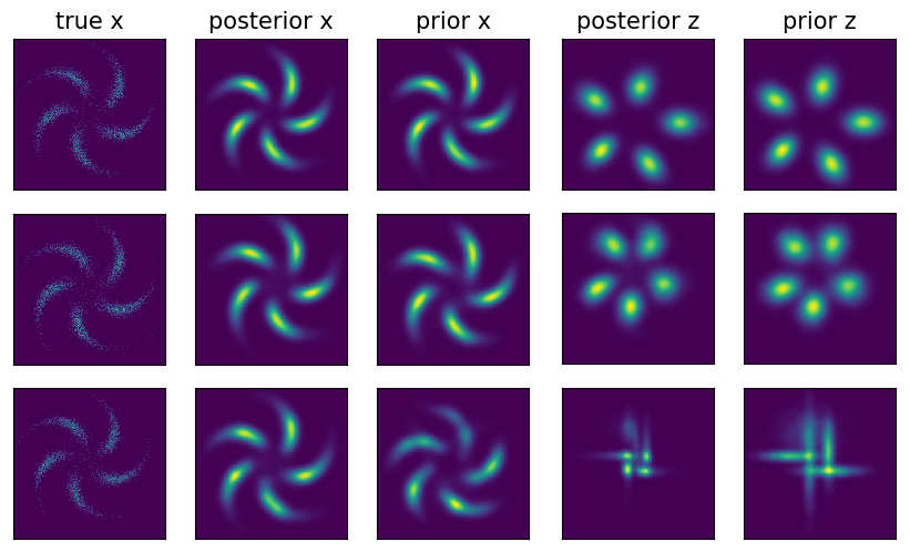
Figure 2: Evaluation on 2D synthetic data: a mixture of eight Gaussians (upper panel) and a pinwheel-shaped distribution (lower panel). In each panel, the first, second, and third row display densities learned by SVEBM-IB, SVEBM, and DGM-VAE, respectively.

3.1 Experiment settings

Generation quality is evaluated on the Penn Treebanks (Marcus et al. 1993, PTB) as pre-processed by Mikolov et al. (2010). Interpretability is first assessed on two dialog datasets, the Daily Dialog dataset (Li et al., 2017b) and the Stanford Multi-Domain Dialog (SMD) dataset (Eric et al., 2017). DD is a chat-oriented dataset and consists of $13,118$ daily conversations for English learner in a daily life. It provides human-annotated dialog actions and emotions for the utterances. SMD has $3,031$ human-Woz, task-oriented dialogues collected from three different domains (navigation, weather, and scheduling). We also evaluate generation interpretability of our models on sentiment control with Yelp reviews, as preprocessed by Li et al. (2018). It is on a larger scale than the aforementioned datasets, and contains $180,000$ negative reviews and $270,000$ positive reviews.

Our model is compared with the following baselines: (1) RNNLM (Mikolov et al., 2010), language model implemented with GRU (Cho et al., 2014); (2) AE (Vincent et al., 2010), deterministic autoencoder which has no regularization to the latent space; (3) DAE, autoencoder with a discrete latent space; (4) VAE (Kingma & Welling, 2014), the vanilla VAE with a continuous latent space and a Gaussian noise prior; (5) DVAE, VAE with a discrete latent space; (6) DI-VAE (Zhao et al., 2018b), a DVAE variant with a mutual information term between $x$ and $z$; (7) semi-VAE (Kingma et al., 2014), semi-supervised VAE model with independent discrete and continuous latent variables; (8) GM-VAE, VAE with discrete and continuous latent variables following a Gaussian mixture; (9) DGM-VAE (Shi et al., 2020), GM-VAE with a dispersion term which regularizes the modes of Gaussian mixture to avoid them collapsing into a single mode; (10) semi-VAE $+\operatorname{\mathcal{I}}(x,y)$, GM-VAE $+\operatorname{\mathcal{I}}(x,y)$, DGM-VAE $+\operatorname{\mathcal{I}}(x,y)$, are the same models as (7), (8), and (9) respectively, but with an mutual information term between $x$ and $y$ which can be computed since they all learn two separate inference networks for $y$ and $z$. To train these models involving discrete latent variables, one needs to deal with the non-differentiability of them in order to learn the inference network for $y$. In our models, we do not need a separate inference network for $y$, which can conveniently be inferred from $z$ given the inferred $z$ (see Equation 3), and have no need to sample from the discrete variable in training.

The encoder and decoder in all models are implemented with a single-layer GRU with hidden size 512. The dimensions for the continuous vector are $40$, $32$, $32$, and $40$ for PTB, DD, SMD and Yelp, respectively. The dimensions for the discrete variable are $20$ for PTB, $125$ for DD, $125$ for SMD, and $2$ for Yelp. $\lambda$ in information bottleneck (see Equation 17) that controls the trade-off between compressivity of $z$ about $x$ and its expressivity to $y$ is not heavily tuned and set to $50$ for all experiments. Our implementation is available at https://github.com/bpucla/ibebm.git.

3.2 2D synthetic data

We first evaluate our models on 2-dimensional synthetic datasets for direct visual inspection. They are compared to the best performing baseline in prior works, DGM-VAE $+\operatorname{\mathcal{I}}(x,y)$ (Shi et al., 2020). The results are displayed in Figure 2. In each row, true x indicates the true data distribution $q_{\rm data}(x)$; posterior x indicates the KDE (kernel density estimation) distribution of $x$ based on $z$ samples from its posterior $q_{\phi}(z|x)$; prior x indicates the KDE of $p_{\theta}(x)=\int p_{\beta}(x|z)p_{\alpha}(z)dz$, based on $z$ samples from the learned EBM prior, $p_{\alpha}(z)$; posterior z indicates the KDE of the aggregate posterior, $q_{\phi}(z)=\int q_{\rm data}(x)q_{\phi}(z|x)dx$; prior z indicates the KDE of the learned EBM prior, $p_{\alpha}(z)$.

It is clear that our proposed models, SVEBM and SVEBM-IB model the data well in terms of both posterior x and prior x. In contrast, although DGM-VAE reconstructs the data well but the learned generator $p_{\theta}(x)$ tend to miss some modes. The learned prior $p_{\theta}(z)$ in SVEBM and SVEBM-IB shows the same number of modes as the data distribution and manifests a clear structure. Thus, the well-structured latent space is able to guide the generation of $x$. By comparison, although DGM-VAE shows some structure in the latent space, the structure is less clear than that of our model. It is also worth noting that SVEBM performs similarly as SVEBM-IB, and thus the symbol-vector coupling per se, without the information bottleneck, is able to capture the latent space structure of relatively simple synthetic data.

3.3 Language generation

We evaluate the quality of text generation on PTB and report four metrics to assess the generation performance: reverse perplexity (rPPL; Zhao et al. 2018a), BELU (Papineni et al., 2002), word-level KL divergence (wKL), and negative log-likelihood (NLL). Reverse perplexity is the perplexity of ground-truth test set computed under a language model trained with generated data. Lower rPPL indicates that the generated sentences have higher diversity and fluency. We recruit ASGD Weight-Dropped LSTM (Merity et al., 2018), a well-performed and popular language model, to compute rPPL. The synthesized sentences are sampled with $z$ samples from the learned latent space EBM prior, $p_{\alpha}(z)$. The BLEU score is computed between the input and reconstructed sentences and measures the reconstruction quality. Word-level KL divergence between the word frequencies of training data and synthesized data reflects the generation quality. Negative log-likelihood  measures the general model fit to the data. These metrics are evaluated on the test set of PTB, except wKL, which is evaluated on the training set.

The results are summarised in Table 1. Compared to previous models with (1) only continuous latent variables, (2) only discrete latent variables, and (3) both discrete and continuous latent variables, the coupling of discrete and continuous latent variables in our models through an EBM is more expressive. The proposed models, SVEBM and SVEBM-IB, demonstrate better reconstruction (higher BLEU) and higher model fit (lower NLL) than all baseline models except AE. Its sole objective is to reconstruct the input and thus it can reconstruct sentences well but cannot generate diverse sentences.

The expressivity of our models not only allows for capturing the data distribution well but also enables them to generate sentences of high-quality. As indicated by the lowest rPPL, our models improve over these strong baselines on fluency and diversity of generated text. Moreover, the lowest wKL of our models indicate that the word distribution of the generated sentences by our models is most consistent with that of the data.

It is worth noting that SVEBM and SVEBM-IB have close performance on language modeling and text generation. Thus the mutual information term does not lessen the model expressivity.

Model	rPPL↓	BLEU↑	wKL↓	NLL↓
Test Set	-	100.0	0.14	-
RNN-LM	-	-	-	101.21
AE	730.81	10.88	0.58	-
VAE	686.18	3.12	0.50	100.85
DAE	797.17	3.93	0.58	-
DVAE	744.07	1.56	0.55	101.07
DI-VAE	310.29	4.53	0.24	108.90
semi-VAE	494.52	2.71	0.43	100.67
semi-VAE $+\operatorname{\mathcal{I}}(x,y)$	260.28	5.08	0.20	107.30
GM-VAE	983.50	2.34	0.72	99.44
GM-VAE $+\operatorname{\mathcal{I}}(x,y)$	287.07	6.26	0.25	103.16
DGM-VAE	257.68	8.17	0.19	104.26
DGM-VAE $+\operatorname{\mathcal{I}}(x,y)$	247.37	8.67	0.18	105.73
SVEBM	180.71	9.54	0.17	95.02
SVEBM-IB	177.59	9.47	0.16	94.68

Table 1: Results of language generation on PTB.

3.4 Interpretable generation

We next turn to evaluate our models on the interpretabiliy of text generation.

Unconditional text generation.  The dialogues are flattened for unconditional modeling. Utterances in DD are annotated with action and emotion labels. The generation interpretability is assessed through the ability to unsupervisedly capture the utterance attributes of DD. The label, $y$, of an utterance, $x$, is inferred from the posterior distribution, $p_{\theta}(y|x)$ (see Equation 23). In particular, we take $y={\rm argmax}_{k}p_{\theta}(y=k|x)$ as the inferred label. As in Zhao et al. (2018b) and Shi et al. (2020), we recruit homogeneity to evaluate the consistency between groud-truth action and emotion labels and those inferred from our models. Table 2 displays the results of our models and baselines. Without the mutual information term to encourage $z$ to retain sufficient information for label emergence, the continuous latent variables in SVEBM appears to mostly encode information for reconstructing $x$ and performs the best on sentence reconstruction. However, the encoded information in $z$ is not sufficient for the model to discover interpretable labels and demonstrates low homogeneity scores. In contrast, SVEBM-IB is designed to encourage $z$ to encode information for an interpretable latent space and greatly improve the interpretability of text generation over SVEBM and models from prior works, as evidenced in the highest homogeneity scores on action and emotion labels.

Model	MI↑	BLEU↑	Action↑	Emotion↑
DI-VAE	1.20	3.05	0.18	0.09
semi-VAE	0.03	4.06	0.02	0.08
semi-VAE $+\operatorname{\mathcal{I}}(x,y)$	1.21	3.69	0.21	0.14
GM-VAE	0.00	2.03	0.08	0.02
GM-VAE $+\operatorname{\mathcal{I}}(x,y)$	1.41	2.96	0.19	0.09
DGM-VAE	0.53	7.63	0.11	0.09
DGM-VAE $+\operatorname{\mathcal{I}}(x,y)$	1.32	7.39	0.23	0.16
SVEBM	0.01	11.16	0.03	0.01
SVEBM-IB	2.42	10.04	0.59	0.56

Table 2: Results of interpretable language generation on DD. Mutual information (MI), BLEU and homogeneity with actions and emotions are shown.

Conditional text generation.  We then evaluate SVEBM-IB on dialog generation with SMD. BELU and three word-embedding-based topic similarity metrics, embedding average, embedding extrema and embedding greedy (Mitchell & Lapata, 2008; Forgues et al., 2014; Rus & Lintean, 2012), are employed to evaluate the quality of generated responses. The evaluation results are summarized in Table 3. SVEBM-IB outperforms all baselines on all metrics, indicating the high-quality of the generated dialog utterances.

SMD does not have human annotated action labels. We thus assess SVEBM-IB qualitatively. Table 4 shows dialog actions discovered by it and their corresponding utterances. The utterances with the same action are assigned with the same latent code ($y$) by our model. Table 5 displays dialog responses generated with different values of $y$ given the same context. It shows that SVEBM-IB is able to generate interpretable utterances given the context.

Model	BLEU↑	Average↑	Extrema↑	Greedy↑
DI-VAE	7.06	76.17	43.98	60.92
DGM-VAE $+\operatorname{\mathcal{I}}(x,y)$	10.16	78.93	48.14	64.87
SVEBM-IB	12.01	80.88	51.35	67.12

Table 3: Dialog evaluation results on SMD with four metrics: BLEU, average, extrema and greedy word embedding based similarity.

Action	Inform-weather
Utterance	Next week it will rain on Saturday in Los Angeles
	It will be between 20-30F in Alhambra on Friday.
	It won’t be overcast or cloudy at all this week in Carson
Action	Request-traffic/route
Utterance	Which one is the quickest, is there any traffic?
	Is that route avoiding heavy traffic?
	Is there an alternate route with no traffic?

Table 4: Sample actions and corresponding utterances discovered by SVEBM-IB on SMD.

Context	Sys: What city do you want to hear the forecast for?
	User: Mountain View
Predict	Today in Mountain View is gonna be overcast, with low of 60F
	and high of 80F.
	What would you like to know about the weather for Mountain View?
Context	User: Where is the closest tea house?
	Sys: Peets Coffee also serves tea. They are 2 miles away
	at 9981 Archuleta Ave.
Predict	OK, please give me an address and directions via the shortest distance.
	Thanks!

Table 5: Dialog cases on SMD, which are generated by sampling dialog utterance $x$ with different values of $y$.

Sentence attribute control.   We evaluate our model’s ability to control sentence attribute. In particular, it is measured by the accuracy of generating sentences with a designated sentiment. This experiment is conducted with the Yelp reviews. Sentences are generated given the discrete latent code $y$. A pre-trained classifier is used to determine which sentiment the generated sentence has. The pre-trained classifier has an accuracy of $98.5\%$ on the testing data, and thus is able to accurately evaluate a sentence’s sentiment. There are multiple ways to cluster the reviews into two categories or in other words the sentiment attribute is not identifiable. Thus the models are trained with sentiment supervision. In addition to DGM-VAE $+\operatorname{\mathcal{I}}(x,y)$, we also compare our model to text conditional GAN (Subramanian et al., 2018).

The quantitative results are summarized in Table 6. All models have similar high accuracies of generating positive reviews. The accuracies of generating negative reviews are however lower. This might be because of the unbalanced proportions of positive and negative reviews in the training data. Our model is able to generate negative reviews with a much higher accuracy than the baselines, and has the highest overall accuracy of sentiment control. Some generated samples with a given sentiment are displayed in Table 7.

Model	Overall↑	Positive↑	Negative↑
DGM-VAE $+\operatorname{\mathcal{I}}(x,y)$	64.7%	95.3%	34.0%
CGAN	76.8%	94.9%	58.6%
SVEBM-IB	90.1%	95.1%	85.2%

Table 6: Accuracy of sentence attribute control on Yelp.

Positive	The staff is very friendly and the food is great.
	The best breakfast burritos in the valley.
	So I just had a great experience at this hotel.
	It’s a great place to get the food and service.
	I would definitely recommend this place for your customers.
Negative	I have never had such a bad experience.
	The service was very poor.
	I wouldn’t be returning to this place.
	Slowest service I’ve ever experienced.
	The food isn’t worth the price.

Table 7: Generated positive and negative reviews with SVEBM-IB trained on Yelp.

3.5 Semi-supervised classification

We next evaluate our models with supervised signal partially given to see if they can effectively use provided labels. Due to the flexible formulation of our model, they can be naturally extended to semi-supervised settings (Section 2.6).

In this experiment, we switch from neural sequence models used in previous experiments to neural document models (Miao et al., 2016; Card et al., 2018) to validate the wide applicability of our proposed models. Neural document models use bag-of-words representations. Each document is a vector of vocabulary size and each element represents a word’s occurring frequency in the document, modeled by a multinominal distribution. Due to the non-autoregressive nature of neural document model, it involves lower time complexity and is more suitable for low resources settings than neural sequence model.

We compare our models to VAMPIRE (Gururangan et al., 2019), a recent VAE-based semi-supervised learning model for text, and its more recent variants (Hard EM and CatVAE in Table 8) (Jin et al., 2020) that improve over VAMPIRE. Other baselines are (1) supervised learning with randomly initialized embedding; (2) supervised learning with Glove embedding pretrained on $840$ billion words (Glove-OD); (3) supervised learning with Glove embedding trained on in-domain unlabeled data (Glove-ID); (4) self-training where a model is trained with labeled data and the predicted labels with high confidence is added to the labeled training set. The models are evaluated on AGNews (Zhang et al., 2015) with varied number of labeled data. It is a popular benchmark for text classification and contains $127,600$ documents from $4$ classes.

The results are summarized in Table 8. SVEBM has reasonable performance in the semi-supervised setting where partial supervision signal is available. SVEBM performs better or on par with Glove-OD, which has access to a large amount of out-of-domain data, and VAMPIRE, the model specifically designed for text semi-supervised learning. It suggests that SVEBM is effective in using labeled data. These results support the validity of the proposed symbol-vector coupling formation for learning a well-structured latent space. SVEBM-IB outperforms all baselines especially when the number of labels is limited ($200$ or $500$ labels), clearly indicating the effectiveness of the information bottleneck for inducing structured latent space.

Model	200	500	2500	10000
Supervised	68.8	77.3	84.4	87.5
Self-training	77.3	81.3	84.8	87.7
Glove-ID	70.4	78.0	84.1	87.1
Glove-OD	68.8	78.8	85.3	88.0
VAMPIRE	82.9	84.5	85.8	87.7
Hard EM	83.9	84.6	85.1	86.9
CatVAE	84.6	85.7	86.3	87.5
SVEBM	84.5	84.7	86.0	88.1
SVEBM-IB	86.4	87.4	87.9	88.6

Table 8: Semi-supervised classification accuracy on AGNews with varied number of labeled data.

4 Related work and discussions

Text generation.  VAE is a prominent generative model (Kingma & Welling, 2014; Rezende et al., 2014). It is first applied to text modeling by Bowman et al. (2016). Following works apply VAE to a wide variety of challenging text generation problems such as dialog generation (Serban et al., 2016, 2017; Zhao et al., 2017, 2018b), machine translation (Zhang et al., 2016), text summarization (Li et al., 2017a), and paraphrase generation (Gupta et al., 2018). Also, a large number of following works have endeavored to improve language modeling and text generation with VAE by addressing issues like posterior collapse (Zhao et al., 2018a; Li et al., 2019; Fu et al., 2019; He et al., 2019).

Recently, Zhao et al. (2018b) and Shi et al. (2020) explore the interpretability of text generation with VAEs. While the model in Zhao et al. (2018b) has a discrete latent space, in Shi et al. (2020) the model contains both discrete ($y$) and continuous ($z$) variables which follow Gaussian mixture. Similarly, we use both discrete and continuous variables. But they are coupled together through an EBM which is more expressive than Gaussian mixture as a prior model, as illustrated in our experiments where both SVEBM and SVEBM-IB outperform the models from Shi et al. (2020) on language modeling and text generation. Moreover, our coupling formulation makes the mutual information between $z$ and $y$ can be easily computed without the need to train and tune an additional auxiliary inference network for $y$ or deal with the non-diffierentibility with regard to it, while Shi et al. (2020) recruits an auxiliary network to infer $y$ conditional on $x$ to compute their mutual information . Kingma et al. (2014) also proposes a VAE with both discrete and continuous latent variables but they are independent and $z$ follows an non-informative prior. These designs make it less powerful than ours in both generation quality and interpretability as evidenced in our experiments.

Energy-based model.  Recent works (Xie et al., 2016; Nijkamp et al., 2019; Han et al., 2020) demonstrate the effectiveness of EBMs in modeling complex dependency. Pang et al. (2020a) proposes to learn an EBM in the latent space as a prior model for the continuous latent vector, which greatly improves the model expressivity and demonstrates strong performance on text, image, molecule generation, and trajectory generation (Pang et al., 2020b, 2021). We also recruit an EBM as the prior model but this EBM couples a continuous vector and a discrete one, allowing for learning a more structured latent space, rendering generation interpretable, and admitting classification. In addition, the prior work uses MCMC for posterior inference but we recruits an inference network, $q_{\phi}(z|x)$, so that we can efficiently optimize over it, which is necessary for learning with the information bottleneck principle. Thus, this design admits a natural extension based on information bottleneck.

Grathwohl et al. (2019) proposes the joint energy-based model (JEM) which is a classifier based EBM. Our model moves JEM to latent space. This brings two benefits. (1) Learning EBM in the data space usually involves expensive MCMC sampling. Our EBM is built in the latent space which has a much lower dimension and thus the sampling is much faster and has better mixing. (2) It is not straightforward to apply JEM to text data since it uses gradient-based sampling while the data space of text is non-differentiable.

Information bottleneck.  Information bottleneck proposed by Tishby et al. (2000) is an appealing principle to find good representations that trade-offs between the minimality of the representation and its sufficiency for predicting labels. Computing mutual information involved in applying this principle is however often computationally challenging. Alemi et al. (2016) proposes a variational approach to reduce the computation complexity and uses it train supervised classifiers. In contrast, the information bottleneck in our model is embedded in a generative model and learned in an unsupervised manner.

5 Conclusion

In this work, we formulate a latent space EBM which couples a dense vector for generation and a symbolic vector for interpretability and classification. The symbol or category can be inferred from the observed example based on the dense vector. The latent space EBM is used as the prior model for text generation model. The symbol-vector coupling, the generator network, and the inference network are learned jointly by maximizing the variational lower bound of the log-likelihood. Our model can be learned in unsupervised setting and the learning can be naturally extended to semi-supervised setting. The coupling formulation and the variational learning together naturally admit an incorporation of information bottleneck which encourages the continuous latent vector to extract information from the observed example that is informative of the underlying symbol. Our experiments demonstrate that the proposed model learns a well-structured and meaningful latent space, which (1) guides the top-down generator to generate text with high quality and interpretability, and (2) can be leveraged to effectively and accurately classify text.

References

- Alemi et al. (2016) Alemi, A. A., Fischer, I., Dillon, J. V., and Murphy, K. Deep variational information bottleneck. arXiv preprint arXiv:1612.00410, 2016.
- Aneja et al. (2020) Aneja, J., Schwing, A., Kautz, J., and Vahdat, A. Ncp-vae: Variational autoencoders with noise contrastive priors, 2020.
- Bowman et al. (2016) Bowman, S. R., Vilnis, L., Vinyals, O., Dai, A., Jozefowicz, R., and Bengio, S. Generating sentences from a continuous space. In Proceedings of The 20th SIGNLL Conference on Computational Natural Language Learning, pp. 10–21, Berlin, Germany, August 2016. Association for Computational Linguistics. doi: 10.18653/v1/K16-1002. URL https://www.aclweb.org/anthology/K16-1002.
- Brown et al. (1993) Brown, P. F., Della Pietra, S. A., Della Pietra, V. J., and Mercer, R. L. The mathematics of statistical machine translation: Parameter estimation. Computational linguistics, 19(2):263–311, 1993.
- Burda et al. (2015) Burda, Y., Grosse, R., and Salakhutdinov, R. Importance weighted autoencoders. arXiv preprint arXiv:1509.00519, 2015.
- Card et al. (2018) Card, D., Tan, C., and Smith, N. A. Neural models for documents with metadata. In Proceedings of the 56th Annual Meeting of the Association for Computational Linguistics (Volume 1: Long Papers), pp. 2031–2040, 2018.
- Cho et al. (2014) Cho, K., van Merriënboer, B., Gulcehre, C., Bahdanau, D., Bougares, F., Schwenk, H., and Bengio, Y. Learning phrase representations using rnn encoder–decoder for statistical machine translation. In Proceedings of the 2014 Conference on Empirical Methods in Natural Language Processing (EMNLP), pp. 1724–1734, 2014.
- Eric et al. (2017) Eric, M., Krishnan, L., Charette, F., and Manning, C. D. Key-value retrieval networks for task-oriented dialogue. Annual Meeting of the Special Interest Group on Discourse and Dialogue, pp. 37–49, 2017.
- Forgues et al. (2014) Forgues, G., Pineau, J., Larchevêque, J.-M., and Tremblay, R. Bootstrapping dialog systems with word embeddings. In NIPS, Modern Machine Learning and Natural Language Processing Workshop, volume 2, 2014.
- Fu et al. (2019) Fu, H., Li, C., Liu, X., Gao, J., Celikyilmaz, A., and Carin, L. Cyclical annealing schedule: A simple approach to mitigating KL vanishing. In Proceedings of the 2019 Conference of the North American Chapter of the Association for Computational Linguistics: Human Language Technologies, Volume 1 (Long and Short Papers), pp. 240–250, Minneapolis, Minnesota, June 2019. Association for Computational Linguistics. doi: 10.18653/v1/N19-1021. URL https://www.aclweb.org/anthology/N19-1021.
- Grathwohl et al. (2019) Grathwohl, W., Wang, K.-C., Jacobsen, J.-H., Duvenaud, D., Norouzi, M., and Swersky, K. Your classifier is secretly an energy based model and you should treat it like one. In International Conference on Learning Representations, 2019.
- Gupta et al. (2018) Gupta, A., Agarwal, A., Singh, P., and Rai, P. A deep generative framework for paraphrase generation. In Proceedings of the AAAI Conference on Artificial Intelligence, volume 32, 2018.
- Gururangan et al. (2019) Gururangan, S., Dang, T., Card, D., and Smith, N. A. Variational pretraining for semi-supervised text classification. In Proceedings of the 57th Annual Meeting of the Association for Computational Linguistics, pp. 5880–5894, 2019.
- Han et al. (2020) Han, T., Nijkamp, E., Zhou, L., Pang, B., Zhu, S.-C., and Wu, Y. N. Joint training of variational auto-encoder and latent energy-based model. In The IEEE/CVF Conference on Computer Vision and Pattern Recognition (CVPR), June 2020.
- He et al. (2019) He, J., Spokoyny, D., Neubig, G., and Berg-Kirkpatrick, T. Lagging inference networks and posterior collapse in variational autoencoders. In Proceedings of ICLR, 2019.
- Jin et al. (2020) Jin, S., Wiseman, S., Stratos, K., and Livescu, K. Discrete latent variable representations for low-resource text classification. In Proceedings of the 58th Annual Meeting of the Association for Computational Linguistics, pp. 4831–4842, Online, July 2020. Association for Computational Linguistics. doi: 10.18653/v1/2020.acl-main.437. URL https://www.aclweb.org/anthology/2020.acl-main.437.
- Kingma & Welling (2014) Kingma, D. P. and Welling, M. Auto-encoding variational bayes. In 2nd International Conference on Learning Representations, ICLR 2014, Banff, AB, Canada, April 14-16, 2014, Conference Track Proceedings, 2014. URL http://arxiv.org/abs/1312.6114.
- Kingma et al. (2014) Kingma, D. P., Mohamed, S., Rezende, D. J., and Welling, M. Semi-supervised learning with deep generative models. In Advances in neural information processing systems, pp. 3581–3589, 2014.
- Li et al. (2019) Li, B., He, J., Neubig, G., Berg-Kirkpatrick, T., and Yang, Y. A surprisingly effective fix for deep latent variable modeling of text. In Proceedings of the 2019 Conference on Empirical Methods in Natural Language Processing and the 9th International Joint Conference on Natural Language Processing (EMNLP-IJCNLP), pp. 3603–3614, Hong Kong, China, November 2019. Association for Computational Linguistics. doi: 10.18653/v1/D19-1370. URL https://www.aclweb.org/anthology/D19-1370.
- Li et al. (2018) Li, J., Jia, R., He, H., and Liang, P. Delete, retrieve, generate: a simple approach to sentiment and style transfer. In Proceedings of the 2018 Conference of the North American Chapter of the Association for Computational Linguistics: Human Language Technologies, Volume 1 (Long Papers), pp. 1865–1874, New Orleans, Louisiana, June 2018. Association for Computational Linguistics. doi: 10.18653/v1/N18-1169. URL https://www.aclweb.org/anthology/N18-1169.
- Li et al. (2017a) Li, P., Lam, W., Bing, L., and Wang, Z. Deep recurrent generative decoder for abstractive text summarization. In Proceedings of the 2017 Conference on Empirical Methods in Natural Language Processing, pp. 2091–2100, 2017a.
- Li et al. (2017b) Li, Y., Su, H., Shen, X., Li, W., Cao, Z., and Niu, S. Dailydialog: A manually labelled multi-turn dialogue dataset. International Joint Conference on Natural Language Processing, 1:986–995, 2017b.
- Marcus et al. (1993) Marcus, M. P., Marcinkiewicz, M. A., and Santorini, B. Building a large annotated corpus of english: The penn treebank. Comput. Linguist., 19(2):313–330, June 1993. ISSN 0891-2017. URL http://dl.acm.org/citation.cfm?id=972470.972475.
- Merity et al. (2018) Merity, S., Keskar, N. S., and Socher, R. Regularizing and optimizing lstm language models. In International Conference on Learning Representations, 2018.
- Miao et al. (2016) Miao, Y., Yu, L., and Blunsom, P. Neural variational inference for text processing. In International conference on machine learning, pp. 1727–1736. PMLR, 2016.
- Mikolov et al. (2010) Mikolov, T., Karafiát, M., Burget, L., Černockỳ, J., and Khudanpur, S. Recurrent neural network based language model. In Eleventh annual conference of the international speech communication association, 2010.
- Mitchell & Lapata (2008) Mitchell, J. and Lapata, M. Vector-based models of semantic composition. proceedings of ACL-08: HLT, pp. 236–244, 2008.
- Nijkamp et al. (2019) Nijkamp, E., Hill, M., Zhu, S.-C., and Wu, Y. N. Learning non-convergent non-persistent short-run MCMC toward energy-based model. Advances in Neural Information Processing Systems 33: Annual Conference on Neural Information Processing Systems 2019, NeurIPS 2019, 8-14 December 2019, Vancouver, Canada, 2019.
- Pang et al. (2020a) Pang, B., Han, T., Nijkamp, E., Zhu, S.-C., and Wu, Y. N. Learning latent space energy-based prior model. Advances in Neural Information Processing Systems, 33, 2020a.
- Pang et al. (2020b) Pang, B., Han, T., and Wu, Y. N. Learning latent space energy-based prior model for molecule generation. arXiv preprint arXiv:2010.09351, 2020b.
- Pang et al. (2021) Pang, B., Zhao, T., Xie, X., and Wu, Y. N. Trajectory prediction with latent belief energy-based model. arXiv preprint arXiv:2104.03086, 2021.
- Papineni et al. (2002) Papineni, K., Roukos, S., Ward, T., and Zhu, W.-J. Bleu: a method for automatic evaluation of machine translation. In Proceedings of the 40th annual meeting of the Association for Computational Linguistics, pp. 311–318, 2002.
- Rezende et al. (2014) Rezende, D. J., Mohamed, S., and Wierstra, D. Stochastic backpropagation and approximate inference in deep generative models. In Proceedings of the 31th International Conference on Machine Learning, ICML 2014, Beijing, China, 21-26 June 2014, pp. 1278–1286, 2014. URL http://proceedings.mlr.press/v32/rezende14.html.
- Rus & Lintean (2012) Rus, V. and Lintean, M. A comparison of greedy and optimal assessment of natural language student input using word-to-word similarity metrics. In Proceedings of the Seventh Workshop on Building Educational Applications Using NLP, pp. 157–162. Association for Computational Linguistics, 2012.
- Serban et al. (2016) Serban, I., Sordoni, A., Bengio, Y., Courville, A., and Pineau, J. Building end-to-end dialogue systems using generative hierarchical neural network models. In Proceedings of the AAAI Conference on Artificial Intelligence, volume 30, 2016.
- Serban et al. (2017) Serban, I., Sordoni, A., Lowe, R., Charlin, L., Pineau, J., Courville, A., and Bengio, Y. A hierarchical latent variable encoder-decoder model for generating dialogues. In Proceedings of the AAAI Conference on Artificial Intelligence, volume 31, 2017.
- Shi et al. (2020) Shi, W., Zhou, H., Miao, N., and Li, L. Dispersed exponential family mixture vaes for interpretable text generation. In International Conference on Machine Learning, pp. 8840–8851. PMLR, 2020.
- Subramanian et al. (2018) Subramanian, S., Rajeswar, S., Sordoni, A., Trischler, A., Courville, A., and Pal, C. Towards text generation with adversarially learned neural outlines. In Proceedings of the 32nd International Conference on Neural Information Processing Systems, pp. 7562–7574, 2018.
- Tishby et al. (2000) Tishby, N., Pereira, F. C., and Bialek, W. The information bottleneck method. arXiv preprint physics/0004057, 2000.
- Vincent et al. (2010) Vincent, P., Larochelle, H., Lajoie, I., Bengio, Y., and Manzagol, P. A. Stacked denoising autoencoders: Learning useful representations in a deep network with a local denoising criterion. Journal of Machine Learning Research, 11(12):3371–3408, 2010.
- Wang et al. (2019) Wang, W., Gan, Z., Xu, H., Zhang, R., Wang, G., Shen, D., Chen, C., and Carin, L. Topic-guided variational auto-encoder for text generation. In Proceedings of the 2019 Conference of the North American Chapter of the Association for Computational Linguistics: Human Language Technologies, Volume 1 (Long and Short Papers), pp. 166–177, 2019.
- Xie et al. (2016) Xie, J., Lu, Y., Zhu, S., and Wu, Y. N. A theory of generative convnet. In Proceedings of the 33nd International Conference on Machine Learning, ICML 2016, New York City, NY, USA, June 19-24, 2016, pp. 2635–2644, 2016. URL http://proceedings.mlr.press/v48/xiec16.html.
- Young et al. (2013) Young, S., Gašić, M., Thomson, B., and Williams, J. D. Pomdp-based statistical spoken dialog systems: A review. Proceedings of the IEEE, 101(5):1160–1179, 2013.
- Zhang et al. (2016) Zhang, B., Xiong, D., Su, J., Duan, H., and Zhang, M. Variational neural machine translation. In Proceedings of the 2016 Conference on Empirical Methods in Natural Language Processing, pp. 521–530, Austin, Texas, November 2016. Association for Computational Linguistics. doi: 10.18653/v1/D16-1050. URL https://www.aclweb.org/anthology/D16-1050.
- Zhang et al. (2015) Zhang, X., Zhao, J., and LeCun, Y. Character-level convolutional networks for text classification. In Advances in neural information processing systems, pp. 649–657, 2015.
- Zhao et al. (2018a) Zhao, J., Kim, Y., Zhang, K., Rush, A., and LeCun, Y. Adversarially regularized autoencoders. In International Conference on Machine Learning, pp. 5902–5911, 2018a.
- Zhao et al. (2017) Zhao, T., Zhao, R., and Eskenazi, M. Learning discourse-level diversity for neural dialog models using conditional variational autoencoders. In Proceedings of the 55th Annual Meeting of the Association for Computational Linguistics (Volume 1: Long Papers), pp. 654–664, 2017.
- Zhao et al. (2018b) Zhao, T., Lee, K., and Eskenazi, M. Unsupervised discrete sentence representation learning for interpretable neural dialog generation. In Proceedings of the 56th Annual Meeting of the Association for Computational Linguistics (Volume 1: Long Papers), pp. 1098–1107, 2018b.