PULSEE: A software for the quantum simulation of an extensive set of magnetic resonance observables

Abstract

We present an open-source software for the simulation of observables in magnetic resonance experiments, including nuclear magnetic/quadrupole resonance NMR/NQR and electron spin resonance (ESR)), developed to assist experimental research in the design of new strategies for the investigation of fundamental quantum properties of materials, as inspired by magnetic resonance protocols that emerged in the context of quantum information science (QIS). The package introduced here enables the simulation of both standard NMR spectroscopic observables and the time-evolution of an interacting single-spin system subject to complex pulse sequences, i.e. quantum gates. The main purpose of this software is to facilitate in the development of much needed novel NMR-based probes of emergent quantum orders, which can be elusive to standard experimental probes. The software is based on a quantum mechanical description of nuclear spin dynamics in NMR/NQR experiments and has been widely tested on available theoretical and experimental results. Moreover, the structure of the software allows for basic experiments to easily be generalized to more sophisticated ones, as it includes all the libraries required for the numerical simulation of generic spin systems. In order to make the program easily accessible to a large user base, we developed a user-friendly graphical interface, Jupyter notebooks, and fully-detailed documentation. Lastly, we portray several examples of the execution of the code that illustrate the potential of a novel NMR paradigm, inspired by QIS, for efficient investigation of emergent phases in strongly correlated materials.

PROGRAM SUMMARY/NEW VERSION PROGRAM SUMMARY

Program Title: PULSEE (Program for the simULation of nuclear Spin Ensemble Evolution)
CPC Library link to program files: (to be added by Technical Editor)
Developer’s repository link: https://github.com/vemiBGH/PULSEE
Code Ocean capsule: (to be added by Technical Editor)
Licensing provisions: GPLv3
Programming language: Python 3
Nature of problem: Applications of nuclear magnetic/quadrupole resonance techniques to study the properties of materials often requires extensive spectral simulations. On the other hand, the application of magnetic resonance techniques to quantum information science (QIS) involves different sets of observables. Available simulation software address only one of these applications, that is, either detailed spectral simulations [1] and/or QIS relevant observables [2]. For this reason, NMR has not seen as much development in the condensed matter community compared to other spectroscopy techniques that combine these two approaches. Therefore, there is a need for an up-to-date and easily accessible software for the simulation of an extensive set of nuclear magnetic/quadrupole resonance experimental observables that allow the behavior/response of nuclear systems with varying degree of complexity encountered in strongly correlated quantum materials to be reproduced.
Solution method: The open-source Python code provides an extensive set of libraries for the simulation of the time evolution of spins in the presence of specific interactions and the reproduction of spectra, and other observables measured in magnetic resonance experiments, as well as the simulations of quantum circuits and gates. The ready-to-use software features a user-friendly graphical interface.

1 Introduction

Nuclear magnetic and quadrupole resonance (NMR/NQR) have a long-standing reputation as accurate methods for the microscopic investigation of materials based on remarkably simple working principles. In addition to being a dominant tool in chemistry, materials science, structural biology, and medicine, NMR represents an essential tool in quantum information science (QIS) [1, 2, 3]. NMR can also be utilized for fundamental tests of quantum mechanics [4] and condensed matter physics, as well as for probing microscopic spin and charge properties of materials [5, 6, 7, 8]. These features are the reason for the success of magnetic resonance techniques in implementing one of the first quantum information processors: the high degree of control of nuclear spins that they provide lends naturally to the purposes of basic quantum computing, and has made it possible to witness for the first time the experimental realization of several quantum algorithms [9, 10, 11, 12, 13, 14, 15, 16, 17]. Specifically, the handling of quantum systems to perform data processing tasks in NMR is accomplished through the application of specific radio frequency (RF) pulses (logic gates) on adequately prepared ensemble states, referred to pseudopure states (PPS) [15, 16, 18, 19, 20]. The logic gates can be executed with high fidelity due to the superior level of control of the quantum evolution of nuclear spins. Indeed, a 12-qubit NMR based quantum computer holds the record for the largest quantum computer, i.e. high fidelity implementation of a quantum algorithm with coherent manipulation of 12 qubits [21]. Nonetheless, the long term interest in the applications of NMR in quantum computing has faded since they present some major limitations when it comes to implementing a large scale quantum computer.

Unfortunately in recent decades, NMR has not seen as much development in the strongly correlated materials community compared to other spectroscopy techniques. The only place where NMR methodologies have kept on pace with our understanding of spin dynamics is as a control paradigm for quantum information technology (e.g. diamond-NV centers [22]). Much of that progress has been in the realm of quantum control and sensing, i.e. the creation of specially engineered pulse sequences that best extract information out of single-spin systems [23, 24, 25, 26, 27]. However, these protocols developed for the manipulation of NMR qubits (single-spin systems) promise to be valuable resources for the exploration of complex emergent properties of materials [28, 29]. Here, we introduce unified protocols, presented in an open source software with a user-friendly interface, to enable the simulation of both standard NMR spectroscopic observables and the time-evolution of an interacting single-spin system subject to complex pulse sequences, i.e. quantum gates. Our software can simulate the acquisition of the characteristic observable measured in a laboratory for single-spin systems under different pulse sequences, such as the free induction decay signal (FID), and then generate the NMR/NQR spectrum in a form which can be directly compared with real experimental results. The program is adaptable to the simulation of a wide range of experimental outcomes, as it makes use of three different evolution solvers: (i) the time-independent Hamiltonian diagonal solver, (ii) the average Hamiltonian theory, implemented up to third order but easily extendable and (iii) QuTiP [30]. In addition, PULSEE incorporates a quantum computing module that allows for the design of quantum circuit elements, relevant for both researchers and developers that focus on the direct, real-time interface with instrumentation for quantum control, such as the Quantum Orchestration Platform provided by Quantum Machines [31].

The main purpose of this software is to assist in the development of much needed novel NMR-based probes of emergent quantum orders, which can be elusive to standard experimental probes. Theoretically identified complex quantum phases of matter [32, 33] may encode details of their intricate structure into NMR responses [34, 35] in ways that lay outside the current NMR spectroscopy paradigm. Therefore, our computational tool is instrumental in designing the experiments (i.e. NMR pulse sequences) that optimize the sensitivity of an NMR observable to the intricate structure of correlated quantum states of matter, as discussed in Sec. 4.5. Moreover, the extension of this work to ensembles of nuclei will be vital for providing relevant data to enable the reverse engineering of Hamiltonians of quantum phases of matter [36, 37]. Finally, this program can be beneficial in designing optimal control protocols for quantum sensing applications.

Realizing NMR protocols that ultimately enable the identification of quantum phases of matter through the careful manipulation of nuclear spin degrees of freedom requires the development of software to simulate experimental techniques, featuring the representation of nuclear spin states. Although there are many other NMR simulation programs, to our knowledge, most modern NMR/NQR software are mainly geared towards applications in chemistry, or are add-on libraries to closed-source software. Some well liked, but aging programs that simulate NMR/NQR experiments are coded with less widely-used programming languages, such as SIMULDENS that uses VAS PASCAL [38], SIMPSON in the Tcl scripting language, while its core in the C programming language [39], WSOLIDS1 in Microsoft Visual C++ 2008 Express Edition [40], and WINDNMR-Pro, which is a stand-alone Windows programs whose development has ceased and whose source code is not publicly available [41]. A similar simulation to ours is the NMR/NQR simulation that includes elliptically polarized RF fields with preparation of pseudo-pure states and basic quantum gates, proposed by Possa et al [42], but its source is inaccessible, and it requires the paid Wolfram Mathematica environment. Other packages that are extensively used are SpinDynamica [43], also for Mathematica, and Spinach for MATLAB [44]. There exist other licensed softwares, such as SpinEvolution [45] and the PERCH software, a wholly-owned subsidiary of Bruker BioSpin [46]. Other programs that lack the density matrix visualization of spin states include QUEST [47] and SPINUS [48]. For completeness, we note that numerous software packages have been developed in the computational chemistry community, but these are mainly dedicated to molecular and protein structure determinations  [49, 50]. Therefore, our aim was to develop an up-to-date, open-source software, written in the more popular programming language Python, which combines all the features relevant to physics research, making them fully accessible and extensively documented. Furthermore, our software is integrated with the fairly known, and highly efficient QuTiP [30], providing it with even more capabilities. The reason for an initial independent framework is to better understand and account for the technical difficulties, as opposed to using an existing framework as a black box.

Our software PULSEE (Program for the simULation of nuclear Spin Ensemble Evolution) [51] is based on the quantum mechanical description of magnetic resonance and is able to simulate the time evolution of nuclear spins in a wide variety of configurations observed experimentally. The dynamics of the spin system is calculated in the interaction frame where the quantum states only evolve as a result of the time-dependent pulses, which makes the program highly versatile in its application. Although this package was designed to handle non-interacting, single-spin systems in solids dominated by the Zeeman and quadrupolar interactions, the software can handle relevant coupling with other nuclei and/or electrons, simulating the evolution of single-spin systems subject to different pulse sequences. As such, it is not intended for the direct reproduction of experiments that study correlations and/or entanglement in quantum materials, but rather it allows for the deviation of these experiments from an idealized single-spin evolution to be quantified. Once established, one may proceed to determine the source of the novel phenomena. To directly investigate strongly correlated phases of matter, one may use other techniques and simulations of many-interacting spins. In particular, one novel methodology allows the electronic susceptibility through NMR to be probed through the variation of pulse strength and applied field orientation which has direct applications for sensing and characterization of emergent electronic phases [35, 52].

The paper is organized as follows, in section 2 we give an overview of the theory of NMR and NQR, including both the description of nuclear spin dynamics and the generation of the spectra from the analysis of the FID. In section 3 we present the simulation software, providing practical information about its installation, structure, and usage. In section 4 we report several examples of simulations carried out with PULSEE, which have been chosen for their relevance to quantum control and quantum information processing. Specifically, in section 4.5 we illustrate how ideas developed in the context of QIS can be deployed to efficiently probe the complexity of the hyperfine tensor arising as a result of intricate interactions in the emergent quantum phases of matter [53, 54, 32, 33].

2 Theoretical background

Nuclear magnetic and quadrupole resonance (NMR/NQR) involve the time evolution of resonantly perturbed nuclear spins in matter. Experimentally, the distinction between the two methods lies in the different nuclear interactions being probed: NMR pertains to nuclei coupled to a local magnetic field (that is, an externally applied magnetic field), while NQR deals with the quadrupolar interaction between each nucleus and the surrounding electronic charges. From a theoretical point of view, it is convenient to treat the problem where both interactions are simultaneously present, since it includes all the possible intermediate configurations between pure NMR and pure NQR. In addition, the system may include other less significant interactions that influence its evolution, such as dipole-dipole and hyperfine interactions, chemical and paramagnetic shift, $J$-coupling, and gradient field [7].

Although we aim to understand correlated systems, it is more beneficial to study single-spin, non-interacting systems, and gradually include interactions. The stationary Hamiltonian at thermal equilibrium is given by:

$$\mathcal{H}_{full}=\mathcal{H}_{Z}+\mathcal{H}_{Q}+\mathcal{H}_{HF}+\mathcal{H}_{CS}+\mathcal{H}_{D}+\mathcal{H}_{J}+\mathcal{H}_{other}.$$ (1)

Here, $\mathcal{H}_{Z}$ and $\mathcal{H}_{Q}$ stand for the dominant Zeeman and quadrupolar interaction terms, respectively. The next four terms, $\mathcal{H}_{HF}$, $\mathcal{H}_{CS}$, $\mathcal{H}_{D}$, and $\mathcal{H}_{J}$, are hyperfine interaction, the chemical shift, dipole-dipole interaction, and $J$-coupling, respectively, and their relevance is material-specific. The last term $\mathcal{H}_{other}$ includes any potential time-independent interactions. The Zeeman term represents the direct coupling between the nuclear intrinsic magnetic moment $\gamma\hslash\mathbf{I}$ and the magnetic field $\mathbf{B}_{0}$ externally applied in the laboratory:

$$\mathcal{H}_{Z}=-\gamma\hslash\mathbf{I}\cdot\mathbf{B}_{0},$$ (2)

where $\gamma$ is the gyromagnetic ratio of the spin, while $\hslash\mathbf{I}$ is the spin operator of the nucleus. The term $\mathcal{H}_{Q}$ represents the interaction between the electric quadrupole moment of the nucleus and the electric field gradient (EFG), generated by the surrounding electrons, where

$$H_{Q}=\frac{eQ}{2I(2I-1)}\cdot\mathbf{I}\mathbf{V}(\Theta)\cdot\mathbf{I},$$ (3)

for the EFG tensor $\mathbf{V}(\Theta)$, given by

$$\bm{\mathbf{V}}=\begin{pmatrix}\partial_{xx}V&\partial_{xy}V&\partial_{xz}V\\ \partial_{yx}V&\partial_{yy}V&\partial_{yz}V\\ \partial_{zx}V&\partial_{zy}V&\partial_{zz}V\end{pmatrix},$$ (4)

for $\partial_{ij}V\equiv\frac{\partial^{2}V}{\partial x_{i}\partial x_{j}}$. In the coordinate system of the principal axis of the EFG it reads:

$$\mathcal{H}_{Q}=\frac{e^{2}qQ}{4I(2I-1)}\left(3I_{Z}^{2}-I(I+1)+\frac{1}{2}\eta(I_{+}^{2}+I_{-}^{2})\right)$$ (5)

where $I$ is the nuclear spin number, $e$ is the elementary charge, $eq=V_{ZZ}$ is the largest eigenvalue of the EFG tensor, $eQ$ is the electric quadrupole moment, and $\eta$ is the asymmetry parameter of the EFG. In strongly correlated materials, the next most important term is the hyperfine coupling, which describes the interaction of the nuclear spin with the electronic spin that includes a dipole-dipole interaction and potential Fermi contact term, given by

$$\mathcal{H}_{HF}=\mathbf{S}\tilde{A}\mathbf{I},$$ (6)

where $\mathbf{S},\mathbf{I}$ is the electronic/nuclear spin operator, respectively, and $\tilde{A}$ is the hyperfine tensor [7]. The other terms and their secular approximations are described in A.

In NMR/NQR, one probes these interactions by sending a pulse of radiation onto the system, which accounts for a perturbing term to be included in the full Hamiltonian:

$$\mathcal{H}_{1}(t)=\left(2\mathbf{B}_{1}\cos(2\pi\nu_{P}t-\varphi_{P})\right)\cdot\mathbf{I}$$ (7)

where $2\mathbf{B}_{1}$ is the magnetic component of the radiation pulse, $\nu_{P}$ and $\varphi_{P}$ are its frequency and phase, respectively. This $B_{1}$ radiation field is in a plane perpendicular to the externally applied magnetic field, $B_{0}$, that defines the Zeeman quantization axis.

Before the application of any pulses, the system is in its thermal equilibrium state, which at room temperature can be approximated as $\rho(0)=\exp(-\mathcal{H}_{0}/k_{B}T)/\mathcal{Z}=(1-\mathcal{H}_{0}/k_{B}T)/\mathcal{Z}$. Computing the evolution of this state under the action of a pulse is equivalent to finding the corresponding evolution operator $U(t_{P},0)$, where $t_{P}$ is the time duration of the pulse. In the most general case, this operator cannot be computed directly, since the full Hamiltonian $\mathcal{H}=\mathcal{H}_{0}+\mathcal{H}_{1}(t)$ may depend on time. Here, $\mathcal{H}_{0}$ usually encompasses only terms of the full Hamiltonian particular to the problem, that our software supports.

2.1 Computing the spin dynamics

The program has three main modes of evaluating the dynamics of the system:

1. Direct diagonalization of the unitary evolution operator.

   The method is intended for for low-dimensional spin systems and time-independent Hamiltonians, where pulses are modeled as instantaneous rotation operators.

2. Average Hamiltonian Theory (AHT) up to 3${}^{\text{rd}}$ order in the Magnus expansion.

   The AHT approach is appropriate for time-dependent Hamiltonains whenever the Zeeman interaction is dominant, ensuring that the Magnus expansion converges.

3. Using QuTiP’s solvers which support collapse operators and non-unitary evolution.

   This is most general and resource-demanding method that can handle time-dependent Hamiltonians. The QuTiP backend’s efficiency can be improved if one compiles with the optional Cython and parallelization dependencies.

Depending on the intended implementation, a user can readily choose the optimal mode for the appropriate evaluation of the spin dynamics. We point out that a full simulation of any realistic material is impossible because of the huge dimension of the resulting Hilbert space ($2^{N}$, where $N$ is the number of interacting nuclei). Instead, spin dynamics are modeled by effective spin components that can be calculated in a highly reduced Hilbert space of just a handful of spins.

i. Direct Diagonalization

Even though this high-precision, high-performance solver is designed for time-independent Hamiltonians, it supports the modeling of NMR pulses as instantaneous operators that represent a spin rotation. The advantage of this approach is that the precision is independent of the time steps used. The floating point precision is the only limiting factor because the dynamics of the system are governed by the time evolution operator, $U(t)$, for the initial state, $\ket{\psi(0)}$, of the following form,

$$\psi(t)=U(t)\psi(0)=e^{-i\mathcal{H}t\hbar}\ket{\psi(0)},$$ (8)

while in the density matrix formalism, one can utilize the von Neumann equation for the initial density matrix, $\rho(0)$,

$$\rho(t)=e^{-i\mathcal{H}t\hbar}\rho(0)e^{i\mathcal{H}t\hbar}.$$ (9)

Such dynamics can then be simulated by executing the matrix diagonalization directly. This method is a powerful and efficient tool for a fairly good approximation of NMR dynamics.

The direct diagonalization method can also handle RF pulses if they are considered as idealized spin rotation operators. Thus, a pulse of angle $\alpha$, applied along some direction is represented by

$$\mathcal{R(\alpha)}=\exp\{-i\alpha\hat{I}\},$$ (10)

where $\hat{I}$ is the axis along which the spins are rotated. We note that one could model the time-dependent RF pulses within the exact diagonalization approach by dividing the Hamiltonian into small time-steps in which each Hamiltonian is treated as time-independent. However, if the time-discretization is too fine, the exact diagonalization approach will no longer have a performance improvement over average Hamiltonian theory. Therefore, we recommend that the Magnus expansion be used to investigate the effect of finite pulses.

The implementation of quantum computing protocols on electron-nuclear systems, readily attainable by using the hyperfine coupling (Eq. 6) [55], represents an example of a functional application of the Direct Diagonalization mode. Successful coherent control of such electron-nuclear systems achieved through a highly-detailed simulation of the system’s dynamics can facilitate the realization of robust quantum gates. Such a simulation, in some measure, is difficult because of the three orders of magnitude difference between nuclear and electronic spin gyromagnetic ratios. That is, using numerical methods to simulate the dynamics would require the use of a time-step size congruent with the particular timescale of the system, namely in the case when the Zeeman interaction is dominant, as is usually the case for systems placed in a strong magnetic field. The Zeeman interaction of electron-nuclear system is represented by,

$$\mathcal{H}_{0}=-\omega_{n}(I_{z}\otimes\mathbbm{1})-\omega_{s}(\mathbbm{1}\otimes S_{z}),$$ (11)

where $\omega_{n},\omega_{s}$ is the nuclear and electronic Larmor frequencies, respectively. The standard NMR procedure would be to solve the dynamics of the system in the rotating frame of the nucleus. However, since the electronic Larmor frequency is three orders of magnitude greater than the nuclear one, passing to the rotating frame of the nucleus is to no avail. Employing the direct diagonalization mode, one can surpass these issues because the dynamics of the system can be evaluated at each step, independent of any other. Any digitization issues can easily be overcome by including more points in the time array. The parallelization in Python can be used to enhance the program’s performance, if speed-up is necessary.

On the other hand, the direct diagonalization method can become time-consuming as the dimensions of the relevant Hilbert space increase. This problem can be somewhat overcome by the parallelization process in Python. Nevertheless, direct diagonalization is practically impossible for systems with large Hilbert spaces, and additionally modeling dissipation would be a daunting task. For such endeavors, we turn to alternative numerical methods.

ii. Average Hamiltonian Theory
In most NMR applications, the dominant term is the Zeeman interaction, $\mathcal{H}_{0}=\mathcal{H}_{Z}$, known as the rotating frame [56, 57]. The procedure that this mode follows consists of two steps:

1. The problem is cast to the interaction frame, where the only relevant term of the Hamiltonian is the perturbing one:

   $$\mathcal{H}(t)\rightarrow\mathcal{H}_{\mathcal{H}_{0}}(t)=\exp(i\mathcal{H}_{0}t/\hslash)\mathcal{H}_{1}(t)\exp(-i\mathcal{H}_{0}t/\hslash).$$ (12)

2. The evolution operator is approximated by retaining the number of terms of the Magnus expansion depending on the application [56, 57], the first few of which are computed through the following formulas:

   $$\Omega_{1}(t_{P},0)=\int_{0}^{t_{P}}dt_{1}\widetilde{\mathcal{H}}(t_{1})$$ (13)

   $$\Omega_{2}(t_{P},0)=\frac{1}{2}\int_{0}^{t_{P}}dt_{1}\int_{0}^{t_{1}}dt_{2}[\widetilde{\mathcal{H}}(t_{1}),\widetilde{\mathcal{H}}(t_{2})]$$ (14)

   $$\Omega_{3}(t_{P},0)=\frac{1}{6}\int_{0}^{t_{P}}dt_{1}\int_{0}^{t_{1}}dt_{2}\int_{0}^{t_{2}}dt_{3}\Big{(}[\widetilde{\mathcal{H}}(t_{1}),[\widetilde{\mathcal{H}}(t_{2}),\widetilde{\mathcal{H}}(t_{3})]]+\\ [\widetilde{\mathcal{H}}(t_{3}),[\widetilde{\mathcal{H}}(t_{2}),\widetilde{\mathcal{H}}(t_{1})]]\Big{)}$$ (15)

   where $\widetilde{\mathcal{H}}\equiv-i\mathcal{H}(t)/\hslash$, from which the evolution operator is readily computed up to $n^{\text{th}}$ order, as

   $$U(t_{P},0)=\exp\Big(\Omega_{1}(t_{P},0)+\Omega_{2}(t_{P},0)+\Omega_{3}(t_{P},0))+\cdots+\Omega_{n}(t_{P},0)\Big{)}.$$ (16)

The Magnus expansion has been implemented up to the 3${}^{\text{rd}}$ order in the program as it was deemed adequate for a fast converging Hamiltonian, but this can be easily expanded up to the n${}^{\text{th}}$ order.

iii. Subroutined QuTiP Solvers

To simulate open quantum systems, we have incorporated QuTiP [30] subroutines into the PULSEE solver modules. Developed as an open-source framework, efficient and highly-optimized numerical simulator, this package includes different equations, such as the Schrödinger’s equation, Lindblad Master equation, Bloch-Redfield master equation, and a Stochastic Solver. The user can choose which one they deem most appropriate for the NMR simulation at hand, bearing in mind that some of these solvers are resource-intensive.

Using QuTiP circumvents the time-independent limitation of the direct diagonalization methods. Furthermore, it improves on the Magnus expansion, which converges poorly in some interaction regimes. What is more, QuTiP allows PULSEE to take advantage of collapse operators for dissipation through the Lindblad Master equation to properly account for dephasing, instead of an empirical decay function, such as the loss of magnetization via a function $\mathcal{M}(t,T_{2})$ described below, used in other methods.

2.2 Simulating NMR observables

The PULSEE package can be used to generate and analyze the typical observable measured in magnetic resonance experiments, such as the free induction decay signal (FID). In laboratories, the FID is the electrical signal induced in a coil wound around the sample after the electromagnetic RF pulse which generates the $B_{1}$ field is switched off. This signal is simply related to the component of the sample’s magnetization along the axis of the coil, related to the FID itself [58]. If the coil is oriented along $\mathbf{\hat{n}}$, then the FID signal will be given by:

$$S(t)=\mathrm{Tr}\left[\rho(t)\mathbf{\hat{n}}\cdot\mathbf{I}\mathcal{M}(t,T_{2})\right]\qquad t>t_{P}$$ (17)

where we replaced the magnetization with the spin operator $\mathbf{I}$ of a single nucleus in the ensemble, since they are equal up to a scaling factor, and we have introduced an empirical functional form of the loss of magnetization, or the decay of signal, $\mathcal{M}(t,T_{2})$, usually set to $\exp(-t/T_{2})$. One can directly specify the form of the function, for example programming a stretched exponential, or pass in as many parameters (decoherence times $T_{2}$, stretching exponents $\beta$, etc) as necessary to mimic desired decays. In effect, our software generates a complex FID whose imaginary part represents the signal induced in an additional coil orthogonal to $\mathbf{\hat{n}}$, so that in the most common situation the FID reads, $S(t)=\mathrm{Tr}\left[\rho(t)I_{+}\mathcal{M}(t,T_{2})\right]$.

Once the FID is acquired, one typically computes its Fourier transform to obtain what is called the NMR/NQR spectrum. This is the main outcome of the experiment and provides information about the interactions experienced by the system and the transitions that occurred in its evolution. This is shown by the expansion of the FID in Fourier components:

$$S(t)=\displaystyle\sum_{\varepsilon,\eta}\matrixelement{\varepsilon}{I_{+}}{\eta}\matrixelement{\eta}{\rho(t_{P})}{\varepsilon}\exp(i\omega_{\varepsilon,\eta}t)$$ (18)

where $\varepsilon$, $\eta$ run over the energy eigenvalues of the system, $\ket{\varepsilon}$, $\ket{\eta}$ are the corresponding eigenstates, and $\omega_{\varepsilon,\eta}$ is the frequency of transition between these two. This formula proves that the peaks of the NMR/NQR spectrum are located at the resonance frequencies $\omega_{\varepsilon,\eta}$, and that some of these frequencies may not show up in the spectrum if the associated transition has not occurred or if the detection setup is not oriented appropriately. In addition, comparison with the experimental spectrum may reveal the deviation of the actual system from the idealized, theoretical case, thus generating a basis for further study.

3 Structure and usage of the software

PULSEE is not simply a simulator of the time evolution of nuclear spin states, but it also reproduces all the main features of NMR/NQR experiments. In this way, the program is a valuable tool in experimental research, as the outcomes of a simulation are generated in a form that can be directly compared with the results measured in a laboratory.

Numerical simulations are prone to errors due to assumptions in approximations and in numerical absolute tolerance if pushed beyond their intended use. In order to ensure full control over PULSEE and a reliable reproduction of results, we have opted for a completely independent implementation, in addition to an integration with an already-exiting framework, such as QuTiP [30], to fully grasp any potential numerical artifacts. In particular, we noticed that the 2${}^{\text{nd}}$ order Magnus expansion was insufficient in the interaction (Dirac) frame, but sufficient in the rotating reference frame (RRF), induced by $\mathcal{O}_{RRF}=h\nu I_{z}$. By going to a higher order in the Magnus expansion, the two pictures converged, demonstrating the necessity of being able to fully access and change the source-code of the program. Moreover, there is great benefit to incorporating PULSEE and QuTiP because of the relevant extra features already developed within this framework.

Another source of error in NMR simulation software is the discrepancy between simulated and measured results arising from deviations from idealized/instantaneous pulses and the absence of noise normally encountered in experiments. PULSEE allows both the effect of the finite pulse and the noise on observables to be investigated. Specifically, we address the effects of the pulse duration by evolving the system under the influence of the relevant Hamiltonian for the appropriate time that corresponds to the desired pulse. Such an evolution introduces noise, especially when handling more complicated interactions. Because instantaneous pulses are pertinent for the QIS community, we have developed a module that allows for the simulation of idealized quantum circuits and gates (Sect. 4.6). Furthermore, PULSEE can be deployed to simulate field inhomogeneities, as well as distributions in different parameters, such as the quadrupolar coupling term, and the Zeeman term, by averaging over multiple Hamiltonians, effectively simulating environmental noise. This is another functional feature which was included to assist in the design of optimal noise spectroscopy protocols [59, 60, 61, 62, 63].

3.1 Download, dependencies and launching

The software can be downloaded from the following GitHub repository: https://github.com/vemiBGH/PULSEE

PULSEE has been written entirely in Python 3.7. One must install PULSEE by navigating to the directory where the file setup.py is located, and by running

  $ pip install -e.
 

The program makes wide use of many of the standard Python modules (namely numpy, scipy, pandas, matplotlib) for its general purposes,  as well as the Quantum toolkit in Python (QuTiP) [30]. We strongly recommend using the Anaconda distribution. Tests have been carried out using the pytest framework and the hypothesis module. The software includes a GUI which has been implemented with the tools provided by the Python library kivy. In addition, it is highly recommended that QuTiP’s parallel computation module is used as it dramatically reduces the runtime, especially for the direct diagonalization method, by spawning processes and fully leveraging multiple processors on a given machine.

The two different GUIs are launched from the directory src/pulsee by entering the following command in the terminal

  $ python PULSEE_CMP_GUI.py
  $ python PULSEE_CHEM_GUI.py

The use of the GUI is strongly discouraged and only suggested as a ‘quick-and-dirty’ modeling technique. Otherwise, one is strongly advised to use the functions defined in the module Simulation to write a custom simulation, as outlined in subsection 3.3. To give more freedom to the user and appeal to a wider audience more familiar to Mathematica, we have written Jupyter notebook demos that are easy to adapt to the system under investigation.

3.2 Modules of the software

The program consists of 6 modules. Below, the content and role of each module is briefly described:

1. Operators

   This module, together with Many_Body, is to be considered a toolkit for the simulation of generic quantum systems. It contains the definition of Python classes and functions related to the basic mathematical objects which enter the treatment of a quantum system. Operators simulates of a single spin system, while Many_Body extends it to systems made up of several spins.

2. Many_Body

   This module contains the definitions of the functions tensor_product and partial _trace which allows a single particle Hilbert space to pass to a many particle space, and vice-versa.

3. Nuclear_Spin

   This module is where the classes representing the spin of an atomic nucleus or a system of nuclei are defined.

4. Hamiltonians

   This file includes the definition of the relevant terms of the Hamiltonian of a nuclear spin system in a typical NMR/NQR experiment: namely, these are the Zeeman interaction, quadrupolar interaction, full $J$-coupling between nuclei using the $J$ tensor, isotropic chemical shift in the secular approximation, dipolar for homonuclear spins, dipolar for heteronuclear spins, hyperfine interaction in the secular approximation, any interaction that can represented with a tensor between two spins, $J$-coupling in the secular approximation, and interaction with an RF pulse of radiation. Finally, the program allows the input of a square matrix as a numpy array that represented any predefined Hamiltonian

5. Simulation

   This is the module the user should refer to in order to implement a custom simulation. The functions defined here allow the user to set up the nuclear system, evolve it under the action of a sequence of pulses, generate the FID signal, and compute the NMR spectrum from it.

6. Quantum_computing

   This module contains the implementations of fundamental components of quantum circuits, including several quantum gates, and Qubit objects, acted upon by gates. In principle, the user may construct and manipulate elementary quantum circuits, and extract relevant information, such the final density matrix of the composite qubit state.

7. NMR_NQR_GUI

   This is the graphical user interface (GUI) of the program. There are two versions of the GUI depending on the application. The condensed matter physics (CMP) PULSEE_CMP_GUI deals only with a single-spin system that is governed by the Zeeman & Quadrupolar interactions. The second PULSEE_CHEM_GUI extends the single-spin system to include weaker couplings in the secular approximations, mostly useful for applications in chemistry, by considering a generalized secondary spin. Although the GUI provides a simple and intuitive way to perform a simulation, it has limited features with respect to a custom simulation code in order to reproduce complicated experiments involving long multi pulse sequences.

3.3 Building up a simulation

The starting point of any simulation is the set up of the system under study, which is done by calling the function nuclear_system_setup:

nuclear_system_setup(spin_par, quad_par=None, zeem_par=None, \
ΨΨΨΨΨ j_matrix=None, cs_param=None, D1_param=None, \
ΨΨΨΨΨ D2_param=None, hf_param=None, h_tensor_inter=None, \
ΨΨΨΨΨ j_sec_param=None, h_userDef=None, \
ΨΨΨΨΨ initial_state=’canonical’, temperature=1e-4)

This function returns three objects representing the spin system, the unperturbed Hamiltonian, and the initial state, respectively.

The next step is to evolve the state of the system under the action of a pulse of radiation, a task carried out by the function evolve:

evolve(spin, h_unperturbed, dm_initial, \
       mode=None, pulse_time=0, \
       picture=’RRF’, RRF_par={’nu_RRF’: 0,
                               ’theta_RRF’: 0,
                               ’phi_RRF’: 0}):

The function not only allows the user to specify the features of the pulse applied to the system, but also the reference frame where the evolution is computed.

Once the evolved state is obtained as the outcome of evolve, one can generate the FID signal associated with this state by calling the function FID_signal:

FID_signal(spin, h_unperturbed, dm, acquisition_time, T2=100, \
           theta=0, phi=0, reference_frequency=0)

The arguments of this function allow the user to set the time window of acquisition of the FID, the decoherence time $T_{2}$, the orientation, and the frequency of rotation of the detecting coils.

Eventually, one computes the NMR/NQR spectrum from the FID signal by passing the FID through the function fourier_transform_signal:

fourier_transform_signal(times, signal, frequency_start, \
                         frequency_stop, opposite_frequency=False)

The module Simulation also includes the functions for plotting the density matrix of the evolved state as well as the FID signal and NMR/NQR spectrum.

4 Examples of execution

In this section we illustrate some noteworthy simulations performed with PULSEE. In addition to being valid examples of the execution of the code, these simulations have been chosen because they clearly demonstrate the precision of NMR and NQR in the control of nuclear spin degrees of freedom, which reflects their accuracy in the determination of unknown nuclear interactions in a sample under study.

4.1 Selective transitions between quadrupolar states by means of properly polarized pulses in NQR experiments

The structure of the energy spectrum of quadrupolar nuclei allows for the selective excitation of its states by applying a pulse of radiation with the proper polarization.

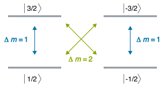
Figure 1: Scheme of the energy spectrum and the available transitions of a quadrupolar nucleus of spin 3/2. The transitions labeled with $\lvert\Delta m\rvert=1$ involve the exchange of a single photon, while those labeled $\lvert\Delta m\rvert=2$ involve two photons.

A first notable example is represented by the pure NQR of a spin 3/2 nuclei whose energy levels and available transitions are depicted in Figure 1. This system may undergo two single photon transitions at the same frequency, namely $\ket{1/2}\leftrightarrow\ket{3/2}$ and $\ket{-1/2}\leftrightarrow\ket{-3/2}$. This is in contrast with a pure NMR experiment where all the transitions are characterized by the same variation of the magnetic quantum number $\Delta m$. These two transitions imply an opposite change in the angular momentum of the system, so that each of them can occur only under the exchange of a photon with circular polarization (c.p.) $\sigma^{+}$ and $\sigma^{-}$, respectively. Therefore, when one irradiates the system by a linearly polarized (l.p.) resonant pulse, both transitions will be induced. In contrast, by choosing the proper polarization of the pulse one is able to select only one of the two. The potential of circularly and, in general, elliptically polarized RF pulses in NQR has been widely explored [64, 65, 66].

These theoretical expectations are correctly reproduced by our software. We simulated the pure NQR of a spin 3/2 ³⁵Cl nuclei in a potassium chlorate crystal (KClO₃), whose gyromagnetic ratio is $\gamma/2\pi=4.17$ MHz/T and whose quadrupolar resonance frequency is $\nu_{Q}=28.1$ MHz [67]. We prepared the system in the initial state depicted in Figure 2. Then, we performed two distinct simulations evolving the system under the action of a $\pi$ pulse with polarization $\sigma^{+}$ or $\sigma^{-}$ respectively (in a classical picture such pulses rotate the initial nuclear magnetization by 180^∘, clockwise and anticlockwise, respectively). The results obtained are shown in Figure 3. We note that the $\pi$ pulse is defined such that its amplitude, $B_{1}$, and time duration, $t_{P}$, satisfy the equation known as a central-transition selective pulse

$$\gamma\alpha B_{1}t_{P}=\pi$$ (19)

where $\alpha=\sqrt{I(I+1)-m(m+1)}$ is a factor depending on the transition being induced, and differs between the central and satellite peaks, and $\gamma$ is the gyromagnetic ratio of the nucleus. For the pulsing to be successful, the strength of the applied pulse $\gamma B_{1}$ must be smaller than the quadrupolar frequency $\omega_{Q}$. If the applied pulse is not perturbative relative to the quadrupolar energies, then the levels will mix instead of only rotating.

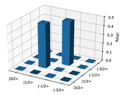
Figure 2: Real part of the density matrix representing the initial state of the spin 3/2 nucleus in the simulation of a pure NQR experiment. The system is prepared in a classical distribution where the states at the ground level are equally populated.

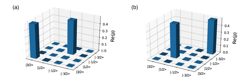
Figure 3: Real part of the simulated density matrix representing the evolved state of the spin 3/2 quadrupolar nucleus after: (a) a $\pi$ pulse with polarization $\sigma^{+}$; (b) a $\pi$ pulse with polarization $\sigma^{-}$.

The evolved density matrices clearly show that a pulse with circular polarization $\sigma^{+}$ ($\sigma^{-}$) couples only with the transition between states $\ket{1/2}\leftrightarrow\ket{3/2}$ ($\ket{-1/2}\leftrightarrow\ket{-3/2}$) by acting selectively on the two relevant energy eigenstates to induce a full inversion of their respective populations in such a way that the total angular momentum is conserved.

Another experiment where the pulse can be set up to selectively induce transitions is the NQR of a spin 1 nucleus in the presence of an asymmetric EFG [7]. Due to the non-vanishing asymmetry parameter, the energy eigenstates of this system are no longer the spin eigenstates, but they read:

$$\ket{0}\qquad\&\qquad\ket{\xi_{\pm}}=\left(\ket{1}\pm\ket{-1}\right)/\sqrt{2}$$ (20)

The energies of these states and the frequencies of transitions between them are displayed in Figure 4.

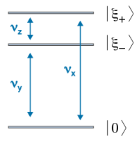
Figure 4: Scheme of the energy spectrum and the available transitions for a quadrupolar nucleus of spin 1 with an asymmetric EFG. The subscripts of the transition frequencies $\nu_{x/y/z}$ refer to the direction of linear polarization of the pulse required to induce each transition.

What is peculiar with this system is that in order for each of the three transitions to occur, the pulse must have a distinct linear polarization. Indeed, developing the calculations one finds that

$$I_{x}=\blockarray{cccc}\ket{\xi_{+}}&\ket{0}\ket{\xi_{-}}\\ \block{(ccc)c}010\ket{\xi_{+}}\\ 100\ket{0}\\ 000\ket{\xi_{-}}\\ \quad I_{y}=\left(\begin{array}[]{ccc}0&0&0\\ 0&0&1\\ 0&1&0\\ \end{array}\right)\quad I_{z}=\left(\begin{array}[]{ccc}0&0&1\\ 0&0&0\\ 1&0&0\\ \end{array}\right)$$ (21)

from which it is easy to prove that an $\mathbf{\hat{x}}$-, $\mathbf{\hat{y}}$- or $\mathbf{\hat{z}}$-polarized pulse will only affect the transition $\ket{\xi_{+}}\leftrightarrow\ket{0}$, $\ket{\xi_{-}}\leftrightarrow\ket{0}$, or $\ket{\xi_{+}}\leftrightarrow\ket{\xi_{-}}$, respectively. This behavior can be assessed by observing the spectrum generated by each of these pulses, recalling Eq. (18). Once the proper orientation of the detection coils is set, one is able to visualize if a certain transition has occurred depending on the whether the term $\matrixelement{\eta}{\rho(t_{P})}{\varepsilon}$ vanishes or not.

These results have been simulated in a fictitious spin 1 nucleus with $e^{2}qQ/h=1\,\rm{MHz}$ and asymmetry $\eta=0.6$, for which the transition frequencies are $\nu_{x}\equiv\nu_{\xi_{+}\leftrightarrow 0}=0.9\,\rm{MHz}$, $\nu_{y}\equiv\nu_{\xi_{-}\leftrightarrow 0}=0.6\,\rm{MHz}$, and $\nu_{z}\equiv\nu_{\xi_{+}\leftrightarrow\xi_{-}}=0.3\,\rm{MHz}$. The resulting NQR spectra are displayed in Figure 5.

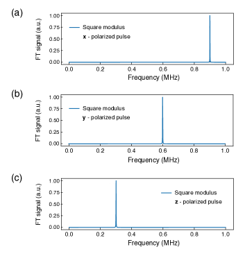
Figure 5: Spectra resulting from three distinct simulations of the NQR of a spin 1 nucleus in an asymmetric EFG, where different pulses have been applied with polarization along $\mathbf{\hat{x}}$ (a), $\mathbf{\hat{y}}$ (b), and $\mathbf{\hat{z}}$ (c), respectively.

4.2 Generation of quantum coherences in a spin 3/2 quadrupolar nucleus

Let us consider the spin 3/2 ³⁵Cl nucleus in the same KClO₃ crystal introduced above. In the previous example, we showed how to induce a full inversion of the populations of two of its energy eigenstates, say $\ket{m=1/2}$ and $\ket{m+1=3/2}$, by means of a $\sigma^{+}$ c.p. $\pi$ pulse of radiation. In general, when the angle on the right-hand side of Eq. (19) is set to a value different from $n\pi$, where $n$ is an integer, the final density matrix exhibits non-zero off-diagonal elements, meaning that the evolved state includes a quantum superposition of $\ket{m}$ and $\ket{m+1}$. Such superposition states can be deployed to probe nature of tensor multipolar orders [54, 32]. In NMR, such elements are typically called “single quantum coherences”, where “single” specifies the fact that $\Delta m=1$.

In Figure 6, we display the results of three simulated experiments where a pulse resonant with the $\ket{1/2}\leftrightarrow\ket{3/2}$ transition is applied and the angle in Eq. (19) is set to the values $\pi/3$, $\pi/2$, and $2\pi/3$, respectively. These simulations demonstrate that it is possible to fine-tune the amplitudes of two states linked by a single-photon transition through the careful manipulation of the parameters of the pulse.

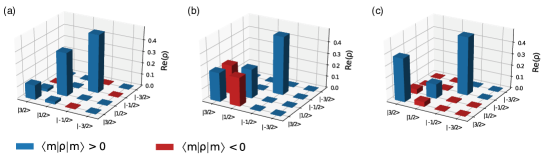
Figure 6: Results of the simulation of the NQR of ³⁵Cl nuclei in a KClO₃ crystal where a pulse resonant with the $\ket{1/2}\leftrightarrow\ket{3/2}$ transition is applied. The three histograms show the real part of the density matrix of the system evolved after (a) $\pi/3$ pulse, (b) $\pi/2$ pulse, and (c) $2\pi/3$ pulse. As the angle of rotation approaches $\pi$, the populations of the states involved in the transition undergo a continuous exchange, and at the same time non-zero, off-diagonal elements emerge between them, meaning that the two states are in a quantum superposition.

4.3 Preparation of an ensemble of spin 3/2 nuclei in a pseudopure state by means of NQR

NMR and NQR are naturally suited for the implementation of simple quantum information processors, as they are an efficient and high-precision method for manipulating nuclear spins [68, 69, 70, 18, 71]. Nonetheless, in typical NMR/NQR experiments the system under study is a macroscopic sample made up of a huge number of nuclei, which makes it impossible to prepare it in a pure state as would be required by an ordinary quantum computation protocol. This problem has been addressed by following a different strategy [9]: by means of a properly designed pulse sequence, the ensemble of nuclear spins can be prepared in a pseudopure state, i.e. a state $\rho=a\mathbbm{1}+b\outerproduct{\psi}{\psi}$ which differs from a pure state by a term proportional to the identity. A state of this kind is called pseudopure because, under evolution, it behaves like a full-fledged pure state. This property makes it the ideal starting point for any NMR/NQR quantum computation protocol. Indeed, much effort has been made in realizing quantum logic gates [72, 73, 74, 15, 2, 75, 76, 77, 78, 79, 80].

In what follows, we describe a simulation of the NQR protocol aimed at realizing a 2-qubit pseudopure state in the ensemble of spin 3/2 quadrupolar ³⁵Cl nuclei of a KClO₃ crystal [42], whose energy levels and available transitions have already been shown in Figure 1. The states of the 2-qubit computational basis correspond to the spin ones as follows:

$$\begin{array}[]{ccc}\ket{00}&\equiv&\ket{3/2}\\ \ket{01}&\equiv&\ket{1/2}\\ \ket{10}&\equiv&\ket{-1/2}\\ \ket{11}&\equiv&\ket{-3/2}.\\ \end{array}$$ (22)

Here, we remark that the simulated protocol is not aimed at implementing the pseudopure state in the physical system itself. Such a state is obtained as the average of the results of three distinct experiments, as depicted in Figure 7, following a common practice employed in NMR/NQR called temporal averaging [81]. In each of the three experiments, the system is handled in a distinct way:

1. In the first, the system is left in its original thermal equilibrium state.

2. In the second, the system is irradiated by a c.p. pulse with resonant frequency $\nu_{Q}=(E_{\pm 3/2}-E_{\pm 1/2})/h$, inducing one of the single photon transitions ($\lvert\Delta m=1\rvert$). The time duration of the pulse is set to a value such that the populations of the states linked by the transition are exchanged.

3. In the third, a c.p. pulse at half the resonance frequency is applied, yielding one of the two-photons transitions ($\lvert\Delta m=2\rvert$). Again, the time duration of the pulse accounts for the exchange of the populations of the states linked by the transition.

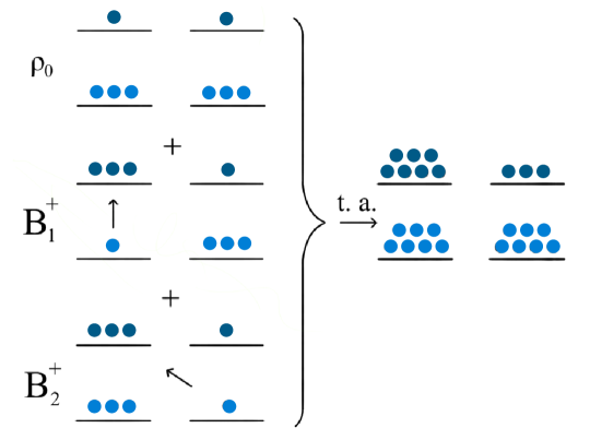
Figure 7: Population diagrams of the states to be combined through temporal averaging in order to realise the $\ket{11}=\ket{-3/2}$ pseudopure state in a spin 3/2 quadrupolar nucleus.

If the polarization of the pulses applied in steps 2 and 3 are appropriately chosen, the average of the density matrices resulting from the three experiments will have the properties of a pseudopure state belonging to the computational basis in Eq. (22). The outcomes of the simulation, illustrating the real part of the density matrices representing the four pseudopure states of the computational basis of 2 qubits, are shown in Figure 8.

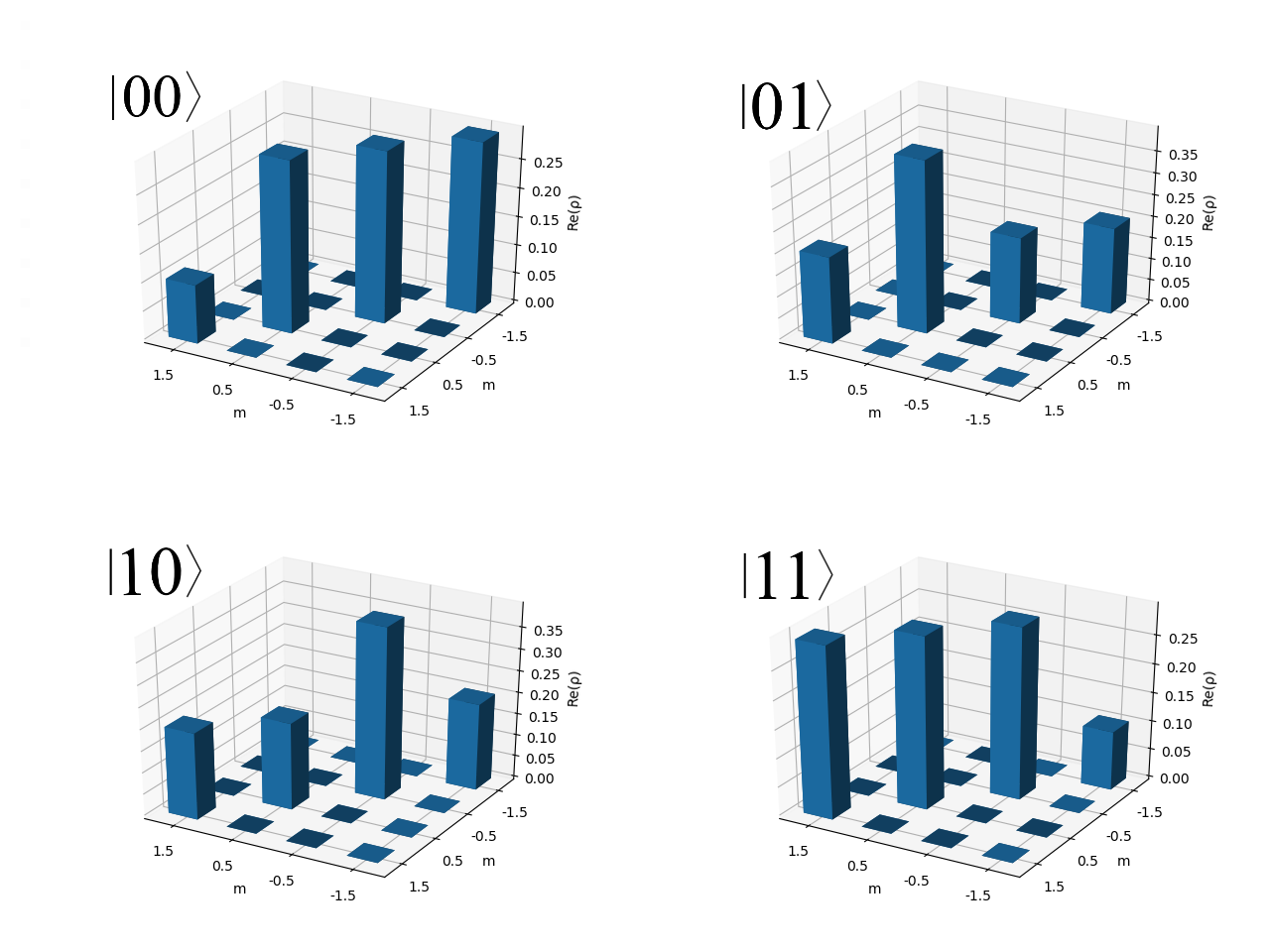
Figure 8: Outcomes of the protocol for the realization of pseudopure states in an ensemble of spin 3/2 quadrupolar nuclei, as simulated by our software. The histograms display the real part of the density matrices representing the four pseudopure states of the computational basis of 2 qubits.

4.4 NQR and NMR implementation of a CNOT gate on a couple of qubits

Implementing a CNOT gate in the system we have already discussed in subsection 4.3 is a straightforward task. That is, in a 2-qubit system with $\ket{0}$ and $\ket{1}$ as the only allowed input values for both qubits, the CNOT gate flips the second (target) qubit from $\ket{0}$ to $\ket{1}$ if and only if the first (control) qubit is in the $\ket{1}$ initial state. Indeed, one can easily check that the action performed by a CNOT₁ gate on the 2-qubit system is equivalent to that of a pulse which yields an exchange of the populations of the states $\ket{-1/2}$ and $\ket{-3/2}$, as illustrated in Figure 9a. The effect of this gate as simulated by our software and is depicted in Figure 9b.

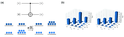
Figure 9: (a) Symbolic notation of a CNOT gate operating on the state $\ket{10}$ (on top) and the action of the pulse which carries out the equivalent operation on the NQR version of the 2-qubit system (at the bottom). (b) Input (on the left) and output (on the right) states of the simulated NQR CNOT₁ gate when the initial state is $\ket{10}$.

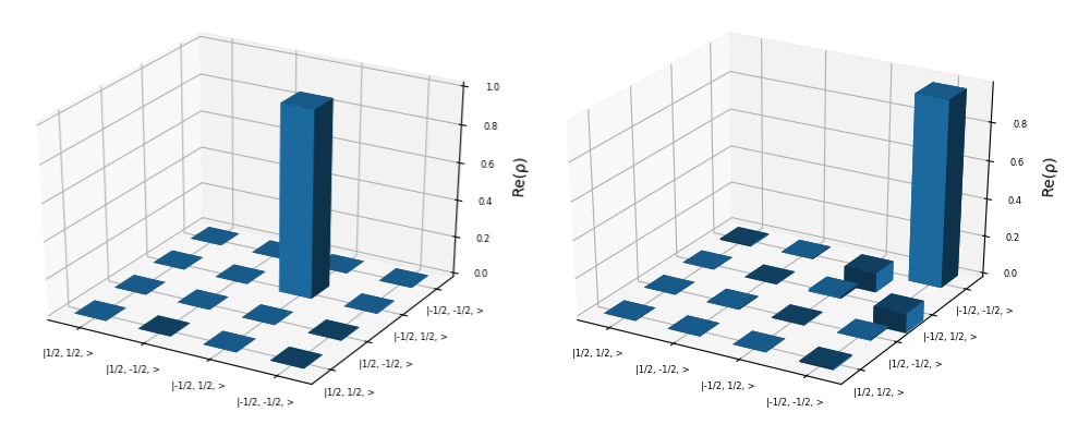
Figure 10: Input (on the left) and output (on the right) of the simulated NMR CNOT₁ gate when the initial state is set to the ideal pure state $\ket{10}$. The output state presents a slight discrepancy with respect to the expected $\ket{11}$ state, which is thought to be a consequence of the discrete approximations taken in the simulation.

It is possible to implement an analogous operation by means of NMR as well, but in a different nuclear system. As explained in [18], this time the 2 qubits are encoded in 2 distinct spin 1/2 nuclei (following the convention $\ket{0}\equiv\ket{1/2}$, $\ket{1}\equiv\ket{-1/2}$) and, in order for them to work as a control-target qubit couple, they must interact with each other. Thus, we assume that they are linked by the typical $J$-coupling, whose contribution to the Hamiltonian is:

$$\mathcal{H}_{J}=hJI_{z}^{(1)}I_{z}^{(2)}$$ (23)

where $J$ is the coupling constant and $I_{z}^{(i)}$ is the $z$ component of the spin of the $i$-th nucleus. The experimental protocol for the implementation of an NMR CNOT gate employs both selective rotations of each spin as well as the free evolution of the whole system under the action of $J$-coupling, according to the sequence:

$$\text{CNOT}_{1}=\left(-\frac{\pi}{2}\right)^{\mathbf{I}_{1}}_{z}\left(\frac{\pi}{2}\right)^{\mathbf{I}_{2}}_{z}\left(-\frac{\pi}{2}\right)^{\mathbf{I}_{2}}_{x}U\left(\frac{1}{2J}\right)\left(-\frac{\pi}{2}\right)^{\mathbf{I}_{2}}_{y}$$ (24)

Here, factors of the type $\left(\alpha\right)^{\mathbf{I}_{i}}_{x/y/z}$ represent pulses resonant with the $i$-th spin which make it rotate an angle $\alpha$ around the axis specified in the subscript. $U\left(1/2J\right)$, on the other hand, stands for the free evolution of the system for a time duration of $1/2J$. We point out that in order to be able to perform selective rotations of one of the two spins, the nuclei’s gyromagnetic ratios must be appreciably different, leading to well separated gyromagnetic frequencies $\nu_{0}^{(i)}=-(\gamma^{(i)}/2\pi)B_{0}$.

We have carried out a simulation of this protocol starting from ideal pure input states. The outcomes match closely our expectations, i.e. the initial ket is flipped since the control (second) qubit was in the $\ket{1}$ initial state, as is shown in Figure 10.

4.5 NMR probe of quantum correlations and tensor orders

As a local probe, NMR is well suited for the study of the microscopic electronic spin structure in the vicinity of the nuclear spin site through the hyperfine interaction. While directly measuring quantum correlations between electronic spins is difficult, complex hyperfine interactions can imprint signatures of electronic correlations on the nuclear spin states. The resulting many-body nuclear spin correlations can then be probed using the method of multiple quantum NMR [82, 83, 84]. The main challenge with this effort is that nuclear spin states are not pure states precluding the direct application of standard quantum protocols, which can be addressed by using pseudo-pure states (sec. 4.3). PULSEE can be instrumental in designing the optimal multiple quantum NMR sequence to permit the study of quantum correlations.

Many of the theoretically identified complex quantum phases of materials are characterized by tensor orders (e.g. ferro-octupolar order) [32, 33] that possess zero local susceptibility, and for that reason, are evasive to standard experimental probes. However, the tensor nature of the hyperfine interactions can reveal the intricate structure of quantum orders. In this section, we illustrate ways in which PULSEE is deployed to put forward a novel NMR method, inspired by QIS, that allows for the engineering of pulse sequences that can effectively probe electronic correlations and tensor orders through the hyperfine interaction.

In order to explore the capabilities of PULSEE, we give a simple yet powerful illustration of two approaches to modeling the hyperfine interaction. In the first, we considering a spin-1/2 nucleus coupled to an electronic bath directly via a hyperfine interaction ($\mathcal{H}_{\rm hf}=\mathbf{S}\tilde{A}\mathbf{I}$). In the second, we examine two spin-1/2 nuclei interacting via an effective hyperfine field, $\tilde{A}$, mediated via electrons ($\mathcal{H}_{\rm hf}=\mathbf{I_{1}}\tilde{A}\mathbf{I_{2}}$). The system will be modeled as two interacting spin-1/2 particles, governed by the Hamiltonian,

$$\mathcal{H}=-\omega_{n}(I^{(1)}_{z}\otimes\mathbbm{1})+\begin{cases}-\omega_{s}(\mathbbm{1}\otimes S_{z})+\mathbf{S}\tilde{A}\mathbf{I^{(1)}},&\text{i}\\ \\ -\omega_{n}(\mathbbm{1}\otimes I^{(2)}_{z})+\mathbf{I^{(1)}}\tilde{A}\mathbf{I^{(2)}},&\text{ii}\end{cases}$$ (25)

where $I,S$ correspond to the nuclear/electronic spin operator, respectively. The electronic Larmor precession frequency is much greater than the nuclear precession, $\omega_{s}\approx 2000\omega_{n}$, and the Zeeman terms dominate over the hyperfine coupling.

The two forms of the hyperfine interactions are written for different applications. For instance, the Hamiltonian defined in Eq. 25i may be useful in organic materials that exhibit very rich phase diagrams induced by strong correlations [85]. The concepts introduced in the study of open quantum systems [86] can be exploited to discern the nature of complex phases arising as a result of strong correlations. That is, a target system is identified as nuclear spins (e.g. ¹³C) coupled to the electronic bath via the hyperfine interaction, to an uncontrollable bath as correlated electron spins, and to an engineered auxiliary system as nuclear spins interacting via the dipole-dipole interactions. The target and auxiliary systems share an entangled state, reflecting the nature of the electronic correlations we seek to identify. By simulating the form of the expected experimental results, one may deploy PULSEE to devise effective pulse sequences to probe the quantum orders in such correlated phases. Furthermore, Eq. 25i can serve as a starting point for quantum control studies [87, 26, 88, 89, 85].

On the other hand, the Hamiltonian defined in Eq. 25ii may be useful in studies of mean-field electronic correlations and in the development of the probes of tensor order [90].

Here, we demonstrate the utility of PULSEE in devising an efficient protocol to probe the nature of tensor order, i.e. anisotropy of the hyperfine tensor. We consider two spin-1/2 spins coupled via a hyperfine interaction of the form,

$$\tilde{A}=\begin{pmatrix}A_{aa}&0&A_{ac}\\ 0&A_{aa}&0\\ A_{ac}&0&A_{aa}\end{pmatrix}$$ (26)

where $\tilde{A}$ is the second-rank hyperfine tensor representation for the antiferromagnetic phase (AFM) with symmetry plane $y=0$ [91]. The diagonal terms ($A_{aa}$) of $\tilde{A}$ dominate, giving the principal axes. The system will be modeled as two interacting spin-1/2 particles, governed by the Hamiltonian Eq. 25i. Working in the Zeeman-dominant regime, we investigate the evolution of the coherent spin state (CSS), as we have identified these as the most sensitive to anisotropy of the hyperfine tensor. Tuned to the nuclear spins, we can only probe the system by sending pulses to the nucleus. In the high-temperature limit, the thermal state of our system is given by

$$\rho_{\text{thermal state}}\approx\alpha\mathbbm{1}-\epsilon_{s}S_{z}-\epsilon_{n}I_{z},$$ (27)

where $\epsilon_{s}=\frac{\hslash\omega_{s}}{k_{B}T},\epsilon_{n}=\frac{\hslash\omega_{n}}{k_{B}T}\sim 10^{-6}\ll 1$ are the polarization factors at room temperature $T$, with two different deviation density matrices for the uncorrelated electronic and nuclear spins, $\alpha$ is a constant that depends on the temperature and Hamiltonian of the system, and where $\hslash/k_{B}$ is the Planck/Boltzmann constant. We work in units of $\hslash=1$. To obtain the CSS for the nucleus, one can transform the thermal state into a state of the form

$$\rho_{\text{CSS nucleus}}\approx\alpha\mathbbm{1}-\epsilon_{s}\mu-\epsilon_{n}\sigma,$$ (28)

where $\mu$ is the polarized state of the electron, given by $\mu=\ket{1}\bra{1}$, whenever the electrons are in a magnetically ordered state [91], and $\sigma$ is the deviation matrix of the nuclear spin’s CSS. The CSS saturates the Heisenberg uncertainty relation [92] and resembles a semiclassical spin. It is of the form

$$\ket{\zeta(\theta,\varphi)}=\sum_{m=-j}^{j}\binom{2j}{j+m}^{1/2}\cos^{j+m}\frac{\theta}{2}\sin^{j-m}\frac{\theta}{2}e^{i(j-m)\varphi}\ket{j,m},$$ (29)

where $j$ is the nuclear spin number, which in our case is $j=1/2$, $\theta,\varphi$ are angles in the Bloch sphere, and $\ket{j,m}$ are the eigenstates of the $I_{z}$ operator [92]. In principle, these angle give the rotation of the $I_{z}$ operator, and the CSS are eigenstates of the rotated $I_{z}$ operator, namely

$$(\vec{R}_{\theta\varphi}I_{z}\vec{R}_{\theta\varphi}^{\dagger})\ket{\zeta(\theta,\varphi)}=j\ket{\zeta(\theta,\varphi)},$$ (30)

for the rotation operator, $\vec{R}_{\theta\varphi}=e^{i\theta(I_{x}\sin\varphi-I_{y}\cos\varphi)}$. The angles $\theta=\pi/2$ and $\varphi=\pi/2$ are chosen for the particular case when there is no squeezing and the squeezing parameter is unity [93, 94]; thus the deviation matrix is $\sigma=\ket{\zeta(\pi/2,\pi/2)}\bra{\zeta(\pi/2,\pi/2)}$. These nuclear spin coherent pseudopure states (NSCS) have been experimentally prepared using the adapted strongly modulated pulse [94].

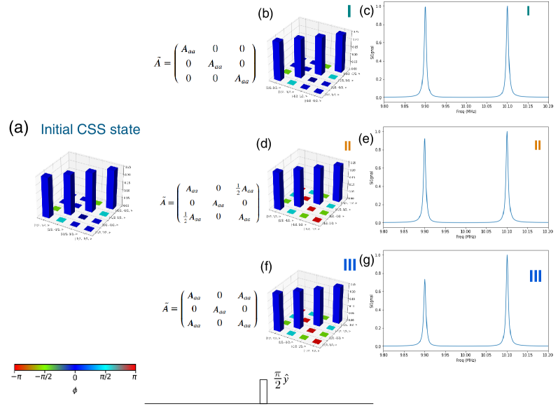
Figure 11: Dynamics of the (a) coherent spin state (CSS) (Eq. 28) in the high temperature limit. The system is evolved under the Hamiltonian (Eq. 25 i), a (b) $\pi/2$ pulse along $I_{x}$ is applied to the nuclear spin, (c) observing the corresponding NMR spectrum of the FID. Three simulations are given for the three different forms of the hyperfine tensor, I fully diagonal, II off-diagonal term $A_{ac}=\frac{1}{10}A_{aa}$, and III $A_{ac}=\frac{1}{5}A_{aa}$. This CSS is sensitive to the anisotropy of the hyperfine tensor, acting as an effective probe of tensor orders.

We perform a typical FID experiment simulation to obtain the NMR spectrum by evolving the initial state under the hyperfine Hamiltonian in Eq. 25i using the direct diagonalization method, applying a $\pi/2$ pulse to the nuclear spin, and observing the FID. We have assumed that $B_{0}=10\,\rm{T}$ and $T_{2}=50\,\mu\rm{s}$ and a 20 times longer acquisition time. The hyperfine coupling is much weaker than the Zeeman term (on the order of few percent of the nuclear Zeeman term) and it creates a peak splitting proportional to $A_{aa}$ (Fig. 11c & Fig. 12c).

We consider three different hyperfine tensors of the form depicted in Eq. 26, with $A_{ac}=0,A_{ac}=\frac{1}{2}A_{aa}$, and $A_{ac}=A_{aa}$. The form of the spectra and the evolved density matrices are given in Fig. 11. Using PULSEE, we have explored the sensitivity of various nuclear spin states to the form of the hyperfine tensor. We found that the particular CSS (Eq. 28) is sensitive to the anisotropy of the hyperfine tensor. That is, the relative height of one of the peaks in the splitting changes as a function of the strength of the off-diagonal term $A_{ac}$. What is promising about this method is the fairly straight forward way to implement it experimentally. Once the correct CSS is prepared for the nucleus, the system is perturbed by a simple $\pi/2$ pulse along the appropriate axis, in this case $I_{y}$. Our method is similar to the spin squeezing techniques in NMR pseudo-pure states [95].

Working only with a diagonal hyperfine tensor, we show that a CNOT gate implementation (Eq. 24) mimics the effects of the hypefine tensor (Fig. 12). In essence, the CNOT gate introduces entanglement, where the first nuclear site is the “control qubit” and the second nuclear site is the “target qubit.”

The combination of these two experiments gives us valuable information about the hyperfine tensor by studying the simple NMR spectrum. Firstly, we see that the central line of the Zeeman spectrum is split, where the splitting is given by the parameter $A_{aa}$ of the hyperfine tensor. Furthermore, the application of the CNOT gate (Eq. 24, where the last two $I_{z}$ pulses can be ignored, and $U=U(1/2A_{aa}$)) suppresses one of the peaks, Fig. 12f, as expected [76, 78]. Thorough investigation of the spin dynamics evolution after the application of the CNOT gate, allows us to establish the methodology for full hyperfine tensor determination.

Thus, measurements on CSS states serve as control experiments to sense the anisotropic nature of the hyperfine interaction. In other words, by performing rather manageable experiments, one may determine the nature of the hyperfine interaction, that is, the presence of off-diagonal terms, without the need of full field rotation spectroscopy [53]. Even though this simple experiment is only tuned to the nucleus, one may envision different ways to couple to the electronic spin [87, 22], and then use PULSEE to investigate the dynamics of the spin and the observables.

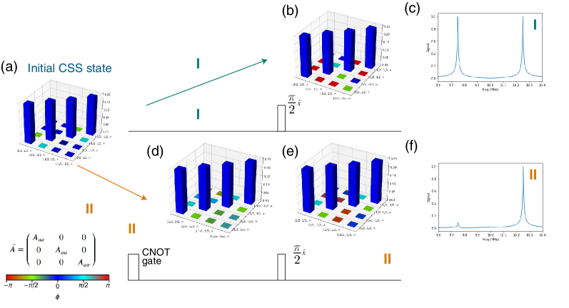
Figure 12: Dynamics of the (a) coherent spin state (CSS) (Eq. 28) in the high temperature limit. The system is evolved under the Hamiltonian (Eq. 25 i), and a (b) $\pi/2$ pulse along $I_{x}$ is applied to the nuclear spin, (c) observing the corresponding NMR spectrum of the FID. The bottom row is a second experiment (II), where a (d) CNOT gate (Eq. 24) is applied (e) before the $\pi/2$ pulse, (f) after which the FID is observed. This shows that the CNOT gate can mimic the effect of the anisotropic hyperfine tensor on the CSS.

In summary, our software allows for the simulation of complex spin evolution, which may then be used to design the appropriate pulse sequences enabling reverse engineering of the relevant Hamiltonians of tensor orders.

4.6 Building quantum circuits module: correlated density matrices

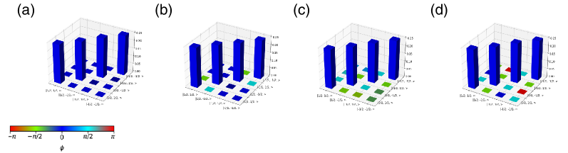
Figure 13: Effects of the pulse artifacts on the preparation of the nuclear spin coherent states (NSCS, Eq. 28) of a combined electronic-nuclear spin system, evolved under the second order average Hamiltonian theory mode. (a) Density matrix of initial thermal state (Eq. 27) is shown for comparison, where $\phi$ is the phase. (b) Theoretical NSCS generated by instantaneous perfect pulses from Eq. 29). NSCS prepared by applying a $\pi/2$ pulse along $I_{x}$, evolved under the (c) Zeeman and (d) both Zeeman and hyperfine Hamiltonians (Eq. 25 $A_{ac}=0$). By simulating finite NMR pulses, the evolved density matrix deviates from the theoretical one, even in the simple Zeeman case without any noise. Nevertheless, the gate fidelities (Eq. 31) of (c, d) are nearly unity.

The software supports designing quantum circuits via QubitState objects in the Quantum_computing module, and tracking the dynamics of a density matrix as it evolves in the circuit. Besides being useful for quantum circuit analysis, this module is instrumental in investigating the effects of experimental artifacts, such as pulse imperfections. The effects of finite pulses applied in the lab cannot be equated with the those of instantaneous perfect gates. The artifacts of ‘imperfect’ pulses need to be considered when performing complex NMR pulse sequences. In order to evaluate the errors associated with finite pulses, one may consider the gate fidelity defined by [96]

$$F=\frac{\Tr(\rho_{\text{th}}\cdot\rho_{\text{ex}})}{\Tr(\rho_{\text{th}}\cdot\rho_{\text{th}}^{\dagger})\Tr(\rho_{\text{ex}}\cdot\rho_{\text{ex}}^{\dagger})},$$ (31)

where $\rho_{\text{th}}$ is the theoretical density matrix, and $\rho_{\text{ex}}$ is the density matrix obtained experimentally through quantum tomography [97]. Using PULSEE, one may test finite pulses, determine the level of additional terms in the density matrix, and determine different pulse sequences and their fidelity in order to achieve the most adequate pulse train for the desired state evolution.

In Fig. 13 we illustrate the effect of the pulse artifacts on preparation of the nuclear spin coherent states (NSCS) using the average Hamiltonian theory method. The coherent spin state for a spin-1/2 particle whenever we use the angles $\theta=\pi/2$ and $\varphi=\pi/2$ is $\ket{\zeta(\pi/2,\pi/2)}=\ket{+y}$, or the ground eigenstate of the $I_{y}$ operator. In an NMR experiment, this $I_{y}$ state is obtained from a thermal state following the application a $\pi/2$ pulse along $I_{x}$. However, this assumes that the Hamiltonian which governs the system is a simple Zeeman one, and the $\pi/2$ pulse is perfect. We examine the effect of non-ideal $\pi/2$ pulse encountered when hyperfine interaction is present. Specifically, we simulate the effects of a non-ideal $\pi/2$ pulse by evolving the initial thermal state under two different Hamiltonians (Zeeman and hyperfine) and assume that no other noise in present in the system. Although the simulation does not include noise, we find that the density matrices differ when the full evolution of the pulse is considered under the different Hamiltonians, as depicted in Fig. 13. However, we learned that their fidelities do not notably differ from unity. These results demonstrate that in certain experiments one should examine the density matrices and not just consider fidelities to simulate proper time evolution of the spins.

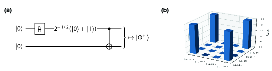
Figure 14: (a) Quantum circuit diagram of the application of a Hadamard and CNOT gate to produce a Bell state from the computational basis state $\ket{00}$. (b) Density matrix of correlated Bell state $\ket{\Phi_{+}}=2^{-1/2}(\ket{00}+\ket{11})$.

Theoretically predicted states can be modeled using the quantum computing module as a benchmark with experimentally prepared density matrices. As an example of the quantum circuit builder, consider constructing a two-qubit, “maximally-entangled” Bell state, produced by applying a Hadamard gate to one qubit, which creates a superposition, and then subsequently applying a CNOT-gate, which entangles the two qubits by creating a control and a target qubit. The gates’ matrix representations are

$$\hat{\text{H}}\equiv\frac{1}{\sqrt{2}}\begin{pmatrix}1&1\\ 1&-1\end{pmatrix}\quad\&\quad\text{CNOT}\equiv\begin{pmatrix}1&0&0&0\\ 0&1&0&0\\ 0&0&0&1\\ 0&0&1&0\end{pmatrix},$$ (32)

in the computational basis. Taking the initial state as $\ket{00}$, one obtains

$$\text{CNOT}[(\hat{\text{H}}\otimes\mathbbm{1})\ket{00}]=\text{CNOT}\left[\frac{1}{\sqrt{2}}(\ket{0}+\ket{1})\otimes\ket{0}]\right]=\frac{1}{\sqrt{2}}(\ket{00}+\ket{11}),$$ (33)

which is precisely the Bell basis state $\ket{\Phi^{+}}$. The circuit is depicted in Fig. 14(a), and the density matrix produced in Fig. 14(b).

Taking the control qubit as $A$, one may check that

$$\Tr(\rho_{\ket{\Phi^{+}}}^{A})=1/2<1,$$ (34)

confirming that this is indeed a correlated state [98].

5 Conclusions

PULSEE is an open-source software for the simulation of nuclear magnetic resonance experiments on complex materials. The main purpose of this program is to provide a numerical tool for the development of new methods of investigation of emergent properties in complex materials inspired by the NMR/NQR protocols established in the context of quantum information processing [99].

The software follows the principles of wide accessibility and intuitive utilization, being available for download from a public GitHub repository [51] and providing a GUI, Jupyter notebooks, as well as complete and detailed documentation.

The examples of execution illustrate the features of the software, which include the ability to simulate both the evolution of spin states and the corresponding experimental observables, and also highlight the possibilities to manipulate nuclear spin states through NMR/NQR. PULSEE enables simulations of the evolution of a single-spin under various interactions in solids. The investigation of the deviation of simulated results from experimental results on actual materials through the subsequent inclusion of different interaction terms in the Hamiltonian, opens up an opportunity to gain valuable insight into the microscopic nature of correlations in quantum materials. In that sense, our software might find its relevance in the design of highly sensitive protocols for the study of emergent quantum properties of materials.

6 CRediT author statement

Davide Candoli: Investigation, Software Programming, Development and Validation, Formal analysis, Visualization, Data curation, Writing-Original draft preparation. Ilija Nikolov: Software Programming, Development and Validation (NMR probe of Quantum correlations and quantum gates), Data curation, Writing-Original draft expansion. Lucas Z. Brito: Software Programming (Quantum.computing module), Development and Validation, Visualization, Testing. Stephen Carr: Software Programming, Development and Validation, Writing-Original draft expansion. Samuele Sanna: Methodology, Investigation, Supervision, Formal analysis, Resources, Reviewing and Editing. Vesna F. Mitrović: Conceptualization, Methodology, Supervision, Formal analysis, Visualization, Resources, Writing-Reviewing and Editing.

7 Acknowledgments

We thank Prof. Enrico Giampieri and Prof. Sekhar Ramanathan for their helpful advice during the development of the program. We are grateful to Jonathan Frassineti for the feedback as the very first user of the program. We also thank Prof. Paolo Santini and Prof. Alessandro Chiesa for reading the manuscript and providing helpful feedback. V. F. M. acknowledges support form the U.S. National Science Foundation grants OIA-1921199 and DMR-1905532.

Appendix A Form of Different Hamiltonians

The full Hamiltonian of a single-spin nuclear system is given in Eq. 1. Here we expand on terms that are less relevant for physics, but might be useful in other disciplines, along with their secular approximations in the Zeeman dominant regime. To start with, the hyperfine interaction given in Eq. 6 in the secular approximation becomes

$$\mathcal{H}_{HF}\approx AS_{z}I_{z}+BS_{z}I_{x},$$ (35)

for $A=a_{\text{iso}}+\hslash b_{D}(3\cos^{2}\theta-1),B=3\hslash b_{D}\sin\theta\cos\theta$, where $a_{\text{iso}}$ is the Fermi contact interaction constant. The chemical shift term, $\mathcal{H}_{CS}$, describes the local structure surrounding a nucleus, and thus it is very sample-specific. Its general form is given by

$$\mathcal{H}_{CS}=-\gamma\hslash\mathbf{I}\cdot\bm{\sigma}\cdot\mathbf{B}_{0},$$ (36)

where $\bm{\sigma}$ is the chemical shift tensor, given by

$$\bm{\sigma}=\begin{pmatrix}\sigma_{xx}&\sigma_{xy}&\sigma_{xz}\\ \sigma_{yx}&\sigma_{yy}&\sigma_{yz}\\ \sigma_{zx}&\sigma_{zy}&\sigma_{zz}\end{pmatrix}.$$ (37)

It depends on the overall electrons around the nuclear site, as well as the orientation of the sample with respect to $\mathbf{B}_{0}$. The chemical shift in the secular approximation is given by

$$\mathcal{H}_{CS}\approx-\gamma\hslash\sigma_{zz}(\Theta)B_{0},$$ (38)

where $\Theta$ is the angle between the molecule and the applied field. The dipolar Hamiltonian $\mathcal{H}_{D}$ is given by

$$\mathcal{H}_{D}=\hslash b_{D}\mathbf{I}^{T}_{1}\cdot D\cdot\mathbf{I}_{2},$$ (39)

where $b_{D}\equiv\frac{\mu_{0}\gamma_{1}\gamma_{2}\hslash}{4\pi r^{3}_{21}}$ is the dipolar constant, $\mu_{0}$ is the magnetic constant, $\gamma_{1},\gamma_{2}$ are the gyromagnetic ratio of two interacting spins, and $r_{21}$ is the average distance between the two spins. The quantity $D$ is the tensor that acts between the transpose of the spin operator of the first nucleus $\mathbf{I}^{T}_{1}$ and the spin operator of the second nucleus $\mathbf{I}_{2}$, and is given by

$$D=\begin{pmatrix}1-3\sin^{2}\theta\cos^{2}\varphi&3\sin^{2}\theta\sin\varphi\cos\varphi&3\sin\theta\cos\theta\cos\varphi\\ 3\sin^{2}\theta\sin\varphi\cos\varphi&1-3\sin^{2}\theta\sin^{2}\varphi&3\sin\theta\cos\theta\sin\varphi\\ 3\sin\theta\cos\theta\cos\varphi&3\sin\theta\cos\theta\sin\varphi&1-3\cos^{2}\theta\end{pmatrix},$$ (40)

where $\theta$ is the angle between the distance vector connecting the two spins and the external magnetic field $\mathbf{B}_{0}$, and $\varphi$ is the azimuthal angle. The dipolar coupling can be approximated in the Zeeman dominant regime for the homonuclear (nuclear-nuclear) & heteronuclear spins as

$$\mathcal{H}_{D1}\approx\hslash b_{D}\big{(}\frac{3\cos^{2}\theta-1}{2}\big{)}\big{[}3I_{1z}I_{2z}-\mathbf{I}_{1}\cdot\mathbf{I}_{2}\big{]},$$ (41)

and for the heteronuclear spin as

$$\mathcal{H}_{D2}\approx\hslash b_{D}\big{(}3\cos^{2}\theta-1\big{)}I_{1z}I_{2z}.$$ (42)

The J-coupling is given by

$$\mathcal{H}_{J}=2\pi\hslash\mathbf{I}_{1}\cdot\mathbf{J}\cdot\mathbf{I}_{2},$$ (43)

where $\mathbf{J}$ is the J-coupling tensor, given by

$$\mathbf{J}=\begin{pmatrix}J_{xx}&J_{xy}&J_{xz}\\ J_{yx}&J_{yy}&J_{yz}\\ J_{zx}&J_{zy}&J_{zz}\end{pmatrix}.$$ (44)

In the secular approximation, the J-coupling becomes

$$H_{J}\approx 2\pi\hslash JI_{1z}I_{2z},$$ (45)

where the $J$ constant is much smaller than the difference in the chemical shifts of the two sites [7].

References

- [1] F. A. Perras, C. M. Widdifield, and D. L. Bryce, “QUEST - Quadrupolar Exact Software: A fast graphical program for the exact simulation of NMR and NQR spectra for quadrupolar nuclei,” Solid State Nuclear Magnetic Resonance, vol. 45-46, pp. 36-44, (2012).
- [2] D. Possa, A. C. Gaudio, and J. C. C. Freitas, “Numerical simulation of NQR/NMR: Applications in quantum computing,” Journal of Magnetic Resonance, vol. 209, pp. 250-260, (2011).

References

-
[1]
L. M. K. Vandersypen, I. L. Chuang,
NMR techniques
for quantum control and computation, Rev. Mod. Phys. 76 (2005) 1037–1069.
doi:10.1103/RevModPhys.76.1037.
URL https://link.aps.org/doi/10.1103/RevModPhys.76.1037 -
[2]
C. Ramanathan, N. Boulant, Z. Chen, D. G. Cory, I. Chuang, M. Steffen,
Nmr quantum information
processing, Quantum Information Processing 3 (1) (2004) 15–44.
doi:10.1007/s11128-004-3668-x.
URL https://doi.org/10.1007/s11128-004-3668-x -
[3]
S. S. Hegde, J. Zhang, D. Suter,
Efficient
Quantum Gates for Individual Nuclear Spin Qubits by Indirect Control, Phys.
Rev. Lett. 124 (2020) 220501.
doi:10.1103/PhysRevLett.124.220501.
URL https://link.aps.org/doi/10.1103/PhysRevLett.124.220501 -
[4]
K. Modi, A. Brodutch, H. Cable, T. Paterek, V. Vedral,
The
classical-quantum boundary for correlations: Discord and related measures,
Rev. Mod. Phys. 84 (2012) 1655–1707.
doi:10.1103/RevModPhys.84.1655.
URL https://link.aps.org/doi/10.1103/RevModPhys.84.1655 -
[5]
E. N. Kaufmann, R. J. Vianden,
The electric field
gradient in noncubic metals, Rev. Mod. Phys. 51 (1979) 161–214.
doi:10.1103/RevModPhys.51.161.
URL https://link.aps.org/doi/10.1103/RevModPhys.51.161 -
[6]
W. P. Halperin,
Quantum size
effects in metal particles, Rev. Mod. Phys. 58 (1986) 533–606.
doi:10.1103/RevModPhys.58.533.
URL https://link.aps.org/doi/10.1103/RevModPhys.58.533 - [7] A. Abragam, Principles of Nuclear Magnetism, Oxford University Press, 1961.
- [8] R. Blinc, Magnetic resonance and relaxation in structurally incommensurate systems, Phys. Rep. 79 (1981) 331.
-
[9]
D. G. Cory, A. F. Fahmy, T. F. Havel,
Ensemble quantum
computing by NMR spectroscopy, Proceedings of the National Academy of
Sciences of the United States of America 94 (5) (1997) 1634–1639.
URL https://www.ncbi.nlm.nih.gov/pmc/articles/PMC19968/ - [10] I. L. Chuang, L. M. K. Vandersypen et al., Experimental realization of a quantum algorithm, Nature 393 (1998) 143–146. doi:https://doi.org/10.1038/30181.
-
[11]
J. A. Jones, M. Mosca, Implementation
of a quantum algorithm on a nuclear magnetic resonance quantum computer, The
Journal of Chemical Physics 109 (5) (1998) 1648–1653.
doi:10.1063/1.476739.
URL http://dx.doi.org/10.1063/1.476739 -
[12]
J. A. Jones, M. Mosca, R. H. Hansen,
Implementation of a quantum search
algorithm on a quantum computer, Nature 393 (6683) (1998) 344–346.
doi:10.1038/30687.
URL http://dx.doi.org/10.1038/30687 -
[13]
L. M. K. Vandersypen, M. Steffen, G. Breyta, C. S. Yannoni, R. Cleve, I. L.
Chuang, Experimental
realization of an order-finding algorithm with an nmr quantum computer,
Physical Review Letters 85 (25) (2000) 5452–5455.
doi:10.1103/physrevlett.85.5452.
URL http://dx.doi.org/10.1103/PhysRevLett.85.5452 -
[14]
G. Long, H. Yan, Y. Li, C. Tu, J. Tao, H. Chen, M. Liu, X. Zhang, J. Luo,
L. Xiao, X. Zeng,
Experimental
NMR realization of a generalized quantum search algorithm, Physics Letters
A 286 (2) (2001) 121–126.
doi:https://doi.org/10.1016/S0375-9601(01)00416-9.
URL https://www.sciencedirect.com/science/article/pii/S0375960101004169 -
[15]
N. Sinha, T. S. Mahesh, K. V. Ramanathan, A. Kumar,
Toward quantum
information processing by nuclear magnetic resonance: Pseudopure states and
logical operations using selective pulses on an oriented spin 3/2 nucleus,
The Journal of Chemical Physics 114 (10) (2001) 4415–4420.
arXiv:https://aip.scitation.org/doi/pdf/10.1063/1.1346645, doi:10.1063/1.1346645.
URL https://aip.scitation.org/doi/abs/10.1063/1.1346645 -
[16]
T. F. Havel, D. G. Cory, S. Lloyd, N. Boulant, E. M. Fortunato, M. A. Pravia,
G. Teklemariam, Y. S. Weinstein, A. Bhattacharyya, J. Hou,
Quantum information processing by
nuclear magnetic resonance spectroscopy, American Journal of Physics 70 (3)
(2002) 345–362.
arXiv:https://doi.org/10.1119/1.1446857, doi:10.1119/1.1446857.
URL https://doi.org/10.1119/1.1446857 -
[17]
T. Xin, B.-X. Wang, K.-R. Li, X.-Y. Kong, S.-J. Wei, T. Wang, D. Ruan, G.-L.
Long, Nuclear
magnetic resonance for quantum computing: Techniques and recent
achievements, Chinese Physics B 27 (2) (2018) 020308.
URL http://stacks.iop.org/1674-1056/27/i=2/a=020308 - [18] I. Oliveira, T. Bonagamba, R. Sarthour, J. Freitas, E. de Azevedo, NMR Quantum Information Processing, Elsevier, 2007.
-
[19]
K. R. K. Rao, T. S. Mahesh, A. Kumar,
Efficient
simulation of unitary operators by combining two numerical algorithms: An NMR
simulation of the mirror-inversion propagator of an spin chain, Phys.
Rev. A 90 (2014) 012306.
doi:10.1103/PhysRevA.90.012306.
URL https://link.aps.org/doi/10.1103/PhysRevA.90.012306 -
[20]
J. Teles, R. Auccaise, C. Rivera-Ascona, A. G. Araujo-Ferreira, J. P. Andreeta,
T. J. Bonagamba, Spin
coherent states phenomena probed by quantum state tomography in Zeeman
perturbed nuclear quadrupole resonance, Quantum Information Processing
17 (7) (2018) 177.
doi:10.1007/s11128-018-1947-1.
URL https://doi.org/10.1007/s11128-018-1947-1 -
[21]
D. Lu, K. Li, J. Li, H. Katiyar, A. J. Park, G. Feng, T. Xin, H. Li, G. Long,
A. Brodutch, J. Baugh, B. Zeng, R. Laflamme,
Enhancing quantum control
by bootstrapping a quantum processor of 12 qubits, npj Quantum Information
3 (1) (2017) 45.
doi:10.1038/s41534-017-0045-z.
URL https://doi.org/10.1038/s41534-017-0045-z -
[22]
Y.-X. Liu, A. Ajoy, P. Cappellaro,
Nanoscale
Vector dc Magnetometry via Ancilla-Assisted Frequency
Up-Conversion, Physical Review Letters 122 (10) (2019) 100501.
doi:10.1103/PhysRevLett.122.100501.
URL https://link.aps.org/doi/10.1103/PhysRevLett.122.100501 -
[23]
C. L. Degen, F. Reinhard, P. Cappellaro,
Quantum
sensing, Rev. Mod. Phys. 89 (2017) 035002.
doi:10.1103/RevModPhys.89.035002.
URL https://link.aps.org/doi/10.1103/RevModPhys.89.035002 -
[24]
P. Cappellaro, L. Jiang, J. S. Hodges, M. D. Lukin,
Coherence and
Control of Quantum Registers Based on Electronic Spin in a Nuclear Spin
Bath, Phys. Rev. Lett. 102 (2009) 210502.
doi:10.1103/PhysRevLett.102.210502.
URL https://link.aps.org/doi/10.1103/PhysRevLett.102.210502 -
[25]
F. Poggiali, P. Cappellaro, N. Fabbri,
Optimal control for
one-qubit quantum sensing, Phys. Rev. X 8 (2018) 021059.
doi:10.1103/PhysRevX.8.021059.
URL https://link.aps.org/doi/10.1103/PhysRevX.8.021059 -
[26]
H. Zhou, J. Choi, S. Choi, R. Landig, A. M. Douglas, J. Isoya, F. Jelezko,
S. Onoda, H. Sumiya, P. Cappellaro, H. S. Knowles, H. Park, M. D. Lukin,
Quantum Metrology
with Strongly Interacting Spin Systems, Phys. Rev. X 10 (2020) 031003.
doi:10.1103/PhysRevX.10.031003.
URL https://link.aps.org/doi/10.1103/PhysRevX.10.031003 -
[27]
P. Peng, C. Yin, X. Huang, C. Ramanathan, P. Cappellaro,
Floquet prethermalization
in dipolar spin chains, Nature Physics 17 (4) (2021) 444–447.
doi:10.1038/s41567-020-01120-z.
URL https://doi.org/10.1038/s41567-020-01120-z - [28] S. Carr, I. K. Nikolov, R. Cong, A. D. Maestro, C. Ramanathan, V. F. Mitrović, Multi-modal quantum spectroscopy of phase transitions with inversion symmetry, arXiv:2208.10987doi:10.48550/arXiv.2208.10987.
- [29] I. K. Nikolov, S. Carr, A. G. D. Maestro, C. Ramanathan, V. F. Mitrović, Spin squeezing as a probe of emergent quantum orders, under review at J. Phys. Soc. Jpn.
-
[30]
J. Johansson, P. Nation, F. Nori,
Qutip:
An open-source python framework for the dynamics of open quantum systems,
Computer Physics Communications 183 (8) (2012) 1760–1772.
doi:https://doi.org/10.1016/j.cpc.2012.02.021.
URL https://www.sciencedirect.com/science/article/pii/S0010465512000835 -
[31]
Quantum Machines, System software
company, Website.
URL https://www.quantum-machines.co -
[32]
L. V. Pourovskii, D. F. Mosca, C. Franchini,
Ferro-octupolar
order and low-energy excitations in double perovskites of
osmium, Phys. Rev. Lett. 127 (2021) 237201.
doi:10.1103/PhysRevLett.127.237201.
URL https://link.aps.org/doi/10.1103/PhysRevLett.127.237201 -
[33]
L. V. Pourovskii, S. Khmelevskyi,
Hidden order and
multipolar exchange striction in a correlated f-electron system, Proceedings
of the National Academy of Sciences 118 (14).
arXiv:https://www.pnas.org/content/118/14/e2025317118.full.pdf,
doi:10.1073/pnas.2025317118.
URL https://www.pnas.org/content/118/14/e2025317118 -
[34]
G. Wang, C. Li, P. Cappellaro,
Observation
of Symmetry-Protected Selection Rules in Periodically Driven Quantum
Systems, Phys. Rev. Lett. 127 (2021) 140604.
doi:10.1103/PhysRevLett.127.140604.
URL https://link.aps.org/doi/10.1103/PhysRevLett.127.140604 - [35] S. Carr, C. Snider, D. E. Feldman, C. Ramanathan, J. B. Marston, V. F. Mitrović, Signatures of electronic correlations and spin-susceptibility anisotropy in nuclear magnetic resonance, arXiv:2110.06811arXiv:2110.06811.
-
[36]
X. Turkeshi, T. Mendes-Santos, G. Giudici, M. Dalmonte,
Entanglement-Guided
Search for Parent Hamiltonians, Phys. Rev. Lett. 122 (2019) 150606.
doi:10.1103/PhysRevLett.122.150606.
URL https://link.aps.org/doi/10.1103/PhysRevLett.122.150606 -
[37]
W. Zhu, Z. Huang, Y.-C. He, X. Wen,
Entanglement
Hamiltonian of Many-Body Dynamics in Strongly Correlated Systems, Phys.
Rev. Lett. 124 (2020) 100605.
doi:10.1103/PhysRevLett.124.100605.
URL https://link.aps.org/doi/10.1103/PhysRevLett.124.100605 -
[38]
A. Allouche, G. Pouzard,
Computer
simulation of ft-nmr multiple pulse experiment, Computer Physics
Communications 54 (1) (1989) 171–176.
doi:https://doi.org/10.1016/0010-4655(89)90042-8.
URL https://www.sciencedirect.com/science/article/pii/0010465589900428 -
[39]
M. Bak, J. T. Rasmussen, N. C. Nielsen,
Simpson:
A general simulation program for solid-state nmr spectroscopy, Journal of
Magnetic Resonance 147 (2) (2000) 296–330.
doi:https://doi.org/10.1006/jmre.2000.2179.
URL https://www.sciencedirect.com/science/article/pii/S1090780700921797 -
[40]
K. Eichele,
Wsolids1
ver. 1.21.7.
URL http://anorganik.uni-tuebingen.de/klaus/soft/index.php?p=wsolids1/wsolids1 -
[41]
H. J. Reich,
Windnmr-pro,
Windows program (Feb. 2002).
URL https://www2.chem.wisc.edu/areas/reich/plt/windnmr.htm - [42] D. Possa, A. C. Gaudio, J. C. C. Freitas, Numerical simulation of NQR/NMR: Applications in quantum computing, Journal of Magnetic Resonance 209 (2) (2011) 250–260.
-
[43]
C. Bengs, M. H. Levitt,
Spindynamica:
Symbolic and numerical magnetic resonance in a mathematica environment,
Magnetic Resonance in Chemistry 56 (6) (2018) 374–414.
arXiv:https://analyticalsciencejournals.onlinelibrary.wiley.com/doi/pdf/10.1002/mrc.4642,
doi:https://doi.org/10.1002/mrc.4642.
URL https://analyticalsciencejournals.onlinelibrary.wiley.com/doi/abs/10.1002/mrc.4642 -
[44]
H. Hogben, M. Krzystyniak, G. Charnock, P. Hore, I. Kuprov,
Spinach
– a software library for simulation of spin dynamics in large spin systems,
Journal of Magnetic Resonance 208 (2) (2011) 179–194.
doi:https://doi.org/10.1016/j.jmr.2010.11.008.
URL https://www.sciencedirect.com/science/article/pii/S1090780710003575 -
[45]
M. Veshtort, R. G. Griffin,
Spinevolution:
A powerful tool for the simulation of solid and liquid state nmr
experiments, Journal of Magnetic Resonance 178 (2) (2006) 248–282.
doi:https://doi.org/10.1016/j.jmr.2005.07.018.
URL https://www.sciencedirect.com/science/article/pii/S1090780705002442 -
[46]
PERCH Solutions Ltd., Perch nmr
software.
URL http://new.perchsolutions.com/ -
[47]
F. A. Perras, C. M. Widdifield, D. L. Bryce,
QUEST
– Quadrupolar Exact Software: A fast graphical program for the exact
simulation of NMR and NQR spectra for quadrupolar nuclei, Solid State
Nuclear Magnetic Resonance 45-46 (2012) 36–44.
doi:https://doi.org/10.1016/j.ssnmr.2012.05.002.
URL https://www.sciencedirect.com/science/article/pii/S0926204012000586 -
[48]
Y. Binev, M. M. B. Marques, J. Aires-de Sousa,
Prediction of 1h nmr coupling
constants with associative neural networks trained for chemical shifts, J.
Chem. Inf. Model. 47 (6) (2007) 2089–2097.
doi:10.1021/ci700172n.
URL https://doi.org/10.1021/ci700172n -
[49]
T. Claridge, Software review of mnova:
Nmr data processing, analysis, and prediction software, J. Chem. Inf. Model.
49 (4) (2009) 1136–1137.
doi:10.1021/ci900090d.
URL https://doi.org/10.1021/ci900090d -
[50]
C. D. Schwieters, G. M. Clore,
The
vmd-xplor visualization package for nmr structure refinement, Journal of
Magnetic Resonance 149 (2) (2001) 239–244.
doi:10.1006/jmre.2001.2300.
URL https://www.sciencedirect.com/science/article/pii/S1090780701923006 -
[51]
D. Candoli, PULSEE (Program for
the simULation of nuclear Spin Ensemble Evolution (2021).
URL https://github.com/vemiBGH/PULSEE - [52] C. Snider, S. Carr, D. E. Feldman, C. Ramanathan, J. B. Marston, V. F. Mitrović, Simulation of spin echo and dynamics of interacting nuclear spins, To be submitted to Computer Physics Communications.
- [53] L. Lu, M. Song, W. Liu, A. P. Reyes, P. Kuhns, H. O. Lee, I. R. Fisher, V. F. Mitrović, Magnetism and local symmetry breaking in a Mott insulator with strong spin orbit interactions, Nature Communications 8 (14407).
-
[54]
R. Cong, R. Nanguneri, B. Rubenstein, V. F. Mitrović,
Evidence from
first-principles calculations for orbital ordering in
: A mott insulator with strong
spin-orbit coupling, Phys. Rev. B 100 (2019) 245141.
doi:10.1103/PhysRevB.100.245141.
URL https://link.aps.org/doi/10.1103/PhysRevB.100.245141 -
[55]
J. Zhang, S. S. Hegde, D. Suter,
Efficient
implementation of a quantum algorithm in a single nitrogen-vacancy center of
diamond, Phys. Rev. Lett. 125 (2020) 030501.
doi:10.1103/PhysRevLett.125.030501.
URL https://link.aps.org/doi/10.1103/PhysRevLett.125.030501 - [56] S. Blanes, F. Casas, J. A. Oteo, J. Ros, A pedagogical approach to the Magnus expansion, Eur. J. Phys. 31 (2010) 907–918.
- [57] C. P. Slichter, Principles of Magnetic Resonance, Springer-Verlag, 1990.
- [58] P. J. Hore, J. A. Jones, S. Wimperis, NMR: The Toolkit. How Pulse Sequences Work, Oxford, 2015.
-
[59]
M. A. McCoy, R. R. Ernst,