Discovery of a young pre-intermediate polar

Abstract

We present the discovery of a magnetic field on the white dwarf component in the detached post common envelope binary (PCEB) CC Cet. Magnetic white dwarfs in detached PCEBs are extremely rare, in contrast to the high incidence of magnetism in single white dwarfs and cataclysmic variables. We find Zeeman-split absorption lines in both ultraviolet Hubble Space Telescope (HST) spectra and archival optical spectra of CC Cet. Model fits to the lines return a mean magnetic field strength of $\langle|B|\rangle$ $\approx$ 600–700 kG. Differences in the best-fit magnetic field strength between two separate HST observations and the high $v\,\sin\,i$ of the lines indicate that the white dwarf is rotating with a period $\sim 0.5$ hours, and that the magnetic field is not axisymmetric about the spin axis. The magnetic field strength and rotation period are consistent with those observed among the intermediate polar class of cataclysmic variable, and we compute stellar evolution models that predict CC Cet will evolve into an intermediate polar in 7–17 Gyr. Among the small number of known PCEBs containing a confirmed magnetic white dwarf, CC Cet is the hottest (and thus youngest), with the weakest field strength, and cannot have formed via the recently proposed crystallisation/spin-up scenario. In addition to the magnetic field measurements, we update the atmospheric parameters of the CC Cet white dwarf via model spectra fits to the HST data and provide a refined orbital period and ephemeris from TESS photometry.

1 Introduction

Post Common Envelope Binaries (PCEBs) are systems containing at least one evolved star, in which the initial separation was close enough that the secondary was engulfed by the expanding envelope of the primary as it passed through the giant stages of its evolution. After double-degenerates, the second most common type of PCEBs are white dwarfs plus main-sequence companions (Toonen et al., 2017). The vast majority of the known systems of this kind contain a white dwarf and an M dwarf companion (Rebassa-Mansergas et al., 2010), although this is a selection effect as identification requires the white dwarf to be detectable against its main-sequence companion (Inight et al., 2021). For the remainder of this paper, we will use PCEB as synonymous for a close, detached binary consisting of a white dwarf and a main sequence companion that formed through a common envelope. The common envelope dramatically shrinks the binary separation, leaving most PCEBs with orbital periods of $\approx$ 0.1–5 d (Nebot Gómez-Morán et al., 2011). After emerging from the common envelope, PCEBs lose angular momentum via gravitational radiation (Paczynski & Sienkiewicz, 1981), and, if the main-sequence component possesses a convective envelope, magnetic wind braking (Rappaport et al., 1983). Consequently, the orbital separation decreases, eventually bringing the system into a semi-detached configuration, starting Roche-lobe overflow mass transfer from the companion onto the white dwarf – at this point, the PCEB will have evolved into a cataclysmic variable (CV).

Because these are stages along an evolutionary path, fundamental physical characteristics that are not expected to be affected by age or the mass transfer process should have the same distributions in both the PCEB and CV populations. This turns out not to be the case. Most prominently, the occurrence rate of white dwarfs with detectable magnetic fields is hugely discrepant between the two populations (Liebert et al., 2005).

In a volume-limited sample of 42 CVs, Pala et al. (2020) found that $36\pm 7$ per cent of the white dwarf primaries had magnetic field strengths $\gtrsim 1$ MG. Magnetic CVs are divided into polars with $B\gtrsim 10$ MG, where material from the secondary is accreted directly onto the poles of the white dwarf along the magnetic field lines, and intermediate polars with $0.1\la B\lesssim 10$ MG, in which an accretion disc is usually formed but truncated at the magnetospheric radius. Whereas the white dwarf spin periods of polars are locked to the binary period, the periods of intermediate polars are highly asynchronous, with some exhibiting spin periods of just a few tens of seconds (Patterson, 1979; Lopes de Oliveira et al., 2020).

The lack of an accretion disc around polars allows the white dwarf photosphere to be detected, enabling robust characterisation of the white dwarf parameters via spectral fitting and of the magnetic field strength and structure via detection of Zeeman-split lines and/or cyclotron emission (e.g. Schwope, 1990; Gänsicke et al., 2004; Ferrario et al., 1995). Conversely, very few robust measurements of the characteristics and magnetic field strengths of white dwarfs in intermediate polars exist, as the white dwarf is typically outshone by the accretion flow and the fields are too low to be detected via cyclotron emission from the accretion regions on the white dwarf. Variable polarised emission has been detected in a few intermediate polars (e.g. Potter & Buckley, 2018), providing loose constraints on their magnetic fields strengths consistent with the expected $B\lesssim 10$ MG range. Detecting and characterising “Pre-intermediate polars”, that is, white dwarfs with magnetic fields of $B\lesssim 10$ MG in detached binaries that have yet to be begin mass transfer, would therefore provide a useful insight into the unobservable properties of the intermediate polar population, such as the distributions of magnetic field strength and white dwarf mass.

However, in stark contrast to the CVs, magnetic white dwarfs in detached PCEBs are extremely rare. In a spectroscopic survey of over 1200 detached white dwarf plus M dwarf binaries, Silvestri et al. (2007) found just two candidate magnetic white dwarfs (which to our knowledge have not yet been confirmed or refuted), while Liebert et al. (2015) found no magnetic white dwarfs in a sample of 1735 binaries.

There are currently 16 PCEBs known with fields $>10$ MG (Reimers et al., 1999; Reimers & Hagen, 2000; Schmidt et al., 2005; Schmidt et al., 2007; Schwope et al., 2009; Parsons et al., 2021), which were identified via of the detection of either cyclotron or Balmer emission lines, spectral features that may have led to them being inadvertently excluded from the samples mentioned above. In the intermediate polar range, SDSS J030308.35+005444.1 ($B=8$ MG, Parsons et al., 2013) is the only unambiguous detection. These systems were initially thought to simply be polars with very low accretion rates (“LARPs”, e.g. Reimers et al., 1999), but it was soon realised that the companion stars were not quite filling their Roche lobes (e.g. Vogel et al., 2007) and the observed accretion was from stellar wind rather than mass transfer. They were therefore classified as pre-polars or PREPs, and we refer to them by that term henceforth. However, as discussed by Parsons et al. (2021) and Schreiber et al. (2021), it is likely that these systems were non-magnetic CVs in the past, which formed their magnetic fields via a combination of mass transfer induced spin up and crystallisation, entering a detached phase in the process. The secondaries are predicted to refill their Roche lobes in the future and thus the term pre-polar remains fitting, but these systems do not represent examples of the “missing” systems identified by Liebert et al. (2005); that is, magnetic white dwarfs in young PCEBs that have yet to undergo a period of mass transfer.

Here we present the first unambiguous detection of a magnetic white dwarf in a young PCEB. CC Cet (PG 0308+096) was identified as a post common envelope binary by Saffer et al. (1993) via radial velocity measurements of the H_α line, with a $\approx 6.9$ h orbital period confirmed by Somers et al. (1996). The system consists of a low-mass white dwarf ($\approx 0.4$ $\mathrm{M}_{\odot}$) with effective temperature ($T_{\mathrm{eff}}$) $\approx 25000$ K and an M4.5–5  dwarf secondary (Tappert et al., 2007) at a distance of $121.4\pm 1.1$ pc (Gaia Collaboration et al., 2018). We have obtained ultraviolet spectroscopy of the white dwarf component, revealing Zeeman-split absorption lines induced by a 600–700 kG magnetic field, indicating that CC Cet is a young, low-mass pre-intermediate polar.

The paper is arranged as follows: Section 2 describes the observations of CC Cet; Section 3 presents our model fitting process to the spectra to measure the white dwarf atmospheric parameters and magnetic field characteristics; in Section 4 we model the evolution of CC Cet and discuss the implications of our results for the study of magnetic white dwarfs in binaries. We conclude in Section 5.

2 Observations

Details of our spectroscopic observations of CC Cet are collated in Table 3.

2.1 Hubble Space Telescope

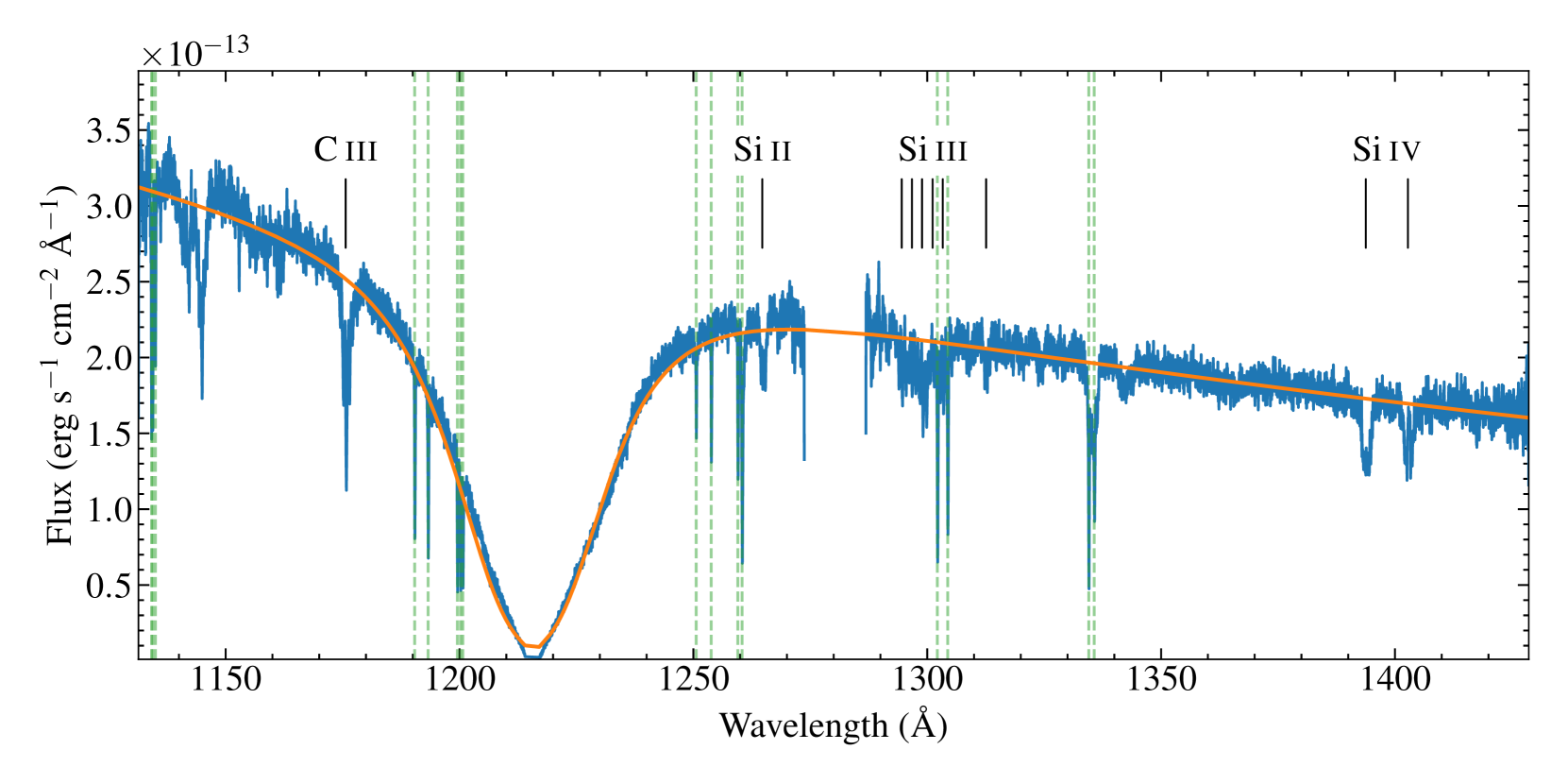
Figure 1: Full COS G130M spectrum of CC Cet obtained on 2018 February 01. The spectrum has been smoothed by a 5-point boxcar, matching the approximate oversampling rate of the COS detector. The best-fit model atmosphere spectrum is overplotted in orange. Rest wavelengths of the C and Si absorption lines discussed in the text are labeled, and interstellar absorption lines are marked with green dashed lines.

CC Cet was observed with the Cosmic Origins Spectrograph (COS, Green et al., 2012) onboard the Hubble Space Telescope (HST) as part of program ID 15189 (PI Wilson). Observations were obtained on 2018 February 1 and 2018 July 22 with exposure times of 1865 s each, using the G130M grating with a central wavelength of 1291 Å. The spectral resolution of this setup is $\approx 0.1$ Å per resolution element, or $\approx 20$ km s^-1. We abbreviate the two visits as the 2018 Feb and 2018 Jul spectra respectively throughout. The spectra were reduced using the standard calcos tools. Figure 1 shows the 2018 Feb spectrum with the absorption lines discussed below marked. Due to the combination of the radial velocity shifts induced by the binary orbit (see Section 3.3.9) and the magnetic splitting discussed below, we did not attempt to coadd the two spectra, instead analysing each one separately.

Of the other targets observed in program 15189, we use LM Com as a comparison example of a non-magnetic white dwarf with a similar $T_{\mathrm{eff}}$ and surface gravity ($\log g$) to CC Cet in several plots below. LM Com was observed on 2017 December 17 with an exposure time of 1815 s and otherwise the same details as the CC Cet observations.

2.2 TESS

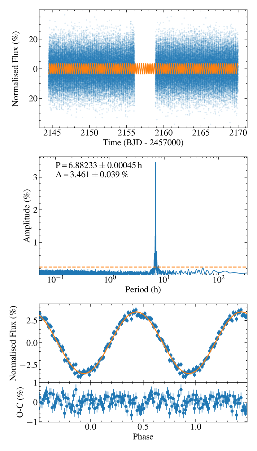
Figure 2: Top panel: TESS photometry of CC Cet with 20 s cadence (blue), with a model fit in orange. Middle panel: Lomb-Scargle periodogram of the TESS light curve, clearly showing the binary orbital period but with no evidence for any other periodicities. The orange dashed line shows the 0.01% false alarm probability. Bottom panel: Phase-folded light curve (blue) and sine model fit (orange), repeated for clarity. The residuals are shown as an O-C calculation.

CC Cet was observed by the Transiting Exoplanet Survey Satellite (TESS, TIC 337219837) in Sector 4 (2018 October 19–2018 November 14) at 30 min cadence and again in Sector 31 (2020 October 12–2020 November 22), for which both 2 min and 20 s cadence data was returned (GO 3124, PI Hermes). Figure 2 shows the results of our analysis of the 20 s data using Lightkurve (Lightkurve Collaboration, 2018). The false alarm probability was calculated following the recipe from Bell et al. (2019). The light curve shows clear sinusoidal variation with a period of $6.88233\pm 0.00045$ h, in agreement with the orbital period of the binary system measured by Somers et al. (1996). The photometric modulation has a constant amplitude, confirming that it is produced by irradiation of the M dwarf, which varies on the orbital period, rather than ellipsoidal modulation, which would induce an asymmetric double-peaked light curve. We calculated an updated ephemeris of TJD $=2459157.14634\pm 0.00052$, defined as the time of inferior conjunction nearest to the mid-point of Sector 31.

The results from the 20 s data were double-checked against a 30 min cadence light curve extracted from the Sector 4 data using the eleanor package (Feinstein et al., 2019), with no evidence found for significant changes in either the period or the amplitude of the modulation. Inspecting the power spectrum of the 20 s light curve, we find no evidence for additional periods between 40 s and $\approx 14$ d, adopting the 0.01 per cent False Alarm Probability of 0.25 per cent amplitude as an upper limit. We therefore detect no evidence for flux modulations induced by the white dwarf rotation (see Section 3.3.9) or any evidence that the M dwarf rotation is not tidally locked to the orbital period. Splitting the light curve into 0.5 d chunks, we found that the amplitude remained stable to within 1 $\sigma$ over the sector, and hence we do not detect evidence for modulation due to spots on the secondary star and/or differential rotation, as seen in V471 Tauri by Kővári et al. (2021). A visual inspection of the 20 s light curve found no significant flare events.

2.3 XMM-Newton

We obtained X-ray observations of CC Cet with the XMM-Newton (XMM) space telescope timed to overlap the two HST/COS visits: on 2018 February 1 at 23:05:40 UTC for a nominal exposure time of 5127s; and on 2018 July 22 at 03:56:09 UTC for a nominal exposure time of 15423s. The EPIC pn data were obtained in Large Window mode using the thin filter, with MOS1 and MOS2 employing Partial Window mode and the Medium filter. Data were processed using standard extraction methods within the XMM Science Analysis System version 18.0.0 to extract images, light curves, and spectra.

Unfortunately, both observations were severely afflicted with background flares, the first to such an extent that only a few hundred seconds of exposure were useful. By-eye inspection of those data revealed no obvious signs of a strong source, and so in the following we ignore the scant remaining 2018 February data. For the second observation, 6011s and 7828s of useful exposure time were retrieved for pn and MOS detectors, respectively. The pn image in the vicinity of the source position is illustrated in Figure 3.

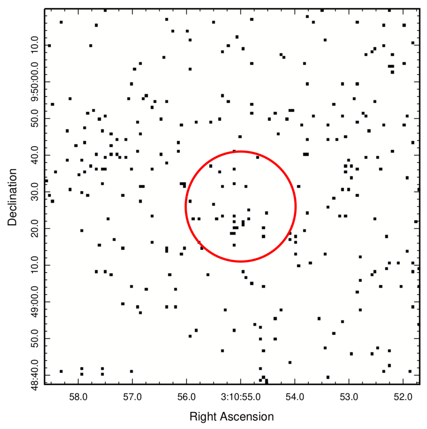
Figure 3: The XMM-Newton image in the pn detector of the vicinity around CC Cet. The red circle is centered on the position of CC Cet and has a radius of 15 arcsec. The 2x binned pixel scale is approximately 0.8 arcsec. The source is only detected at $<3\sigma$ significance, providing an upper limit on the X-ray flux.

The MOS1 and MOS2 data were combined prior to analysis. Source counts were extracted from both pn and MOS data using a circular region with a radius of 15 arcsec enclosing approximately $70\pm 5$% of the energy. This size of region was chosen because the XMM point spread function has very extended wings and enlarging the extraction region to encircle a greater fraction of the energy comes at the expense of significantly increasing the background. An annular region of area greater than ten times the source region and centered on the source position was used for estimating the background rate. The resulting count rates are listed in Table 1. While the source appears at a level greater than the background in both pn and MOS, neither represents a significant detection at greater than the $3\sigma$ level.

Table 1: Summary of XMM-Newton results

Parameter	pn	MOS
Net exposure (s)	6011	7828
$15\arcsec$ radius count rate (count ks-1)	$4.99\pm 0.91$	$3.45\pm 0.66$
Scaled background (count ks-1)	$3.17\pm 0.18$	$1.87\pm 0.13$
Net Source rate (count ks-1)	$1.82\pm 0.93$	$1.58\pm 0.66$
$L_{X}$ at $10^{7}$ K $(10^{27}$ erg s-1)a	$6.1\pm 2.3$	$10.8\pm 4.6$

^aX-ray luminosity assuming an optically-thin plasma radiative loss model with solar metallicity and an interstellar absorbing column of $2\times 10^{20}$ cm^-2 (see text).

2.4 VLT/UVES

CC Cet was observed with the Ultraviolet and Visual Echelle Spectrograph (UVES, Dekker et al., 2000) on the Very Large Telscope (VLT) as part of the Supernovae Type Ia Progenitor Survey (SPY, Napiwotzki et al., 2020; Koester et al., 2009). Two spectra were obtained on 2001 February 7–8, each covering the wavelength range 3281–6686 Å with $R\approx 21\,000$. We retrieved both spectra as fully calibrated data products from the ESO Archive Science Portal.

3 Modelling

3.1 White dwarf characteristics

Figure 1 shows the 2018 Feb COS G130M spectrum of CC Cet. The spectrum is typical of white dwarfs in this temperature range (Koester et al., 2014): dominated by the broad H i 1215.67 Å Lyman $\alpha$ line, along with a mixture of narrow and deep interstellar lines and broader, shallower photospheric lines. We detect no contribution from emission lines produced by the M dwarf, which is unsurprising given that the lack of flares in the TESS light curve indicates that the M dwarf is relatively inactive. The spectrum shows photospheric absorption lines of Si iv, implying that the $T_{\mathrm{eff}}$ of the white dwarf is higher than 25 000 K.

To estimate the atmospheric parameters of the white dwarf in CC Cet, i.e. $T_{\mathrm{eff}}$ and $\log g$, we fitted the continuum of the COS spectroscopy with a grid of synthetic white dwarf models computed with an updated version of the code described in Koester (2010), using the Markov Chain Monte Carlo (MCMC) technique. The Eddington flux ($f_{\text{Edd}}$) of the models were scaled as

$$F_{\rm obs}=4\,\pi\,\left(\mbox{$R_{\mathrm{wd}}$}\times\Pi\right)^{2}\,\times\,f_{\rm Edd}(\mbox{$T_{\mathrm{eff}}$},\mbox{$\log g$}),$$ (1)

where $\Pi$ is the parallax and $R_{\mathrm{wd}}$ is the white dwarf radius. $R_{\mathrm{wd}}$ is a function of $\log g$ and $T_{\mathrm{eff}}$ via the white dwarf mass-radius relation. We used the mass-radius relation for white dwarfs with hydrogen-rich atmospheres by interpolating the cooling models from Fontaine et al. (2001) with thick hydrogen layers of $M_{\rm H}/\mbox{$M_{\mathrm{wd}}$}=10^{-4}$, which are available from the University of Montreal website In addition the models were corrected by reddening ($E(B-V)$) using the extinction parameterization from Fitzpatrick (1999). In summary, the parameters to be fitted are: $T_{\mathrm{eff}}$, $\log g$, $\Pi$, and $E(B-V)$.

We set a flat prior on $\Pi$ using the Gaia DR2, parallax for CC Cet ($\Pi=8.2381\pm 0.0758$ mas, Gaia source id = 15207693216816512 Gaia Collaboration et al., 2018), which corresponds to a distance of $D=121.4\pm 1.1$ pc, and forced the fits to find the best parallax value within $1\sigma$. We set a Gaussian prior on the reddening of $E(B-V)=0.012\pm 0.015$ mag based on the measurement from the STructuring by Inversion the Local Interstellar Medium (stilism) at a distance of 120 pc. $T_{\mathrm{eff}}$ and $\log g$ were constrained to the values covered by our grid of model spectra.

The models have a pure hydrogen atmosphere with the parameter for mixing length convection set to 0.8. The grid spans $\mbox{$T_{\mathrm{eff}}$}=10\,000-35\,000$ K in steps of 200 K, and $\mbox{$\log g$}=7.0-9.0$ dex in steps of 0.1 dex.

Earth airglow emission lines from Lyman $\alpha$ and metal absorption lines from the interstellar medium (Table 4) and the white dwarf photosphere (C iii, Si ii, Si iii,Si iv, see below), were masked out during the process (see Figure 1).

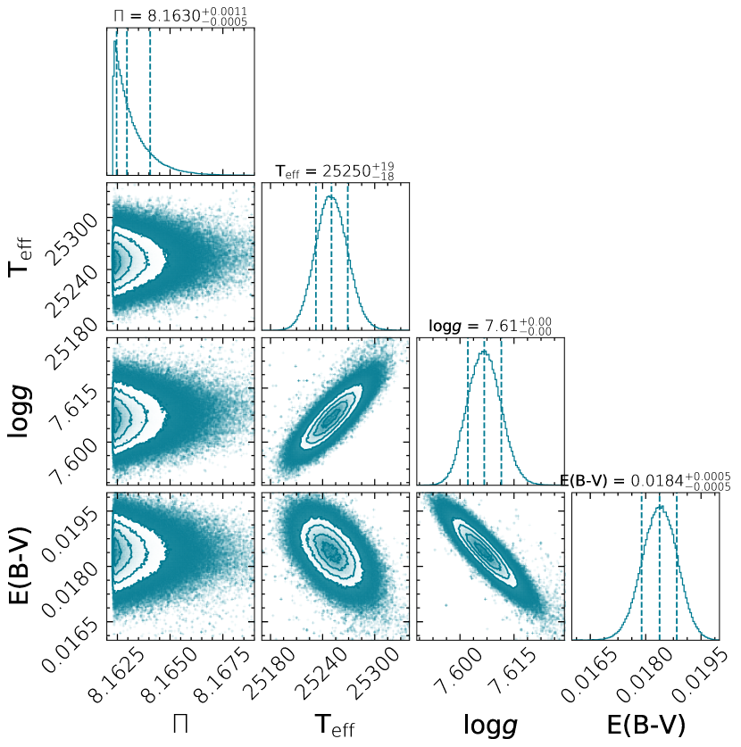
Figure 13: Results of the MCMC fit to the white dwarf atmospheric parameters plotted with corner.py (Foreman-Mackey, 2016).

We used the python-based emcee MCMC method (Foreman-Mackey et al., 2013), where 100 walkers were sampling the parameter space during 10 000 iterations. The likelihood function was defined as -0.5$\chi^{2}$. In general the walkers converged quickly, therefore we removed the first 250 steps from the chain. The full results are shown in Figure 13. The samples of $T_{\mathrm{eff}}$, $\log g$, and $E(B-V)$ follow a normal distribution, except the samples of the parallax which clustered towards the lower tail of the distribution. While the parallax was tightly constrained during the fits to be within $\pm 1\sigma$ from the Gaia average value, the results hint that larger distances are required to improve the far-ultraviolet spectroscopic fits of CC Cet. For the normal distribution, we considered the median as the best value and the 15.9^th and 84.1^th percentiles for one standard deviation as error. The intrinsic uncertainties from the MCMC method are very small and are purely statistical. The results are $\mbox{$T_{\mathrm{eff}}$}=25\,245^{+18}_{-19}$ K, $\mbox{$\log g$}=7.606^{+0.005}_{-0.004}$ dex, $E(B-V)=0.0183\pm 0.0005$ mag for the 2018 Feb COS spectrum and $\mbox{$T_{\mathrm{eff}}$}=25\,162^{+19}_{-20}$ K, $\mbox{$\log g$}=7.564\pm 0.005$ dex, and $E(B-V)=0.023\pm 0.0005$ mag for the 2018 Jul spectrum. We computed the mean and standard deviation using the two estimates of the parameters from the fits which account for systematic errors. These best-fit values are quoted in Table 2. We generated distributions for the mass and radius by drawing 10 000 pairs from normal distributions of $\mbox{$T_{\mathrm{eff}}$}=25\,203\pm 42$ K and $\mbox{$\log g$}=7.58\pm 0.02$ dex, then computing the mass and radius for each pair. We find two normal distributions for the mass and radius described by $\mbox{$M_{\mathrm{wd}}$}=0.441\pm 0.008$ $\mathrm{M}_{\odot}$ and $\mbox{$R_{\mathrm{wd}}$}=0.0179\pm 0.0003$ $\mathrm{R}_{\odot}$.

Table 2: Characteristics of the CC Cet system. References: 1. This work; 2. Gaia Collaboration et al. (2018); 3. Saffer et al. (1993); 4. Tappert et al. (2007); 5. Somers et al. (1996).

Parameter	Value	Reference
$T_{\mathrm{eff}}$ (K)	$25\,203\pm 42$	1
$\log g$ (cm s-2)	$7.58\pm 0.02$	1
$E(B-V)$ (mag)	$0.021\pm 0.002$	1
White dwarf Mass ($\mathrm{M}_{\odot}$)	$0.441\pm 0.008$	1
White dwarf Radius ($\mathrm{R}_{\odot}$)	$0.0179\pm 0.0003$	1
Parallax (mas)	$8.2381\pm 0.0758$	2
Distance (pc)	$121.4\pm 1.1$	1
Magnetic field strength (kG)	600–700	1
$v\sin i$ (km s-1)	$40\pm 10$	1
Secondary Mass ($\mathrm{M}_{\odot}$)	$0.18\pm 0.05$	3
Secondary Spectral Type	M4.5–5	3, 4
Orbital period (TESS, h)	$6.88233\pm 0.00045$	1
Ephemeris (TESS, TJD)	$2\,459\,157.14634\pm 0.00052$	1
Binary inclination (∘)	$35\pm 5.5$	5

3.2 Spectral lines in the COS spectra of CC Cet

The COS spectra of CC Cet contain multiple absorption lines of both interstellar and photospheric origin. The interstellar lines are invariably due to resonance lines of neutral or singly-ionised abundant elements such as C ii, N i, O i, Si ii, and S ii. Because the observed interstellar lines arise only from the lowest ground state level, it can sometimes happen that in a multiplet of resonance lines which is also present in the photospheric spectrum, only some of the lines of the multiplet are contaminated by interstellar scattering. This allows the photospheric lines to be reliably modelled without contamination from the interstellar lines.

The strongest photospheric lines present in the COS spectrum of CC Cet are primarily due to C iii (six lines at 1175 Å), Si iii (six lines between 1294 and 1303 Å), and Si iv (two lines at 1393 and 1402 Å). There are also two blended photospheric lines of Si ii at 1265 Å.

3.3 Magnetic field

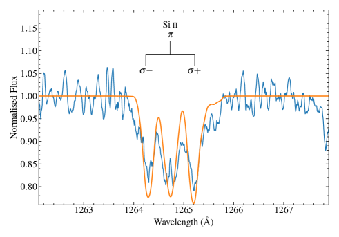
Figure 4: The Si ii 1264.738 Å line in the 2018 Feb spectrum (blue) compared with a model fit (orange). The line is Zeeman-split into a central $\pi$ and outer $\sigma$ components.

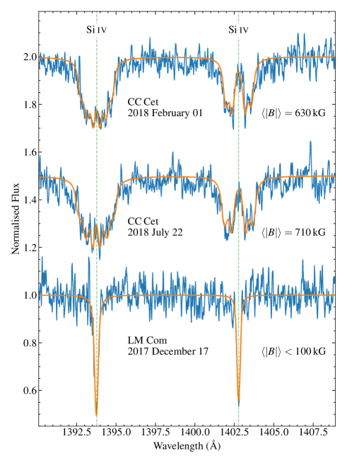
Figure 5: Silicon Si iv lines in the two HST/COS spectra of CC Cet, and one spectrum of LM Com, another PCEB with a similar $T_{\mathrm{eff}}$ and $\log g$. The difference between the Zeeman split lines in CC Cet and the non-magnetic LM Com is readily apparent. The orange line shows the best-fit magnetic model to the lines (in the case of LM Com corresponding to an upper limit on the field strength), and the dashed vertical lines show the rest wavelengths. The date and best-fit mean field modulus are given under each spectrum.

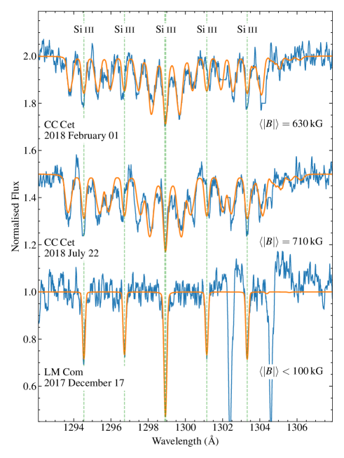
Figure 6: As Figure 5 but for Si iii lines around 1300 Å. The deep unmarked absorption features in the LM Com spectrum are interstellar O i lines that have been removed from the spectrum of CC Cet. Each line in LM Com is replaced in the spectrum of CC Cet by a Zeeman triplet. Note the slight mis-match between the centroids of some of the lines in the model and the spectrum induced by the partial Paschen-Back effect.

3.3.1 Discovery of field

Closer examination of the photospheric lines reveals that they differ significantly from those in similar COS spectra. In particular, the Si ii 1264 Å resonance line (which is slightly blended with a much weaker line in the same multiplet, but not blended with any interstellar lines because it arises from a state a few hundred cm^-1 above the ground level) shows a clear triplet structure composed of three very similar components separated by about 0.5 Å (Figure 4). The structure is strongly reminiscent of the appearance of the normal Zeeman triplet produced in many spectral lines by a magnetic field of tens or hundreds of kiloGauss (kG). The appearance of this feature strongly suggests that CC Cet has a magnetic field.

Furthermore, although the other strong photospheric lines do not show such obvious Zeeman splitting, they all look rather peculiar. The two Si iv lines around 1400 Å, which normally show very similar Lorentzian profiles, instead are quite broad and different from one another (Figure 5). The six strong lines of Si iii around 1300 Å appear as about 15 slightly weaker lines in the same wavelength interval (Figure 6). The C iii lines at 1175 Å show only three strong lines instead of the usual five (Figure 7). As we shall show below, these effects can be produced by a magnetic field of hundreds of kG.

3.3.2 Qualitative analysis of field

To obtain further information about the magnetic field which appears to be present in CC Cet, we start by estimating the mean field modulus $\langle|B|\rangle$, the value of the local field strength $|{\bf B}|$ averaged over the hemisphere visible at the time of observation. The observed splitting of the Si ii 1264 Å  line is about 0.5 Å between each of the $\sigma$ components and the central $\pi$ component. This value may be used with the standard equation for the $\pi$ – $\sigma$ separation $\Delta\lambda_{\rm Z}$ due to the normal Zeeman effect for an initial field strength estimate (e.g. Landstreet, 1992):

$$\Delta\lambda_{\mathrm{Z}}(\mbox{\AA})=4.67\times 10^{-13}z\lambda_{0}^{2}B,$$ (2)

where $\lambda_{0}$ is the unperturbed wavelength of the line, wavelengths are measured in Å units, $z=1.43$ is the mean Landé factor of this line, and $B$ is the magnetic field strength in Gauss ($10^{4}$ G = 1 Tesla). Applying this equation to the Si ii line we deduce the presence of a field of $B\sim 500$ kG.

A field of this strength is well within the regime of normal Zeeman splitting for transitions between two isolated atomic levels. However, for some of the multiplets of the light elements observed in CC Cet, the spacing between fine-structure levels of single spin-orbit (LS) terms is small enough that the level splitting by the Zeeman effect in a field of hundreds of kG is comparable to the unperturbed term level separation. Alternatively, one can say that the Zeeman splitting is so large that some of the outer Zeeman components approach or cross neighbouring lines of the multiplet. In this case, it is no longer correct to use the usual Zeeman splitting theory appropriate for lines formed between isolated levels. Instead, the magnetic field effect must be considered together with the fine structure splitting of the term. This case is known as the partial Paschen-Back effect, and we will discuss it below when we come to this situation.

3.3.3 Simple dipolar magnetic field models

Ideally, we would aim to obtain a low resolution map or model of the global structure of the magnetic field over the whole surface of the white dwarf in CC Cet. In principle this is possible if a series of polarised spectra are obtained through the rotation period of the star, and these are modelled collectively. However, we have only two spectra, both of mediocre S/N, without polarisation information. The stellar rotation period is fast (see below) but unknown, so we are unable to determine the net viewing angles of the observations.

The magnetic spectrum synthesis code used for this modelling was the code zeeman.f (Landstreet, 1988), which performs a forward line profile computation starting from a specified stellar atmosphere model, a specified magnetic configuration over the entire stellar surface, relevant geometric parameters such as the inclination $i$ of the rotation axis and a range of projected rotation velocities, an abundance table for relevant elements, and a specified wavelength window and line list. The code solves the four coupled equations of polarised radiative transfer, and computes the expected emergent Stokes parameters $I$ (essentially the flux, normalised to the continuum for convenience, including emergent spectral line profiles), and the polarisation Stokes parameters $Q$ and $U$ (linear polarisation), and $V$ (circular polarisation). The output flux and polarisation profiles can then be compared to the observed spectra. One or more parameters (such as the abundance of a specific chemical element) can be iterated by the code to improve the agreement between computed and observed spectra.

Because of the limited data available for CC Cet we cannot fully constrain even a simple magnetic model such as a dipole field. Instead, we aimed to find a set of parameters that yield satisfactory fits to the lines in the modelled regions, and extract some general field properties from such models, such as a reasonably well-defined value of $\langle|B|\rangle$, information about the extent to which different spectral lines provide concordant estimates, and an estimate of $v\,\sin\,i$. For this modelling we restricted the field structure to a dipole, or a dipole plus a weak parallel but opposing linear octupole that has the effect of reducing the range of local $B$ variations over the surface.

3.3.4 Si iv 1400 Å multiplet

Figure 5 shows the Si iv lines near 1400 Å, which can be fit reasonably well with a variety of simple dipole models. The two lines of this multiplet share a common lower level, and the two upper states are separated by about 460 cm^-1, so that the lines are separated by about 9 Å, much more than the typical Zeeman splitting at 500 kG. Their splitting is thus accurately described by the normal Zeeman theory, and correctly computed by zeeman.f. A typical fit of the lines in the spectral window around 1400 Å is shown in Figure 5. The strange spectral line profiles of the two Si iv lines in this window are easily understood as the effect of rather different Zeeman splitting patterns of the two lines. The line at 1402 Å comes from a ²S_1/2 to ²P_1/2 transition, whose Zeeman splitting pattern has the two $\pi$ components almost as far apart as the two $\sigma$ components, and thus forms effectively a Zeeman doublet, with almost no absorption at the unperturbed line centre because there are no regions of field near 0 kG. In contrast, the six Zeeman components of the 1393 Å ²S_1/2 to ²P_3/2 transition are pretty uniformly spaced through the profile, with the most displaced and weakest $\sigma$ components at the outer edges of the line profile. This splitting pattern leads to a roughly U-shaped overall profile. (For orientation, many simple LS-coupling Zeeman splitting patterns are shown schematically by Condon & Shortley 1935, Fig 2¹⁶.) The lines can be fit well with a wide variety of magnetic model parameters, provided that the mean field modulus is about 630 kG (for the 2018 Feb spectrum) or 710 kG (2018 Jul spectrum). The abundance of Si relative to H, $\epsilon_{\rm Si}=\log(n_{\rm Si}/n_{\rm H})$, is found from the combined best fit to the two lines to be about $-5.6\pm 0.1$ for the 2018 Feb spectrum, and about $-5.7\pm 0.1$ for the 2018 Jul spectrum.

3.3.5 Si iii 1300 Å multiplet

A second window that can be modelled fairly well in the Zeeman approximation is the set of six low excitation lines of Si iii between 1294 and 1303 Å. These lines arise from transitions between two ³P terms, and a peculiarity of LS coupling leads to magnetically perturbed levels of non-zero $J$ having identical level separation with an anomalous Landé $g$-factor 1.5 (i.e. the level separation is 1.5 times larger than in the normal Zeeman separation). This splitting pattern replaces each of the single lines of the sextuplet by three lines, and the strength of the field just happens to be a value for which the added $\sigma$ components of the lines fall in between the central $\pi$ components (which lie approximately at the wavelengths of the magnetically unperturbed sextet), and replace the original lines with a forest of about 15 distinct lines, approximately equally spaced (two lines of the original sextet almost coincide in wavelength). This effect is shown in Figure 6, where the original lines of the multiplet (now $\pi$ components), have been marked.

In this set of lines, the separation between $\sigma$ and $\pi$ Zeeman components is comparable to the separation between lines of the sextet. Correspondingly, the magnetic splitting of some of the individual multiplet levels is comparable to the separations between both the lower and the upper term levels. In this situation the simple weak-field Zeeman splitting is no longer an accurate description; instead the splitting is making the transition to Paschen-Back splitting, and both magnetic and fine structure splitting should be computed together. Partial Paschen-Back splitting is not built into zeeman.f, so our computations assume that the usual expression for the anomalous Zeeman effect apply. This approximation meant that the simple magnetic models that fit the Si iv lines at 1400 Å did not produce good fits to the other strong lines.

3.3.6 Partial Paschen-Back splitting

The partial Paschen-Back effect, and how to compute its effects on the lines of a multiplet, is discussed extensively by Landi Degl’Innocenti & Landolfi (2004, Sec. 3.4). We obtained a fortran program, gidi.f, from Dr Stefano Bagnulo which was originally written by Prof. Landi Degl’Innocenti. This program solves the problem of the combined effect of magnetic and fine structure splitting of a single multiplet that is described by LS coupling. This approximation is appropriate for most light elements, including C and Si. A calculation of the splitting of the 3s3p ³P^o – 3p^{2 3}P transition that leads to the sextet of lines at 1300 Å indicates that the most significant effect of the partial Paschen-Back effect at 600 kG is to shift the $\pi$ components of the 1296.72 Å and 1301.15 Å lines by about 0.12 Å bluewards and redwards respectively. Exactly this effect is clearly observed in the discrepancy between our fit using only conventional Zeeman splitting, and the observations shown in Fig. 6. Otherwise, the simple Zeeman effect computation of zeeman.f provides a reasonable fit, and allows us to refine the strength of the field observed.

The value of the Si abundance can also be determined from the model for the Si iii window. We find values of $\epsilon_{\rm Si}\approx-6.1$ to $-6.3$. Note that this abundance is about a factor of three lower than the abundance level deduced from the Si iv 1400 Å lines. The origin of this difference is not known, but may represent an overabundance of the Si iv/Si iii ratio produced by non-LTE effects that cannot be predicted by our LTE code, an effect of vertical stratification (Koester et al., 2014), or perhaps an effect of non-uniform distribution of Si over the stellar surface, as is found on upper main sequence magnetic stars (see for e.g. Krtička et al., 2019).

3.3.7 Other UV spectral lines

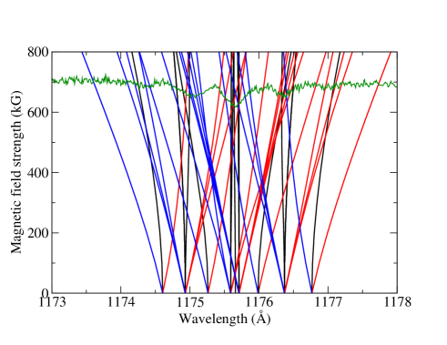
Figure 7: "Spaghetti diagram" showing wavelengths of individual magnetic subcomponents of the C iii sextet at 1175 Å as a function of magnetic field strength, computed as a partial Paschen-Back case. Subcomponents are colour-coded as blue $\sigma$ (blue), $\pi$ (black), and red $\sigma$ (red). The COS flux spectrum (green) is plotted with the continuum set at about 700 kG to show how main line features correspond with clustering of magnetic subcomponents.

The Si ii line at 1265 Å (Figure 4) is one of three resonance lines formed by the 3p ²P^o to 3d ²D transition. Two of the three lines nearly coincide at 1264.730 (strong) and 1265.023 Å (weak). The effect of the partial Paschen-Back effect is to shift all the components of the weaker line towards the blue, and those of the stronger line towards the red, so that radial velocities measured with the $\pi$ or $\sigma$ components of the stronger line in a field near 600 kG will be systematically red shifted from radial velocities measured with lines unaffected by the partial Paschen-Back effect, such as those from the Si iv doublet at 1400 Å. However, the normal Zeeman effect is not a bad approximation at 600 kG, and models of this feature with zeeman.f fit reasonably well assuming a field structure with $\langle|B|\rangle\approx 550$ kG (see Fig. 4).

As discussed above, because the partial Paschen-Back splitting of lines is not implemented in our line synthesis code, we cannot produce an accurate model of the C iii  1175 Å multiplet. Therefore, we have computed the variation of the line splitting as a function magnetic field strength up to 800 kG using gidi.f. Below about 200 kG, the splitting of the individual lines of the multiplet follows closely the prediction of the Zeeman theory. However, by about 600 kG, the splitting is converging on the Paschen-Back limit. In fact, the computed splitting at 600 kG quite closely resembles the observed multiplet, with five groups of line components whose centroids coincide almost exactly with the positions of the observed components, and that agree qualitatively with the relative strengths of those components (Fig. 7).

3.3.8 H in the optical spectrum

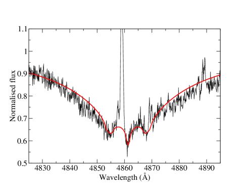
Figure 8: H$\beta$ from UVES spectrum of CC Cet (black) with overplotted fit to line core assuming approximately dipolar magnetic field with $\langle|B|\rangle=620$ kG. The Zeeman triplet is clearly detected in spite of strong emission from the M dwarf secondary star.

The archival UVES spectra cover the entire Balmer spectrum in the visible with resolving power of about 20 000 and S/N of roughly 15–20. Balmer lines H$\alpha$ to H$\epsilon$ are clearly visible in the spectra. We have examined the cores of these lines for evidence of the magnetic field of CC Cet. Because of the low S/N and the presence of emission lines from the M dwarf companion, especially strong in H$\alpha$ and H$\beta$, the magnetic splitting of the Balmer lines by the 700 kG field is not immediately obvious, and was missed in searches for magnetic fields in the analysis of the SPY survey (Napiwotzki et al., 2020; Koester et al., 2009). However, if we smooth the UVES spectra slightly and shift the two spectra to the same stellar radial velocity framework, the superposed H$\beta$ lines reveal fairly clear Zeeman triplet structure, with splitting that agrees closely with that expected from the ultraviolet lines. One spectrum with a model fit is shown in Figure 8.

3.3.9 Rotation velocity

A remarkable feature of both the Si iii 1300 Å and Si iv 1400 Å lines is that the $\pi$ components appear to be broadened beyond the point expected from the instrumental resolution. The $\pi$ components of each line are not broadened by a variation of values of the local magnetic field strength $B$ over the visible hemisphere, so the broadening may instead be due to a rapid rotation of the white dwarf.

Measuring the cleanest $\pi$ components, we find a full width half maximum of about $\approx 60$ km s^-1  and a full width at the continuum of $\approx 80$ km s^-1. CC Cet is a short-period binary system with an M4.5 main sequence star, and thus orbital motion during an exposure may be contributing to the broadening. The velocity semi-amplitude of the M dwarf is about 120 km s^-1(Saffer et al., 1993). The white dwarf has a mass very close to twice that of the M dwarf, so the velocity semi-amplitude is about 60 km s^-1, with the full range being covered in about 3.5 h. During a single 0.5 h COS exposure, the radial velocity of the white dwarf could therefore change by as much as 25 km s^-1. The lines are additionally broadened by the resolving power of the instrument ($\approx 20$ km s^-1) and a small wavelength spread due to the partial Paschen-Back effect ($\approx 9$km s^-1). Summing those factors in quadrature, we find that an additional rotational broadening of $v\sin i\simeq 30-40$ km s^-1 is required to match the shape and width of the observed line profile. As the contribution from the orbital velocity is an upper limit, it is unlikely that $v\,\sin\,i$ is actually much smaller than 40 km s^-1. With this lower limit to $v_{\rm eq}\sin i$ and the radius of CC Cet, we can obtain an upper limit to the spin period $P=2\pi R/v_{\rm eq}\la 2\pi R/v_{\rm eq}\sin i\approx 2000$ s. Given that there are small changes in the magnetic field strength and line depth between spectra, which we infer to be due to different viewing angles of an inhomogenous surface, the rotation period cannot be much shorter than the exposure time of the observations (1865 s) otherwise the variations in field strength would have been smeared out over multiple rotations.

The spin period/orbital period ratio of CC Cet is therefore $\approx 0.05$, consistent with the bulk of the intermediate polars with spin and orbital period measurements (Bernardini et al., 2017). The difference in the line profiles between the two spectra indicate that the magnetic field axis is inclined to the rotation axis and/or the metals are not evenly distributed across the white dwarf surface, so it may be possible to measure the rotation period from high cadence, high signal photometry or spectroscopy. No rotation signal is detected in the TESS light curve, but the red TESS bandpass is dominated by the M dwarf and may not be sensitive to subtle flux variations from the white dwarf. We attempted to produce time-series spectroscopy from the COS data using the costools splittag routine to split the time-tag files into 30 s bins, but the S/N became too low to reliably measure any periodic flux or absorption line variation with a 99.9 per cent false alarm probability limit of $\approx 0.31$ per cent and $\approx 0.28$ per cent for the 2018 Feb and 2018 Jul spectra respectively.

3.3.10 Results of the magnetic analysis

The following conclusions can be drawn from our magnetic modelling efforts. (1) The typical value of $\langle|B|\rangle$ on CC Cet is about 600–700 kG. This value may differ by $\approx 50-100$ kG between the two COS observations. The deduced value of the field appears to be generally consistent with the splitting of all photospheric lines in the spectrum, although some observed lines (such as the sextet of lines of C iii at 1175 Å), are split by the partial Paschen-Back effect in ways that our modelling code cannot reproduce accurately. (2) The fact that the centre of the 1402 Å line reaches almost to the continuum shows that there are no large regions of field strength close to zero on the visible surface. These facts are consistent with, but do not strongly require, a roughly dipole-like field, similar to those found in some other low field magnetic white dwarfs that have been modelled in detail (e.g. WD 2047+372: see Landstreet et al., 2017). (3) CC Cet has $v\sin i\approx 40$ km s^-1, and therefore has a rotation period ≲2000 s, but not much shorter than that due to the differences seen between the two 1865 s exposures.

3.4 X-ray Analysis

Since there were too few X-ray events to perform any sort of spectral analysis, in order to understand the source X-ray luminosity that might have given rise to a weak signal we used the PIMMS software version 4.11 to convert between pn and MOS count rates and incident X-ray flux. This was done for the APEC optically-thin plasma radiative loss model (Foster et al., 2012) for the solar abundances of Asplund et al. (2009) and an intervening hydrogen column density of $2\times 10^{20}$ cm^-2. The latter was estimated from the distance of 121 pc (Gaia Collaboration et al., 2018) and interpolation within the neutral hydrogen column density compilations of Linsky et al. (2019) and Gudennavar et al. (2012).

The resulting X-ray luminosities in the 0.3–10 keV band corresponding to the observed pn and MOS count rates are illustrated as a function of isothermal plasma temperature in Figure 9. The luminosities for a typical active stellar coronal temperature of $10^{7}$ K are also listed in Table 1. Sensitivity of the results to the adopted absorbing column was examined by computing the analogous luminosities for values of $N_{\mathrm{H}}$ lower and high by a factor of two, while sensitivity to metallicity was checked by computing luminosities for metallicity reduced by a factor of two. These cases are also illustrated in Figure 9. By far the largest uncertainty is in the estimate of the X-ray count rates. Luminosities derived from the MOS data appear larger than those from pn, but again the uncertainties overlap for most of the temperature range expected for active stellar coronae.

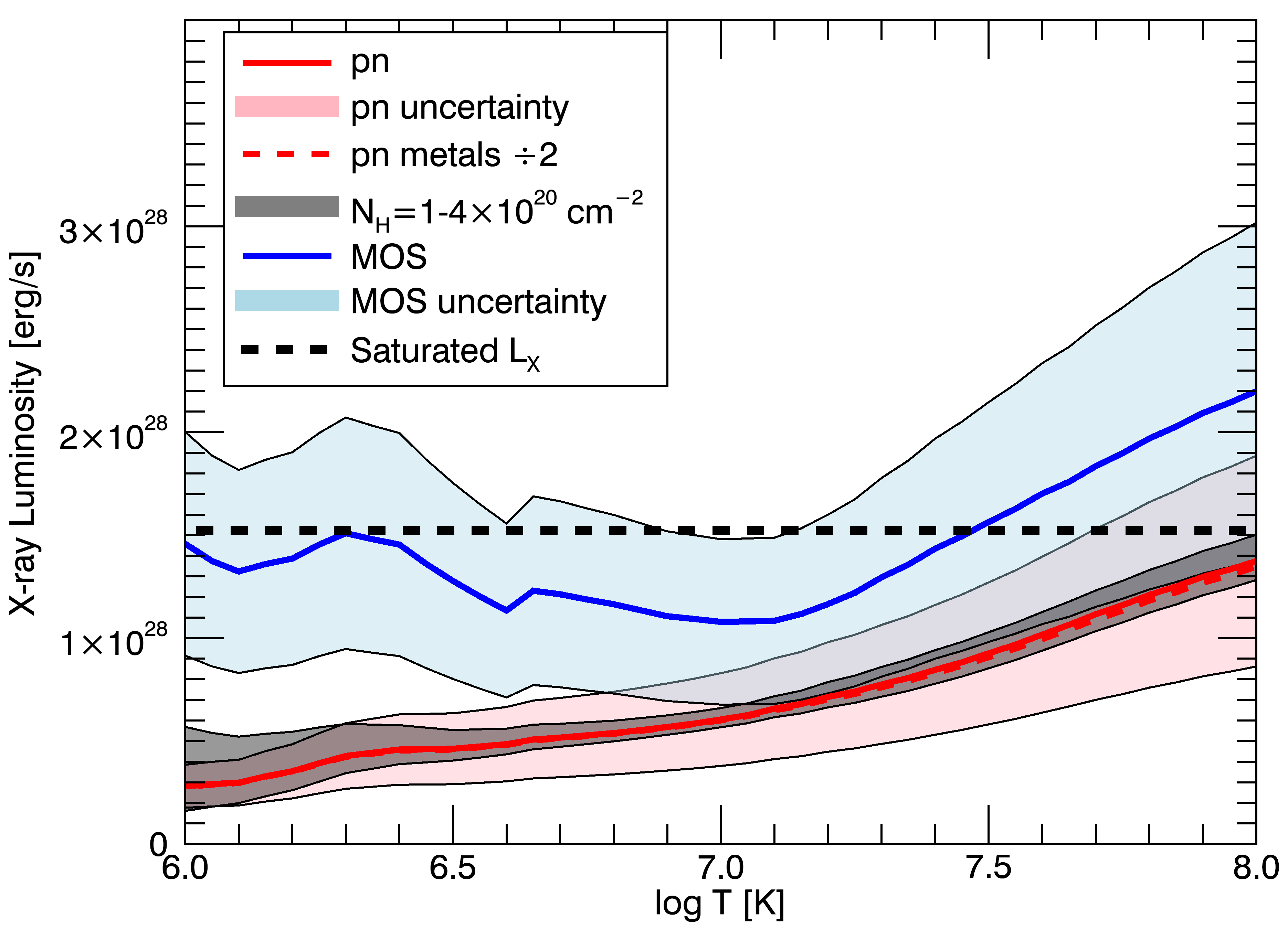
Figure 9: The X-ray luminosities obtained from XMM-Newton pn and MOS count rates assuming the X-ray signal originates in a hot isothermal collision-dominated optically-thin plasma. The derived luminosities are shown as a function of isothermal plasma temperature. Uncertainty ranges due to Poisson statistics in the observed count rates, and to uncertainties in the intervening interstellar medium absorbing column are indicated by shaded regions. The sensitivity to plasma metallicity is very low and indicated for the pn case only. The saturated coronal X-ray emission level for a star of the spectral type of the CC Cet secondary is also illustrated.

Also shown in Figure 9 is the canonical X-ray saturation luminosity, $L_{\mathrm{X}}/L_{\mathrm{bol}}=10^{-3}$, corresponding to an M4.5 V star with a luminosity of $0.0040\mathrm{L}_{\odot}$ (Pecaut & Mamajek, 2013). Our very tentative detection of CC Cet then lies essentially at the saturation limit. This is expected since the orbital period of the binary, and presumably the rotation period of the secondary M dwarf assuming tidal synchronization, is well into the saturated regime that sets in at rotation periods shorter than approximately 20 days for a mid-M dwarf (e.g. Wright et al., 2011).

4 Discussion

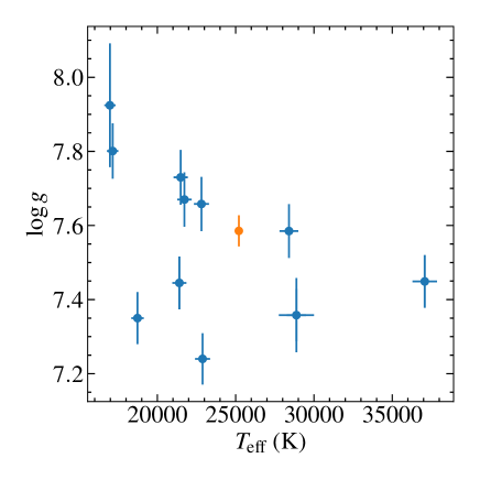
Figure 10: Atmospheric parameters of the white dwarfs in PCEBs observed with HST/COS, demonstrating that CC Cet (orange) is not an outlier in either $T_{\mathrm{eff}}$ or $\log g$.

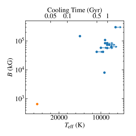
Figure 11: Temperatures and magnetic field strengths of known magnetic white dwarfs in PCEBs compiled by Ferrario et al. (2015) and Parsons et al. (2021) (blue) compared with CC Cet (orange). An approximate cooling time scale is given on the top axis. CC Cet is clearly an extreme outlier in both $T_{\mathrm{eff}}$ and $B$.

4.1 CC Cet in context

Along with CC Cet, program 15189 observed 9 other PCEBs containing a white dwarf and an M dwarf with the same COS setup. Archival COS G130M spectra of three additional PCEBs exhibiting metal absorption lines are also available (Programs 12169,12474,12869). Although a full analysis of these observations will be left for a future publication, we can use them to estimate an occurrence rate for magnetic PCEBs. All the other 12 white dwarf spectra show metal absorption lines, with no detectable magnetic field ($\langle|B|\rangle$ $\lesssim 100$ kG). Although the PCEBs were selected for practicality of observation, rather than to provide an unbiased sample, a comparison of the white dwarf atmospheric parameters (Figure 10) demonstrates that CC Cet is typical of the sample. Using the astropy.stats.binned_binom_proportion function we calculate an occurrence rate for magnetic white dwarfs of $7.7^{+14}_{-2.5}$ per cent, where the uncertainties are the $1\sigma$ confidence boundaries. This stands in stark contrast to the 0/1735 ($<0.11$ per cent) and 2/1200 ($0.17^{+0.22}_{-0.05}$ per cent) rates found by Liebert et al. (2015) and (Silvestri et al., 2007) respectively. The reason for the discrepancy is probably the different waveband used here to the two previous studies: the ultraviolet wavelength range is riddled with sharp metal absorption lines that are sensitive tracers of even relatively low fields, which will go unrecognised in low-resolution optical spectra such as those obtained by the Sloan Digital Sky Survey, and are difficult to detect even in high-resolution spectra of the Balmer lines (see Section 3.3.8, Figure 8). We note that the fraction of intermediate polars among the CVs in the nearly complete 150 pc sample of Pala et al. (2020) is $3/42$ or $7.1^{+6.6}_{-2.2}$ per cent, i.e. consistent with the incidence of magnetic white dwarfs in the COS PCEB sample derived above.

Figure 11 compares CC Cet with the effective temperatures and magnetic field strengths of the magnetic PCEBs compiled by Ferrario et al. (2015) and the latest discoveries by Parsons et al. (2021). CC Cet is clearly an extreme outlier, being both much hotter (and therefore younger) than the rest of the sample and having a much weaker magnetic field strength, even in comparison to the other confirmed pre-intermediate polar SDSS J030308.35+005444.1. CC Cet is an outlier by $\approx 6\sigma$ in both $\log(B)$ and $T_{\mathrm{eff}}$(where the stars that only have upper limits on $T_{\mathrm{eff}}$ were treated as being at the upper limit).

4.2 Formation and evolution

4.2.1 Formation

Invoking a common origin for the magnetic white dwarfs in Figure 11 would imply a large and thus-far undetected population filling the parameter space in between CC Cet and the rest of the sample. We speculate that it is instead more likely that the CC Cet magnetic field was formed via a different pathway to those of the previously known pre-polars. Such a pathway must consistently explain the low but non-zero occurrence rate of magnetic white dwarfs in PCEBs, as well as the high rotation rate and low mass of the CC Cet white dwarf. Here we discuss the various proposed formation scenarios for magnetic white dwarfs and their applicability to CC Cet:

Spin up from accretion: The crystallization/spin up model (Isern et al., 2017; Schreiber et al., 2021) successfully reproduces the existing examples of cool, high-field pre-polars. However, this model require the system to have undergone a period of mass transfer via Roche lobe overflow. As we will discuss in Section 4.2.2, the CC Cet secondary will not fill its Roche lobe and start mass transfer for many Gyr. Furthermore, the system is too young for the white dwarf core to have adequately crystallized. Our measured mass for the CC Cet white dwarf, $0.441\pm 0.008$ $\mathrm{M}_{\odot}$, indicates that it may be a He-core white dwarf (Driebe et al., 1998; Althaus et al., 2013), and thus may lack altogether the core chemical stratification necessary to generate a dynamo via convection.

Fossil Field: In the fossil field model, the progenitor of the white dwarf is an Ap/Bp star with the magnetic field in place before the common envelope. Whilst we cannot conclusively rule this pathway out, there are several issues. Firstly, the formation of the Ap/Bp star is thought to be due to a main sequence stellar merger (Braithwaite & Spruit, 2004), so the average masses of the progenitor stars, and by extension their white dwarf remnants, should be higher than non-magnetic objects (Ferrario et al., 2020). CC Cet’s mass is instead lower than the average masses of both PCEBs and CVs (Zorotovic et al., 2011). The fossil field pathway also provides no explanation for the high rotation rate of the CC Cet white dwarf.

Common envelope dynamo: Briggs et al. (2018) proposed a model whereby a weak initial field is wound up by differential rotation between the two stellar components in a common envelope. Whilst Belloni & Schreiber (2020) found that this model was unable to predict the observed magnetic white dwarf population, it may still be relevant for rare objects such as CC Cet. The fact that the CC Cet white dwarf is already rotating with a period similar to those seen in intermediate polars may also hint at unusual dynamical interactions in the common envelope. Using Equation 1 of Briggs et al. (2018) and assuming that the current orbital period of CC Cet is close to the initial post-common envelope orbital period, we find a predicted field strength of $\approx 20$ MG, roughly 30 times the measured value. The common envelope dynamo model as it stands cannot therefore fully explain the CC Cet system, but could still, at least conceptually, provide a formation scenario for the magnetic white dwarfs in CC Cet and the intermediate polars. However, any future extension of this model will also have to explain why most systems emerging from a common envelope are not magnetic (Fig. 10).

4.2.2 Future of CC Cet

The future of CC Cet was first modelled by Schreiber & Gänsicke (2003). They found that the companion will fill its Roche-lobe and start mass transfer onto the white dwarf, becoming a cataclysmic variable once the system has evolved down to an orbital period of $P_{\mathrm{orb}}\simeq 2$ h in $\simeq 18$ Gyr.

Here we improve on those calculations using the state-of-the-art stellar evolution code Modules for Experiments in Stellar Astrophysics (MESA v.12778, Paxton et al., 2011; Paxton et al., 2013, 2015, 2018, 2019). The standard model of evolution for CVs states that the orbital period is reduced via angular momentum losses driven by gravitational wave radiation (Paczyński, 1967) and magnetic braking generated by the secondary (donor) star (Verbunt & Zwaan, 1981; Rappaport et al., 1983; Mestel & Spruit, 1987; Kawaler, 1988; Andronov et al., 2003). The low mass of the donor star in CC Cet indicates that it is fully convective, so magnetic braking is not active and the reduction of CC Cet’s orbit is driven only by the angular momentum loss via emission of gravitational waves.

For our simulations we adopt an initial orbital period of 0.287 d and treat the white dwarf as a point source with a mass 0.44 $\mathrm{M}_{\odot}$(Table 2). We assumed that the white dwarf retains none of the accreted mass (mass_transfer_beta = 1.0, where the typical assumption is that the accreted mass is ejected in classical nova eruptions) and adopted the $M_{\rm donor}=0.18\pm 0.05$ $\mathrm{M}_{\odot}$ secondary mass from Saffer et al. (1993). We ran the simulations with two different prescriptions for the gravitational wave radiation: (1) the classical prescription dictated by Einstein’s quadrupole formula (Paczyński, 1967) and (2) the calibrated version, which reproduces the observed masses and radii of the donors in cataclysmic variables (Knigge et al., 2011). The simulations were ended when the mass of the donor reached the brown dwarf mass limit ($\mbox{{star\_mass\_min\_limit}}=0.08\,\mbox{$\mathrm{M}_{\odot}$}$).

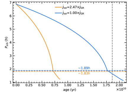
Figure 12: MESA simulations adopting angular momentum loss via gravitational wave radiation using the classical prescription (Paczyński, 1967, blue) and the calibrated version (Knigge et al., 2011, orange). Our simulations show that CC Cet will start mass transfer from the secondary onto the white dwarf (i.e. become a cataclysmic variable) in the next 17.7 Gyr and 7.2 Gyr, for the classical and the calibrated versions of gravitational radiation, respectively. The vertical dashed line shows the calculations performed by Schreiber & Gänsicke (2003) using the classical prescription, which is slightly longer than in our simulations. The system will have an orbital period shorter than 2 hr when the accretion starts (dashed lines.)

The results of our simulations confirm that the final fate of CC Cet is to become an intermediate polar. The system will start to transfer mass at a low rate of $\simeq 3.5\times 10^{-11}$ $\mathrm{M}_{\odot}$/yr ($\simeq 10^{-10}$ $\mathrm{M}_{\odot}$/yr) in roughly 17.7 Gyr (7.2 Gyr) for the classical (calibrated) version of gravitational radiation. The system will have an orbital period of $\approx 1.89$ ($\approx 1.83$) h when the accretion starts (Figure 12). The accretion rate will slightly decrease while the system continues shrinking, until the mass of the donor reaches a mass of 0.08 $\mathrm{M}_{\odot}$ at an orbital period of $\simeq 1.14$ h ($\simeq 1.24$ h).

Norton et al. (2004) modelled the magnetic moment of intermediate polars given their measured spin period to orbital period ratios. Given that we know the magnetic moment of CC Cet ($\mu_{1}=B\,R^{3}\approx 1.35\times 10^{33}$ G cm^-3), we can use their Figure 2 to estimate the white dwarf spin period when it reaches the orbital period minimums calculated above. We find equilibrium spin periods of $\simeq 1.7$ min ($\simeq 1.9$ min) for orbital periods of $\simeq 1.14$ h ($\simeq 1.24$ h), comparable to the spin period of V455 And, an intermediate polar near the orbital period minimum (Araujo-Betancor et al., 2005; Bloemen et al., 2013).

4.3 M dwarf wind

As mass-transfer by Roche lobe overflow has not yet begun in the CC Cet system, the origin of the metals in the white dwarf atmosphere is most likely the stellar wind of the M dwarf companion. Debes (2006) has demonstrated that such wind accreting systems can be used to quantify the wind mass-loss rates of M dwarfs, which is otherwise extremely difficult to measure (see Wood et al. 2021 for a summary of the current state of the art). Debes (2006) assumed that the non-magnetic white dwarfs in their sample accreted via the Bondi-Hoyle process (Bondi & Hoyle, 1944), where the white dwarf gathers a fraction of the stellar wind in proportion to its mass and the wind velocity. Webbink & Wickramasinghe (2005) demonstrated that for binaries containing white dwarfs with high (10s of MG, i.e pre-polars) magnetic fields, the energy density of the magnetic field is much stronger than that of the wind down to the surface of the secondary, and thus the white dwarf accretes all of the wind emitted. CC Cet is an intermediate case, where the magnetic field is not strong enough to accrete all of the wind but nevertheless gathers wind from a wider radius than the Bondi-Hoyle process. Following the model from Section 6 of Webbink & Wickramasinghe (2005), the wind will be accreted inside of a critical radius $r_{\mathrm{crit}}$ from the white dwarf where the energy density of the magnetic field exceeds that of the wind:

$$\frac{\left(B_{0}\left(\frac{\displaystyle r_{\mathrm{wd}}}{\displaystyle r_{\mathrm{crit}}}\right)^{3}\right)^{2}}{8\pi}=u_{0}\left(\frac{r_{\mathrm{md}}}{a-r_{\mathrm{crit}}}\right)^{2}$$ (3)

Where $B_{0}$ is the strength of the magnetic field at the white dwarf surface, $u_{0}$ the energy density of the wind at the secondary surface, $a$ the orbital separation, and $r_{\mathrm{wd}}$ and $r_{\mathrm{md}}$ the radii of the primary and secondary, respectively. Taking the average of our two magnetic field measurements and adopting a secondary radius of $r_{\mathrm{md}}=0.243$ $\mathrm{R}_{\odot}$ from the latest version of the tables from Pecaut & Mamajek (2013), we numerically solve equation 3 to find a critical radius of $\approx$ 1.2 $\mathrm{R}_{\odot}$, 75 per cent of the orbital radius and roughly twice the Bondi radius. Assuming (incorrectly, but close enough for our purposes) that the M dwarf emits wind uniformly in all directions, the accretion rate of wind siphoned onto the white dwarf $\dot{M}_{\mathrm{wd}}$ is:

$$\dot{M}_{\mathrm{wd}}=\dot{M}_{\mathrm{wind}}\left(\frac{r_{\mathrm{crit}}}{a}\right)^{2}$$ (4)

To calculate $\dot{M}_{\mathrm{wd}}$, we take the average of our measured Si abundances and calculate an accretion rate assuming that the atmosphere is in accretion diffusion equilibrium (Koester, 2010), using the diffusion timescales from the Montreal White Dwarf Database. We then assumed that the wind has Solar abundances, so scaled the Si accretion rate to the total accretion rate via the Si mass fraction measured by Asplund et al. (2009), arriving at an accretion rate onto the white dwarf of $\approx 7.3\times 10^{9}$ g s^-1. Via equation 4, we therefore infer a wind mass loss rate $\dot{M}_{\mathrm{wind}}$ of $\approx 1.3\times 10^{10}$ g s^-1 or $\approx 2\times 10^{-16}$ $\mathrm{M}_{\odot}$ yr^-1. Repeating the calculation with only Bondi-Hoyle accretion in effect results in an inferred wind rate approximately an order of magnitude higher. These values are comparable to the wind mass loss rates found by (Debes, 2006).

X-ray observations may also be used to place constraints on the wind mass loss rate. Although the weak X-ray detection at CC Cet can be satisfactorily accounted for by coronal emission (Section 3.4), it is still possible that some fraction of the signal could be due to accretion onto the white dwarf. The maximum X-ray luminosity that can be extracted from accretion by conversion of gravitational potential energy to X-rays is $L_{\mathrm{X}}\leq GM_{\mathrm{wd}}\dot{M}/R_{\mathrm{wd}}$. For an X-ray luminosity of $L_{\mathrm{X}}\sim 10^{28}$ erg s^-1, and the white dwarf mass and radius derived in Sect. 3.1, the corresponding maximum mass accretion rate is $\sim 3\times 10^{-15}\mbox{$\mathrm{M}_{\odot}$}$ yr^-1. This is of the same order of magnitude as estimates of the mass loss rate for the moderately active mid-M dwarf Proxima Centuri (e.g. Wood, 2018; Wargelin & Drake, 2002). Since the white dwarf is unlikely to accrete a majority of the stellar wind, a more reasonable accretion efficiency of $\sim 10$% would imply a mass loss rate of $3\times 10^{-14}M_{\odot}$ yr^-1, which is similar to that of the Sun. As this is two orders of magnitude higher than the mass loss rate estimated from the photospheric metal absorption lines, we retain the former value as the final wind mass loss rate.

5 Conclusions

We have detected a 600–700 kG magnetic field on the white dwarf component of the detached PCEB CC Cet, classifying it as a pre-intermediate polar. Analysis of HST COS spectra demonstrates that the white dwarf is accreting the stellar wind of its M4.5–5 companion inhomogenously over its surface, and that the axis of the magnetic field is likely offset from the spin axis of the white dwarf. The white dwarf has a relatively low mass of $0.441\pm 0.008$ $\mathrm{M}_{\odot}$, and is rotating with a period of $\la 2000$ s, which is much faster than the $6.88233\pm 0.00045$ h binary orbital period and consistent with the high spin period to orbital period ratios of intermediate polars.

CC Cet is by far the youngest and has the weakest field of all known magnetic white dwarfs in detached PCEBs, being a 6 $\sigma$ outlier in both $T_{\mathrm{eff}}$ and $B$. Using MESA stellar evolution models, we show that the secondary star will not start mass transfer for at least 7 Gyr, and is so far from filling its Roche lobe that it cannot have undergone a period of mass transfer in the past, unlike the rest of the known pre-polars. The CC Cet magnetic field therefore cannot have formed via mass transfer, ruling out the formation pathway proposed by Schreiber et al. (2021) for the pre-polars. The CC Cet magnetic field must instead have formed either before or during the common envelope phase, although neither the fossil field or common envelope interaction models provide a complete explanation of the observed white dwarf properties.

The occurrence rate of magnetic to non-magnetic white dwarfs in the available sample of PCEBs with ultraviolet spectra is consistent with the fraction of intermediate polars among CVs in the 150 pc sample. However, with only one known example in a relatively small sample, we can place only limited constraints on both the true occurrence rate and formation pathway of CC Cet-like systems. The online catalogue of white dwarf plus main sequence binaries compiled by Rebassa-Mansergas et al. (2012) contains 66 objects with GALEX FUV magnitudes $<16$, roughly the limit where ultraviolet spectroscopy of similar precision to CC Cet ($FUV=14.03$ mag) can be obtained. The periods of most of these targets are currently unconstrained, so in many cases the binary separation may be too large for stellar wind accretion to form the strong absorption lines required to search for magnetic fields. If periods for these systems can be measured, and are favourable for wind accretion, then a factor 2–3 increase in the number of PCEBs with ultraviolet spectra may be achievable, further constraining the occurrence rate and/or discovering new examples of magnetic systems.

6 Data Availability

All of the observational data used in this paper is publicly available and can be retrieved from the relevant online archives (see Table 3).

Appendix A Supplementary Material

Table 3: Summary of spectroscopic observations of CC Cet. Dataset numbers are given for retrieval from MAST (https://archive.stsci.edu/hst/), the XMM-Newton Science Archive (http://nxsa.esac.esa.int/nxsa-web/#home) and or the ESO Archive Science Portal (http://archive.eso.org/scienceportal/home).

Date	Instrument	Grating	Central Wavelength (Å)	Start Time (UT)	Total Exposure Time (s)	Dataset
HST
2018-02-02	COS	G130M	1291	23:50:53	1865	LDLC01010
2018-07-22	COS	G130M	1291	05:40:51	1865	LDLC51010
XMM
2018-02-01	–	–	–	22:48:07	9500	0810230101
2018-02-01	–	–	–	22:48:07	16800	0810231301
VLT
2001-02-07	UVES	–	5635	01:27:42.810	600	ADP.2020-09-01T15:53:01.123
2001-02-07	UVES	–	3922	01:27:44.233	600	ADP.2020-09-01T15:53:01.174
2001-02-08	UVES	–	3922	01:36:22.407	600	ADP.2020-09-01T15:54:42.325
2001-02-08	UVES	–	5635	01:36:21.194	600	ADP.2020-09-01T15:54:42.356

Table 4: Interstellar absorption lines identified in the COS spectrum of CC-Cet. These lines are narrower than the white dwarf’s photospheric absorption lines because they are not affected by the rotational broadening of the white dwarf.

Ion	wavelength (Å; vacuum)
C ii	1334.532, 1335.703
N i	1134.165, 1134.415, 1134.980, 1199.549, 1200.224, 1200.711
O ii	1302.168
Si ii	1190.416, 1193.289, 1260.421, 1304.372
S ii	1250.586, 1253.812, 1259.520

References

- Althaus et al. (2013) Althaus L. G., Miller Bertolami M. M., Córsico A. H., 2013, A&A, 557, A19
- Andronov et al. (2003) Andronov N., Pinsonneault M., Sills A., 2003, ApJ, 582, 358
- Araujo-Betancor et al. (2005) Araujo-Betancor S., et al., 2005, A&A, 430, 629
- Asplund et al. (2009) Asplund M., Grevesse N., Sauval A. J., Scott P., 2009, ARA&A, 47, 481
- Bell et al. (2019) Bell K. J., et al., 2019, arXiv e-prints, p. arXiv:1910.04180
- Belloni & Schreiber (2020) Belloni D., Schreiber M. R., 2020, MNRAS, 492, 1523
- Bergeron et al. (1995) Bergeron P., Wesemael F., Beauchamp A., 1995, PASP, 107, 1047
- Bernardini et al. (2017) Bernardini F., de Martino D., Mukai K., Russell D. M., Falanga M., Masetti N., Ferrigno C., Israel G., 2017, MNRAS, 470, 4815
- Bloemen et al. (2013) Bloemen S., Steeghs D., De Smedt K., Vos J., Gänsicke B. T., Marsh T. R., Rodriguez-Gil P., 2013, MNRAS, 429, 3433
- Bondi & Hoyle (1944) Bondi H., Hoyle F., 1944, MNRAS, 104, 273
- Braithwaite & Spruit (2004) Braithwaite J., Spruit H. C., 2004, Nat, 431, 819
- Briggs et al. (2018) Briggs G. P., Ferrario L., Tout C. A., Wickramasinghe D. T., 2018, MNRAS, 481, 3604
- Capitanio et al. (2017) Capitanio L., Lallement R., Vergely J. L., Elyajouri M., Monreal-Ibero A., 2017, A&A, 606, A65
- Condon & Shortley (1935) Condon E. U., Shortley G. H., 1935, The Theory of Atomic Spectra. Cambridge University Press
- Debes (2006) Debes J. H., 2006, ApJ, 652, 636
- Dekker et al. (2000) Dekker H., D’Odorico S., Kaufer A., Delabre B., Kotzlowski H., 2000, in Iye M., Moorwood A. F., eds, Society of Photo-Optical Instrumentation Engineers (SPIE) Conference Series Vol. 4008, Optical and IR Telescope Instrumentation and Detectors. pp 534–545
- Driebe et al. (1998) Driebe T., Schoenberner D., Bloecker T., Herwig F., 1998, A&A, 339, 123
- Feinstein et al. (2019) Feinstein A. D., et al., 2019, PASP, 131, 094502
- Ferrario et al. (1995) Ferrario L., Wickramasinghe D., Bailey J., Buckley D., 1995, MNRAS, 273, 17
- Ferrario et al. (2015) Ferrario L., de Martino D., Gänsicke B. T., 2015, Space Sci. Rev., 191, 111
- Ferrario et al. (2020) Ferrario L., Wickramasinghe D., Kawka A., 2020, Advances in Space Research, 66, 1025
- Fitzpatrick (1999) Fitzpatrick E. L., 1999, PASP, 111, 63
- Fontaine et al. (2001) Fontaine G., Brassard P., Bergeron P., 2001, PASP, 113, 409
- Foreman-Mackey (2016) Foreman-Mackey D., 2016, The Journal of Open Source Software, 1, 24
- Foreman-Mackey et al. (2013) Foreman-Mackey D., Hogg D. W., Lang D., Goodman J., 2013, PASP, 125, 306
- Foster et al. (2012) Foster A. R., Ji L., Smith R. K., Brickhouse N. S., 2012, ApJ, 756, 128
- Gaia Collaboration et al. (2018) Gaia Collaboration et al., 2018, A&A, 616, A1
- Gänsicke et al. (2004) Gänsicke B. T., Araujo-Betancor S., Hagen H.-J., Harlaftis E. T., Kitsionas S., Dreizler S., Engels D., 2004, A&A, 418, 265
- Green et al. (2012) Green J. C., et al., 2012, ApJ, 744, 60
- Gudennavar et al. (2012) Gudennavar S. B., Bubbly S. G., Preethi K., Murthy J., 2012, ApJS, 199, 8
- Holberg & Bergeron (2006) Holberg J. B., Bergeron P., 2006, AJ, 132, 1221
- Inight et al. (2021) Inight K., Gänsicke B. T., Breedt E., Marsh T. R., Pala A. F., Raddi R., 2021, MNRAS, 504, 2420
- Isern et al. (2017) Isern J., García-Berro E., Külebi B., Lorén-Aguilar P., 2017, ApJ, 836, L28
- Kővári et al. (2021) Kővári Z., et al., 2021, arXiv e-prints, p. arXiv:2103.02041
- Kawaler (1988) Kawaler S. D., 1988, ApJ, 333, 236
- Knigge et al. (2011) Knigge C., Baraffe I., Patterson J., 2011, ApJS, 194, 28
- Koester (2010) Koester D., 2010, Memorie della Societa Astronomica Italiana,, 81, 921
- Koester et al. (2009) Koester D., Voss B., Napiwotzki R., Christlieb N., Homeier D., Lisker T., Reimers D., Heber U., 2009, A&A, 505, 441
- Koester et al. (2014) Koester D., Gänsicke B. T., Farihi J., 2014, A&A, 566, A34
- Kowalski & Saumon (2006) Kowalski P. M., Saumon D., 2006, ApJ, 651, L137
- Krtička et al. (2019) Krtička J., et al., 2019, A&A, 625, A34
- Lallement et al. (2014) Lallement R., Vergely J. L., Valette B., Puspitarini L., Eyer L., Casagrande L., 2014, A&A, 561, A91
- Lallement et al. (2018) Lallement R., et al., 2018, A&A, 616, A132
- Landi Degl’Innocenti & Landolfi (2004) Landi Degl’Innocenti E., Landolfi M., 2004, Polarization in Spectral Lines. Astrophysics and Space Library Vol. 307, Kluwer, doi:10.1007/978-1-4020-2415-3
- Landstreet (1988) Landstreet J. D., 1988, ApJ, 326, 967
- Landstreet (1992) Landstreet J. D., 1992, A&ARv, 4, 35
- Landstreet et al. (2017) Landstreet J. D., Bagnulo S., Valyavin G., Valeev A. F., 2017, A&A, 607, A92
- Liebert et al. (2005) Liebert J., et al., 2005, AJ, 129, 2376
- Liebert et al. (2015) Liebert J., Ferrario L., Wickramasinghe D. T., Smith P. S., 2015, ApJ, 804, 93
- Lightkurve Collaboration et al. (2018) Lightkurve Collaboration et al., 2018, Lightkurve: Kepler and TESS time series analysis in Python, Astrophysics Source Code Library (ascl:1812.013)
- Linsky et al. (2019) Linsky J. L., Redfield S., Tilipman D., 2019, ApJ, 886, 41
- Lopes de Oliveira et al. (2020) Lopes de Oliveira R., Bruch A., Rodrigues C. V., Oliveira A. S., Mukai K., 2020, ApJ, 898, L40
- Mestel & Spruit (1987) Mestel L., Spruit H. C., 1987, MNRAS, 226, 57
- Napiwotzki et al. (2020) Napiwotzki R., et al., 2020, A&A, 638, A131
- Nebot Gómez-Morán et al. (2011) Nebot Gómez-Morán A., et al., 2011, A&A, 536, A43
- Norton et al. (2004) Norton A. J., Wynn G. A., Somerscales R. V., 2004, ApJ, 614, 349
- Paczyński (1967) Paczyński B., 1967, Acta Astron., 17, 287
- Paczynski & Sienkiewicz (1981) Paczynski B., Sienkiewicz R., 1981, ApJ, 248, L27
- Pala et al. (2020) Pala A. F., et al., 2020, MNRAS, 494, 3799
- Parsons et al. (2013) Parsons S. G., Marsh T. R., Gänsicke B. T., Schreiber M. R., Bours M. C. P., Dhillon V. S., Littlefair S. P., 2013, MNRAS, 436, 241
- Parsons et al. (2021) Parsons S. G., Gänsicke B. T., Schreiber M. R., Marsh T. R., Ashley R. P., Breedt E., Littlefair S. P., Meusinger H., 2021, arXiv e-prints, p. arXiv:2101.08792
- Patterson (1979) Patterson J., 1979, ApJ, 234, 978
- Paxton et al. (2011) Paxton B., Bildsten L., Dotter A., Herwig F., Lesaffre P., Timmes F., 2011, ApJS, 192, 3
- Paxton et al. (2013) Paxton B., et al., 2013, ApJS, 208, 4
- Paxton et al. (2015) Paxton B., et al., 2015, ApJS, 220, 15
- Paxton et al. (2018) Paxton B., et al., 2018, ApJS, 234, 34
- Paxton et al. (2019) Paxton B., et al., 2019, ApJS, 243, 10
- Pecaut & Mamajek (2013) Pecaut M. J., Mamajek E. E., 2013, ApJS, 208, 9
- Potter & Buckley (2018) Potter S. B., Buckley D. A. H., 2018, MNRAS, 473, 4692
- Rappaport et al. (1983) Rappaport S., Joss P. C., Verbunt F., 1983, ApJ, 275, 713
- Rebassa-Mansergas et al. (2010) Rebassa-Mansergas A., Gänsicke B. T., Schreiber M. R., Koester D., Rodríguez-Gil P., 2010, MNRAS, 402, 620
- Rebassa-Mansergas et al. (2012) Rebassa-Mansergas A., Nebot Gómez-Morán A., Schreiber M. R., Gänsicke B. T., Schwope A., Gallardo J., Koester D., 2012, MNRAS, 419, 806
- Reimers & Hagen (2000) Reimers D., Hagen H. J., 2000, A&A, 358, L45
- Reimers et al. (1999) Reimers D., Hagen H. J., Hopp U., 1999, A&A, 343, 157
- Saffer et al. (1993) Saffer R. A., Wade R. A., Liebert J., Green R. F., Sion E. M., Bechtold J., Foss D., Kidder K., 1993, AJ, 105, 1945
- Schmidt et al. (2005) Schmidt G. D., et al., 2005, ApJ, 630, 1037
- Schmidt et al. (2007) Schmidt G. D., Szkody P., Henden A., Anderson S. F., Lamb D. Q., Margon B., Schneider D. P., 2007, ApJ, 654, 521
- Schreiber & Gänsicke (2003) Schreiber M. R., Gänsicke B. T., 2003, A&A, 406, 305
- Schreiber et al. (2021) Schreiber M. R., Belloni D., Gänsicke B. T., Parsons S. G., Zorotovic M., 2021, Nature Astronomy, 5, 648
- Schwope (1990) Schwope A. D., 1990, Reviews of Modern Astronomy, 3, 44
- Schwope et al. (2009) Schwope A. D., Nebot Gomez-Moran A., Schreiber M. R., Gänsicke B. T., 2009, A&A, 500, 867
- Silvestri et al. (2007) Silvestri N. M., et al., 2007, AJ, 134, 741
- Sion et al. (1998) Sion E. M., Schaefer K. G., Bond H. E., Saffer R. A., Cheng F. H., 1998, ApJ, 496, L29
- Sion et al. (2012) Sion E. M., Bond H. E., Lindler D., Godon P., Wickramasinghe D., Ferrario L., Dupuis J., 2012, ApJ, 751, 66
- Somers et al. (1996) Somers M. W., Lockley J. J., Naylor T., Wood J. H., 1996, MNRAS, 280, 1277
- Tappert et al. (2007) Tappert C., Gänsicke B. T., Schmidtobreick L., Mennickent R. E., Navarrete F. P., 2007, A&A, 475, 575
- Toonen et al. (2017) Toonen S., Hollands M., Gänsicke B. T., Boekholt T., 2017, A&A, 602, A16
- Tremblay et al. (2011) Tremblay P.-E., Bergeron P., Gianninas A., 2011, ApJ, 730, 128
- Verbunt & Zwaan (1981) Verbunt F., Zwaan C., 1981, A&A, 100, L7
- Vogel et al. (2007) Vogel J., Schwope A. D., Gänsicke B. T., 2007, A&A, 464, 647
- Wargelin & Drake (2002) Wargelin B. J., Drake J. J., 2002, ApJ, 578, 503
- Webbink & Wickramasinghe (2005) Webbink R. F., Wickramasinghe D. T., 2005, in Hameury J. M., Lasota J. P., eds, Astronomical Society of the Pacific Conference Series Vol. 330, The Astrophysics of Cataclysmic Variables and Related Objects. p. 137
- Wood (2018) Wood B. E., 2018, in Journal of Physics Conference Series. p. 012028 (arXiv:1809.01109), doi:10.1088/1742-6596/1100/1/012028
- Wood et al. (2021) Wood B. E., et al., 2021, arXiv e-prints, p. arXiv:2105.00019
- Wright et al. (2011) Wright N. J., Drake J. J., Mamajek E. E., Henry G. W., 2011, ApJ, 743, 48
- Zorotovic et al. (2011) Zorotovic M., Schreiber M. R., Gänsicke B. T., 2011, A&A, 536, A42