Central kinematics of the Galactic globular cluster M80

Abstract

We use spectra observed with the integral-field spectrograph MUSE to reveal the central kinematics of the Galactic globular cluster Messier 80 (M80, NGC 6093). Using observations obtained with the recently commissioned narrow-field mode of MUSE, we are able to analyse 932 stars in the central 7.5 arcsec by 7.5 arcsec of the cluster for which no useful spectra previously existed. Mean radial velocities of individual stars derived from the spectra are compared to predictions from axisymmetric Jeans models, resulting in radial profiles of the velocity dispersion, the rotation amplitude, and the mass-to-light ratio. The new data allow us to search for an intermediate-mass black hole (IMBH) in the centre of the cluster. Our Jeans model finds two similarly probable solutions around different dynamical cluster centres. The first solution has a centre close to the photometric estimates available in the literature and does not need an IMBH to fit the observed kinematics. The second solution contains a location of the cluster centre that is offset by about 2.4 arcsec from the first one and it needs an IMBH mass of $4600^{+1700}_{-1400}~{}\text{M}_{\odot}{}.$ $N$-body models support the existence of an IMBH in this cluster with a mass of up to $6000~{}\text{M}_{\odot}$ in this cluster, although models without an IMBH provide a better fit to the observed surface brightness profile. They further indicate that the cluster has lost nearly all stellar-mass black holes. We further discuss the detection of two potential high-velocity stars with radial velocities of 80 to 90 $\text{km}\,\text{s}^{-1}$ relative to the cluster mean.

1 Introduction

The cores of globular clusters (GCs) are among the regions with the highest density of stars. With up to $10^{5}$ stars per cubic parsec, they contain a multitude of stellar exotica including millisecond pulsars, rejuvenated and heavy stars in form of blue stragglers, cataclysmic variables, accreting and non-accreting stellar-mass black holes as remnants of high-mass stars, and potentially intermediate-mass black holes (IMBH). IMBHs are a hypothetical class of black holes which would fill the gap between stellar-mass black holes with up to a few tens of solar masses and super-massive black holes in the centres of galaxies with masses ranging from millions to billions of solar masses (Greene et al., 2020). Numerical simulations of globular clusters predict that they can contain a single IMBH with a mass of several thousand solar masses (Arca Sedda et al., 2019), formed by merging stellar-mass black holes with massive stars and binaries or by merging massive stars (e.g. Portegies Zwart et al., 2004; Giersz et al., 2015; Rizzuto et al., 2020). An IMBH could be detected through its influence on stellar kinematics as it will increase the velocity dispersion of stars in the centre of a globular cluster. If there is enough gas in the core of a GC, it could be accreted by the IMBH which could cause detectable radio or X-ray emission if the overall accretion efficiency is not too low (Tremou et al., 2018). The deep gravitational potential of an IMBH should cause a change in the period of millisecond pulsars, which could be detectable if all other accelerations are accurately modelled (Kızıltan et al., 2017; Hénault-Brunet et al., 2020; Abbate et al., 2019). So far, observations have not resulted in a convincing detection of an IMBH in a globular cluster but yielded upper mass limits (see Table 3 in Greene et al., 2020). The recent gravitational-wave signal GW190521 points to a heavy BH remnant with a mass of approx. $140~{}\text{M}_{\odot}{}$ (LIGO Scientific Collaboration and Virgo Collaboration et al., 2020; Abbott et al., 2020), which is at the low-mass end of IMBHs. It is unclear in which environment this merger occurred, but star clusters provide favourable conditions but star clusters provide favourable conditions for the merging of black holes that are more massive than what is predicted by single-star evolution (Abbott et al., 2020).

A challenge in the detection of IMBHs via stellar kinematics lies in the unknown amount and mass of stellar remnants residing near the cluster centres (e.g. Gieles et al., 2018; Zocchi et al., 2019; Mann et al., 2019; Baumgardt et al., 2019; Hénault-Brunet et al., 2020). However, detailed studies of the central cluster kinematics can help to discriminate between the presence of an IMBH and an overdensity of stellar remnants. In case of $\omega$ Cen (NGC 5139), Baumgardt et al. (2019) found using N-body models that the proposed $\approx 45{,}000~{}\text{M}_{\odot}{}$ IMBH (Noyola et al., 2010; Jalali et al., 2012; Baumgardt, 2017) would produce about 20 stars with a radial velocity above the maximum stellar velocity measured in the centre of this cluster, while models with a number of stellar-mass black holes instead of a central IMBH do not contain these high-velocity stars. IMBHs are statistically expected to have companion stars inside their sphere of influence, which would extend over several tenths of arcseconds to a few arcseconds for most clusters. Although the innermost companion of an IMBH in a 10-Gyr-old GC will typically be a neutron star, a massive ($>1~{}\text{M}_{\odot}{}$) white dwarf, or a stellar-mass black hole (MacLeod et al., 2016), which are impossible to observe visually, other companions might be observable. Interactions between the IMBH and stars, e.g. a fly-by, could accelerate stars and cause a proper motion or radial velocity much higher than those of stars that did not interact with the IMBH.

M80 (NGC 6093) is an old Milky Way globular cluster with an age of $13.5\pm 1.0$ Gyr (Dotter et al., 2009). It is located in the direction of the Galactic centre at a heliocentric distance of $8.86\pm 0.55$ kpc (Baumgardt & Hilker, 2018). The cluster core radius is $r_{c}\approx 0.36\,\text{pc}=8$ arcsec (Harris, 1996; Baumgardt & Hilker, 2018). It belongs to the group of dynamically old globular clusters (Ferraro et al., 2012). While scaling relations derived from GC simulations predict an IMBH with a mass of $(3.63\pm 0.95)\times 10^{3}\text{M}_{\odot}$ in M80 (Arca Sedda et al., 2019), an integrated-light study did not find evidence for an IMBH (Lützgendorf et al., 2013). Kamann et al. (2020) studied the kinematics of M80 using radial velocities derived from MUSE data from 2015–2017 and the axisymmetric Jeans model from Watkins et al. (2013). This study found that stars belonging to different chemical populations (as discovered by Dalessandro et al., 2018) rotate differently.

In this paper, we build on the study of Kamann et al. (2020) and use new data from the centremost stars in the cluster obtained with the recently commissioned narrow-field mode of MUSE. We combine this with new MUSE wide-field mode data and updated radial velocity estimates (see Sections 1 and 2) to re-analyse the global kinematics of M80 with a Jeans model and calculate rotation profiles, mass-to-light ratio profiles and infer the mass of a hypothetical IMBH (Section 4). Section 5 presents results derived from $N$-body models and the stars with high radial velocities are described in Section 6. We discuss our results in Section 7 and conclude in Section 8.

2 MUSE Observations

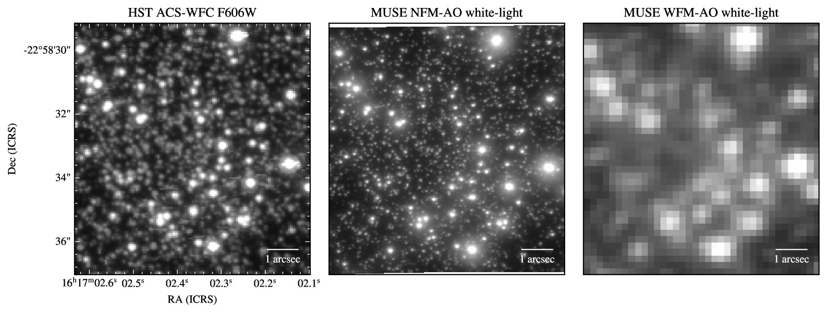
Figure 1: The central 7.5 arcsec by 7.5 arcsec of M80 seen with different instruments. Left: the HST ACS/WFC F606W image (Sarajedini et al., 2007; Anderson et al., 2008), centre: the MUSE NFM white-light image, right: the MUSE WFM-AO white-light image created from the observation with the best seeing (0.4 arcsec). At the cluster distance of 10 kpc, a scale of 1 arcsec corresponds to 0.05 pc. The most complete catalog of this region contains about 1500 stars.

This study makes use of spectroscopic data taken with the Multi Unit Spectroscopic Explorer (MUSE, Bacon et al., 2010) at the Very Large Telescope as part of the GTO programme ‘A stellar census in globular clusters with MUSE’ (PI: S. Dreizler, S. Kamann) which is described in Kamann et al. (2018). MUSE is an optical integral-field spectrograph which is in operation since 2014. Since mid-2019, a new instrument mode (narrow-field mode, NFM) is offered to the community which enables observations with laser tomography adaptive optics to achieve a higher spatial resolution. NFM observations have a higher spatial sampling of 0.025 arcsec in a smaller field of view of 7.5 arcsec by 7.5 arcsec compared to a sampling of 0.2 arcsec in a 1 arcmin by 1 arcmin field of view in wide-field mode (WFM) observations. While the spatial properties differ, the spectral range in both instrument modes covers 4750 to 9300 Å at a constant sampling of 1.25 Å.

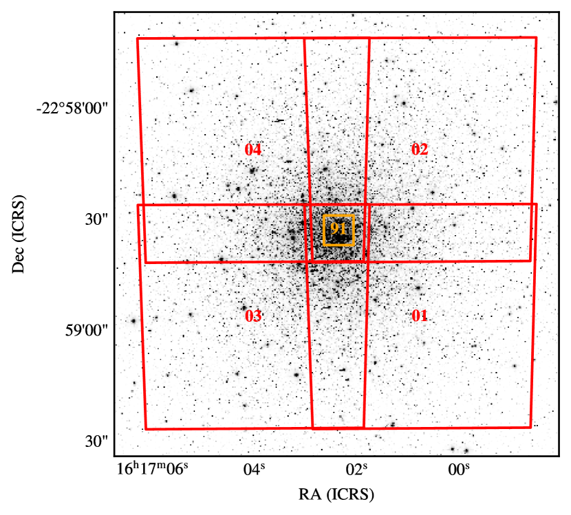
Figure 10: The four MUSE WFM pointings (01–04) and the central NFM pointing (91) on top of the HST ACS image of M80 (Sarajedini et al., 2007; Anderson et al., 2008).

We use all available MUSE observations of M80 taken until February 2020. The data analysed here includes the ten WFM observations used in Kamann et al. (2020), four new WFM observations, and two NFM observations of a single pointing located in the cluster centre. Table 1 lists the five different pointings we observed and the respective instrument mode. The positions of the pointings are shown in Fig. 10.

The main difference of the NFM observations compared to the WFM ones is that we used four instead of three exposures, we did not apply derotator offsets because the natural guide star is off-axis, and the exposure time was 600 s instead of 200 s for each exposure. We used the most recent versions (2.6 and 2.8) of the MUSE data reduction pipeline (Weilbacher et al., 2020) to reduce the additional data compared to Kamann et al. (2020).

Figure 1 compares the image quality of the HST Advanced Camera for Surveys (ACS) Wide Field Channel (WFC) observation using the F606W filter (Sarajedini et al. 2007; Anderson et al. 2008, zoomed on the cluster core), a white-light image created from the MUSE NFM observation, and a MUSE WFM white-light image of the same region derived from the adaptive-optics observation with the best seeing (0.4 arcsec). Clearly, the MUSE WFM observation suffers heavily from crowding, while both the ACS and the MUSE NFM image are less affected. As described in detail in Section 3.1 below, we measure a FWHM of around 40 milliarcseconds (40 mas) in the NFM data, i.e. our spatial resolution is higher than that achieved with ACS-WFC.

3 Extracting and analysing spectra

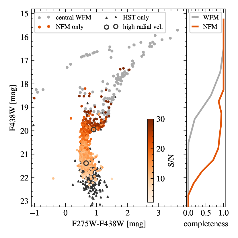
Figure 2: Left panel: CMD of the central region of M80 using the photometric catalog of Dalessandro et al. (2018). Grey dots represent stars with spectra extracted from WFM observations while spectra for the red-orange stars could only be obtained from NFM observations. The colour corresponds to the mean S/N ratio from our two NFM observations. Grey triangles are HST sources without extracted spectra and grey open circles are the two stars with a high radial velocity (see Section 6). Right panel: our spectral extraction completeness relative to the HST catalogue for WFM and NFM observations. In both panels only stars from which we could extract useful radial velocities are taken into account.

While the spectral extraction and spectral analysis for the WFM observations are identical to the procedure explained in Kamann et al. (2020), we modified them for the NFM data. Here, we describe only these changes.

3.1 Spectral extraction

We need an initial list of stellar positions and brightnesses at which we extract spectra using PampelMuse (Kamann et al., 2013). The ACS catalogues compiled by Anderson et al. (2008) have been our standard source for this purpose for most clusters in our survey (see Kamann et al., 2018), however they do not contain all sources visible in the NFM data of M80. ACS images of the cluster core taken in the High Resolution Channel are available and we use the catalogue derived by Dalessandro et al. (2018) from these data to improve the source catalogue. After matching stars included in both catalogues using their positions, the final merged catalogue contains 1500 unique stars in the region covered by our NFM observations. However, by visually comparing the combined catalogue with the NFM white-light image, we estimate that 10 to 20 per cent of all sources visible in the NFM observation still do not have a catalogue entry and thus cannot be extracted. Since these missing stars are all faint, we do not expect that we could obtain useful spectral fits and stellar parameters for them, even if a more complete catalogue was available. We also expect their contribution to the spectra of other stars to be negligible.

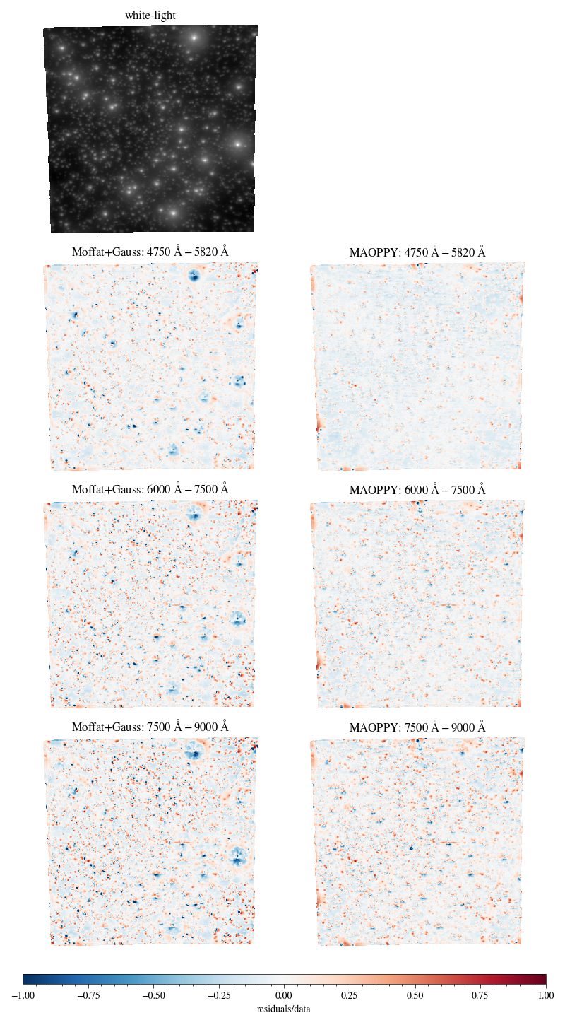
Figure 11: White-light image of a NFM observation and the residuals relative to the original data after subtracting the PSF model (left column: a combination of a Moffat curve with a Gaussian, right column: Maoppy) and background in three different wavelength ranges.

PampelMuse reconstructs the shape of the instrumental point spread function (PSF) in a datacube in order to extract spectra. While the PSF shape is the well known Moffat profile for MUSE WFM observations, it is more complicated in NFM observations. We implemented the PSF model Maoppy presented in Fétick et al. (2019) in PampelMuse to improve the source extraction. The model is designed for the situation typically faced in adaptive optics, where the PSF consists of a coherent core near the diffraction limit surrounded by a seeing-limited halo, the latter being the result of atmospheric turbulence with spatial frequencies uncorrected for by the deformable mirror. In the case of Maoppy, the diffraction-limited part of the PSF is adapted to the instrument in use, whereas the atmospheric residuals in the core are modelled as a Moffat function and the uncorrected spatial frequencies are modelled with the Kolmogorov turbulence model, which includes the Fried parameter $r_{0}$ to scale the turbulence strength. Figure 11 shows the residuals after PSF and sky subtraction relative to the original data in three different wavelength ranges for the Maoppy model and a combination of a Moffat profile with a Gaussian core. As the residuals shown in Fig. 11 slightly increase with increasing wavelength, we suspect that the atmospheric diffraction is not completely corrected. We will learn more about the peculiarities of NFM data after reducing more observations. The FWHM of the PSF in our observations decreases from 40 mas in the blue part of the spectrum to 30 mas in the red part. The Strehl ratio is about 5 per cent at 650 nm and increases to a maximum of 10 per cent at 900 nm.

We further noticed that the catalogue positions of a significant fraction of the resolved stars were not accurate enough at the high spatial resolution offered by the NFM. This became evident when we observed significant bipolar fit residuals around the centroids of the affected stars. Recall that by default, PampelMuse predicts the positions of the stars in the MUSE data via a global coordinate transformation from the reference catalogue. The origin of these inaccuracies could be physical (e.g., due to proper motions) or instrumental (e.g. caused by residual errors in the astrometric calibration performed by the data reduction pipeline). In order to account for these offset, a new feature was added to PampelMuse, which allows the user to determine individual offsets $\delta x$ and $\delta y$ for each star relative to the NFM positions predicted by the global coordinate transformation. In the case of M80, typical offsets of $0.4$ spatial pixels, corresponding to 10 mas, were applied. For comparison, a star with velocity of 10 $\text{km}\,\text{s}^{-1}$ in the plane of the sky at a distance of 10 kpc has moved about 3 mas since the HST observations in 2006 (Anderson et al., 2008). Further details on the improvements implemented in PampelMuse in order to deal with NFM data will be presented in a forthcoming paper.

3.2 Spectral analysis

To analyse the extracted spectra, we use our well-tested fitting pipeline described in Husser et al. (2016). Since the adaptive-optics correction works better in the red than in the blue part of the spectrum, the spectral noise is higher in the blue part. To take care of this systematic difference, the full-spectrum fit uses uncertainties derived from the variance extension of the datacube as weights for spectra extracted from NFM observations.

3.3 Improvements due to NFM observations

Compared to the previous study of M80 (Kamann et al., 2020), we obtain spectra of more than a thousand new stars in the central 7.5 arcsec by 7.5 arcsec from our NFM observations. Here, we only take into account stars with “useful” spectra which are spectra with a S/N above five, a radial velocity reliability of at least 90 per cent (see Section 3.4) and a MagAccuracy of more than 80 per cent (see definition in Kamann et al., 2018). We later use radial velocities resulting only from spectra that fulfil these criteria. Figure 2 shows a colour-magnitude diagram of stars inside the NFM region and indicates whether we have observed useful spectra with the WFM, the NFM, or if we did not get a useful spectrum. We analysed the spectra of 185 stars from the WFM observations of the cluster centre, 176 of them have spectra with a mean S/N of at least five, and 121 have a mean S/N of at least ten. With the NFM observations, we gain 932 stars that had no useful analysis result from previous observations. Of those 932 stars, 891 have spectra with a mean S/N of at least ten. The total number of stars with useful spectra inside the NFM footprint is 1072. This implies an overall completeness of 71 per cent compared to the combined photometric catalog of Anderson et al. (2008) and Dalessandro et al. (2018) which contains 1501 stars in the region covered by our NFM observations.

3.4 Filtering data for reliability and binarity

As described in Kamann et al. (2018), we estimate whether a star is a member of the cluster or a foreground star based on a model of the Galactic stellar population (Robin et al., 2003) in the direction of the cluster. Depending on its mean radial velocity and metallicity, each star is assigned a membership probability.

Regardless of whether a spectrum is extracted from a NFM or WFM observation, its radial velocity derived from the spectral fit is assigned a reliability. This reliability is defined in Giesers et al. (2019, Section 3.2) and it depends on the following properties: the S/N ratio of the respective spectrum, the quality of a cross-correlation with a suitable template model spectrum, the difference of the radial velocity derived from the cross-correlation and the full-spectrum fit, plausible uncertainties of the radial velocity from the cross-correlation and full-spectrum fit, and agreement between the fitted radial velocity and the mean cluster radial velocity. In this study, we include all radial velocities resulting from a fit with a reliability of more than 90 per cent.

When multiple radial velocities are available for a given star, we use the method described in Giesers et al. (2019) to compute the probability $p$ that they show temporal variability. Since the dynamical model we use is not able to take binary stars into account, we follow Kamann et al. (2020) and only include stars with $p<80$ per cent, removing 169 stars from further analysis (about 2 per cent of our final sample of stars). We average all reliable radial velocities of the same star weighted by their uncertainties to obtain a mean radial velocity. After filtering, we check the consistency of WMF and NFM observations by computing the mean radial velocity per star separately for WFM and NFM observations. For stars which were observed in both modes, the weighted mean difference of the WFM and NFM velocities is $-0.03\pm 0.77$ $\text{km}\,\text{s}^{-1}$. The number of stars in our analysis after filtering is 9720. In the further analysis, we use the measured radial velocities after subtracting the mean radial velocity of about 9.7 $\text{km}\,\text{s}^{-1}$.

This procedure removes two interesting stars very close to the Goldsbury et al. (2010) cluster centre (less than about 1 arcsec) with high radial velocities of $(88\pm 7)$ and $(101\pm 4)$ $\text{km}\,\text{s}^{-1}$ relative to the Solar System barycentre, respectively, and about 10 $\text{km}\,\text{s}^{-1}$ less relative to the cluster. It is plausible that both stars are cluster members and not foreground stars because of their low metallicities (both have $\text{[M/H]}\approx-2$) and their positions in the colour-magnitude diagram (on the main sequence and subgiant branch, see Fig. 2). We discuss these stars in Section 6.

3.5 External kinematic data

To increase the coverage of the outer parts of the cluster, we also include the radial velocities of Baumgardt & Hilker (2018). Stars that appear in both data sets have compatible velocities as shown by Kamann et al. (2020). Before combining these data with ours, we subtract the mean radial velocity from each individual velocity. Baumgardt & Hilker (2018) provide a probability P_single indicating whether a given star is a single star. We use this information to exclude stars with P_single less than 20 per cent and use the remaining 230 stars in our analysis. Their radial distances to the cluster centre are between 20 arcsec and 20 arcmin with a median of 3 arcmin. The total number of stars in our analysis is 9950. There are no proper motions available for the central regions of M80 because it is not part of the HST proper motion programme (Bellini et al., 2014).

4 Jeans model

4.1 Description

We use the axisymmetric Jeans model code cjam of Watkins et al. (2013) which is based on jam (Cappellari, 2008). cjam was also used in the previous analysis of Kamann et al. (2020). These Jeans models include the effects of anisotropy and rotation to calculate the first and second moments of the velocity distribution at a given point. We compared the model predictions to our data using the same maximum-likelihood approach as in Kamann et al. (2020). The advantage of this approach is that it does not bin the velocities but works with all individual data points. While this increases the computational complexity, it removes the subjective binning step from the analysis.

Since we share the basic model and analyse data of the same globular cluster, we adopt several parameters from the study of Kamann et al. (2020). In particular, we assume an axis ratio of $q=0.9$ for the cluster elongation. We also assume isotropy, i.e. the velocity dispersion along the line of sight and those tangential to it are identical ($\beta=0$). This assumption is justified by the core relaxation time of $10^{7.78}$ years (Harris, 1996) which suggests isotropy at the core radius (Watkins et al., 2015, Section 5.4).

Compared to the previous study, the model differs in the following aspects:

• The coordinates for the cluster centre are no longer fixed to the literature values. Instead, we use two new parameters, $\Delta x$ and $\Delta y$, with Gaussian priors centred on the photometric centre of Goldsbury et al. (2010) to account for uncertainties in the determination of the cluster centre.

• We compute a two-dimensional grid of 960 profiles in the form of Multi-Gaussian expansions that cover centre offsets between $-3$ arcsec and $+3$ arcsec relative to the Goldsbury et al. (2010) photometric centre and use the MGE of the closest grid point to compute the Jeans model during each MCMC step. To construct these profiles we used the HST photometry of Dalessandro et al. (2018) complemented by the Gaia data of de Boer et al. (2019) as described in Kamann et al. (2020), Section 4.1.

• As suggested by Hogg & Foreman-Mackey (2018), the rotation field is now parametrized by two vector components, $\kappa_{x}$ and $\kappa_{y}$, instead of its amplitude and an angle. While Kamann et al. (2020) determined the position angle before the main MCMC run, we vary these parameters together with all remaining ones during the MCMC run. As the Jeans code assumes the semi-major axis to be aligned with the x-axis of the coordinate system, we rotate our data by the current position angle estimate prior to calculating a new model.

• We include a potential for an IMBH parametrized by its mass. jam and cjam implement this by adding an additional Gaussian component to the MGE. At a mass of zero, the total potential is equal to the potential without a central IMBH. We take a uniform probability distribution between 0 and $15{,}000~{}\text{M}_{\odot}{}$ as a prior for the IMBH mass. We follow a comment in Cappellari (2008) and fix the standard deviation of the corresponding MGE component to $\sigma_{\text{PSF}}/3\approx 25$ mas.

For a given set of parameters, the Jeans code predicts the mean velocity and the velocity dispersion at the location of each star from our kinematic data set. As usual for MCMC approaches, we calculate parameter distributions by maximizing the product of the prior and the likelihood function, which is a Gaussian centered on the difference of measured velocities and the model prediction at that position (Watkins et al., 2013, Eq. 12). Table 2 lists the eleven parameters and their respective priors. We use the affine invariant ensemble MCMC sampler emcee (Foreman-Mackey et al., 2013). We use 192 walkers and a chain length of 2000 after burn-in.

4.2 Results

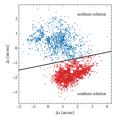
Figure 3: The distribution of centre offsets $\Delta x$ and $\Delta y$ is bimodal. We use the line $Y=0.2\Delta x-1\aas@@fstack{\prime\prime}{}1$ to separate the samples into a northern solution with $\Delta y>Y$ and a southern solution with $\Delta y<Y.$

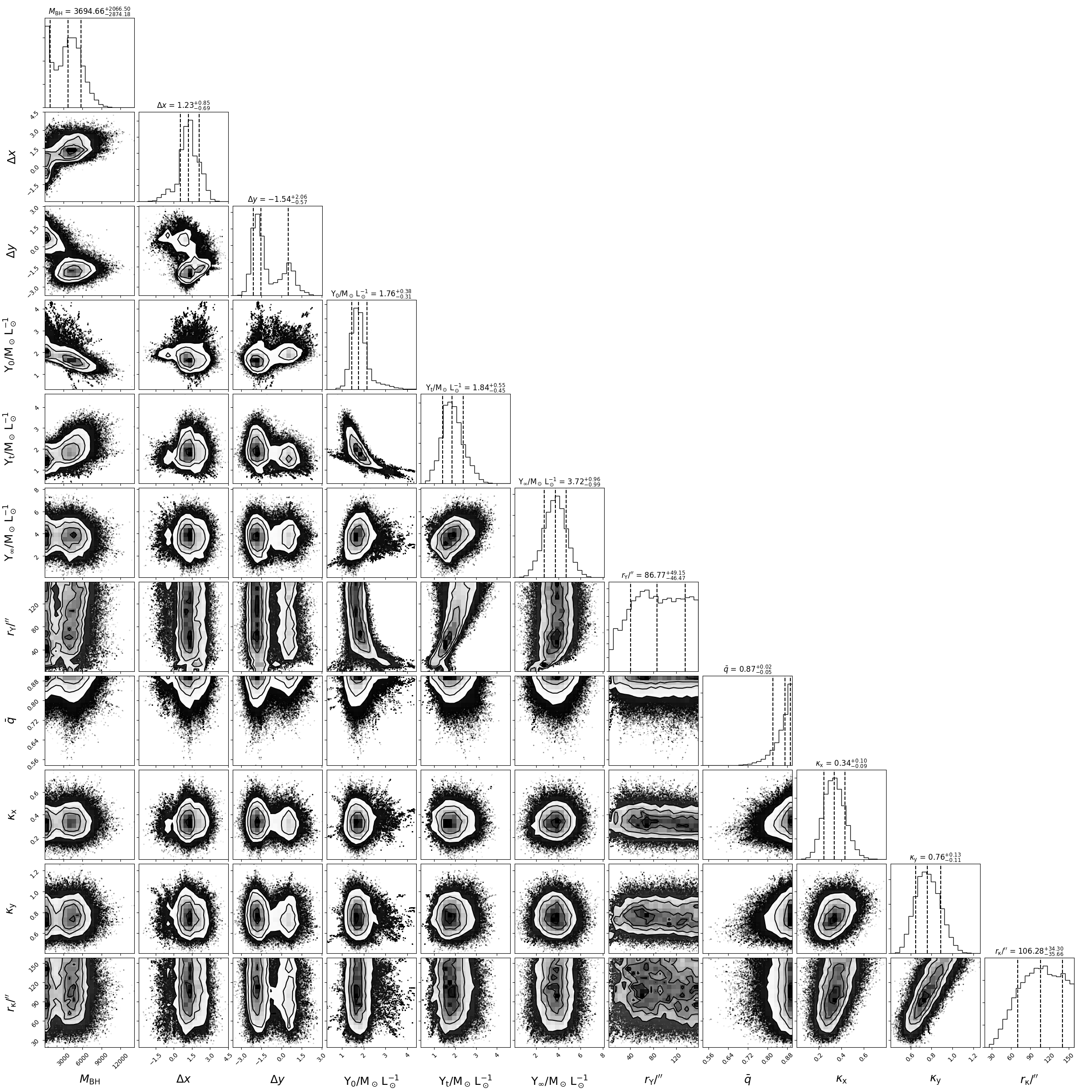
Figure 12: Corner plot of our final MCMC chain. See Table 2 for a description of the parameters.

The parameter distributions that we generate with the MCMC sampler (see Fig. 12) are bimodal in the centre offsets $\Delta x$ and $\Delta y$. As shown in Fig. 3, we separate the samples along the line $Y=0.2\Delta x-1\aas@@fstack{\prime\prime}{}1$ in the $\Delta x\Delta y$-plane. About one third of all samples have $\Delta y\geq Y$ and we name them ‘northern solution’, we name the other two thirds with $\Delta y<Y$ ‘southern solution’. The four circular gaps visible in the southern solution are each centered on a grid point of the MGE grid. The MGE at these locations have one component fewer than the surrounding ones and while they fit the surface brightness profile, they apparently cause a decrease in the likelihood when used as input for the Jeans model to fit the velocities. We present the overall parameter distribution resulting from the MCMC sampling in this section when there is no difference between the northern and the southern solutions and comment on the difference if there is any.

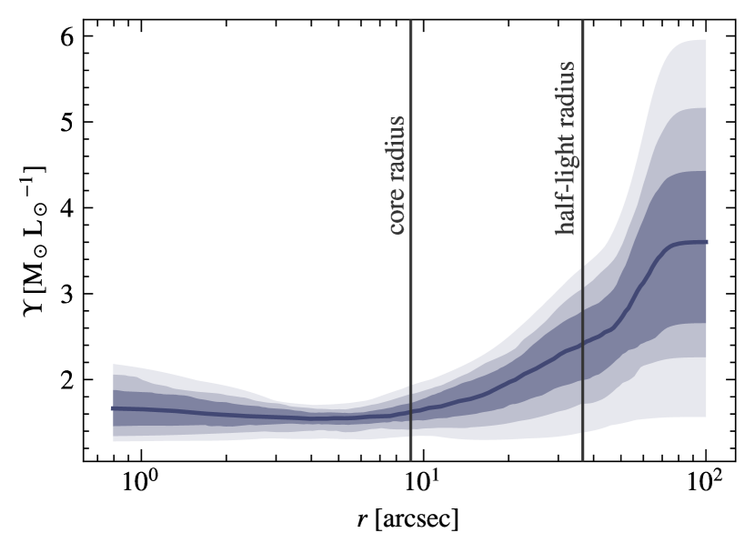
Figure 13: Radial profiles of the mass-to-light ratio $\Upsilon$, the blue lines corresponds to the median, the shaded areas are the $1\sigma$, $2\sigma$, and $3\sigma$ limits.

The profile of the mass-to-light ratio $\Upsilon(r)$ has a minimum at $r_{\Upsilon}=1.4^{+0.9}_{-0.8}\arcmin{}.$ We find a mean value of $\Upsilon=1.87\pm 0.15\,\text{M}_{\odot}\,\text{L}_{\odot}{}^{-1}$ for the cluster which is consistent with the value of $\Upsilon=1.72\pm 0.20\,\text{M}_{\odot}\,\text{L}_{\odot}{}^{-1}$ determined in Kamann et al. (2020) and also with $\Upsilon=1.93\pm 0.12\,\text{M}_{\odot}\,\text{L}_{\odot}{}^{-1}$ from Baumgardt et al. (2020). We plot profiles of the mass-to-light ratio $\Upsilon(r)$ using random samples drawn from our chain in Fig. 13. The total cluster mass is $(3.0_{-0.3}^{+0.2})\times 10^{5}~{}\text{M}_{\odot}{}.$

For the median intrinsic flattening we find $\bar{q}=0.86^{+0.03}_{-0.05}$ which is also consistent with $\bar{q}=0.83\pm 0.06$ found by Kamann et al. (2020). This corresponds to an inclination of $60\degr{}\pm 15\degr{}.$

The histograms of all eleven free parameters of the fitted Jeans model and their pairwise correlations are shown in Figure 12.

4.2.1 Dispersion and rotation profiles

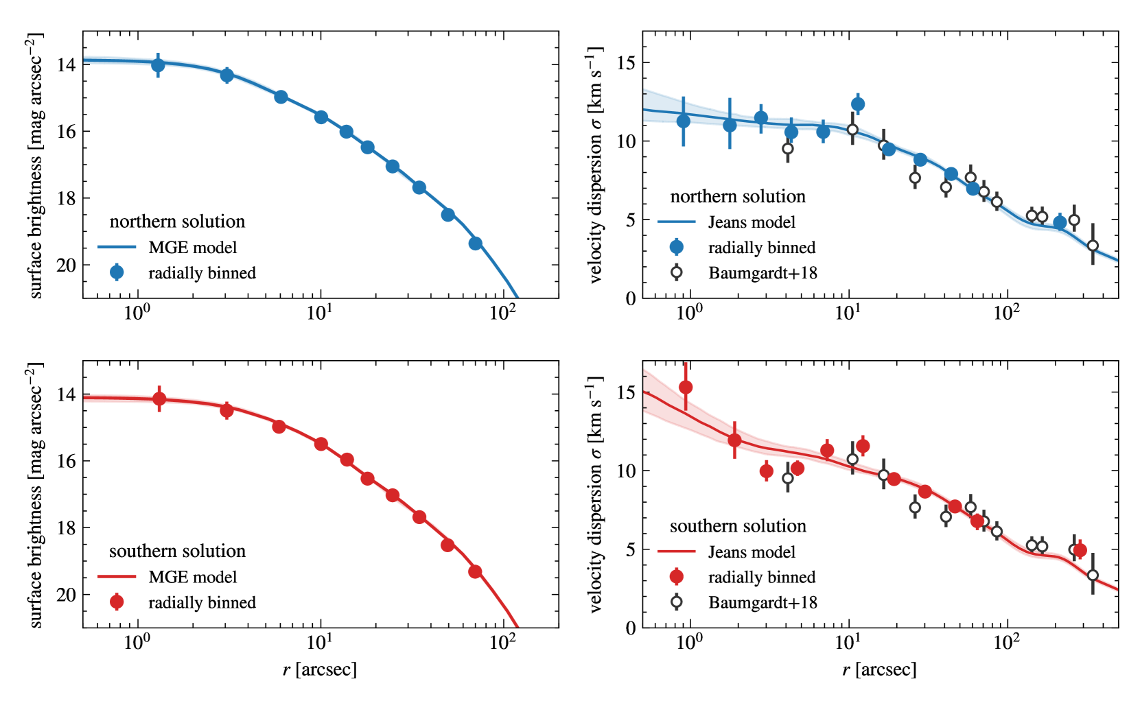
Figure 4: Radial profiles of the surface brightness (left column) and the velocity dispersion (right column). In the left column, filled circles show the profile derived using the photometry presented in Dalessandro et al. (2018), while the solid line shows our best-fit MGE model. In the right column, filled circles indicate the dispersion obtained directly from the MUSE data, whereas solid lines indicate the predictions from the Jeans models. In all panels, errorbars and shaded areas represent the 14th and 86th percentiles. The top row includes only MCMC samples from the northern solution, the bottom row only from the southern solution. The reference data from Baumgardt & Hilker (2018) is plotted as published, i.e. without taking into account any centre offset.

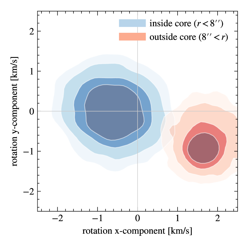
Figure 5: Joint distribution of the estimated x- and y-component of the rotation velocity. Each set of contours contains 50, 68, 87, and 95 per cent of all samples (from inner- to outermost) belonging to the core region (blue) or the outer region (red) of M80. The outer region is rotating, but it is not clear if the cluster core ($r<8$ arcsec) is also rotating.

To compare if the complex kinematic model actually reproduces our data, we plot the velocity dispersion profiles computed from the parameters in the chain with our data in Fig. 4. This figure also shows a comparison of the observed surface brightness profile and the fitted MGE models.

We binned the data radially and applied a much simpler kinematic model to each bin which determines a constant velocity dispersion and the components $v_{x}$ and $v_{y}$ of the rotational vector. In this model, the predicted radial velocity follows a Gaussian probability distribution with dispersion $\sigma$ and a mean that depends on the model parameters $v_{\text{sys}}$, $v_{x}$, and $v_{y}$ and on the position angle $\theta$ of a star according to

$$v(\theta)=v_{\text{sys}}+\sqrt{v_{x}^{2}+v_{y}^{2}}\,\sin[\theta-\arctan(v_{x}/v_{y})],$$ (1)

where $\theta-\arctan(v_{x}/v_{y})$ is the angular distance to the rotation axis. To account for the uncertainty of the cluster centre coordinates, we repeat the binning for 250 potential centres drawn from the MCMC chain. The values from this simple model and the Jeans model agree with each other. Furthermore, Fig. 4 shows the velocity dispersions used in the analysis of M80 by Baumgardt & Hilker (2018) which also agree with our values. The Jeans model has a central velocity dispersion (at radius of 1 arcsec) of $12.8\pm 1.3$ $\text{km}\,\text{s}^{-1}$, which is about 2 $\text{km}\,\text{s}^{-1}$ more than the value of $10.5\pm 0.5$ $\text{km}\,\text{s}^{-1}$ from Baumgardt & Hilker (2018). The northern solution has a lower central velocity dispersion of $11.7\pm 0.6$ $\text{km}\,\text{s}^{-1}$ and the southern solution has a central velocity dispersion of $13.4\pm 0.8$ $\text{km}\,\text{s}^{-1}$. To check if the higher values for the central velocity dispersion of the southern solution is an artefact caused by a few stars with unusual radial velocities, we plotted the radial velocity of individual stars close to the respective centres as a function of the centre distance. We did not find any outliers in these plots. Instead, the overall scatter in the radial velocities is larger around the centre of the southern solution. To further check how reliable the increased velocity dispersion around the southern centre is, we compute the biweight scale of the radial velocities, a robust measure of the standard deviation (see Beers et al., 1990) for the $n$ nearest neighbours of each star in the NFM field of view ($n=20,40,100$). This method also shows an increase in the velocity dispersion around the southern centre but not around the northern one.

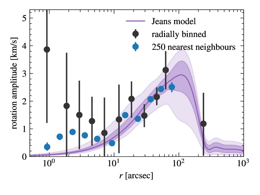
Figure 14: Radial profile of the rotation amplitude derived from the Jeans model, from individual radial velocities in radial bins, and from the mean radial velocities of the 250 nearest neighbours of each star.

We find an overall rotation angle of $66\degr{}\pm 6\degr{}$, consistent with the angle of $60\degr{}\pm 3\degr{}$ found by Kamann et al. (2020). Figure 14 shows the radial profile of the rotation amplitude derived from the final MCMC chain. That figure also shows the rotation amplitude computed using the same radial bins and model as for the dispersion plot described above. The radial rotation profile follows the one from Kamann et al. (2020) as expected. The binned data show a very large uncertainty towards the cluster centre because the bin radii are similar to the uncertainty in the centre coordinates.

As a consistency check, we also compute the biweight location of the radial velocities, a robust measure for the mean (Beers et al., 1990), for $n=250$ nearest neighbours of each star in the central $100\arcsec{}\times 100\arcsec{}$. We calculate the rotational parameters from these velocities by treating them as ordinary velocities in our simple model (Eq. 1). As demonstrated in Fig. 14, the rotational amplitude and angle derived in this way have a similar radial profile as the ones directly computed from the radial velocities.

Figure 6: Contour plot of our estimate of the kinematic centre of M80. The blue-shaded regions cumulatively contain 68, 87, and 95 per cent of all samples (from inner- to outermost). The two white crosses are the centres of the northern and the southern solution. G10 denotes the centre found in Goldsbury et al. (2010), L13 is from Lützgendorf et al. (2013), and D18 is the centre of Dalessandro et al. (2018). The smaller circles mark the potential central high-velocity main-sequence (HV-MS) and subgiant (HV-SG) stars. The orange line indicates the rotation axis of the whole cluster and its uncertainty computed from the 16th and 84th percentiles, using G10 as the reference centre.

We had a closer look at whether the core of M80 rotates. While such a central rotation component is expected to be short-lived because of the effects of two-body relaxation, evidence for a decoupled core has for example been reported in the core collapse cluster NGC 7078 (van den Bosch et al., 2006; Usher et al., 2021). The central rotation curve strongly depends on the position of the cluster centre since we use the radial distance to the centre for binning. To account for the uncertainty in the position of the cluster centre, we draw 250 pairs of the centre position offsets $\Delta x$ and $\Delta y$ from our final MCMC chain. Figure 5 shows the joint distribution of the x- and y-component of the rotation velocity for different radial bins. While we find a clear rotation signal of $v_{\text{rot}}=1.9\pm 0.4$ $\text{km}\,\text{s}^{-1}$ in the outer parts of the cluster, similar to the value of $1.97\pm 0.84$ $\text{km}\,\text{s}^{-1}$ determined by Sollima et al. (2019, Table 1), it is less clear if the cluster core ($r_{\text{core}}\approx 8\arcsec{},$ Harris, 1996; Baumgardt & Hilker, 2018) is rotating. In this region, the rotation components follow a broad distribution with a median of 0.9 $\text{km}\,\text{s}^{-1}$, 90 per cent of all samples are below $v_{\text{rot}}=1.6$ $\text{km}\,\text{s}^{-1}$. We note that the central rotation angle is offset from the rotation angle in the outer parts of the cluster by about $150\degr{}\pm 30$°.

4.2.2 Position of the cluster centre

The centres of globular clusters are usually determined using photometric data. There are three recent measurements for the cluster centre of M80. Goldsbury et al. (2010) found $\text{RA}=16\text{h}\,17\text{m}\,2.41\text{s}$ and $\text{Dec}=-22\degr{}58\arcmin{}33\aas@@fstack{\prime\prime}{}9$ with an uncertainty of $0\aas@@fstack{\prime\prime}{}2$, while Dalessandro et al. (2018) found $\text{RA}=16\text{h}\,17\text{m}\,2.481\text{s}$ and $\text{Dec}=-22\degr{}58\arcmin{}34\aas@@fstack{\prime\prime}{}098$ with an uncertainty of $0\aas@@fstack{\prime\prime}{}17$, and Lützgendorf et al. (2013) found $\text{RA}=16\text{h}\,17\text{m}\,2.4\text{s}$ and $\text{Dec}=-22\degr{}58\arcmin{}32\aas@@fstack{\prime\prime}{}6$ with an uncertainty of $0\aas@@fstack{\prime\prime}{}7$. We compare these centres with the offsets in the centre position as sampled by our MCMC chain by transforming the offsets to equatorial coordinates and plotting their density in Figure 6. The centre of the northern solution is located at

$$\text{RA}=16\text{h}\,17\text{m}\,2.36\text{s},~{}\text{Dec}=-22\degr{}58\arcmin{}33\aas@@fstack{\prime\prime}{}4,$$ (2)

and the centre of the southern solution is located at

$$\text{RA}=16\text{h}\,17\text{m}\,2.30\text{s},~{}\text{Dec}=-22\degr{}58\arcmin{}35\aas@@fstack{\prime\prime}{}7.$$ (3)

As these centres are determined from a dynamical model and to distinguish it from the photometric centres, we call them dynamical centres. The contours around the dynamical centres in Fig. 6 show the uncertainties which are larger than those for the photometric centres. While the centre of the northern solution is close to the known photometric centres, especially to the ones from Goldsbury et al. (2010) and Lützgendorf et al. (2013), the southern centre is located at a distance of about 2.4 arcsec to the south-west of the northern centre.

4.2.3 Limits on the IMBH mass

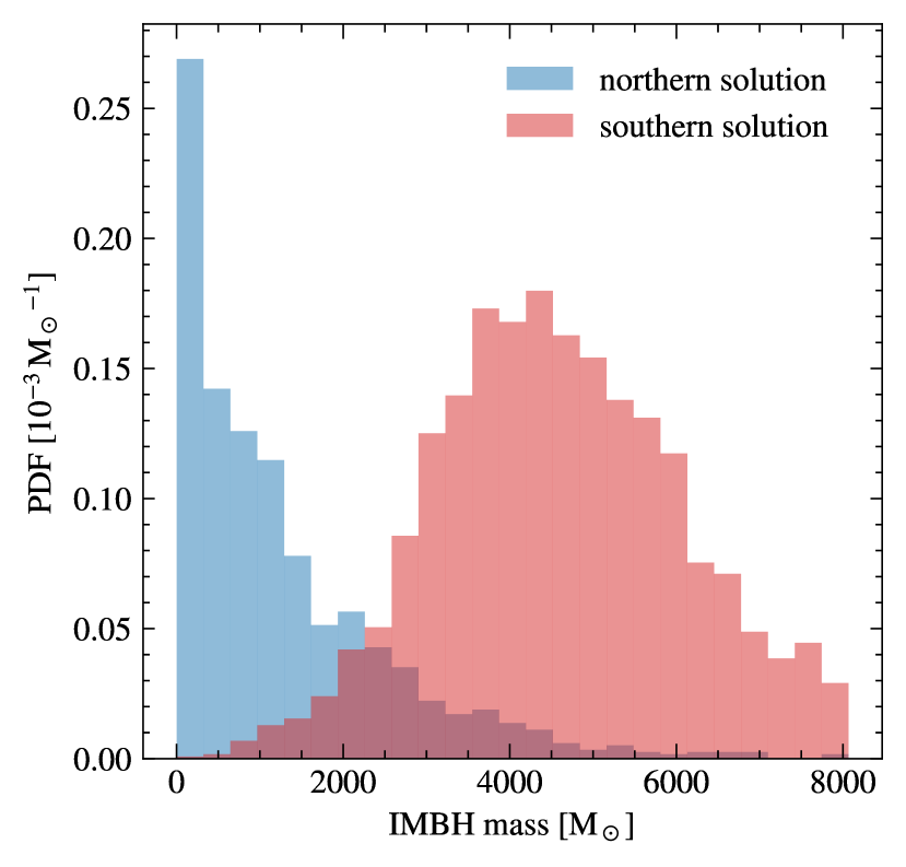
Figure 7: Distribution of the IMBH masses obtained via Jeans modelling around different centres.

The posterior distribution of the mass has a peak at masses below $1000~{}\text{M}_{\odot}{}$ and another peak at about $5000~{}\text{M}_{\odot}{}$. The uncertain position of the centre has a large impact on the shape and moments of the distribution of the IMBH mass, as can be seen from Fig. 7. Here, we compare the IMBH mass distributions of the northern and the southern solutions. The 90-per-cent upper limits on the IMBH mass (rounded to the nearest $100~{}\text{M}_{\odot}{}$) are $3000~{}\text{M}_{\odot}{}$ and $6800~{}\text{M}_{\odot}{}$, respectively. Given a peaked shape of the IMBH mass distributions for the southern centre, we also report a median IMBH mass and an $1\sigma$ uncertainty of $4600^{+1700}_{-1400}~{}\text{M}_{\odot}{}$ around this centre.

5 N-body models

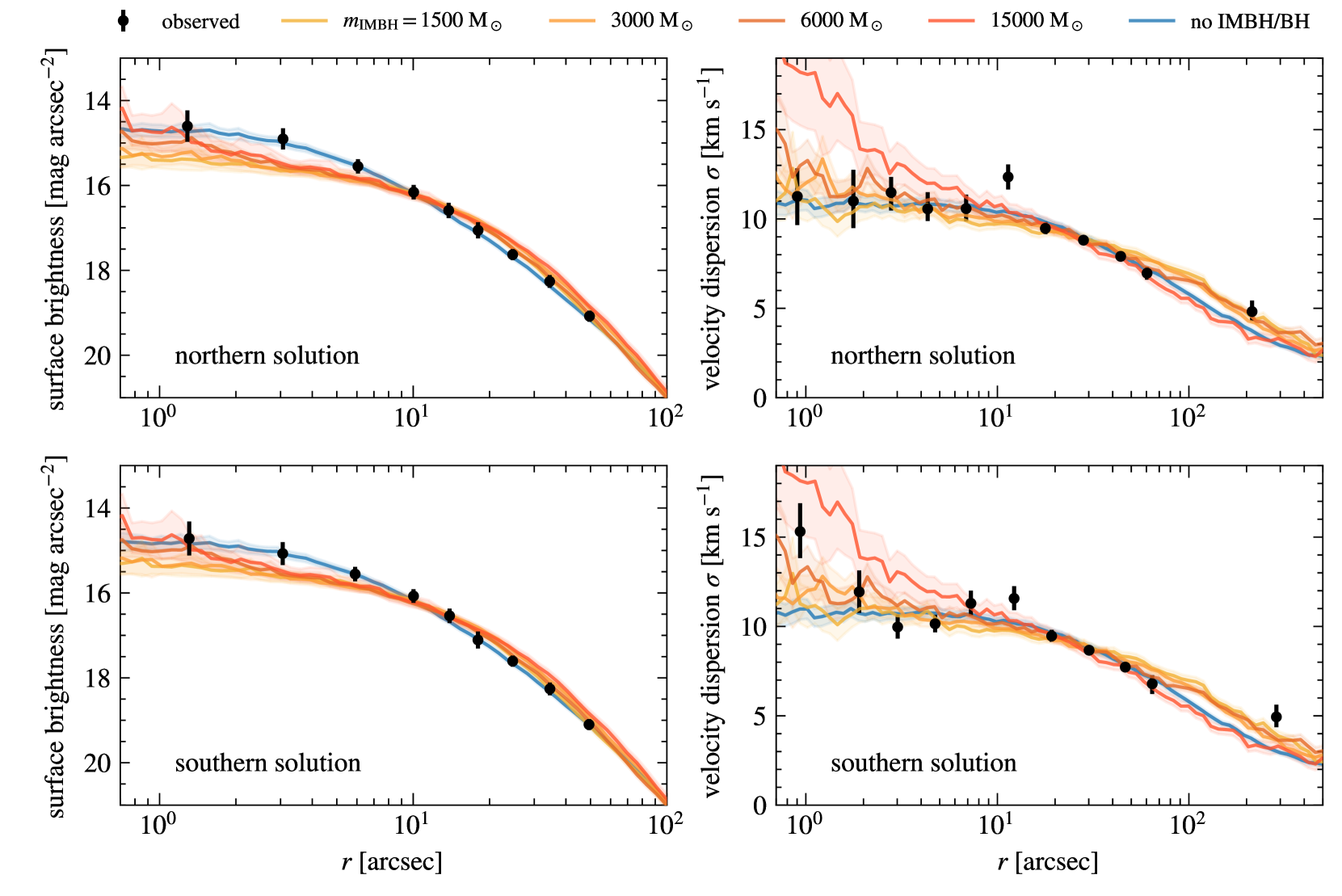
Figure 8: Comparison of the observed surface brightness and the observed velocity dispersion computed from radial bins around the northern and southern centre, respectively, to $N$-body models with an IMBH. See Tables 3 and 4 for more details on the models.

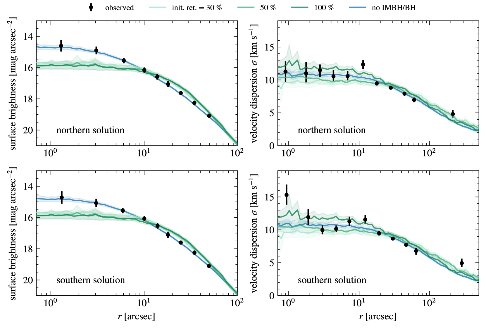
Figure 9: Comparison of the observed surface brightness and the observed velocity dispersion computed from radial bins around the northern and southern centre, respectively, to $N$-body models with stellar-mass BHs. The $N$-body models have different initial retention fractions for stellar-mass BHs, see Tables 3 and 4 for more details on the models.

In order to further investigate if the observed velocity dispersion of M80 requires the presence of an IMBH, we fit a grid of $N$-body models against the observed surface brightness and velocity dispersion profiles. In particular we use the grid of IMBH models presented by Baumgardt (2017) and the grid of models with varying stellar-mass back hole retention fractions presented in Baumgardt et al. (2019). Baumgardt (2017) and Baumgardt et al. (2019) have run a grid of about 3000 $N$-body simulations of star clusters containing $N=100{,}000$ or $N=200{,}000$ stars using nbody6 (Aarseth, 1999; Nitadori & Aarseth, 2012), varying the initial density profile and half-mass radius, the initial mass function and the mass fraction of an intermediate mass black hole in the clusters. Figure 8 compares the best-fitting models without an IMBH and with IMBHs containing 0.5, 1.0, 2.0 and 5.0 per cent of the final cluster mass of $3\times 10^{5}~{}\text{M}_{\odot}{}$ with the observed velocity dispersion profile and the observed surface brightness profile for the northern and southern centre solutions (also see Tables 3 and 4). Around the southern centre it can be seen that models with an IMBH lead to somewhat better fits of the velocity dispersion profile, whereas the surface brightness profile is better reproduced by the models without an IMBH. Measuring the error weighted difference between observed and predicted velocity dispersion and dividing by the number of degrees of freedom, we obtain a reduced $\chi^{2}_{r}$ value of 1.54 for the 2-per-cent IMBH model from the fit to the velocity dispersion profile, while a no-IMBH solution gives $\chi^{2}_{r}=2.25$. Including the fit to the surface brightness profile as well, the reduced $\chi^{2}_{r}$ value is 1.16 for the 2-per-cent IMBH model and 1.51 for the 0.5-per-cent IMBH model while the no-IMBH model has $\chi^{2}_{r}=1.24$. Hence the $N$-body models confirm the results of the Jeans modelling that an IMBH of a mass of around 6000 $\text{M}_{\odot}{}$ provides an acceptable fit for M80 if the southern solution is adopted as the density centre. A no-IMBH model does however provide a good fit around this centre as well. Around the northern centre we find similar fit results. The no-IMBH solution provides the best fit but the IMBH models result only in slightly worse fits and are also acceptable solutions. Again, the surface brightness profile is better reproduced by a model without any IMBH. Thus, if the northern centre is adopted, an IMBH with a mass of up to about 6000 $\text{M}_{\odot}{}$ is possible as well.

The corresponding fit of models with different retention fractions of stellar-mass black holes is depicted in Fig. 9. We obtain rather poor fits to the surface brightness profile for models with retention fractions of stellar mass black holes greater than 30 per cent. The fits become worse the larger the assumed retention fraction of stellar-mass black holes. This is particularly striking for the surface brightness profile, as all models with significant retention fractions produce a core that is larger than what is observed, in agreement with the prediction that clusters harbouring a considerable number of black holes should have large core radii (Arca Sedda et al., 2018). We therefore conclude that the initial retention fraction of black holes in M80 was low or that nearly all stellar-mass black holes have been ejected from this cluster.

6 Discovery of two stars with high radial velocity

We find two stars very close to the Goldsbury et al. (2010) cluster centre (with a distance less than about 1 arcsec, see Fig. 6) with a high radial velocity relative to the Solar System barycentre: a main-sequence star with $v=(88\pm 7)$ $\text{km}\,\text{s}^{-1}$ at a projected distance of 1.1 arcsec ($\text{RA}=16\text{h}\,17\text{m}\,2.345\text{s}$, $\text{Dec}=-22\degr{}58\arcmin{}33\aas@@fstack{\prime\prime}{}33$) and a subgiant star with $v=(101\pm 4)$ $\text{km}\,\text{s}^{-1}$ at a projected distance of 0.4 arcsec ($\text{RA}=16\text{h}\,17\text{m}\,2.414\text{s}$, $\text{Dec}=-22\degr{}58\arcmin{}33\aas@@fstack{\prime\prime}{}51$). While we have two spectra of the main-sequence star and three spectra of the subgiant, we could only derive one and two useful radial velocities respectively due to the low signal-to-noise of the remaining spectra. The radial velocity of both stars is well above the central escape velocity of M80 (41.4 $\text{km}\,\text{s}^{-1}$, Baumgardt & Hilker, 2018).

High-velocity stars have been reported in three other clusters: in NGC 2808 (Lützgendorf et al., 2012), in M3 (Gunn & Griffin, 1979), and in 47 Tuc (Meylan et al., 1991). In these cases, two stars were detected with a radial velocity a few times the velocity dispersion above or below the mean cluster velocity but below the central escape velocity of the respective cluster.

The high radial velocity of these two stars can be explained in several ways:

Foreground star

One or both stars could be foreground stars instead of cluster members. Using the Besançon model (Robin et al., 2003) of the region close to M80, we estimate that about 0.7 per cent of all foreground stars have $-2.25<\text{[Fe/H]}<-1.75$, $|v|>80$ $\text{km}\,\text{s}^{-1}$ and a V brightness above 21 mag. As we find $n=25$ non-member stars in the central 6 arcsec, the probability of having one high-velocity non-member star in this region is 16 per cent, and it is 5 per cent for the central 1.5 arcsec. The probability that two or more such stars are present is about 1 per cent and 0.04 per cent, respectively. In order to further investigate the membership of the fast-moving stars, we analysed two sets of HST observations, one obtained in 2006 (HST proposal ID 10775, PI Sarajedini) and one taken in 2012 (HST proposal ID 12605, PI Piotto). We analysed each data set using Dolphot (Dolphin, 2000, 2016) and transformed the HST coordinates into the ICRS reference frame by cross-matching the stellar coordinates against those of the Gaia EDR3 catalogue (Gaia Collaboration et al., 2021). For each data set, we performed an epoch transformation of the Gaia coordinates back to the epoch when the HST observations were taken, using the measured Gaia proper motions of the stars. Comparison of two sets of stellar coordinates obtained from the cross-matching then allows us to calculate the absolute proper motions of the stars. We obtain a mean cluster motion of ($\mu_{\alpha}*,\mu_{\delta}$) = ($-3.03\pm 0.05,-5.61\pm 0.05$) mas yr^-1, in good agreement with the proper motion found by Vasiliev & Baumgardt (2021) from the Gaia EDR3 data directly. For the fast-moving SGB star we find a mean proper motion of of ($\mu_{\alpha}*,\mu_{\delta}$) = ($-3.37\pm 0.45,-5.87\pm 0.45$) mas yr^-1, well within the range of proper motions that we obtain for the other member stars and fully compatible with a cluster membership of this star. We therefore consider it likely that the SGB star is a cluster member. Unfortunately we are not able to determine a proper motion for the main-sequence star.

Binary star

The orbital motion of stars in a binary system could be the source for the high radial velocity. Since we only have two radial velocities ($104.9\pm 6.4$ and $99.1\pm 5.4$ $\text{km}\,\text{s}^{-1}$) taken about 10 months apart for the subgiant star and only one for the main-sequence star, we cannot entirely exclude variations in the radial velocity. However, we note that our measurements are consistent with a constant radial velocity. Plausible binary system configurations that would produce a velocity amplitude of about 90 $\text{km}\,\text{s}^{-1}$ containing a star with a mass of $0.75~{}\text{M}_{\odot}{}$ are a short-period system with a low-mass star, a system with a compact host (white dwarf, neutron star, stellar-mass black hole) with a period of several days, or a system with an IMBH as host with a period of several years. To estimate the number of suitable binary systems, we use a binary fraction of 5 per cent estimated from our data, comparable to the low binary fraction of less then about 5 per cent in this cluster (see Milone et al., 2012; Ji & Bregman, 2015). This value is higher than the 2 per cent of stars removed from our sample because of radial velocity variations (Section 3.4) since it is corrected for incompleteness due to a limited number of epochs and low velocity variations. Assuming that 1 per cent of all binary systems have a suitable configuration, we expect 0.5 of 1000 stars to be in such stellar binary systems. If one of the stars is in a bound orbit around an IMBH with a mass of $4000~{}\text{M}_{\odot}{}$, its orbital distance must be less than $2m_{\text{IMBH}}G/v^{2}$ which corresponds to 0.1 arcsec at the distance of M80. This also excludes the possibility that both stars are bound to the same IMBH.

Radial velocity outlier

Since the radial velocities of both stars are about 40 and 50 $\text{km}\,\text{s}^{-1}$ greater than the cluster escape velocity of 41.4 $\text{km}\,\text{s}^{-1}$ (Baumgardt & Hilker, 2018), the stars are not gravitationally bound to the cluster.

Accelerated by interaction

Interactions between binary systems with a single stellar-mass black hole can scatter one of the stars in the binary system and accelerate it to high velocities (e.g. Lützgendorf et al., 2012). We expect the probability of this process to be proportional to the number of stellar-mass black holes in the cluster, which is low according to the best-fitting N-body models. Similarly, an IMBH, if present, should be able to scatter stars in the same way as a stellar-mass black hole.

In conclusion, the mechanism leading to the high radial velocities is not obvious. One of the most likely explanations, the Kepler motion in a binary system, could easily be confirmed or rejected with a few additional measurements.

7 Discussion

Our MCMC sampling reveals the existence of two possible solutions for the centre offsets of the Jeans model of M80: the northern solution has the centre close to the photometric centres from the literature and it does not need an IMBH to describe the observed kinematics, and a southern solution with a centre at a distance of about 2.4 arcsec from the northern one that needs an IMBH with a mass of $4600^{+1700}_{-1400}~{}\text{M}_{\odot}{}.$

The dynamical centre of the southern solution is at a distance of about 2 to 3 arcsec from the photometric centres in the literature. A distinct dynamical centre would indicate a perturbed system, possibly caused by an IMBH. We note that a distinct dynamical centre would be inconsistent with the assumption that the cluster can be described with a Jeans model where photometric and dynamical centre are the same by construction. We try to minimize this discrepancy by choosing an MGE profile constructed for the current centre in each iteration. Physically, the position of the IMBH is not expected to be identical with the photometric or dynamical centre. $N$-body models predict that the IMBH will wander inside a sphere with a characteristic radius, the wandering radius $r_{w}$, around the centre. de Vita et al. (2018) analysed $N$-body models and found a scaling relation for this radius which depends on a number of cluster parameters (de Vita et al., 2018, Eq. 17). Using values for the core density and radius from Baumgardt & Hilker (2018) and assuming a mean stellar mass in the core of $0.65~{}\text{M}_{\odot}{}$, we find $r_{w}\approx 0\aas@@fstack{\prime\prime}{}4$ for an IMBH mass of about 3000 to $4600~{}\text{M}_{\odot}{}$. This radius is less than the distance between photometric and dynamical centre of the southern solution, indicating that the wandering motion can not be the explanation for the observed offset. The sphere of influence of an IMBH with a mass of 4600 $\text{M}_{\odot}{}$ has a radius of 0.09 pc (Peebles, 1972), corresponding to 1.8 arcsec at the distance of M80.

Lützgendorf et al. (2013) found a $1\sigma$ upper limit of $800~{}\text{M}_{\odot}{}$ for an IMBH in M80 using data from the integral-field spectrograph FLAMES/ARGUS. This value is well below all upper limits we derived. Lützgendorf et al. (2013) calculated their own position of the cluster centre (see Fig. 6) and did not obtain the velocity dispersion by analysing spectra of individual stars, instead they combined unresolved spectra in radial bins. Their velocity dispersion profile is systematically lower in the cluster centre than ours: while our profile (Fig. 4) is above 10 $\text{km}\,\text{s}^{-1}$ for all radii below 10 arcsec (even after accounting for the uncertainty in the determination of the correct centre), their profile stays below 10 $\text{km}\,\text{s}^{-1}$. As discussed by Bianchini et al. (2015), there are possible systematic errors in both methods, integrated-light spectroscopy and single-star kinematics. However, a common criticism regarding the latter is that the dispersion would be biased towards low values because of contamination from unresolved stars. The fact that our dispersion measurements are above those by Lützgendorf et al. (2013) suggests that our method is not affected by this. Our IMBH mass upper limit of $3000~{}\text{M}_{\odot}{}$ for the northern solution is below the IMBH mass estimate of $(3.63\pm 0.95)\times 10^{3}\,\text{M}_{\odot}{}$ predicted from Monte-Carlo models (Arca Sedda et al., 2019), while the median IMBH mass of the southern solution agrees with their result. Estimates for the mass of an IMBH in M80 based on the $M_{\bullet}$-$\sigma$ correlation and similar correlations range from 1000 to 2610 $\text{M}_{\odot}{}$ (Safonova & Shastri, 2010, Table 6).

We assumed that the cluster kinematics can be described by an isotropic model (see Section 4.1). As Zocchi et al. (2017) point out, radially anisotropic models of NGC 5139 show an increase in the central velocity dispersion similar to that due to the influence of an IMBH. If our assumption about isotropy is not satisfied in M80, our isotropic model would overestimate the IMBH mass. Since the cluster has a ratio of age to relaxation time greater than ten, the $N$-body models used in Lützgendorf et al. (2011) imply that the cluster centre is isotropic.

The comparison to $N$-body models performed in Section 5 suggests that the observed steep surface brightness profile of the cluster is better explained by models without IMBH. The binned surface brightness profile presented in Figures 4, 8 and 9 is derived from the photometry of Dalessandro et al. (2018) which is based on HST observations. This profile is about 0.5 to 0.8 mag arcsec^-2 brighter in the central bins compared to the profile of Noyola & Gebhardt (2006) and about 1 to 1.3 mag arcsec^-2 brighter than the profiles of Trager et al. (1995) computed from ground-based photometry. Figures 8 and 9 indicate that the other surface brightness profiles with lower central values is less well fitted by the no-IMBH model and better fitted by the models with an IMBH. An important difference between the two aforementioned surface brightness profiles and the one derived in this work is that the former are based on actual brightness measurements, whereas we adopted star counts. Profiles based on star counts are robust against shot noise effects caused by individual bright stars, yet require complete photometry even in the crowded cluster centres. The availability of ACS-HRC data makes us confident that our results are not affected by incompleteness. Note that we only included stars brighter than F435W $<19.6$ mag, i.e. about the main-sequence turn-off, when determining the number density profiles.

Ultimately, our models cannot answer the question which of the two solutions for the cluster centre is to be preferred, and therefore whether an IMBH exists in M80. In light of the better agreement with the photometric determinations of the cluster centre, the northern solution seems the more likely one. However, our models do include a prior which favours solutions in agreement with the photometric centres. Hence, in case the true cluster centre coincides with the photometric estimates (and our northern solution), the high velocity dispersion around the centre of the southern solution is leading our Jeans models astray. As mentioned earlier, we verified that no individual high-velocity stars are responsible for the occurrence of the southern solution. Still, we cannot exclude that some of our model assumptions, such as a Gaussian line-of-sight velocity distribution or axisymmetry, are violated by the actual kinematics in the centre of M80.

8 Conclusions

We used spectra obtained with state-of-the-art adaptive optics of the central region in M80 to analyse kinematic properties of the cluster. We built on an axisymmetric Jeans model used previously for this cluster by Kamann et al. (2020) and introduced additional parameters to describe a hypothetical intermediate-mass black hole and offsets between the photometric centre and the kinematic centre. The parameter samples of our Jeans model show a bimodal distribution in the centre offsets: a third of all samples are part of a northern solution with a centre close to the known photometric centres, the other two thirds are part of the southern solution with a centre at a distance of about 2.4 arcsec from the northern centre. While most parameters do not show significant differences between the two solutions, the distribution of mass of the central IMBH is different. Around the northern centre, we find a distribution with a peak below $1000~{}\text{M}_{\odot}{}$ that quickly decreases with increasing IMBH mass. The 90-per-cent upper limit is $3000~{}\text{M}_{\odot}{}.$ The IMBH mass distribution of the southern solution has a median and an $1\sigma$ uncertainty of $4600^{+1700}_{-1400}~{}\text{M}_{\odot}{}$, 90 per cent of all samples are below $6800~{}\text{M}_{\odot}{}.$ $N$-body models support the existence of an IMBH in this cluster with a mass of up to $6000~{}\text{M}_{\odot}{}$ although models without an IMBH provide a better fit to the observed surface brightness profile. They further indicate that the cluster has lost nearly all stellar-mass black holes. The overall radial profiles of the mass-to-light-ratio and the rotation velocity agree with the previous analysis of this cluster (Kamann et al., 2020). While the part outside the cluster core clearly rotates, it is not clear whether the core of the cluster is rotating. Our analysis is consistent with no rotation in the centre but the uncertainty in the position of the cluster centre prohibits any definitive conclusion. We discussed the detection of two central stars with radial velocities clearly above the escape velocity of the cluster. Their high velocities could be explained if one or both stars belong to the Milky Way population instead to M80, if they are caused by binary motion, or if one or both stars were accelerated by interactions between a binary system and a stellar-mass or intermediate-mass black hole. Of these possibilities, the periodic change of radial velocity due to binary motion can be confirmed or ruled out by future observations.

Proper-motion data of stars in the cluster centre could complement the radial velocities used in this study. Deep radio and X-ray observations of the cluster centre could lead to further insights about a possible IMBH in M80, similar to other clusters (Tremou et al., 2018). Finally, detailed studies of the stellar mass function or the binary fraction within the core radius of M80 could be used to understand the amount of mass segregation present near the centre of M80. As argued by some authors, e.g. Gill et al. (2008), an IMBH would strongly reduce the amount of mass segregation expected near the centre. In this respect, the finding of Dalessandro et al. (2018) of differences in the concentrations of the three chemically distinct populations discovered in M80 might be considered as evidence against an IMBH.

Data availability

The data underlying this article are available in the Göttingen Research Online repository, at https://doi.org/10.25625/VCNHOR. The raw exposures used in this article are available under their Program ID (Table 1) in the ESO Archive, at https://archive.eso.org.

Appendix A Additional figures and tables

Table 1: MUSE observations of NGC 6093.

Pointing	Obs. date	Inst. mode	Exp. time	Prog. ID
01	2015-05-11 07:56:56	WFM	$3\times 200$ s	095.D-0629
	2017-04-23 09:10:55	WFM	$3\times 200$ s	099.D-0019
	2019-05-04 06:44:49	WFM-AO	$3\times 200$ s	0103.D-0204
02	2015-05-11 08:12:39	WFM	$3\times 200$ s	095.D-0629
	2017-02-01 09:11:41	WFM	$3\times 200$ s	098.D-0148
	2017-04-23 09:29:43	WFM	$3\times 200$ s	099.D-0019
	2019-05-04 07:01:07	WFM-AO	$3\times 200$ s	0103.D-0204
03	2015-05-11 08:42:29	WFM	$3\times 200$ s	095.D-0629
	2015-05-11 08:58:28	WFM	$3\times 200$ s	095.D-0629
	2017-04-26 04:22:07	WFM	$3\times 200$ s	099.D-0019
	2019-05-04 07:25:53	WFM-AO	$3\times 200$ s	0103.D-0204
04	2015-05-11 09:14:19	WFM	$3\times 200$ s	095.D-0629
	2017-04-26 04:37:08	WFM	$2\times 200$ s	099.D-0019
	2019-05-04 07:42:12	WFM-AO	$3\times 200$ s	0103.D-0204
91	2019-05-04 09:40:10	NFM-AO	$4\times 600$ s	0103.D-0204
	2020-02-24 08:45:05	NFM-AO	$4\times 600$ s	0104.D-0257

Table 2: Priors used in the Jeans model MCMC.

Parameter	Prior	Unit	Description
$m_{\text{IMBH}}$	$\text{uniform}(0,15)$	$10^{3}\text{M}_{\odot}$	mass of central dark component
$\Delta x,\Delta y$	$\text{normal}(\mu=0,\sigma=1)$	arcsec	offset of GC centre position
$\Upsilon_{0}$	$\text{uniform}(0.1,\infty)$	$\text{M}_{\odot}\text{L}_{\odot}{}^{-1}$	central mass-to-light ratio (Kamann et al., 2020)
$\Upsilon_{\text{t}}$	$\text{uniform}(0.1,\infty)$	$\text{M}_{\odot}\text{L}_{\odot}{}^{-1}$	mass-to-light ratio at $r=r_{\Upsilon}$
$\Upsilon_{\infty}$	$\text{normal}(\mu=3.5,\sigma=1)$	$\text{M}_{\odot}\text{L}_{\odot}{}^{-1}$	mass-to-light ratio at large radii
$r_{\Upsilon}$	uniform(min($\sigma_{i}$), max($\sigma_{i})$)1	arcsec	radius at which $\Upsilon(r=r_{\Upsilon})=\Upsilon_{\text{t}}$
$\bar{q}$	$\text{uniform}(0.2,\text{median}(q_{i}))$	dim. less	parametrization of inclination1 (Watkins et al., 2013)
$\kappa_{x},\kappa_{y}$	$\text{normal}(\mu=0,\sigma=5)$	km s-1	components of rotation vector
$r_{\kappa}$	uniform(min($\sigma_{i}$), max($\sigma_{i}$))	arcsec	scaling length for rotation profile
1 $\sigma_{i}$ and $q_{i}$ are the width and the axial ratio of the $i$-th component of the MGE.

Table 3: Fit statistics for $N$-body models around the northern centre. ‘RV’ refers to fits of the binned radial velocities, ‘SB’ to fits of the surface brightness profile, and ‘total’ to simultaneous fits to both.

$m_{\text{IMBH}}$ [$\text{M}_{\odot}{}$]	SBH retention frac. [%]	$\chi{}_{r}^{2}$ RV	$\chi_{r}^{2}$ SB	$\chi_{r}^{2}$ total
0	10	1.23	0.78	0.93
0	30	2.43	1.26	1.65
0	50	1.79	1.57	1.93
0	100	1.16	1.68	2.38
1500	10	1.94	1.56	1.66
3000	10	1.68	1.42	1.49
6000	10	1.14	1.07	1.09
15000	10	2.10	1.33	1.54

Table 4: Similar to Table 4 but for $N$-body models around the southern centre.

$m_{\text{IMBH}}$ [$\text{M}_{\odot}{}$]	SBH retention frac. [%]	$\chi{}_{r}^{2}$ RV	$\chi_{r}^{2}$ SB	$\chi_{r}^{2}$ total
0	10	2.25	0.94	1.24
0	30	3.35	1.15	1.82
0	50	2.34	1.47	2.04
0	100	1.77	1.58	2.51
1500	10	2.00	1.33	1.51
3000	10	2.06	0.97	1.21
6000	10	1.54	1.02	1.16
15000	10	1.87	1.29	1.44

References

- Aarseth (1999) Aarseth S. J., 1999, Publications of the Astronomical Society of the Pacific, 111, 1333
- Abbate et al. (2019) Abbate F., Possenti A., Colpi M., Spera M., 2019, The Astrophysical Journal, 884, L9
- Abbott et al. (2020) Abbott R., et al., 2020, The Astrophysical Journal, 900, L13
- Anderson et al. (2008) Anderson J., et al., 2008, The Astronomical Journal, 135, 2055
- Arca Sedda et al. (2018) Arca Sedda M., Askar A., Giersz M., 2018, Monthly Notices of the Royal Astronomical Society, 479, 4652
- Arca Sedda et al. (2019) Arca Sedda M., Askar A., Giersz M., 2019, arXiv, p. arXiv:1905.00902
- Bacon et al. (2010) Bacon R., et al., 2010, in Ground-based and Airborne Instrumentation for Astronomy III. International Society for Optics and Photonics, p. 773508, doi:10.1117/12.856027, https://www.spiedigitallibrary.org/conference-proceedings-of-spie/7735/773508/The-MUSE-second-generation-VLT-instrument/10.1117/12.856027.short
- Baumgardt (2017) Baumgardt H., 2017, Monthly Notices of the Royal Astronomical Society, 464, 2174
- Baumgardt & Hilker (2018) Baumgardt H., Hilker M., 2018, Monthly Notices of the Royal Astronomical Society, 478, 1520
- Baumgardt et al. (2019) Baumgardt H., et al., 2019, Monthly Notices of the Royal Astronomical Society, 488, 5340
- Baumgardt et al. (2020) Baumgardt H., Sollima A., Hilker M., 2020, arXiv:2009.09611 [astro-ph]
- Beers et al. (1990) Beers T. C., Flynn K., Gebhardt K., 1990, The Astronomical Journal, 100, 32
- Bellini et al. (2014) Bellini A., et al., 2014, The Astrophysical Journal, 797, 115
- Bianchini et al. (2015) Bianchini P., Norris M. A., van de Ven G., Schinnerer E., 2015, Monthly Notices of the Royal Astronomical Society, 453, 365
- Cappellari (2008) Cappellari M., 2008, Monthly Notices of the Royal Astronomical Society, 390, 71
- Dalessandro et al. (2018) Dalessandro E., et al., 2018, The Astrophysical Journal, 859, 15
- Dolphin (2000) Dolphin A., 2000, Publications of the Astronomical Society of the Pacific, 112, 1383
- Dolphin (2016) Dolphin A., 2016, Astrophysics Source Code Library, p. ascl:1608.013
- Dotter et al. (2009) Dotter A., et al., 2009, The Astrophysical Journal, 708, 698
- Ferraro et al. (2012) Ferraro F. R., et al., 2012, Nature, 492, 393
- Foreman-Mackey et al. (2013) Foreman-Mackey D., Hogg D. W., Lang D., Goodman J., 2013, Publications of the Astronomical Society of the Pacific, 125, 306
- Fétick et al. (2019) Fétick R. J. L., et al., 2019, Astronomy and Astrophysics, 628, A99
- Gaia Collaboration et al. (2021) Gaia Collaboration et al., 2021, Astronomy & Astrophysics, 649, A1
- Gieles et al. (2018) Gieles M., Balbinot E., Yaaqib R., Henault-Brunet V., Zocchi A., Peuten M., Jonker P. G., 2018, Monthly Notices of the Royal Astronomical Society, 473, 4832
- Giersz et al. (2015) Giersz M., Leigh N., Hypki A., Lützgendorf N., Askar A., 2015, Monthly Notices of the Royal Astronomical Society, 454, 3150
- Giesers et al. (2019) Giesers B., et al., 2019, Astronomy and Astrophysics, 632, A3
- Gill et al. (2008) Gill M., Trenti M., Miller M. C., van der Marel R., Hamilton D., Stiavelli M., 2008, The Astrophysical Journal, 686, 303
- Goldsbury et al. (2010) Goldsbury R., Richer H. B., Anderson J., Dotter A., Sarajedini A., Woodley K., 2010, The Astronomical Journal, 140, 1830
- Greene et al. (2020) Greene J. E., Strader J., Ho L. C., 2020, Annual Review of Astronomy and Astrophysics, 58, 257
- Gunn & Griffin (1979) Gunn J. E., Griffin R. F., 1979, The Astronomical Journal, 84, 752
- Harris (1996) Harris W. E., 1996, The Astronomical Journal, 112, 1487
- Hogg & Foreman-Mackey (2018) Hogg D. W., Foreman-Mackey D., 2018, The Astrophysical Journal Supplement Series, 236, 11
- Husser et al. (2016) Husser T.-O., et al., 2016, Astronomy & Astrophysics, 588, A148
- Hénault-Brunet et al. (2020) Hénault-Brunet V., Gieles M., Strader J., Peuten M., Balbinot E., Douglas K. E. K., 2020, Monthly Notices of the Royal Astronomical Society, 491, 113
- Jalali et al. (2012) Jalali B., Baumgardt H., Kissler-Patig M., Gebhardt K., Noyola E., Lützgendorf N., Zeeuw P. T. d., 2012, Astronomy & Astrophysics, 538, A19
- Ji & Bregman (2015) Ji J., Bregman J. N., 2015, The Astrophysical Journal, 807, 32
- Kamann et al. (2013) Kamann S., Wisotzki L., Roth M. M., 2013, Astronomy and Astrophysics, 549, A71
- Kamann et al. (2018) Kamann S., et al., 2018, Monthly Notices of the Royal Astronomical Society, 473, 5591
- Kamann et al. (2020) Kamann S., et al., 2020, Monthly Notices of the Royal Astronomical Society, 492, 966
- Kızıltan et al. (2017) Kızıltan B., Baumgardt H., Loeb A., 2017, Nature, 542, 203
- LIGO Scientific Collaboration and Virgo Collaboration et al. (2020) LIGO Scientific Collaboration and Virgo Collaboration et al., 2020, Physical Review Letters, 125, 101102
- Lützgendorf et al. (2011) Lützgendorf N., Kissler-Patig M., Noyola E., Jalali B., de Zeeuw P. T., Gebhardt K., Baumgardt H., 2011, Astronomy and Astrophysics, 533, A36
- Lützgendorf et al. (2012) Lützgendorf N., et al., 2012, Astronomy and Astrophysics, 543, A82
- Lützgendorf et al. (2013) Lützgendorf N., et al., 2013, Astronomy & Astrophysics, 552, A49
- MacLeod et al. (2016) MacLeod M., Trenti M., Ramirez-Ruiz E., 2016, The Astrophysical Journal, 819, 70
- Mann et al. (2019) Mann C. R., et al., 2019, The Astrophysical Journal, 875, 1
- Meylan et al. (1991) Meylan G., Dubath P., Mayor M., 1991, The Astrophysical Journal, 383, 587
- Milone et al. (2012) Milone A. P., et al., 2012, Astronomy and Astrophysics, 540, A16
- Nitadori & Aarseth (2012) Nitadori K., Aarseth S. J., 2012, Monthly Notices of the Royal Astronomical Society, 424, 545
- Noyola & Gebhardt (2006) Noyola E., Gebhardt K., 2006, The Astronomical Journal, 132, 447
- Noyola et al. (2010) Noyola E., Gebhardt K., Kissler-Patig M., Lützgendorf N., Jalali B., Zeeuw P. T. d., Baumgardt H., 2010, The Astrophysical Journal, 719, L60
- Peebles (1972) Peebles P. J. E., 1972, The Astrophysical Journal, 178, 371
- Portegies Zwart et al. (2004) Portegies Zwart S. F., Baumgardt H., Hut P., Makino J., McMillan S. L. W., 2004, Nature, 428, 724
- Rizzuto et al. (2020) Rizzuto F. P., et al., 2020, arXiv:2008.09571 [astro-ph]
- Robin et al. (2003) Robin A. C., Reylé C., Derrière S., Picaud S., 2003, Astronomy & Astrophysics, 409, 523
- Safonova & Shastri (2010) Safonova M., Shastri P., 2010, Astrophysics and Space Science, 325, 47
- Sarajedini et al. (2007) Sarajedini A., et al., 2007, The Astronomical Journal, 133, 1658
- Sollima et al. (2019) Sollima A., Baumgardt H., Hilker M., 2019, Monthly Notices of the Royal Astronomical Society, 485, 1460
- Trager et al. (1995) Trager S. C., King I. R., Djorgovski S., 1995, The Astronomical Journal, 109, 218
- Tremou et al. (2018) Tremou E., et al., 2018, The Astrophysical Journal, 862, 16
- Usher et al. (2021) Usher C., Kamann S., Gieles M., Hénault-Brunet V., Dalessandro E., Balbinot E., Sollima A., 2021, arXiv e-prints, 2102, arXiv:2102.11721
- Vasiliev & Baumgardt (2021) Vasiliev E., Baumgardt H., 2021, Monthly Notices of the Royal Astronomical Society, 505, 5978
- Watkins et al. (2013) Watkins L. L., van de Ven G., den Brok M., van den Bosch R. C. E., 2013, Monthly Notices of the Royal Astronomical Society, 436, 2598
- Watkins et al. (2015) Watkins L. L., Marel R. P. v. d., Bellini A., Anderson J., 2015, The Astrophysical Journal, 803, 29
- Weilbacher et al. (2020) Weilbacher P. M., et al., 2020, Astronomy & Astrophysics, 641, A28
- Zocchi et al. (2017) Zocchi A., Gieles M., Hénault-Brunet V., 2017, Monthly Notices of the Royal Astronomical Society, 468, 4429
- Zocchi et al. (2019) Zocchi A., Gieles M., Hénault-Brunet V., 2019, Monthly Notices of the Royal Astronomical Society, 482, 4713
- de Boer et al. (2019) de Boer T. J. L., Gieles M., Balbinot E., Hénault-Brunet V., Sollima A., Watkins L. L., Claydon I., 2019, Monthly Notices of the Royal Astronomical Society, 485, 4906
- de Vita et al. (2018) de Vita R., Trenti M., MacLeod M., 2018, Monthly Notices of the Royal Astronomical Society, 475, 1574
- van den Bosch et al. (2006) van den Bosch R., de Zeeuw T., Gebhardt K., Noyola E., van de Ven G., 2006, The Astrophysical Journal, 641, 852