Quantum critical Eliashberg theory, the SYK superconductor and their holographic duals

Abstract

Superconductivity is abundant near quantum-critical points, where fluctuations suppress the formation of Fermi liquid quasiparticles and the BCS theory no longer applies. Two very distinct approaches have been developed to address this issue: quantum-critical Eliashberg theory and holographic superconductivity. The former includes a strongly retarded pairing interaction of ill-defined fermions, the latter is rooted in the duality of quantum field theory and gravity theory. We demonstrate that both are different perspectives of the same theory. We derive holographic superconductivity in form of a gravity theory with emergent space-time from a quantum many-body Hamiltonian - the Yukawa SYK model - where the Eliashberg formalism is exact. Exploiting the power of holography, we then determine the dynamic pairing susceptibility of the model. Our holographic map comes with the potential to use quantum gravity corrections to go beyond the Eliashberg regime.

I Introduction

Superconductivity is the natural ground state of a clean metal with Fermi liquid properties. A cornerstone of paired-electron superconductivity in Fermi liquids is Eliashberg theory Eliashberg1960 ; Eliashberg1961 , which extends BCS theory by accounting for the dynamics of soft boson quanta that mediate the electron-electron interaction. Experimentally, superconductivity is particularly abundant near quantum critical pointsMathur1998 ; Kasahara2010 ; Sachdev2011 ; yet here electrons no longer form a Fermi liquid and the Cooper instability paradigm does not apply. Indeed, repeating Cooper’s analysis for a non-Fermi liquid but with instantaneous pairing interactionBalatsky1993 ; Sudbo1995 suggests, at first glance, that superconductivity should rather be the exception than the rule. Important progress was made by realizing that dynamical retardation effects - naturally present in the Eliashberg formalism - are crucial in critical systemsAbanov2001 ; Abanov2001b ; Chubukov2005 ; She2009 ; Abanov2020 ; Wu2020 ; She2011 . Examples are gauge-field induced composite fermion pairingBonesteel1996 ; Metlitski2015 , color magnetic interaction in high-density quark matterSon1999 ; Chubukov2005 , superconductivity due to magneticAbanov2001 ; Abanov2001b ; Roussev2001 or Ising nematicMetlitski2015 ; Raghu2015 quantum critical fluctuations, or pairing in $U(1)$ and $Z_{2}$ spin-liquid statesMetlitski2015 . Strictly put, the justification of the quantum-critical Eliashberg theory is not always clear, but in a coarser sense it should capture the most relevant dynamics and the scaling properties Chowdhury2019b ; Chubukov2020 .

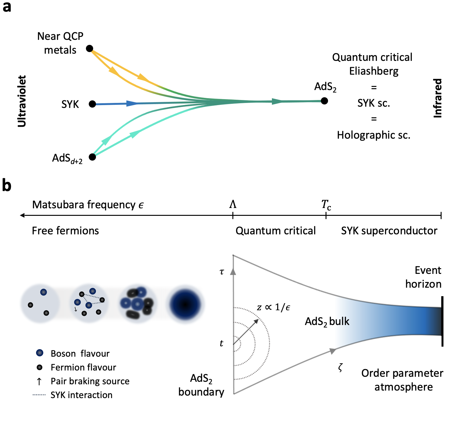
Figure 1: The emergence of the dual holographic theory from the SYK superconductor. Top a: The semi-universal low energy holographic action equal to quantum critical Eliashberg theory describing the IR of holographic superconductors (AdS_d+2), SYK superconductors, and metals near quantum critical points. Bottom b: Below the UV scale $\Lambda$, a strongly coupled quantum-critical fluid forms out of interacting fermions and bosons. Below this scale the fluctuating order parameter becomes a scalar field with emergent AdS₂ gravity and forms an atmosphere around a black hole event horizon. The frequency $\epsilon$ of the relative time $\tau_{1}-\tau_{2}$ and the absolute time $t=(\tau_{1}+\tau_{2})/2$ of SYK pairing fields $F\left(\tau_{1},\tau_{2}\right)=\frac{1}{N}\sum_{i=1}^{N}c_{i\uparrow}\left(\tau_{1}\right)c_{i\downarrow}\left(\tau_{2}\right)$ determine the set of geodesic half circles that span the anti-de Sitter space $(\tau,\zeta)$ on the gravity side.

A tremendous amount of new insight into quantum critical systems has been gained from a fundamentally different perspective given by the holographic dual formulation in terms of a higher-dimensional Anti-de Sitter (AdS) spaceZaanen2015 ; Ammon2015 ; Hartnoll2018 . This also extends to superconductivity. The holographic superconductor Hartnoll:2008vx ; Gubser:2008px can consistently describe order-parameter condensation in strongly coupled theories without quasiparticles and naturally encapsulates quantum critical points (QCPs) in addition to thermal transitions. Also here, these results are often pushed beyond the matrix large-$N$ theories for which holography is formally justified. Again, this should capture the most relevant dynamics, even though reliable quantitative information is in essence limited to systems where additional symmetries constrain the holographic model enough, e.g. the canonical example of $\mathcal{N}=4$ super Yang-Mills Maldacena:1997re , or, as of relevance here, the (0+1)-dimensional model of Sachdev-Ye-Kitaev (SYK) Sachdev1993 ; Sachdev2010 ; Kitaev2015 .

In this article we show how the mutually complementary regimes of quantum critical Eliashberg theory and holographic superconductivity actually overlap and are, in fact, different perspectives of the same identical physics. We derive holographic superconductivity in form of a gravity theory with emergent space-time from a quantum many-body Hamiltonian where the Eliashberg formalism is exact. To this end we focus on the quantum-critical transition to superconductivity in SYK-like models.

In the normal state, the SYK model is described by a low-energy effective action, the so-called Schwarzian theory, that can also be derived from two-dimensional gravity with a scalar field (the dilaton) Maldacena:2016hyu ; Maldacena:2016upp , where the same pattern of breaking of the conformal symmetry occurs. In fact, the structure of the Schwarzian action can be guessed with considerations of conformal symmetry alone. In stark contrast, our quantitative map between SYK-Eliashberg theory and holography clearly cannot and does not rely on conformal symmetry: the presence of an explicit scale, the critical temperature $T_{c}$, breaks scale-invariance, and the dynamical equation of order parameter formation is sensitive to certain details of the system. Instead, the SYK-Eliashberg dynamics and its exact holographic equivalent describe the semi-universal RG-flow; semi-universal in the sense that it is grounded in a universal quantum critical SYK superconducting transition in the infrared (IR), but may have different microscopic, ultraviolet (UV) origins. This is sketched in Fig. 1.

Using this exact map as an anchor, we exploit the power of holography to investigate the previously unknown dynamical pairing response of the SYK superconductor.

II From Eliashberg to holography

II.1 SYK-Eliashberg

The explicit example of Eliashberg theory for a tractable strongly coupled quantum critical point we shall focus on is the SYK superconductor constructed in ref.Esterlis2019 (see also Patel2018 ; Wang2019 ; Chowdhury2019 ; Hauck2020 ). This is a generalization of the complex SYK model with $N$ charge-$q$, spin-1/2 fermions $c_{i\sigma}$ and four-fermion interactions to a more generic Yukawa interaction with $M$ soft bosons $\phi_{k}$

$$H = -\mu\sum_{i=1,\sigma=\uparrow\downarrow}^{N}c_{i\sigma}^{\dagger}c_{i\sigma}+\frac{1}{2}\sum_{k=1}^{M}\left(\pi_{k}^{2}+\omega_{0}^{2}\phi_{k}^{2}\right)$$ (1)

$$+ \frac{1}{N}\sum_{ijk\sigma}^{M,N}\left(g_{ij,k}+g^{*}_{ji,k}\right)c_{i\sigma}^{\dagger}c_{j\sigma}\phi_{k}\,.$$

In essence it encodes fermions coupled to a large number of Einstein phonons at a common frequency $\omega_{0}$ in the strong coupling limit.

Disorder averaging over the interactions $g_{ij,k}$ around a zero mean can induce superconductivity in states without quasi-particles if $g_{ij,k}=(g_{k})_{ij}$ are sampled from the Gaussian Orthogonal Ensemble rather than the Gaussian Unitary Ensemble with variance $\bar{g}^{2}$. Interpolating between the two ensembles by introducing a pair-breaking parameter $0\leq\alpha\leq 1$ further allows to continuously vary the superconducting transition temperature $T_{\rm c}$ and tune it to vanish at a quantum critical pointHauck2020 .

These results follow after a rewriting of the path-integral in terms of bilocal propagator fields $G\left(\tau_{1},\tau_{2}\right)=\frac{1}{N}\sum_{i=1}^{N}c_{i\sigma}^{\dagger}\left(\tau_{1}\right)c_{i\sigma}\left(\tau_{2}\right)$ and $F\left(\tau_{1},\tau_{2}\right)=\frac{1}{N}\sum_{i=1}^{N}c_{i\uparrow}\left(\tau_{1}\right)c_{i\downarrow}\left(\tau_{2}\right)$ that correspond at the large-$N$ saddle point to the normal and anomalous Green’s function of the Nambu-Eliashberg formalism. Both have conjugate fields $\Sigma\left(\tau_{1},\tau_{2}\right)$ and $\Phi\left(\tau_{1},\tau_{2}\right)$ that play the role of self energies. The (Euclidean) action of the analysis is rather lengthy and can be found in the appendix. In the large $N,M$ limit with $M/N$ fixed, the equations of motion are recognized as strongly coupled Eliashberg equationsEsterlis2019 ; Patel2018 ; Wang2019 ; Chowdhury2019 ; Hauck2020 .

In the normal state $F(\tau_{1},\tau_{2})=\Phi(\tau_{1},\tau_{2})=0$, and the theory flows to a SYK critical state defined by the time-translation invariant scaling dynamics with fermion and boson propagators

$$G_{\rm n}(\tau_{1}-\tau_{2}) =b_{g}\frac{\tanh\left(\pi q{\cal E}\right)+\text{sign}(\tau_{1}-\tau_{2})}{|\tau_{1}-\tau_{2}|^{\frac{1+\gamma}{2}}},$$

$$D_{\rm n}(\tau_{1}-\tau_{2}) =b_{d}\frac{1}{|\tau_{1}-\tau_{2}|^{1-\gamma}}.$$ (2)

The exponent $0<\gamma<1$ can be tuned by varying the ratio $M/N$ and the charge density $n$ via Eq.(27) of the appendix. In the SYK literature one frequently uses $\Delta=(1+\gamma)/4$ instead of $\gamma$. The spectral asymmetry parameter ${\cal E}$ can be directly related to the particle density $n=\langle c_{i\sigma}^{\dagger}c_{i\sigma}\rangle$ via a generalized Luttinger theoremGeorges2001 ; Wang2020 , where ${\cal E}(n=1/2)=0$. It is also linked to the density dependence of the zero-point entropySachdev2015 $2\pi{\cal E}=\frac{\partial S_{0}}{\partial n}$. While the two coefficients $b_{g,d}$ depend on details of the UV behavior, the important combination $\mu_{\gamma}\equiv\bar{g}^{2}b_{d}b_{g}^{2}=\tfrac{\gamma}{4\pi}\cosh^{2}\left(\pi q{\cal E}\right)\tan\left(\pi\gamma/2\right)$ is dimensionless and universal. Thus, the normal state of the Hamiltonian (1) is a strongly coupled, quantum-critical fluid made of interacting fermions and bosons.

In the superconducting state in the vicinity of the phase transition $F$ and $\Phi$ remain small. We may then expand the action to second order and integrate out $\Phi$. This yields the leading contributions of superconducting fluctuations to the SYK action:

$$S^{\left({\rm sc}\right)}/N = \int_{\omega,\epsilon}\frac{F^{\dagger}\left(\omega,\epsilon\right)F\left(\omega,\epsilon\right)}{\Pi_{\rm n}\left(\omega,\epsilon\right)}$$

$$- \frac{\bar{g}^{2}\lambda_{p}}{2}\int_{\omega,\epsilon,\epsilon^{\prime}}F^{\dagger}\left(\omega,\epsilon\right)D_{\rm n}\left(\epsilon-\epsilon^{\prime}\right)F\left(\omega,\epsilon^{\prime}\right).$$

Here, we Fourier transformed $F\left(\tau_{1},\tau_{2}\right)$ with regards to the relative time $\tau_{1}-\tau_{2}$, with frequency $\epsilon$, and absolute time $t=\left(\tau_{1}+\tau_{2}\right)/2$, with frequency $\omega$, respectively. $\int_{\omega}\cdots=T\sum_{n}\cdots$ stands for the sum over Matsubara frequencies. $\lambda_{p}=\left(1-\alpha\right)M/N$ modifies the coupling constant in the pairing channel and depends on the pair breaking strength $\alpha$. The first term in Eq.(II.1) is determined by the particle-particle response function $\Pi_{\rm n}\left(\omega,\epsilon\right)=G_{\rm n}\left(\frac{\omega}{2}-\epsilon\right)G_{\rm n}\left(\epsilon+\frac{\omega}{2}\right)$ of the critical normal state. The second term contains the singular pairing interaction with boson propagator $D_{\rm n}\left(\epsilon\right)$.

Eq.(II.1) is then the IR effective action for the dynamic order parameter $F(\omega)_{\epsilon}=F(\omega,\epsilon)$ parametrized by a microscopic energy $\epsilon$. In the dynamics of BCS theory the $\epsilon$-dependence is neglected. The Eliashberg dynamics makes clear that $\epsilon$ is the relative energy of the fermions, and therefore representative of the characteristic energy at which the system is probed. One can indeed think of it as an RG scale, as our mapping to a holographic model will make clear.

II.2 Holographic map

Field-theory side	Gravity side
frequency $\epsilon$ of time lag $\tau_{1}-\tau_{2}$	holographic dimension $\zeta$
absolute time $(\tau_{1}+\tau_{2})/2$	time (Euclidean) $\tau$
anomalous propagator $F$	order parameter field $\psi$
fermion bubble $\Pi_{\rm n}(\omega,\epsilon)$	$\partial_{\tau}\psi$, mass contrib. $m_{(1)}^{2}>0$
pairing interaction $D_{\rm n}(\epsilon)$	$\partial_{\zeta}\psi$, mass contrib. $m_{(2)}^{2}<0$
Cooper pair charge $2q$	condensate charge $q_{\star}$
spectral asymmetry $\mathcal{E}$	$\text{AdS}_{2}$ electric field $E$

Table 1: Dictionary of the Eliashberg-gravity map. Summary of the correspondence between the degrees of freedom of the critical Eliashberg-SYK theory and those if (1+1)-dimensional holographic superconductor. Notice $\zeta$ and $\tau$ are related to $1/\epsilon$ and the abolute time by a Radon transformation.

Next we establish a holographic map based upon the effective action (II.1). We first consider the case $T=\mu=0$. It is convenient to only perform the Fourier transform $F\left(t,\epsilon\right)$ with respect to the relative time and keep the absolute time $t$. From the Pauli principle for singlet, even-frequency pairing follows that $F\left(t,\epsilon\right)$ does not depend on the sign of $\epsilon$. This allows us to introduce the scalar Bose field

$$\tilde{\psi}\left(t,z\right)=c_{0}z^{\frac{\gamma-1}{2}}F\left(t,c/z\right),$$ (4)

with $z=c\left|\epsilon\right|^{-1}$ and positive coefficients $c$ and $c_{0}$. Performing an inverse Radon transform $\tilde{\psi}\left(t,z\right)\rightarrow\psi\left(\tau,\zeta\right)$ – a necessity pointed out in Maldacena:2016hyu ; Das2018 – that maps pairs of points $(t,z)$ to a point $(\tau,\zeta)$ on an AdS₂ geodesic, at low energy it then follows that the SYK theory takes the form

$$S^{\left({\rm sc}\right)}/N=\int d\tau d\zeta\left(\frac{m^{2}}{\zeta^{2}}\left|\psi\right|^{2}+\left|\partial_{\tau}\psi\right|^{2}+\left|\partial_{\zeta}\psi\right|^{2}\right).$$ (5)

This is the the action of a holographic superconductor in AdS₂ with mass $m$ and with Euclidean signature:

$$ds^{2}=g_{ab}dx^{a}dx^{b}=\frac{1}{\zeta^{2}}\left(d\tau^{2}+d\zeta^{2}\right).$$ (6)

This derivation of a holographic map between SYK-Eliashberg and its AdS-dual, with the extra, radial direction $\zeta$ encoding the RG scale, is the central result of this paper. In the appendix we give further details on the derivation of Eq.(5), and give explicit expressions for the constants $c$ and $c_{0}$ as well as the mass $m$ in terms of the parameters of the Hamiltonian (1). The time derivative in Eq.(5) originates from the first term in Eq.(II.1) and is due to the $\omega$-dependence of the particle-particle bubble $\Pi_{\rm n}(\omega,\epsilon)$. The kinetic term in the radial direction of the holographic bulk is due to the singular pairing interaction $D_{\rm n}(\epsilon)$. Both terms contribute to the AdS₂ mass $m$. The anomalous power-law dependence $\Pi_{\rm n}(0,\epsilon)\sim|\epsilon|^{\gamma-1}$ yields a positive contribution $m_{\left(1\right)}^{2}\propto\lambda_{p}^{-1}$. Thus, particle-particle fluctuations act against superconductivity and reducing $\lambda_{p}$, further increases $m^{2}_{(1)}$. The finding $m^{2}_{(1)}>0$ reflects the absence of a naive Cooper instability in critical non-Fermi liquidsBalatsky1993 ; Sudbo1995 . However, the singular pairing interaction $D_{\rm n}(\epsilon)\sim|\epsilon|^{-\gamma}$ also leads to a negative contribution $m_{\left(2\right)}^{2}<-\tfrac{1}{4}$ that favors pairing. It is, by itself, always more negative than the AdS₂ Breitenlohner-Freedman (BF) bound $m_{{\rm BF}}^{2}=-\tfrac{1}{4}$ that signals the onset of an instability in AdS space Breitenlohner1982 . The zero-temperature phase transition takes place when $m^{2}=m_{\left(1\right)}^{2}+m_{\left(2\right)}^{2}$ equals $m_{{\rm BF}}^{2}$. This holographic condition is indeed identical to one obtained from an analysis of the Eliashberg equation in ref.Hauck2020 .

The holographic map was established at zero temperature. At finite temperature one must periodically identify time in the SYK action, or equivalently work with discrete Matsubara frequencies. Holography, on the other hand, prescribes that we must change the background space-time metric to that of an Euclidean AdS₂ black hole

$$ds^{2}=\frac{1}{\zeta^{2}}\left((1-\zeta^{2}/\zeta_{T}^{2})d\tau^{2}+\frac{1}{(1-\zeta^{2}/\zeta_{T}^{2})}d\zeta^{2}\right).$$ (7)

Here $\zeta_{T}^{-1}=2\pi T$ encodes the location of the black hole horizon. Because the normal state SYK physics in the IR is controlled by a conformal fixed point, the finite temperature theory at Euclidean time is mathematically directly related to the zero temperature oneKitaev2015 ; Sachdev2015 . The same is true in the AdS₂ theory: the black hole geometry is equivalent to the $T=0$ background after a coordinate transformationSachdev2019 . Tracing the transformation, the SYK model precisely translates to the finite $T$ version of the action (5) with metric Eq.(7), see appendix.

Finally we comment on the holographic map at finite chemical potential $\mu$. At low energies the normal state SYK model possesses an emergent U(1) symmetrySachdev2015 . It allows to relate the normal state fermion propagator at finite $\mu$ to the one for $\mu=0$. For $\Pi_{\rm n}(\omega,\epsilon)$ this amounts to the shift $\omega\to\omega-i4\pi q{\cal E}T$. On the other hand, the propagator of a charge $q^{*}$ scalar particle within AdS₂ that is exposed to a boundary electric field $E$, yields an analogous shift $\omega\rightarrow\omega-i2\pi q^{*}ET$.Faulkner:2009wj Hence, the holographic boundary electric field $E={\cal E}$ is given by the spectral asymmetry of the SYK model with effective charge $q^{*}=2q$ of the Cooper pair. Within the gauge $A_{\zeta}=0$ this yields the vector potential $A_{\tau}=\tfrac{{i}\cal E}{\zeta}\left(1-\zeta/\zeta_{T}\right)$.

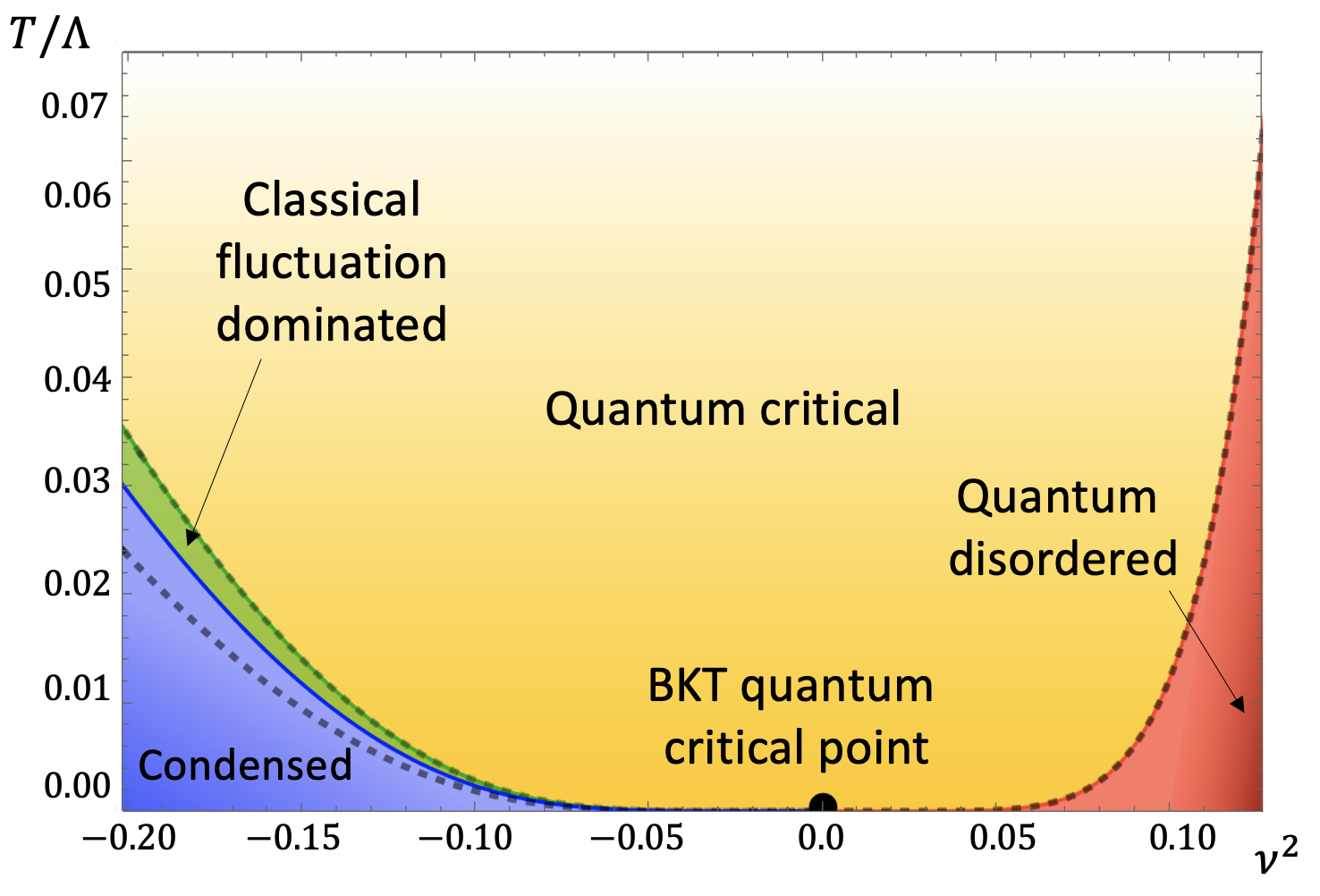
Figure 2: Phase diagram of the SYK model. Phase diagram as function of temperature $T$ and $\nu^{2}$ defined in Eq.(12) with $\gamma=0.9$. The susceptibility diverges at the transition temperature $T_{\rm c}$ (solid line) that vanishes in a BKT-like fashion at $\nu^{2}=0$. Below $T_{\rm c}$ we have superconducting order (blue). Between the dashed lines we find classical critical behavior with Curie-Weiss susceptibility and critical slowing down $\chi\sim t_{\rm dyn}\sim(T-T_{\rm c})^{-1}$ (we only calculated the upper dashed curve, the lower one is an educated guess). As the susceptibility is finite at the BKT quantum critical point, quantum criticality is identified by the regime where $\partial_{T}\chi(T)\sim 1/(T\log^{2}T)$ (yellow region). in the quantum disordered region (red) $\partial_{T}\chi(T)$ saturates as $T\rightarrow 0$. The quantum critical and quantum disordered regimes are separated by a crossover.

II.3 Pairing response

Though we have equated the actions, this only implies that the dynamical equations of motions match. For a true equivalent mapping the response to an external source field must also correspond. We can do so by checking an explicit observable, the order parameter susceptibility in the normal phase. We add an external pairing field $J_{0}(\tau)$ to the action:

$$S_{J}=-\int d\tau J_{0}\left(\tau\right)\sum_{i}c_{i\uparrow}\left(\tau\right)c_{i\downarrow}\left(\tau\right)+\text{h.c.}\,.$$ (8)

$J_{0}(\tau)$ is conjugate to the dynamic order parameter $\mathcal{O}(\tau)=\lim_{\tau^{\prime}\rightarrow\tau}\langle F(\tau,\tau^{\prime})\rangle$ and physically realizable via coupling through a Josephson junction. Using our holographic map this yields in the gravitational formulation $S_{J}=-\int d^{2}x\sqrt{g}\left(J(x)\psi^{*}(x)+h.c.\right)$ where at low frequencies $J\left(\tau,\zeta\right)=\frac{c}{c_{0}}\zeta^{\frac{1-\gamma}{2}}J_{0}\left(\tau\right)$. The corresponding Euler-Lagrange equation is

$$\partial_{\zeta}^{2}\psi+V\left(\omega,\zeta\right)\psi=\frac{J\left(\omega,\zeta\right)}{\zeta^{2}},$$ (9)

with potential $V\left(\omega,\zeta\right)=-\frac{m^{2}}{\zeta^{2}}+\left(i\omega{+}2q{\cal E}/\zeta\right)^{2}$. The $\zeta$-dependence on the r.h.s. of Eq.(9) ensures that the source term, formally present in the AdS-bulk, acts in essence only on the boundary, i.e. in the limit of small $\zeta$ dual to the UV, fully consistent with the holographic reasoning.

The Euler-Lagrange Eq.(9) should be identical to the stationary Eliashberg equation that follows from the original formulation of SYK model Eq.(II.1). Let us first consider a time independent source field $J_{0}$. Expressed in terms of the anomalous self energy $\Phi(\epsilon)=F\left(0,\epsilon\right)/\Pi_{\rm n}(0,\epsilon)$, the stationary equation for $F$ becomes

$$\Phi\left(\epsilon\right)=\lambda_{p}\bar{\mu}_{\gamma}\int_{\epsilon^{\prime}}\frac{\Phi\left(\epsilon^{\prime}\right)}{\left|\epsilon-\epsilon^{\prime}\right|^{\gamma}\left|\epsilon^{\prime}\right|^{1-\gamma}}+J_{0},$$ (10)

with $\bar{\mu}_{\gamma}$ given in the appendix. Interestingly, this equation is identical to the linearized gap equation of the Eliashberg theory of numerous quantum-critical metalsAbanov2001 ; Abanov2001b ; Chubukov2005 . Thus, our analysis goes beyond the specifics of the SYK model and is directly relevant to a much broader class of physical systems. The power-law behavior in Eq.(10) holds only within an upper (UV) and lower (IR) cut off $\Lambda$ and $T$, respectively. For $\left|\epsilon\right|\gg\Lambda$ the solution obviously becomes $\Phi\left(\epsilon\right)-J_{0}\propto\left|\epsilon\right|^{-\gamma}$, while at $\left|\epsilon\right|\ll T$ the anomalous self energy should approach a constant. This fixes the UV and IR boundary conditions $\left.\frac{d}{d\epsilon}\epsilon^{\gamma}\Phi\left(\epsilon\right)\right|_{\Lambda}=\gamma\Lambda^{\gamma-1}J_{0}$ and $\left.\frac{d}{d\epsilon}\Phi\left(\epsilon\right)\right|_{T}=0$. Hence, we do find that the source field acts through a UV boundary condition. As expected, the solution of the integral equation (10) and the much simpler Euler-Lagrange differential equation (9) at $\omega=0$ can be shown to be identical, provided we use the same boundary conditions. For small $\gamma$ it is in fact known that Eq.(10) can be formulated as a differential equationSon1999 ; Chubukov2005 ; Hauck2020 . Our conclusion is, however not limited to small $\gamma$.

The $\omega=0$ solution of Eq.(9) is

$$\psi\left(0,\zeta\right)=A\zeta^{\frac{1}{2}-\nu}+B\zeta^{\frac{1}{2}+\nu},$$ (11)

where $A$ and $B$ are determined by the boundary condition translated for $\psi(\omega,\zeta)$.

$$\nu^{2}=\frac{1}{4}+m^{2}-\left(2q{\cal E}\right)^{2}$$ (12)

is a convenient measure of the mass and charge that vanishes at the BF bound.

We can now easily determine the static susceptibility. Written with an eye on the holographic computations, it reads

$$\chi=\left.\frac{d{\cal O}}{dJ_{0}}\right|_{J_{0}=0}=\chi_{\mathrm{{c}}}\frac{b_{+}+b_{-}\mathcal{G}(T)\Lambda^{-2\nu}}{a_{+}+a_{-}\mathcal{G}(T)\Lambda^{-2\nu}},$$ (13)

where ${\cal G}\left(T\right)=c^{2\nu}\frac{B}{A}=\frac{2\nu-\gamma}{2\nu+\gamma}T^{2\nu}$ with $c$ from (4) contains the dependence on the IR behavior, while $a_{\pm}=b_{\pm}\left(1\pm 2\nu/\gamma\right)^{2}$ and $b_{\pm}=1\mp 2\nu/\gamma$ as well as $\chi_{\rm c}=2c_{g}^{2}\Lambda^{\gamma}/(\pi\gamma)$.

The static susceptibility determines the phase diagram of the model shown in Fig.2. The regime with superconducting order corresponds to $\nu$ being imaginary. In that case there are solutions for the order parameter obeying the source-less $J_{0}=0$ boundary conditions. This occurs whenever the denominator in Eq.(13) vanishes which determines the superconducting transition temperature:

$$T_{{\rm c}}\sim\Lambda e^{-\frac{\pi}{\sqrt{-\nu^{2}}}}.$$ (14)

In Fig.2 the ordered state is shown in blue. One recognizes a Berezinskii–Kosterlitz–Thouless (BKT) phase transitionKaplan2009 at a critical value of the pair-breaking parameter $\lambda_{p}$ that corresponds to $\nu=0$. Right above $T_{c}$ the susceptibility diverges according to the mean field Curie Weiss law $\chi(T)\sim(T-T_{\rm c})^{-1}$. This happens in the classical regime marked green in Fig.2. Note that at the BKT quantum criticial point the order parameter susceptibility is $\chi_{\rm c}$ and stays finite. This is in apparent contradiction with the behavior at quantum phase transitions, where commonly, the order parameter response to the external field is divergent. However, the milder BKT quantum criticality is signaled by a diverging slope of the susceptibility as it approaches this finite value $\partial_{T}\chi(\nu=0)\approx\tfrac{4\chi_{{\rm c}}}{\gamma T\log^{2}\left(\Lambda/T\right)}$ and $\partial_{\nu^{2}}\chi(T=0)\propto\chi_{\text{c}}/\nu$, fully consistent with results obtained from holography Iqbal:2011aj ; Jensen:2011af . The regime in the phase diagram where this is the behavior for $\partial_{T}\chi$ is indicated in yellow in Fig.2, while a saturation of the slope happens below the crossover to the quantum-disordered regime (marked red).

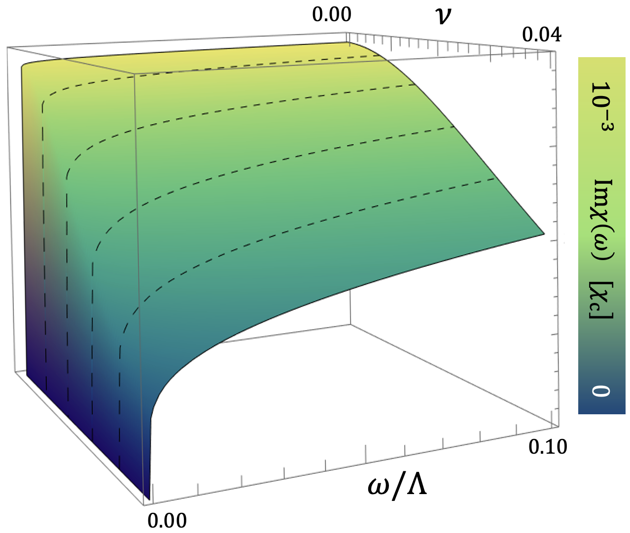
Figure 3: Dynamical susceptibility away from criticality. Imaginary part of the dynamic pairing susceptibility $\chi(\omega)$ for different values of the pair breaking, parametrized in terms of $\nu$ with $\gamma=0.01$ and $T/\Lambda=10^{-4}$. Notice the broad continuum right at the BKT quantum critical point that only decays like $1/\log^{2}\omega$ at lowest frequencies.

Eq.(13) is purposely written to be recognizable as identical to the susceptibility obtained from a holographic approach based on the crossover from a higher dimensional holographic theory AdS_d+2 at high energies to AdS${}_{2}\times\mathbb{R}^{d}$ at low energiesIqbal:2011aj ; Jensen:2011af . Below we discuss how the effect of the higher-dimensional space can be incorporated via appropriated double-trace deformations directly in the AdS₂ model Eq.(5) Zaanen2015 ; Witten2001 . This insight allows us to use the power of holography and determine the dynamic pairing susceptibility. Using the approach of refs. Iqbal:2011aj ; Jensen:2011af we obtain $\chi(\omega)$ immediately from the static susceptibility of Eq.(13) if we replace ${\cal G}\left(T\right)$ by

$${\cal G}\left(T,\omega\right)=\frac{2\nu-\gamma}{2\nu+\gamma}T^{2\nu}\frac{\Gamma\left(u-\nu\right)\Gamma\left(v+\nu\right)}{\Gamma\left(u+\nu\right)\Gamma\left(v-\nu\right)}$$ (15)

with $u=\tfrac{1}{2}+i2q{\cal E}$ and $v=\tfrac{1}{2}-i\tfrac{\omega-4\pi Tq{\cal E}}{2\pi T}$. Here we use retarded functions, i.e. in-falling boundary conditions at the black hole horizon Faulkner:2009wj . In Fig.3 we show the resulting frequency dependence of the imaginary part of the pairing susceptibility at low $T$ as function of $\omega$ for varying $\nu$. Most notable is the almost flat behavior right at the quantum critical point, where at lowest frequencies holds that ${\rm Im}\chi(\omega)\approx\tfrac{2\pi}{\gamma}\log^{-2}\left(\Lambda/\omega\right)$. This mirrors the temperature dependence discussed earlier. Near the classical transition at finite $T_{\rm c}$, we obtain critical slowing down behavior ${\rm Im}\chi(\omega)\sim\tfrac{\omega t_{\rm dyn}}{1+(\omega t_{\rm dyn})^{2}}$ with order-parameter relaxation time $t_{\rm dyn}\sim(T-T_{\rm c})^{-1}$. In Fig.4 we also show the impact of a deviation of the charge density from half filling, which induces a finite boundary electric field $\cal{E}$ and a spectral asymmetry of the two particle response.

Figure 4: Dynamical susceptibility away from charge neutrality. Real part of the dynamic pairing susceptibility $\chi(\omega)$ for different values of boundary electric fields ${\cal E}$ corresponding to different carrier density with $\gamma=0.01,\nu=10^{-3}$, and $T/\Lambda=10^{-2}$. Notice spectral asymmetry away from $n=1/2$.

Finally we establish a more direct connection between the susceptibility of the SYK model and holography in AdS₂ without having to resort to crossover argument from higher-dimensional gravitational spaces. To this end we need to posit the correct holographic boundary conditions for AdS₂. In holography, boundary conditions at $\zeta=0$ crucially encode the precise theory one describes beyond the physics of interest within that theory. For AdS₂ models this is a more detailed exercise, as the UV does not decouple as it does in higher dimensional theories Maldacena1999 , and further UV information is necessary to describe the theory. In brief: standard boundary conditions correspond to a theory where $A=\lim_{\zeta\rightarrow 0}\zeta^{\nu-\frac{1}{2}}\psi(\zeta)\equiv J_{0}$ with $J_{0}$ the external source conjugate to the operator of interest, and $B=\lim_{\zeta\rightarrow 0}\frac{\zeta^{1-2\nu}}{2\nu}\partial_{\zeta}\zeta^{\nu-\frac{1}{2}}\psi|_{\zeta=0}=\mathcal{O}$ as the response; alternative quantization boundary conditions correspond to $B=J_{0}$, $A=\mathcal{O}$; a dual theory with so-called double trace deformations corresponds to mixed boundary conditions of the type $B=fA+J_{0}$, $B=\mathcal{O}$, where $f$ is an arbitrary coupling constant, or in alternative quantizationZaanen2015 $A=fB+J_{0}$, $A=\mathcal{O}$. When the UV does not decouple, however, there is a new, fourth possibility, where one includes the contribution of the leading UV operator. This corresponds to mixed boundary conditions $B=fA+J_{0}$ and a mixed response $B=gA+\mathcal{O}$ with again $g$ an arbitrary constant. The susceptibility computed from AdS₂ isFaulkner:2009wj

$$\chi_{\text{AdS}_{2}}=\left.\frac{d{\cal O}}{dJ_{0}}\right|_{J_{0}=0}\simeq\frac{\mathcal{O}}{J_{0}}=\frac{B-gA}{B-fA}=\frac{1-g\mathcal{G}}{1-f\mathcal{G}}.$$ (16)

Up to normalization, this equals the holographic result obtained via dimensional crossoverFaulkner:2009wj and the SYK susceptibility Eq.(13).

III Summary

The low energy theory of the SYK Hamiltonian Eq.(1) can thus be formulated in terms of the action

$$S=S_{\rm gravity}+S_{\rm sc}+S_{J}.$$ (17)

$S_{\rm gravity}$ is the much discussed AdS gravity in $1+1$ dimensions which eventually gives rise to the Schwarzian theory, describing the SYK normal state Maldacena:2016hyu ; Maldacena:2016upp . It determines the metric of equations (6) and (7). Hence the non-Fermi liquid normal state provides the gravitational background. Superconducting degrees of freedom of the SYK model then behave like a charge $2q$ matter field on the AdS₂ background with:

$$S_{\rm sc}=N\int d^{2}x\sqrt{g}\left(D_{a}\psi^{*}D^{a}\psi+m^{2}\left|\psi\right|^{2}\right),$$ (18)

where $D_{a}=\partial_{a}{-}i2qA_{a}$. The finite temperature theory is equivalent to a change of coordinates that corresponds to a black hole with event horizon given by the Hawking temperature. Deviations of the density from half filling give rise to a boundary electric field ${\cal E}$. The competition between suppressed pairing due to the absence of quasi-particles and the enhanced, singular pairing interaction is merely a balance of two contributions to the mass $m$ and leads to a quantum critical point of the BKT variety. The Euler-Lagrange equation of the gravitational theory maps directly onto the Eliashberg equation intensely studied in the context of quantum critical metals. External fields that couple to Cooper pairs act on the AdS₂ boundary. We have therefore attained an explicit and complete AdS-field theory correspondence.

Our derivation of holographic superconductivity from a microscopic Hamiltonian allows for a deeper and more concrete understanding of the holographic principle. Our approach should be the natural starting point to study superconducting fluctuations beyond the Eliashberg limit and nonlinear effects, beyond the Gaussian level for systems as diverse as magnetic and nematic quantum critical points, or critical spin liquids. In the holographic language those effects correspond to quantum gravity corrections and gravitational back reactions, respectively. Moreover, as these systems are experimentally probedChowdhury2019 ; Chubukov2020 , it provides a direct avenue to test holography in the lab.

Appendix

A: SYK action of bilocal fields

In what follows we analyze the action of the SYK superconductor that follows from the Hamiltonian Eq.(1). As is common practice in the theory of SYK like models we use bilocal fields, i.e. collective field variables that depend on two time variables. The effective action of the superconducting Yukawa-SYK problem isEsterlis2019 ; Hauck2020 :

$$S = -N{\rm tr}\log\left(\hat{g}^{-1}-\hat{\Sigma}\right)+\frac{M}{2}{\rm tr}\log\left(d^{-1}-\Pi\right)$$ (19)

$$- N\left(G\otimes\Sigma+\widetilde{G}\otimes\widetilde{\Sigma}+F\otimes\Phi+F^{\dagger}\otimes\Phi^{\dagger}\right)+\frac{M}{2}D\otimes\Pi$$

$$- \frac{M}{2}\overline{g}^{2}\left((G\widetilde{G})\otimes D+\left(1-\alpha\right)\left(F^{\dagger}F\right)\otimes D\right),$$

with $M$ boson flavors and $N$ fermion flavors. We use the notation $A\otimes B=\int d\tau_{1}d\tau_{2}A\left(\tau_{1},\tau_{2}\right)B\left(\tau_{2},\tau_{1}\right)$ as well as $F^{\dagger}\left(\tau_{1},\tau_{2}\right)=F\left(\tau_{2},\tau_{1}\right)^{*}$ and $\widetilde{G}\left(\tau_{1},\tau_{2}\right)=-G\left(\tau_{2},\tau_{1}\right)$. The fermionic self energy and propagator are a matrices in Nambu space:

$$\hat{\Sigma}=\left(\begin{array}[]{cc}\Sigma&\Phi\\ \Phi^{\dagger}&\widetilde{\Sigma}\end{array}\right)\,\,\,{\rm and}\,\,\,\hat{G}=\left(\begin{array}[]{cc}G&F\\ F^{\dagger}&\widetilde{G}\end{array}\right).$$ (20)

The bare propagators are given as

$$\hat{g}^{-1}\left(\tau,\tau^{\prime}\right) = -\left(\partial_{\tau}\hat{\sigma}_{0}-\mu\hat{\sigma}_{z}\right)\delta\left(\tau-\tau^{\prime}\right),$$

$$d^{-1}\left(\tau,\tau^{\prime}\right) = -\left(\partial_{\tau}^{2}-\omega_{0}^{2}\right)\delta\left(\tau-\tau^{\prime}\right),$$ (21)

where the $\hat{\sigma}_{i}$ are $2\times 2$ Nambu-space matrices. For large $N$ and $M$, but fixed $N/M$ the exact solution of the single particle problem is given in terms of the stationary condition $\delta S=0$, which is given by the Eliashberg equations:

$$i\epsilon_{n}\left(1-Z\left(\epsilon_{n}\right)\right) = -\bar{g}^{2}\frac{M}{N}T\sum_{n^{\prime}}\frac{D\left(\epsilon_{n}-\epsilon_{n^{\prime}}\right)i\epsilon_{n^{\prime}}Z\left(\epsilon_{n^{\prime}}\right)}{\left(\epsilon_{n^{\prime}}Z\left(\epsilon_{n^{\prime}}\right)\right)^{2}+\Phi\left(\epsilon_{n^{\prime}}\right)^{2}},$$

$$\Phi\left(\epsilon_{n}\right) = \bar{g}^{2}\lambda_{p}T\sum_{n^{\prime}}\frac{D\left(\epsilon_{n}-\epsilon_{n^{\prime}}\right)\Phi\left(\epsilon_{n^{\prime}}\right)}{\left(\epsilon_{n^{\prime}}Z\left(\epsilon_{n^{\prime}}\right)\right)^{2}+\Phi\left(\epsilon_{n^{\prime}}\right)^{2}}.$$ (22)

Here, we considered $\mu=0$ and used $\hat{\Sigma}\left(\epsilon_{n}\right)=i\epsilon_{n}\left(1-Z\left(\epsilon_{n}\right)\right)\hat{\sigma}_{z}+\Phi\left(\epsilon_{n}\right)\hat{\sigma}_{x}$. This equation has to be supplemented by a corresponding expression for the boson self energyEsterlis2019 .

In the normal state the expectation values of $\Phi$ and $F$ vanish. Hence, near the superconducting transition we can expand for small $\Phi$ and $F$. This yields

$$S^{\left(sc\right)} = \Phi^{\dagger}\otimes G_{n}\otimes\Phi\otimes G_{n}-\frac{\bar{g}^{2}\lambda_{p}}{2}\left(F^{\dagger}F\right)\otimes D_{\rm n}$$ (23)

$$- F^{\dagger}\otimes\Phi-F\otimes\Phi^{\dagger}$$

where $G_{\rm n}$ and $D_{\rm n}$ are the finite temperature propagators of the normal state. If we now use that $G_{\rm n}$ and $D_{\rm n}$ only depend on the time difference, Fourier transform to frequency space, and integrate over the Gaussian fields $\Phi$ and $\Phi^{\dagger}$ we obtain Eq.(II.1) of the main text.

The particle number $n$ is related to the spectral asymmetry ${\cal E}$ though the generalized Luttinger theoremGeorges2001 ; Wang2020 :

$$n=\frac{1}{2}-\frac{\theta}{\pi}-\frac{1-\gamma}{4}\frac{\sin\left(2\theta\right)}{\cos\left(\pi\gamma/2\right)},$$ (24)

where $\tan\theta=\tan\left(\tfrac{\pi\left(1+\gamma\right)}{4}\right)\tanh\left(\pi q{\cal E}\right)$.

In the main text, we give in Eq.(II.1) the normal state propagators as function of time. Fourier transformation yields

$$G_{\rm n}\left(\epsilon\right) = c_{g}\left(\tan\theta+i{\rm sign}\left(\epsilon\right)\right)\left|\epsilon\right|^{-\frac{1-\gamma}{2}}$$

$$D_{\rm n}\left(\epsilon\right) = c_{d}\left|\epsilon\right|^{-\gamma}$$ (25)

where the coefficients are

$$c_{g} = 2b_{f}\Gamma\left(\tfrac{1-\gamma}{2}\right)\cos\left(\tfrac{\pi}{4}(1+\gamma)\right)$$

$$c_{d} = 2b_{b}\Gamma(\gamma)\cos(\pi\gamma/2),$$ (26)

and the exponent $\gamma$ is determined by

$$\frac{\left(1-\gamma\right)\tan\frac{\pi\left(1+\gamma\right)}{4}}{1+\tan^{2}\frac{\pi\left(1+\gamma\right)}{4}\tanh^{2}\left(\pi q{\cal E}\right)}=\frac{M}{N}\frac{\gamma\tan\frac{\pi\gamma}{2}}{1-\tanh^{2}\left(\pi q{\cal E}\right)}.$$ (27)

B: Derivation of the holographic map at $T=\mu=0$

First we summarize the derivation of Eqs.(4) and (5). The analysis is straightforward for the first term in Eq.(II.1). We expand the zero-temperature expression of $\Pi^{-1}\left(\omega,\epsilon\right)$ for small $\omega$ up to $\omega^{2}$:

$$\frac{1}{\Pi\left(\omega,\epsilon\right)} \approx \frac{1}{c_{g}^{2}}\left|\epsilon\right|^{1-\gamma}\left(1-\frac{1-\gamma}{8}\left(\frac{\omega}{\epsilon}\right)^{2}\right)$$ (28)

and Fourier transform from $\omega$ to Euclidean time $t$. One easily finds:

$$S^{\left({\rm sc},1\right)}/N = \int_{\omega,\epsilon}F^{\dagger}\left(\omega,\epsilon\right)\frac{1}{\Pi\left(\omega,\epsilon\right)}F\left(\omega,\epsilon\right)$$ (29)

$$= \int dzdt\left(\frac{m_{\left(1\right)}^{2}}{z^{2}}|\tilde{\psi}|^{2}-|\partial_{t}\tilde{\psi}|^{2}\right),$$

with $m_{\left(1\right)}^{2}=\frac{2\pi}{\lambda_{p}\bar{\mu}_{\gamma}b_{\gamma}}>0$. $b_{\gamma}$ will be defined below while

$$\bar{\mu}_{\gamma}=\mu_{\gamma}\Gamma\left(\gamma\right)\Gamma^{2}\left(\tfrac{1-\gamma}{2}\right)\left(2\cos\tfrac{\pi\gamma}{2}-\sin\left(\pi\gamma\right)\right).$$ (30)

$\mu_{\gamma}$ is given in the main text.

Next we analyze the second term

$$S_{{\rm SYK}}^{\left({\rm sc},2\right)}/N=-\frac{\bar{g}^{2}\lambda_{p}}{2}\int_{\omega,\epsilon,\epsilon^{\prime}}F^{\dagger}\left(\omega,\epsilon\right)D\left(\epsilon-\epsilon^{\prime}\right)F\left(\omega,\epsilon^{\prime}\right)$$ (31)

in Eq.(II.1). To proceed we perform a Mellin transform

$$F\left(\omega,\epsilon\right)=\int_{-\infty}^{\infty}\frac{dw}{\sqrt{2\pi}}f_{w}\left(\omega\right)\left|\epsilon\right|^{iw-1+\gamma/2}$$ (32)

and the second term in Eq.(II.1) becomes a set of uncoupled oscillators

$$S_{{\rm SYK}}^{\left({\rm sc},2\right)}/N=\bar{g}^{2}\lambda_{p}c_{d}\int_{\omega,w}r_{w}f_{w}^{*}\left(\omega\right)f_{w}\left(\omega\right),$$ (33)

where

$$r_{w} = \int_{-\infty}^{\infty}dx\frac{\left|x\right|^{iw}}{\left|1-x\right|^{\gamma}\left|x\right|^{1-\gamma/{2}}}$$

$$= \frac{\pi^{2}/2}{\Gamma\left(\gamma\right)\cos\left(\frac{\pi\gamma}{2}\right)\left|\sinh\left(\frac{\pi}{4}\left(2w-i\gamma\right)\right)\Gamma\left(1+iw-\frac{\gamma}{2}\right)\right|^{2}}.$$

Low energies corresponds to small $w$, where we can expand

$$r_{w}=a_{\gamma}-b_{\gamma}w^{2}$$ (35)

with positive coefficients

$$a_{\gamma} = \frac{\pi^{2}}{2\Gamma\left(\gamma\right)\cos\left(\frac{\pi\gamma}{2}\right)\left(\sin\left(\frac{\pi}{4}\gamma\right)\Gamma\left(1-\frac{\gamma}{2}\right)\right)^{2}},$$

$$b_{\gamma} = \frac{\pi^{2}\left(\pi^{2}-4\psi^{\left(1\right)}\left(1-\frac{\gamma}{2}\right)\sin^{2}\left(\frac{\pi\gamma}{4}\right)\right)}{8\Gamma\left(\gamma\right)\Gamma^{2}\left(1-\frac{\gamma}{2}\right)\sin^{4}\left(\frac{\pi\gamma}{4}\right)\cos\left(\frac{\pi\gamma}{2}\right)}.$$ (36)

Inverting the Mellin transform finally yields in terms of the scalar field of Eq.(4)

$$-\frac{\bar{g}^{2}\lambda_{p}}{2}\int_{\omega,\epsilon,\epsilon^{\prime}}F^{\dagger}DF=\int_{z,t}\left(\frac{m_{\left(2\right)}^{2}}{z^{2}}|\tilde{\psi}|^{2}+|\partial_{z}\tilde{\psi}|\right),$$ (37)

with $m_{\left(2\right)}^{2}=-\frac{1}{4}-a_{\gamma}/b_{\gamma}$. Finally, the two coefficients in Eq.(4) are

$$c_{0}^{2} = \frac{1-\gamma}{8\pi c_{g}^{2}}c^{-\gamma},$$

$$c^{2} = \frac{\pi}{4}\frac{1-\gamma}{b_{\gamma}\overline{\mu}_{\gamma}\lambda_{p}}.$$ (38)

This completes the derivation of the action in Lorentzian de Sitter space with mass $m^{2}=m^{2}_{(1)}+m^{2}_{(2)}$.

To transform the problem to AdS₂ we follow Ref.Das2018, and use the Radon transform which takes the explicit form

$$\tilde{\psi}\left(z,t\right) = \left({\cal R}\psi\right)(z,t)=2z\int_{t-z}^{t+z}d\tau\int_{0}^{\infty}\frac{d\zeta}{\zeta}\psi\left(\zeta,\tau\right)$$ (39)

$$\times \delta\left(z^{2}-\left(\tau-t\right)^{2}-\zeta^{2}\right).$$

If one now uses that one can relate the Laplacian before and after the Radon transformation $\Box_{{\rm dS}_{2}}{\cal R}\psi=-{\cal R}\left(\Box_{{\rm AdS}_{2}}\psi\right)$ it follows that the Radon transform $\tilde{\eta}_{\lambda}={\cal R}\eta_{\lambda}$ of an eigenfunction $\eta_{\lambda}$ of the Laplacian in AdS₂ is also an eigenfunction of $\Box_{{\rm dS}_{2}}$. It is however not normalized. Addressing this issue through so-called leg factorsDas2018 one obtains at low energy the action (5) in AdS₂ with modified mass

$$\bar{m}{}^{2}=m_{{\rm BF}}^{2}+\frac{m^{2}-m_{{\rm BF}}^{2}}{\left[1-4G\left(m^{2}-m_{{\rm BF}}^{2}\right)\right]}.$$ (40)

$G=\sum_{n=0}^{\infty}\frac{\left(-1\right)^{n}}{\left(2n+1\right)^{2}}\approx 0.915966$ is Catalan’s constant. Near the Breitenlohner-Freedman bound $m^{2}_{\rm BF}=\tfrac{1}{4}$ both masses are the same, which is the reason why we did not distinguish between $m$ and $\bar{m}$ in the main text. This completes the holographic map.

If we specify the density $n$, the ratio of boson and fermion flavors $M/N$, and the pair-breaking strength $\alpha$ the three crucial quantities ${\cal E}$, $\gamma$ and $\lambda_{p}$ are fixed and the gravitational theory is well defined. Only one number - in our case $b_{g}$ - has to be fixed from a numerical solution of the SYK model. However it only determines the global factor $c_{0}$ of the holographic action.

C: Holographic map at finite temperatures

In the analysis at finite temperatures we start from the action for the SYK-superconductor Eq.(23) without integrating out the conjugate field $\Phi\left(\tau_{1},\tau_{2}\right)$. We have to keep in mind that the time integrations go from $-\beta/2$ to $\beta/2$ where $\beta=1/T$. Similarly, $G_{{\rm n}}$ and $D_{{\rm n}}$ are the finite temperature propagators of the normal state. Using the invariance of the low-energy saddle point equations under re-parametrization $\tau\rightarrow\bar{\tau}=f\left(\tau\right)$, both functions can be obtained from the $T=0$ solutions $G_{{\rm n},0}\left(\tau\right)$ and $D_{{\rm n},0}\left(\tau\right)$ via

$$G_{\rm n}\left(\tau,\tau^{\prime}\right) = f^{\prime}\left(\tau\right)^{\frac{1+\gamma}{4}}G_{{\rm n},0}\left(f\left(\tau\right)-f\left(\tau^{\prime}\right)\right)f^{\prime}\left(\tau^{\prime}\right)^{\frac{1+\gamma}{4}},$$

$$D_{\rm n}\left(\tau,\tau^{\prime}\right) = f^{\prime}\left(\tau\right)^{\frac{1-\gamma}{2}}D_{{\rm n},0}\left(f\left(\tau\right)-f\left(\tau^{\prime}\right)\right)f^{\prime}\left(\tau^{\prime}\right)^{\frac{1-\gamma}{2}},$$

with $f\left(\tau\right)=\frac{\beta}{\pi}\tan\left(\frac{\pi\tau}{\beta}\right)$. Hence, the finite temperature problem leads to an effective action, identical to the one we analyzed at $T=0$, yet in terms of the field

$$\bar{F}\left(\bar{\tau}_{1},\bar{\tau}_{2}\right) = \left(1+\left(\pi T\right)^{2}\bar{\tau}_{1}^{2}\right)^{-\frac{1+\gamma}{4}}\left(1+\left(\pi T\right)^{2}\bar{\tau}_{2}^{2}\right)^{-\frac{1+\gamma}{4}}$$ (41)

$$\times F\left(f^{-1}\left(\bar{\tau}_{1}\right),f^{-1}\left(\bar{\tau}_{2}\right)\right)$$

Hence, we can immediately make the identification that is analogous to Eq.(4) only in terms of the new function $\bar{F}$ instead of $F$ and with transformed variable $\bar{\tau}_{1,2}$ instead of $\tau_{1,2}$. The scalar field, expressed in terms of the anomalous propagator field, that replaces (4) at finite temperatures is then:

$$\tilde{\psi}(\bar{t},\bar{z}) = c_{0}|\bar{\zeta}|^{\frac{1-\gamma}{2}}\int_{-\infty}^{\infty}ds\bar{F}\left(t_{+},t_{-}\right)e^{ics/\bar{x}},$$ (42)

where $t_{\pm}=\bar{t}\pm\frac{s}{2}$. After performing an inverse Radon transformation from $\tilde{\psi}(\bar{t},\bar{z})$ to $\psi(\bar{\tau},\bar{\zeta})$, the holographic action can now be transformed from coordinates $(\bar{\tau},\bar{\zeta})$ to $\left(\tau,\zeta\right)$, where $0<\tau<1/T$, which agrees at the boundary with the original imaginary variables of the SYK modelSachdev2019

$$\bar{\tau} = 2\zeta_{T}\frac{\left(1-\zeta^{2}/\zeta_{T}^{2}\right)^{1/2}\sin\left(\tau/\zeta_{T}\right)}{1+\left(1-\zeta^{2}/\zeta_{T}^{2}\right)^{1/2}\cos\left(\tau/\zeta_{T}\right)},$$

$$\bar{\zeta} = \frac{2\zeta}{1+\left(1-\zeta^{2}/\zeta_{T}^{2}\right)^{1/2}\cos\left(\tau/\zeta_{T}\right)}.$$ (43)

where $\zeta_{T}=\tfrac{1}{2\pi T}$. In these coordinates the finite-$T$ action of the SYK superconductor becomes

$$S^{\left({\rm sc}\right)}/N = \int_{0}^{\zeta_{0}}d\zeta\int_{-\beta/2}^{\beta/2}d\tau\left(\frac{m^{2}}{\zeta^{2}}\psi^{*}\psi+\frac{\partial_{\tau}\psi^{*}\partial_{\tau}\psi}{1-\zeta^{2}/\zeta_{T}^{2}}\right.$$ (44)

$$+ \left.\left(1-\zeta^{2}/\zeta_{T}^{2}\right)\partial_{\zeta}\psi^{*}\partial_{\zeta}\psi\right),$$

which is the correct finite-$T$ version of a holographic superconductor in AdS₂ with black hole horizon $\zeta_{T}$ and metric Eq.(7).

References

- (1) Eliashberg, G. M. Interactions between electrons and lattice vibrations in a superconductor. Sov. Phys. JETP 11, 696 (1960).
- (2) Eliashberg, G. M. Temperature Green’s functions for electrons in a superconductor. Sov. Phys. JETP 12, 1000 (1961).
- (3) Mathur, N. D. et al. Magnetically mediated superconductivity in heavy fermion compounds. Nature 394, 39 (1998).
- (4) Kasahara, S. et al. Evolution from non-Fermi-to Fermi-liquid transport via isovalent doping in BaFe2(As1-xPx)2 superconductors. Phys. Rev. B 81, 184519 (2010).
- (5) Sachdev, S. & Keimer B. Quantum Criticality. Physics Today 64N2, 29 (2011).
- (6) Balatsky, A. V. Superconducting instability in a non-Fermi liquid scaling approach. Philos. Mag. Lett. 68, 251 (1993).
- (7) Sudbø, A. Pair Susceptibilities and Gap Equations in Non-Fermi Liquids. Phys. Rev. B 74, 2575 (1995).
- (8) Abanov, Ar., Chubukov, A. & Finkel’stein, A. Coherent vs. incoherent pairing in 2D systems near magnetic instability. Europhys. Lett. 54, 488 (2001).
- (9) Abanov, Ar. , Chubukov, A. V. & Schmalian J. Quantum-critical superconductivity in underdoped cuprates. Europhys. Lett. 55, 369 (2001).
- (10) Chubukov, A. V. & Schmalian J. Superconductivity due to massless boson exchange in the strong-coupling limit Phys. Rev. B 72, 174520 (2005).
- (11) She, J.-H. & Zaanen, J. BCS superconductivity in quantum critical metals. Phys. Rev. B 80, 184518 (2009).
- (12) She, J.-H. et al. Observing the origin of superconductivity in quantum critical metals. Phys. Rev. B 84, 144527 (2011).
- (13) Abanov, A. & Chubukov, A. V. Interplay between superconductivity and non-Fermi liquid at a quantum critical point in a metal. I. The -model and its phase diagram at : The case . Phys. Rev. B 102, 024524 (2020).
- (14) Wu, Y.-M., Abanov, A. & Chubukov, A. V. Interplay between superconductivity and non-Fermi liquid at a quantum critical point in a metal. II. The -model at finite for . Phys. Rev. B 102, 024525 (2020).
- (15) Bonesteel, N. E., McDonald, I. A. & Nayak, C. Gauge Fields and Pairing in Double-Layer Composite Fermion Metals. Phys. Rev. Lett. 77, 3009 (1996).
- (16) Metlitski, M. A., Mross, D. F., Sachdev, S. & Senthil,T. Cooper pairing in non-Fermi liquids. Phys. Rev. B 91, 115111 (2015).
- (17) Son, D. T. Superconductivity by long-range color magnetic interaction in high-density quark matter. Phys. Rev.D 59, 094019 (1999).
- (18) Roussev, R. & Millis, A. J. Quantum critical effects on transition temperature of magnetically mediated p-wave superconductivity. Phys. Rev. B 63, 140504R (2001).
- (19) Raghu, S., Torroba, G. & Wang, H. Metallic quantum critical points with finite BCS couplings. Phys. Rev. B 92, 205104 (2015).
- (20) Chowdhury, D & Berg, E. The unreasonable effectiveness of Eliashberg theory for pairing of non-Fermi liquids, Annals of Physics 417, 168125 (2020).
- (21) Chubukov, A. V. , Abanov, A., Esterlis, I. & Kivelson, S. A. Eliashberg theory of phonon-mediated superconductivity — when it is valid and how it breaks down. Ann. Physics 417, 168190 (2020).
- (22) Zaanen, J. ,Liu, Y. , Sun, Y.-W. & Schalm, K. Holographic Duality in Condensed Matter Physics (Cambdrige Univ. Press, Cambridge, UK, 2015).
- (23) Ammon, M. & Erdmenger, J. Gauge/Gravity Duality: Foundations and Applications (Cambridge University Press, Cambridge, UK, 2015).
- (24) Hartnoll, S. A. , Lucas, A. & Sachdev S. Holographic Quantum Matter ( The MIT Press, Cambridge, Massachusetts and London, England, 2018).
- (25) Gubser, S. S. Breaking an Abelian gauge symmetry near a black hole horizon. Phys. Rev. D 78, 065034 (2008).
- (26) Hartnoll, S. A., Herzog, C. P. & Horowitz, G. T. Building a Holographic Superconductor. Phys. Rev. Lett. 101, 031601 (2008).
- (27) Maldacena, J. The Large N limit of superconformal field theories and supergravity. Adv. Theor. Math. Phys. 2 231 (1998).
- (28) Sachdev, S. & Ye, J. Gapless spin liquid ground state in a random, quantum Heisenberg magnet. Phys. Rev. Lett. 70, 3339, (1993).
- (29) Sachdev, S. Holographic Metals and the Fractionalized Fermi Liquid. Phys. Rev. Lett. 105, 151602 (2010).
- (30) Kitaev, A. A simple model of quantum holography. Talk at http://online.kitp.ucsb.edu/online/entangled15/kitaev/ and http://online.kitp.ucsb.edu/online/entangled15/kitaev2/ (2015).
- (31) Maldacena, J. & Stanford, D. Remarks on the Sachdev-Ye-Kitaev model. Phys. Rev. D 94, no.10, 106002 (2016).
- (32) Maldacena, J., Stanford, D., & Yang, Z. Conformal symmetry and its breaking in two dimensional Nearly Anti-de-Sitter space. PTEP 2016, no.12, 12C104 (2016).
- (33) Myers, R. C., Sierens. T. & Witczak-Krempa, W. A Holographic Model for Quantum Critical Responses. JHEP 05, 073 (2016).
- (34) Esterlis, I. & Schmalian, J. Cooper pairing of incoherent electrons: An electron-phonon version of the Sachdev-Ye-Kitaev model. Phys. Rev. B 100, 115132 (2019).
- (35) Patel, A. A., Lawler, M. J. & Kim, E.-A. Coherent Superconductivity with a Large Gap Ratio from Incoherent Metals. Phys. Rev. Lett. 121, 187001 (2018).
- (36) Wang, Y. Solvable Strong-coupling Quantum Dot Model with a Non-Fermi-liquid Pairing Transition. Phys. Rev. Lett. 124, 017002 (2020).
- (37) Chowdhury, D. & Berg, E. Intrinsic superconducting instabilities of a solvable model for an incoherent metal. Phys. Rev. Res. 2, 013301 (2020)
- (38) Hauck, D., Klug, M. J., Esterlis, I. & Schmalian, J. Eliashberg equations for an electron–phonon version of the Sachdev–Ye–Kitaev model: Pair breaking in non-Fermi liquid superconductors. Ann. Physics 417, 168120 (2020).
- (39) Georges, A., Parcollet, O. & Sachdev, S. Quantum fluctuations of a nearly critical Heisenberg spin glass. Phys. Rev. B 63 134406 (2001).
- (40) Wang, Y. & Chubukov, A. V. Quantum phase transition in the Yukawa-SYK model. Phys. Rev. Res. 2, 033084 (2020).
- (41) Sachdev, S. Bekenstein-Hawking Entropy and Strange Metals. Phys. Rev. X 5, 041025 (2015).
- (42) Das, R., Ghosh, A., Jevicki, A., & Suzuki, K. Space-time in the SYK model. JHEP 07, 184 (2018).
- (43) Breitenlohner, P. & Freedman, D. Z. Stability in gauged extended supergravity. Ann. Phys 144, 249 (1982).
- (44) Sachdev, S. Universal low temperature theory of charged black holes with AdS2 horizons. J. Math. Phys. 60, 052303 (2019).
- (45) Faulkner, T., Liu, H., McGreevy, J., Vegh, D. Emergent quantum criticality, Fermi surfaces, and AdS2. Phys. Rev. D 83, 125002 (2011).
- (46) Kaplan, D. B., Lee, J.-W., Son, D. T. & Stephanov, M. A. Conformality lost. Phys. Rev. D 80, 125005 (2009).
- (47) Iqbal, N., Liu, H. & Mezei, M. Quantum phase transitions in semilocal quantum liquids. Phys. Rev. D 91, no.2, 025024 (2015).
- (48) Jensen, K. Semi-Holographic Quantum Criticality. Phys. Rev. Lett. 107, 231601 (2011).
- (49) Witten, E. Multi-Trace Operators, Boundary Conditions, And AdS/CFT Correspondence. Preprint at https://arxiv.org/abs/hep-th/0112258 (2014).
- (50) Maldacena, J., Michelson, J. & Strominger, A. Anti-de Sitter Fragmentation. JHEP 9902,011(1999).