New bounds on adaptive quantum metrology under Markovian noise

Abstract

We analyse the problem of estimating a scalar parameter $g$ that controls the Hamiltonian of a quantum system subject to Markovian noise. Specifically, we place bounds on the growth rate of the quantum Fisher information with respect to $g$, in terms of the Lindblad operators and the $g$-derivative of the Hamiltonian $H$. Our new bounds are not only more generally applicable than those in the literature—for example, they apply to systems with time-dependent Hamiltonians and/or Lindblad operators, and to infinite-dimensional systems such as oscillators—but are also tighter in the settings where previous bounds do apply. We derive our bounds directly from the master equation describing the system, without needing to discretise its time evolution. We also use our results to investigate how sensitive a single detection system can be to signals with different time dependences. We demonstrate that the sensitivity bandwidth is related to the quantum fluctuations of $\partial H/\partial g$, illustrating how ‘non-classical’ states can enhance the range of signals that a system is sensitive to, even when they cannot increase its peak sensitivity.

I Introduction

Many metrological problems take the form of detecting a small, effectively classical influence acting on a system. Examples include standard tasks such as radio wave detection, magnetometry, and accelerometry, as well as problems in fundamental physics such as gravitational wave detection and searches for new forces.

For real-world apparatuses, the sensitivity to small signals is often constrained by practical noise sources such as vibrations, or by sources of uncertainties such as fabrication errors. However, in some cases, it is possible to suppress these issues to the point where the fundamental limits imposed by quantum mechanics become important. For example, at high enough frequencies, the dominant noise source in the LIGO gravitational wave detectors is quantum shot noise Saulson (1994). In order to determine how best to conduct measurements, it is therefore important to understand the quantum mechanical limits on signal detection.

If our detector system is under perfect control, then there is a simple answer to this question. We will model a ‘classical’ influence acting on a quantum system as a c-number parameter that affects the system’s Hamiltonian $H$. For a single real parameter $g$, the distinguishability of different values is set by the ‘quantum Cramér-Rao bound’ (also referred to as the ‘fundamental quantum limit’, or FQL) Giovannetti et al. (2011), in terms of the quantum fluctuations of $H^{\prime}\equiv\partial H/\partial g$. The FQL has been used to analyse systems including gravitational wave detection experiments Miao et al. (2017); Pang and Chen (2019) and axion dark matter detection experiments Lasenby (2021), providing insights into their sensitivity limits.

However, in many cases, a detector system is coupled to a complicated environment, which can prevent us from reaching the FQL sensitivity. A range of papers in the quantum metrology literature have investigated sensitivity limits under various different assumptions about the environment and its coupling to the detector system.

A common and useful approximation takes the environment to be a Markovian bath, in which case the evolution of the detector system is governed by a Lindblad master equation Wiseman and Milburn (2009). This was examined in a number of recent papers Sekatski et al. (2017); Demkowicz-Dobrzański et al. (2017); Zhou et al. (2018); Zhou and Jiang (2020), which considered parameter estimation for a time-independent $H^{\prime}$ acting on a finite-dimensional detector system. They found that if $H^{\prime}$ can be written as a suitable combination of the Lindblad operators associated with the coupling to the environment, then the sensitivity to $g$—quantified by the quantum Fisher information (QFI)—scales at best linearly over large times. Conversely, if this condition is not satisfied, the QFI can grow as $\sim\!t^{2}$.

In this paper, we analyse Hamiltonian parameter estimation for a system evolving according to a Markovian master equation, without assuming time-independence or finite dimensionality. We derive bounds on the growth rate of the QFI; in the case of finite-dimensional systems with time-independent $H^{\prime}$ and Lindblad operators, these sharpen the previously derived limits. Our new bounds also apply more broadly, including to infinite-dimensional systems such as oscillators, and to time-dependent $H^{\prime}$ and Lindblad terms. Similarly to Sekatski et al. (2017); Demkowicz-Dobrzański et al. (2017); Zhou et al. (2018); Zhou and Jiang (2020), they encompass detection schemes involving general adaptive strategies.

We arrive at our bounds using different methods from those in prior work. Unlike previous analyses, our derivation does not rely on discretising the time evolution of the system. Instead, we use symmetric logarithmic derivatives to directly bound the time derivative of the QFI starting from the master equation, enabling a fully time-dependent treatment. We compare our results in detail to existing bounds, showing that ours are tighter even in the restricted settings where the latter apply.

Being able to analyse time-dependent signals allows us to address additional metrological questions. The QFI assumes a signal that depends on a single real parameter $g$; in particular, the time dependence of the signal (for given $g$) is assumed to be known. However, in many situations, we are interested in a whole range of possible signals, with different time dependences. Examples include signals with a priori unknown frequency, such as axion dark matter with an unknown mass Graham et al. (2015), or gravitational waves from a pulsar of unknown spin rate Lasky (2015).

In such cases, we are interested in both the peak sensitivity at the optimal frequency, and the bandwidth over which we can (approximately) attain this sensitivity. We demonstrate that, in a range of different situations, the sensitivity bandwidth can be related to the short-time growth rate of the QFI, which itself is related to the quantum fluctuations of $H^{\prime}$. Consequently, using states with enhanced fluctuations can increase the sensitivity bandwidth, even when the noise terms prevent this from increasing the peak sensitivity.

For example, if we consider the problem of near-resonant force detection—detecting a small classical forcing acting on a damped harmonic oscillator—then there is a state-independent bound on the sensitivity. This can be attained, for an on-resonance forcing, by a critically-coupled oscillator in its ground state. Using ‘non-classical’ states, such as squeezed states or Fock states, cannot improve this peak sensitivity (assuming Markovian damping). However, such states can have larger $H^{\prime}$ fluctuations, and correspondingly, can enhance the bandwidth over which near-peak sensitivities can be achieved. This behaviour has been noted for schemes using squeezed coherent states Malnou et al. (2019)—we show that it applies more generally.

II Hamiltonian parameter estimation

We will suppose that we have some quantum system that can be described by a master equation in Lindblad form Nielsen and Chuang (2011); Wiseman and Milburn (2009),

$$\dot{\rho}=-i[H,\rho]+\sum_{j}\Big{(}L_{j}\rho L_{j}^{\dagger}-\frac{1}{2}\left\{L_{j}^{\dagger}L_{j},\rho\right\}\Big{)},$$ (1)

where $\rho$ is the system’s density operator, $H$ is its Hamiltonian, the $L_{j}$ are Lindblad operators describing its interaction with a Markovian environment, and $\dot{\rho}\equiv\partial\rho/\partial t$ is the time derivative of $\rho$. We assume that $H$ depends on some c-number parameter $g\in\mathbb{R}$ that we are trying to determine. For instance, $g$ might correspond to the strength of the signal. A simple but illustrative setup of this kind is a two-level system with a $g$-dependent energy splitting, $H=g\epsilon\sigma_{z}$, subject to dephasing noise, which is described by a single Lindblad operator $L_{1}=\sqrt{\gamma}\sigma_{z}$:

$$\dot{\rho}=-ig\epsilon[\sigma_{z},\rho]+\gamma(\sigma_{z}\rho\sigma_{z}-\rho).$$ (2)

Henceforth, all operators are functions of $t$ and $g$ in general, except for the Lindblad operators, which depend only on $t$. We suppress the $t$- and $g$- dependence of operators as well as scalar quantities in many equations; unless noted otherwise, these equations hold for all values of $t$ and $g$. Throughout, we use over-dots to denote differentiation with respect to $t$, and primes to denote differentiation with respect to $g$.

Given $\rho(t_{0},g)$ as a function of $g$ for a fixed time $t_{0}$, the master equation (Eq. (1)) tells us the state $\rho(t,g)$ at later times $t$. The distinguishability of different $g$ values can be quantified via the quantum Fisher information (QFI), which is the maximum, over different measurements, of the classical Fisher information (with respect to $g$) of the measurement outcome Braunstein and Caves (1994). The quantum Cramér-Rao bound (QCRB) states that the uncertainty $\delta g$ in measuring $g$ is bounded as $\delta g\geq 1/\sqrt{n\mathcal{F}}$, where $\mathcal{F}$ is the QFI and $n$ is the number of repetitions of the experiment (specifically, the QCRB lower-bounds the variance of any unbiased estimator of $g$; this bound can always be attained in the large-$n$ limit) Braunstein and Caves (1994).

II.1 General QFI bounds

For given $\rho=\rho(t,g)$, a useful quantity to define is the ‘symmetric logarithmic derivative’ (SLD) $\mathcal{L}=\mathcal{L}(t,g)$, which is a Hermitian operator with the property that

$$\rho^{\prime}=\frac{1}{2}\left(\rho\mathcal{L}+\mathcal{L}\rho\right).$$ (3)

(As we show in Appendix A, if it is possible to find $\mathcal{L}(t_{0},g)$ at some time $t_{0}$, then it is always possible to find $\mathcal{L}(t,g)$ at later times.) The QFI is then given by Braunstein and Caves (1994)

$$\mathcal{F}=\operatorname{tr}\left(\rho\mathcal{L}^{2}\right).$$ (4)

Under the assumption that $\rho,\rho^{\prime}$ and $\mathcal{L}$, are differentiable with respect to time,

$$\dot{\mathcal{F}}=\operatorname{tr}\left(\dot{\rho}\mathcal{L}^{2}+\rho\dot{\mathcal{L}}\mathcal{L}+\rho\mathcal{L}\dot{\mathcal{L}}\right),$$ (5)

which can be written using Eq. (3) as Lu et al. (2010)

$$\dot{\mathcal{F}}=2\operatorname{tr}\left(\dot{\rho}^{\prime}\mathcal{L}\right)-\operatorname{tr}\left(\dot{\rho}\mathcal{L}^{2}\right).$$ (6)

This form allows us to use the master equation expression for $\dot{\rho}$ (Eq. (1)); after some algebra, we obtain

$$\dot{\mathcal{F}}=2i\operatorname{tr}\left(\rho[H^{\prime},\mathcal{L}]\right)-\sum_{j}\operatorname{tr}\left(\rho[L_{j},\mathcal{L}]^{\dagger}[L_{j},\mathcal{L}]\right).$$ (7)

Note that this expression depends only on $H^{\prime}$, and not on $H$. This is to be expected, since $g$-independent evolution cannot contribute to distinguishing between different values of $g$.

Next, to bound $\dot{\mathcal{F}}$, it is helpful to subtract combinations of the Lindblad operators $L_{j}$ from $H^{\prime}$. Specifically, for any scalar coefficients $\alpha\in\mathbb{R}$ and $\beta_{j},\gamma_{jk}\in\mathbb{C}$ with $\gamma_{jk}=\gamma_{kj}^{*}$ (where the indices $j,k$ run over the same range as for the Lindblad operators), we can write

$$H^{\prime}=G+\alpha I+\sum_{j}(\beta_{j}^{*}L_{j}+\beta_{j}L_{j}^{\dagger})+\sum_{j,k}\gamma_{jk}L_{j}^{\dagger}L_{k}$$ (8)

for some Hermitian operator $G$. (Recall that the $t$- and $g$-dependence of operators is implicit; similarly, the coefficients $\alpha,\beta_{j},\gamma_{jk}$ are allowed to vary with $t$ and $g$.) Then,

$$i[H^{\prime},\mathcal{L}] =i[G,\mathcal{L}]+\sum_{j}\left[i\Big{(}\beta^{*}_{j}+\sum_{k}\gamma_{kj}L_{k}^{\dagger}\Big{)}[L_{j},\mathcal{L}]+{\rm h.c.}\right]$$

$$=i[G,\mathcal{L}]+\sum_{j}\left(A_{j}^{\dagger}[L_{j},\mathcal{L}]+{\rm h.c.}\right)$$ (9)

where we define

$$A_{j}\coloneqq i\left(\beta_{j}I+\sum_{k}\gamma_{jk}L_{k}\right).$$ (10)

Substituting Eq. (9) into Eq. (7), we have

$$\dot{\mathcal{F}} =2i\operatorname{tr}(\rho[G,\mathcal{L}])+4\sum_{j}\mathrm{Re}\left[\operatorname{tr}(\rho A_{j}^{\dagger}[L_{j},\mathcal{L}])\right]$$

$$\quad-\sum_{j}\operatorname{tr}\left(\rho[L_{j},\mathcal{L}]^{\dagger}[L_{j},\mathcal{L}]\right)$$ (11)

$$\leq 2i\operatorname{tr}\left(\rho[G,\mathcal{L}]\right)$$

$$\quad+4\sum_{j}\left\{\sqrt{\operatorname{tr}(\rho A_{j}^{\dagger}A_{j})}\sqrt{\operatorname{tr}\left(\rho[L_{j},\mathcal{L}]^{\dagger}[L_{j},\mathcal{L}]\right)}\right.$$

$$\quad-\left.\frac{1}{4}\operatorname{tr}\left(\rho[L_{j},\mathcal{L}]^{\dagger}[L_{j},\mathcal{L}]\right)\right\}$$ (12)

$$\leq 2i\operatorname{tr}(\rho[G,\mathcal{L}])+4\sum_{j}\operatorname{tr}(\rho A_{j}^{\dagger}A_{j}).$$ (13)

Here, the first inequality follows from applying the Cauchy-Schwarz inequality to the Hilbert-Schmidt inner product $\langle A,B\rangle=\operatorname{tr}(A^{\dagger}B)$ (with $A=A_{j}\sqrt{\rho}$ and $B=[L_{j},\mathcal{L}]\sqrt{\rho})$. To obtain the second inequality, we use the fact that for any $a\geq 0$, the function $f(x)=\sqrt{ax}-x/4$ is maximised at $x=4a$, with value $f(4a)=a$.

For general $G$, we cannot obtain an $\mathcal{L}$-independent bound for the $2i\operatorname{tr}(\rho[G,\mathcal{L}])$ term, but we can bound it in terms of $\mathcal{F}$ as follows. For any Hermitian operator $A$, we define a Hermitian operator $\mathcal{L}_{A}$ such that

$$i[\rho,A]=\frac{1}{2}(\rho\mathcal{L}_{A}+\mathcal{L}_{A}\rho)$$ (14)

(this is always possible, as shown in Appendix B). Then,

$$2i\operatorname{tr}(\rho[G,\mathcal{L}]) =\operatorname{tr}(\mathcal{L}(2i[\rho,G]))$$

$$=\operatorname{tr}(\mathcal{L}(\rho\mathcal{L}_{G}+\mathcal{L}_{G}\rho))$$

$$=2\operatorname{Re}\operatorname{tr}(\rho\mathcal{L}_{G}\mathcal{L})$$

$$\leq 2\sqrt{\operatorname{tr}(\rho\mathcal{L}_{G}^{2})}\sqrt{\operatorname{tr}(\rho\mathcal{L}^{2})}$$

$$=2\sqrt{\mathcal{F}_{G}\mathcal{F}}$$ (15)

where we write

$$\mathcal{F}_{A}\coloneqq\operatorname{tr}(\rho\mathcal{L}_{A}^{2})$$ (16)

for the quantum Fisher information with respect to a general Hermitian operator $A$, as defined in Tóth and Apellaniz (2014). Thus, we can bound the rate of increase $\dot{\mathcal{F}}$ (at a given $t$, $g$) by

$$\dot{\mathcal{F}}\leq 4\left(\sqrt{\frac{\mathcal{F}_{G}}{4}\mathcal{F}}+\sum_{j}\langle A_{j}^{\dagger}A_{j}\rangle\right)$$ (17)

for any $G$ and $A_{j}$’s satisfying Eqs. (8) and (10), where angled brackets denote the expectation value in the state $\rho$, $\langle A\rangle\coloneqq\operatorname{tr}(\rho A)$. Eq. (17) is saturated iff $[L_{j},\mathcal{L}]\sqrt{\rho}=2A_{j}\sqrt{\rho}$ for all $j$ and $\mathcal{L}\sqrt{\rho}=c\mathcal{L}_{G}\sqrt{\rho}$ for some $c\geq 0$ (or $\mathcal{L}_{G}\sqrt{\rho}=0$). The RHS depends on the coefficients $\beta_{j},\gamma_{jk}$ in Eq. (8) (note that the coefficient $\alpha$ has no effect, since $\mathcal{F}_{G+\alpha I}=\mathcal{F}_{G}$ for any $\alpha$, cf. Fact 2 in Appendix B), so we obtain the tightest bound by considering the minimum over possible values. This gives us our main result:

As presented, Eq. (18) may seem somewhat abstract. For any values of $t$ and $g$, and operators $\rho$ and $H^{\prime}$ at those values, one could perform the optimisation over $\beta_{j},\gamma_{jk}$ computationally (for given $\mathcal{F}$), but the minimum does not have an analytic form in general. Moreover, as we discuss in Section II.2, it may not be possible to saturate the resulting bound. However, as we show in subsequent sections, even simple, potentially non-optimal choices of $\beta_{j},\gamma_{jk}$ can give useful constraints on $\dot{\mathcal{F}}$ and hence $\mathcal{F}(t)$, which enable us to tighten bounds in the existing literature; see Section II.4. Furthermore, for particular systems of interest, it is often straightforward to optimise $\beta_{j},\gamma_{jk}$, as illustrated in Section II.5. The power of Eq. (18) is that it enables one to bound the QFI growth rate in terms of $H^{\prime}$, without reference to the full Hamiltonian $H$, which (as we discuss in Section II.2) may be arbitrarily complicated. In addition, Eq. (18) naturally allows for $t$- and $g$-dependence; the optimal choices for $\beta_{j}$, $\gamma_{jk}$ may vary with $t$ and $g$.

Since $\mathcal{F}_{G}$ is convex in $\rho$ Tóth and Apellaniz (2014), the RHS of Eq. (17) is convex in $\rho$, for given $\mathcal{F}$. This means that, as we would expect, the $\dot{\mathcal{F}}$ bound for a probability mixture of states is at most as large as the probabilistic average of the $\dot{\mathcal{F}}$ bounds for the states in the mixture. For pure states, $\frac{1}{4}\mathcal{F}_{G}=\langle G^{2}\rangle-\langle G\rangle^{2}\eqqcolon\operatorname{Var}(G)$ corresponds to the quantum fluctuations of the operator $G$, so in general, we have $\frac{1}{4}\mathcal{F}_{G}\leq\operatorname{Var}(G)$ (cf. Fact 3 in Appendix B).

To derive a bound from Eq. (17) or (18) that applies to a whole class of states, as opposed to some specific $\rho$, we need to bound $\mathcal{F}_{G}$ and $\sum_{j}\langle A_{j}^{\dagger}A_{j}\rangle$ for that class. In some circumstances, this is very simple; for example, if we take $\gamma_{jk}=0$ for all $k$, then $\langle A_{j}^{\dagger}A_{j}\rangle=|\beta_{j}|^{2}$, independent of the state. More generally, we have the state-independent bounds

$$\langle A_{j}^{\dagger}A_{j}\rangle\leq\Big{\|}A_{j}^{\dagger}A_{j}\Big{\|},\qquad\frac{1}{4}\mathcal{F}_{G}\leq\operatorname{Var}(G)\leq\min_{x\in\mathbb{R}}\|G-xI\|^{2}$$ (19)

(where $\|\cdot\|$ denotes the operator norm), which are well-defined whenever the operators $A_{j}$ and $G$ are bounded, e.g., for any finite-dimensional system. Tighter bounds may be possible for more restricted classes of states (and if our operators have unbounded norm, as can occur in infinite-dimensional systems, then state-independent bounds will not exist). For instance, in the case of a damped harmonic oscillator with quadratic forcing, as we discuss in Section II.5, the best large-$\mathcal{F}$ bound comes from $\sum_{j}A_{j}^{\dagger}A_{j}\propto N$, where $N$ is the oscillator’s number operator. This operator is unbounded on the full Hilbert space, but if the expectation value of the oscillator’s energy is bounded, then we can bound $\sum_{j}\langle A_{j}^{\dagger}A_{j}\rangle$. Note that we do not necessarily need to restrict to a finite-dimensional subspace, as done in Zhou et al. (2018); in the previous example, the set of states with $\langle N\rangle<\overline{N}$ is not contained within any finite-dimensional subspace, for any $\overline{N}>0$.

II.2 Quantum control and adaptive protocols

By interpreting our master equation appropriately, we will see that our bounds can encompass general measurement strategies, including adaptive procedures. In many cases, our detection system consists of a ‘probe’ subsystem on which $H^{\prime}$ and $L_{j}$ act, along with other degrees of freedom such as ancillae. To take into account interactions of the probe with the ancillae, we will consider our master equation to describe the state $\rho$ of the entire detection system, excluding the ‘environment’ degrees of freedom that are responsible for the Lindblad terms in the master equation. Effectively, we can think of our detection system as representing the degrees of freedom we have good control over (as opposed to the Markovian environment). Hence, the Hamiltonian $H$ can include arbitrary ($g$-independent) interactions of the probe with ancillae degrees of freedom. Since Eq. (18) does not depend on the $g$-independent part of $H$, the inclusion of such interactions does not affect our $\dot{\mathcal{F}}$ bounds. While the master equation assumes that $\rho$ evolves smoothly in time, there is no issue with taking the evolution to be very fast (e.g., to model instantaneously applied quantum gates), as long as the assumption of Markovian noise is not violated.

We can also model measurement-induced non-unitarity, including adaptive procedures, via the principle of deferred measurement Nielsen and Chuang (2011); Tsang et al. (2011). That is, any procedure with intermediate measurements and classically controlled feedback is equivalent to a unitary procedure with all measurements performed at the end. Thus, our analysis allows for ‘full and fast quantum control’ of the kind assumed in the literature Sekatski et al. (2017); Demkowicz-Dobrzański et al. (2017); Zhou et al. (2018).

It is clear that, for some systems, the bound in Eq. (18) cannot be saturated, for large enough $\mathcal{F}$. For example, consider a single spin with time-independent $H^{\prime}$ and Lindblad operators $L_{1}\propto\sigma_{x}$, $L_{2}\propto\sigma_{y}$, $L_{3}\propto\sigma_{z}$. Then, as we take $\mathcal{F}=\operatorname{tr}(\rho\mathcal{L}^{2})$ large, one or more of the $[L_{j},\mathcal{L}]\sqrt{\rho}$ becomes arbitrarily large, while $2A_{j}\sqrt{\rho}$ remains bounded for the optimal choice of $\beta_{j},\gamma_{jk}$ in Eq. (18), which sets $G=0$. Therefore, we cannot saturate Eq. (18) in this case—indeed, we obtain large and negative $\dot{\mathcal{F}}$ for large enough $\mathcal{F}$.

To avoid this issue, the information corresponding to large $\mathcal{F}$ needs to be stored somewhere that is not affected by the Lindblad terms. If we split our system into a probe system, along with noiseless ancillae, then the information can simply live in the ancilla degrees of freedom. A natural question is then whether, for a fixed probe system with given $H^{\prime}$ and $L_{j}$, one can always find an ancilla-assisted scheme that saturates our growth rate bound. In some situations, we can exhibit specific detection schemes which do so (as in Section II.5). We leave the question of whether, for arbitrary $H^{\prime}$ and $L_{j}$, one can find an extended system (i.e., probe and ancillae) with $\rho$ and $\mathcal{L}$ saturating Eq. (18) for any $\mathcal{F}$, to future work.

II.3 Initial QFI growth

To obtain bounds on $\mathcal{F}(t)$, given some initial conditions, we can integrate Eq. (18). For example, if we prepare our system in some $g$-independent state at $t=0$, then $\rho^{\prime}(t=0)=0$ and we can set $\mathcal{L}(t=0)=0$, so $\mathcal{F}(t=0)=0$. Then, by Eq. (18),

$$\int_{0}^{\mathcal{F}(t)}\frac{d\mathcal{F}}{2\sqrt{\mathcal{F}_{G}\mathcal{F}}+4\sum_{j}\langle A_{j}^{\dagger}A_{j}\rangle}\leq t$$ (20)

for any choice of $\beta_{j},\gamma_{jk}$ in the denominator. By Eq. (7), $\dot{\mathcal{F}}(t=0)=0$, so $\mathcal{F}(t)={\mathcal{O}}(t^{2})$ for small $t$. Therefore, for small enough $t$, the denominator is minimised by taking $\beta_{j},\gamma_{jk}={\mathcal{O}}(t)$. With this choice, $\mathcal{F}_{G}=\mathcal{F}_{H^{\prime}}(0)+{\mathcal{O}}(t)$, where $\mathcal{F}_{H^{\prime}}(0)\coloneqq\mathcal{F}_{H^{\prime}}(t=0)$, and we have

$$\frac{\sqrt{\mathcal{F}}}{\sqrt{\mathcal{F}_{H^{\prime}}(0)}}(1+{\mathcal{O}}(t))\leq t\quad\Rightarrow\quad\mathcal{F}(t)\leq\mathcal{F}_{H^{\prime}}(0)t^{2}(1+{\mathcal{O}}(t)),$$ (21)

so the short-time behaviour of $\mathcal{F}$ is bounded in terms of $\mathcal{F}_{H^{\prime}}(0)$.

In fact, the initial growth of $\mathcal{F}(t)$ attains this bound to leading order in $t$. To see this, note that for small $\mathcal{L}$, corresponding to small $\mathcal{F}$, differentiating the expression for $\dot{\mathcal{F}}$ in Eq. (7) with respect to time gives

$$\ddot{\mathcal{F}}\simeq 2i\operatorname{tr}(\rho[H^{\prime},\dot{\mathcal{L}}])$$ (22)

since the other terms are suppressed for small $\mathcal{L}$. Similarly,

$$\dot{\rho}^{\prime}\simeq\frac{1}{2}(\rho\dot{\mathcal{L}}+\dot{\mathcal{L}}\rho)$$ (23)

From the master equation (Eq. (1)), the only unsuppressed term in the expression for $\dot{\rho}^{\prime}$ is $\dot{\rho}^{\prime}\simeq-i[H^{\prime},\rho]$, so by Eq. (14), we can replace the $\dot{\mathcal{L}}$ term in Eq. (22) by $\mathcal{L}_{H^{\prime}}$. Hence, for small $t$,

$$\ddot{\mathcal{F}}\simeq 2i\operatorname{tr}(\rho[H^{\prime},\mathcal{L}_{H^{\prime}}])=2\operatorname{tr}(\rho\mathcal{L}_{H^{\prime}}^{2})=2\mathcal{F}_{H^{\prime}}$$ (24)

so $\mathcal{F}(t)\simeq\frac{1}{2}\ddot{\mathcal{F}}(t=0)t^{2}=\mathcal{F}_{H^{\prime}}(0)t^{2}$. For pure initial states, this gives $\mathcal{F}(t)\simeq 4\operatorname{Var}(H^{\prime}(t=0))t^{2}$, which corresponds to the QCRB Giovannetti et al. (2011).

More generally, this relationship, for noiseless evolution under a Hamiltonian, is indeed what motivates the definition of $\mathcal{F}_{H^{\prime}}$ Tóth and Apellaniz (2014). We went through the derivation of Eq. (24) to highlight the approximations under which this applies in the presence of Lindblad terms.

II.4 Comparison to previous results

In recent years, a number of papers Sekatski et al. (2017); Demkowicz-Dobrzański et al. (2017); Zhou et al. (2018); Zhou and Jiang (2020) have investigated the same problem we analyse in this work: how fast the QFI can grow, for a system governed by a master equation with a parameter-dependent Hamiltonian. These papers adopted a somewhat different approach to ours; instead of bounding $\dot{\mathcal{F}}$, they discretised the time evolution between $t=0$ and $t=t_{\rm tot}$ into $N$ equal segments, and used bounds on the QFI from $N$ identical operations Demkowicz-Dobrzański and Maccone (2014); Fujiwara and Imai (2008) to bound $\mathcal{F}(t_{\rm tot})$ in the limit as $N\rightarrow\infty$. This approach most naturally applies to time-independent master equations, and results in looser bounds than ours, as we demonstrate below. In addition, they generally worked with finite-dimensional systems, which we will not restrict ourselves to.

We can see from Eq. (18) that the large-$\mathcal{F}$ scaling of $\dot{\mathcal{F}}$ depends on whether $G$ can be set to zero. In Section II.4.1, we compare our bounds to those of Demkowicz-Dobrzański et al. (2017); Zhou et al. (2018) in the case where we can set $G=0$ (for time-independent $H^{\prime}$). We show that our bounds have the same large-time scaling as those from Demkowicz-Dobrzański et al. (2017); Zhou et al. (2018), but are tighter at any finite time. In the case where $G$ cannot be set to zero, Zhou et al. (2018) showed that, by using error correction techniques, one can achieve $\mathcal{F}(t)\sim t^{2}$ scaling at large times. We demonstrate in Section II.4.2 that their schemes have asymptotically optimal scaling, but that tighter bounds than those derived in Demkowicz-Dobrzański et al. (2017); Zhou et al. (2018) can be placed on $\mathcal{F}$ at finite times.

II.4.1 $H^{\prime}$ in Lindblad span (HLS)

The case of time-independent $H^{\prime}$ and $L_{j}$ was analysed in Demkowicz-Dobrzański et al. (2017); Zhou et al. (2018). They demonstrated that if we can write

$$H^{\prime}=\widetilde{\alpha}I+\sum_{j}(\widetilde{\beta}_{j}^{*}L_{j}+\widetilde{\beta}_{j}L_{j}^{\dagger})+\sum_{j,k}\widetilde{\gamma}_{jk}L_{j}^{\dagger}L_{k}$$ (25)

for some coefficients $\widetilde{\alpha},\widetilde{\beta}_{j},\widetilde{\gamma}_{jk}$—a condition referred to as $H^{\prime}$ being in the ‘Lindblad span’ (HLS) by Zhou et al. (2018); Zhou (2021)—and we start with $\rho^{\prime}(t=0)=0$ (and hence $\mathcal{F}(t=0)=0$), then

$$\mathcal{F}(t)\leq 4\bigg{\lVert}\sum_{j}\widetilde{A}_{j}^{\dagger}\widetilde{A}_{j}\bigg{\rVert}t,$$ (26)

where $\widetilde{A}_{j}\coloneqq i(\widetilde{\beta}_{j}+\sum_{k}\widetilde{\gamma}_{jk}L_{k})$.

Eq. (26) is an immediate consequence of our general bound, Eq. (18). Moreover, we can see from Eq. (18) that Eq. (26) cannot be tight. Specifically, Eq. (26) is the special case of Eq. (17) where $G$ is taken to be $0$, whereas (as analysed in Section II.3) the optimal choice at small times sets $\beta_{j},\gamma_{jk}$ such that $G=H^{\prime}+{\mathcal{O}}(t)$, which gives a bound $\mathcal{F}(t)\leq\mathcal{F}_{H^{\prime}}t^{2}(1+{\mathcal{O}}(t))$. Of course, when $t$ is large enough, and $\mathcal{F}$ is correspondingly large, the best bound (from Eq. (18)) on $\dot{\mathcal{F}}$ will approach $4\sum_{j}\langle A_{j}^{\dagger}A_{j}\rangle$. Consequently, if there are no restrictions on $\rho$, then Eq. (26) matches the scaling of Eq. (18) at large $t$.

As an illustration of how Eq. (26) can be sharpened using our approach, suppose that we take $\alpha=\delta(t)\widetilde{\alpha}$, $\beta_{j}=\delta(t)\widetilde{\beta}_{j}$, and $\gamma_{jk}=\delta(t)\widetilde{\gamma}_{jk}$ in Eq. (17), for some real function $\delta$ whose value we will choose at each $t$ to obtain the best bound (see Eq. (29)). Then, we have $G=(1-\delta)H^{\prime}$, so Eq. (17) becomes (using Fact 2)

$$\dot{\mathcal{F}}\leq 4\left(|1-\delta|\sqrt{\frac{\mathcal{F}_{H^{\prime}}}{4}\mathcal{F}}+\delta^{2}\sum_{j}\langle\widetilde{A}_{j}^{\dagger}\widetilde{A}_{j}\rangle\right)$$ (27)

Now, supposing that $\frac{1}{4}\mathcal{F}_{H^{\prime}}\leq c_{1}^{2}$ and $\sum_{j}\langle\widetilde{A}_{j}^{\dagger}\widetilde{A}_{j}\rangle\leq c_{2}$ for some non-negative $c_{1}$ and $c_{2}$,

$$\dot{\mathcal{F}}\leq 4\left(|1-\delta|c_{1}\sqrt{\mathcal{F}}+\delta^{2}c_{2}\right).$$ (28)

The RHS is minimised by taking

$$\delta=\begin{dcases}\frac{c_{1}}{2c_{2}}\sqrt{\mathcal{F}}\qquad&\sqrt{\mathcal{F}}\leq\frac{2c_{2}}{c_{1}}\\ 1\qquad&\sqrt{\mathcal{F}}\geq\frac{2c_{2}}{c_{1}}\end{dcases}$$ (29)

so

$$\dot{\mathcal{F}}\leq\begin{dcases}4c_{1}\sqrt{\mathcal{F}}\left(1-\frac{c_{1}}{4c_{2}}\sqrt{\mathcal{F}}\right)\qquad&\sqrt{\mathcal{F}}\leq\frac{2c_{2}}{c_{1}}\\ 4c_{2}\qquad&\sqrt{\mathcal{F}}\geq\frac{2c_{2}}{c_{1}}.\end{dcases}$$ (30)

Eqs. (27)–(30) rely only on the assumption that $H^{\prime}$ is in the Lindblad span at $t$ (and do not require time-independence). However, if $H^{\prime}$ is in the Lindblad span at all times, and we have some time-independent $c_{1}$ and $c_{2}$, then integrating Eq. (30) starting from $\mathcal{F}(t=0)=0$ gives

$$\mathcal{F}(t)\leq\begin{dcases}\frac{16c_{2}^{2}}{c_{1}^{2}}\left(1-2^{-t/t_{c}}\right)^{2}\qquad&t\leq t_{c}\\ 4c_{2}\left(\frac{c_{2}}{c_{1}^{2}}+(t-t_{c})\right)\qquad&t\geq t_{c}\end{dcases}$$ (31)

where $t_{c}\coloneqq\frac{2c_{2}}{c_{1}^{2}}\ln 2$. If we take $c_{2}=\lVert\sum\widetilde{A}_{j}^{\dagger}\widetilde{A}_{j}\rVert$ (which is always $\geq\sum_{j}\langle\widetilde{A}_{j}^{\dagger}\widetilde{A}_{j}\rangle$), then Eq. (31) scales in the same way as Eq. (26) for large $t$, but sharpens it for any finite $t$. Additionally, Eq. (31) shows that increasing $\mathcal{F}_{H^{\prime}}$ (which is upper-bounded by $c_{1}$) does not improve the large-$t$ scaling of $\mathcal{F}$, but does decrease the time $t_{c}$ that it takes to attain this scaling (we explore some of the consequences of this in Section III). These points are illustrated in the top row of Figure 1, which plots $\mathcal{F}(t)$ from Eq. (31) (and the corresponding $\dot{\mathcal{F}}(t)$) for a particular $c_{2}$ value and different $c_{1}$ values. We also plot the initial $\mathcal{F}(t)\leq 4c_{1}^{2}t^{2}$ scaling from Section II.3 as well as the $\mathcal{F}(t)\leq 4c_{2}t$ bound (Eq. (26)) from Demkowicz-Dobrzański et al. (2017); Zhou et al. (2018), illustrating how our $\mathcal{F}(t)$ bound in Eq. (31) transitions from initial quadratic growth to eventual linear growth.

It is easy to find examples for which the bound in Eq. (31) can be further tightened. As observed in Section II.3, the optimal values of $\beta_{j},\gamma_{jk}$ are $\simeq 0$ at small enough times, and $\simeq\widetilde{\beta}_{j},\widetilde{\gamma}_{jk}$ at large enough times. The choice $\beta_{j}=\delta(t)\widetilde{\beta}_{j}$, $\gamma_{jk}=\delta(t)\widetilde{\gamma}_{jk}$ considered above corresponds to interpolating between these two extremes in the same way for all $j,k$. However, this is not necessarily optimal. For example, consider a case where $H^{\prime}=\widetilde{\beta}_{1}^{*}L_{1}+\widetilde{\beta}_{2}^{*}L_{2}+{\rm h.c.}$, with $|\widetilde{\beta}_{1}|\gg|\widetilde{\beta}_{2}|$, but $\lVert\widetilde{\beta}_{1}^{*}L_{1}+{\rm h.c.}\rVert\ll\lVert\widetilde{\beta}_{2}^{*}L_{2}+{\rm h.c.}\rVert$. The optimal choice increases $\beta_{2}$ from $0$ to $\widetilde{\beta}_{2}$ faster than it increase $\beta_{1}$ from $0$ to $\widetilde{\beta}_{1}$. This corresponds to the ‘approximate error correction’ scenario mentioned in Zhou et al. (2018). Nevertheless, for various systems of interest, such as the damped harmonic oscillator we analyse in Section II.5, the uniform $\delta(t)$ interpolation can be optimal, and Eq. (31) can be tight.

In Zhou and Jiang (2020), it was shown that the $\mathcal{F}(t)\sim 4\lVert\sum_{j}\widetilde{A}_{j}^{\dagger}\widetilde{A}_{j}\rVert t$ scaling is attainable asymptotically, by using quantum error correction techniques. It would be interesting to investigate under what circumstances it is possible to obtain $\mathcal{F}(t)$ growth that saturates Eq. (18) throughout.

Finally, we note that even though we derived Eqs. (27)–(31) for the purpose of comparing to previous results, which apply only to the time-independent case, these equations hold in more general settings, and we will use them in subsequent sections. For time-dependent master equations, Eqs. (27)–(30) hold at any $t$ where $H^{\prime}$ is instantaneously in the Lindblad span. Eq. (31) requires that $H^{\prime}$ is in the Lindblad span over the time interval $[0,t]$, and that one has time-independent bounds $c_{1}$ and $c_{2}$. However, even for time-dependent $c_{1}$ and $c_{2}$, one can still derive bounds on $\mathcal{F}(t)$ analogous to Eq. (31) by integrating Eq. (30). Furthermore, one can integrate starting at arbitrary values of $\mathcal{F}(t=0)$, not just $\mathcal{F}(t=0)=0$ (as assumed in Demkowicz-Dobrzański et al. (2017); Zhou et al. (2018)).

II.4.2 $H^{\prime}$ not in Lindblad span (HNLS)

In the case where $G$ cannot be set to zero in Eq. (8) (labelled the ‘Hamiltonian-not-in-Lindblad-span’ (HNLS) case by Zhou et al. (2018)), Zhou et al. (2018) showed that by error correction techniques, is a scheme which achieves

$$\mathcal{F}(t)=4t^{2}\min_{\alpha,\beta_{k},\gamma_{jk}}\lVert G\rVert^{2}$$ (32)

for time-independent $H^{\prime}$ and $L_{j}$ (they considered finite-dimensional systems, so the RHS is always well-defined). From our $\dot{\mathcal{F}}$ bound in Eq. (18), we can see that the large-$t$ scaling of Eq. (32) is the best possible: from Fact 3, $\frac{1}{4}\mathcal{F}_{G}\leq\operatorname{Var}(G)\leq\langle G^{2}\rangle\leq\|G\|^{2}$ for any $G$, so integrating Eq. (17) (for a fixed, time-independent $G$) gives $\mathcal{F}(t)\leq 4t^{2}\|G\|^{2}(1+o(1))$. Thus, since our methods apply to general adaptive control schemes (under the assumption of Markovian noise), cf.  Section II.2, our results show that the scheme of Zhou et al. (2018) is asymptotically optimal (Zhou et al. (2018) showed that it is optimal among schemes in which error correction is applied in a particular way, but this does not encompass all possible detection schemes).

However, we know from Section II.3 that at small $t$, the QFI can in general grow faster than Eq. (32). In Appendix C.2, we show that the tightest bound that can be placed on $\mathcal{F}(t)$, if one uses the methods of Demkowicz-Dobrzański et al. (2017); Zhou et al. (2018), is

$$\mathcal{F}(t)\leq 4t^{2}\min_{\alpha\in\mathbb{R}}\lVert H^{\prime}-\alpha I\rVert^{2}$$ (33)

(from Section II.3, this bound can be saturated, to leading order in $t$, for small $t$). This bound applies regardless of whether $H^{\prime}$ is in the Lindblad span. In the special case where Eq. (32) is minimised by some $G$ of the form $H^{\prime}-\alpha I$, Eq. (33) is tight for all $t$. Otherwise, we can use our results to place bounds on $\mathcal{F}(t)$ that are tighter than Eq. (33) for all $t$.

As an example, for any $H^{\prime}$ (that may or may not be in the Lindblad span), we can write $H^{\prime}=G_{0}+G_{S}$, where $G_{S}=\widetilde{\alpha}I+\sum_{j}(\widetilde{\beta}_{j}^{*}L_{j}+\widetilde{\beta}_{j}L_{j}^{\dagger})+\sum_{j,k}\widetilde{\gamma}_{jk}L_{j}^{\dagger}L_{k}$ for some coefficients $\widetilde{\alpha},\widetilde{\beta_{j}},\widetilde{\gamma}_{jk}$, and choose $\alpha=\delta(t)\widetilde{\alpha}$, $\beta_{j}=\delta(t)\widetilde{\beta}_{j}$, and $\gamma_{jk}=\delta(t)\widetilde{\gamma}_{jk}$ for some real function $\delta$. Then, $G=H^{\prime}-\delta G_{S}=(1-\delta)H^{\prime}+\delta G_{0}$, so Eq. (17) gives

$$\dot{\mathcal{F}}\leq 2\sqrt{\mathcal{F}_{(1-\delta)H^{\prime}+\delta G_{0}}\mathcal{F}}+4\delta^{2}\sum_{j}\langle\widetilde{A}_{j}^{\dagger}\widetilde{A}_{j}\rangle,$$ (34)

where $\widetilde{A}_{j}\coloneqq i(\widetilde{\beta}_{j}+\sum_{k}\widetilde{\gamma}_{jk}L_{k})$. Then, using Facts 2 and 4 (proven in Appendix B), we have

$$\dot{\mathcal{F}}\leq 2\Big{(}|1-\delta|\sqrt{\mathcal{F}_{H^{\prime}}}+|\delta|\sqrt{\mathcal{F}_{G_{0}}}\Big{)}\sqrt{\mathcal{F}}+4\delta^{2}\sum_{j}\langle\widetilde{A}_{j}^{\dagger}\widetilde{A}_{j}\rangle$$ (35)

Suppose that $\mathcal{F}_{G_{0}}\leq 4c_{0}^{2}$, $\mathcal{F}_{H^{\prime}}\leq 4c_{1}^{2}$, and $\sum_{j}\langle\widetilde{A}_{j}^{\dagger}\widetilde{A}_{j}\rangle\leq c_{2}$ for some non-negative $c_{0},c_{1},c_{2}$. Since it is always possible to choose $c_{0}\leq c_{1}$ (we obtain equality by taking $G_{S}=0$), and it can be checked that $c_{0}>c_{1}$ results in looser bounds, we suppose $c_{0}\leq c_{1}$ wlog. Then, choosing $\delta$ to minimise the RHS of Eq. (35), we obtain

$$\dot{\mathcal{F}}\leq\begin{dcases}4c_{1}\sqrt{\mathcal{F}}\left(1-\frac{(c_{1}-c_{0})^{2}}{4c_{1}c_{2}}\sqrt{\mathcal{F}}\right)\quad&\sqrt{\mathcal{F}}\leq\frac{2c_{2}}{c_{1}-c_{0}}\\ 4\left(c_{0}\sqrt{\mathcal{F}}+c_{2}\right)\quad&\sqrt{\mathcal{F}}\geq\frac{2c_{2}}{c_{1}-c_{0}}\end{dcases}$$ (36)

(where one should take the first case if $c_{0}=c_{1}$). Now, if $c_{0},c_{1},c_{2}$ are time-independent, then integrating this bound starting from $\mathcal{F}(t=0)=0$, we arrive at

$$\mathcal{F}(t)\leq\begin{dcases}\frac{16c_{1}^{2}c_{2}^{2}}{(c_{1}-c_{0})^{4}}\left(1-\left(\frac{2c_{1}}{c_{1}+c_{0}}\right)^{-t/t_{c}}\right)^{2}&\quad t\leq t_{c}\\ y(t-t_{c})^{2}&\quad t\geq t_{c}\end{dcases}$$ (37)

where $t_{c}\coloneqq\frac{2c_{2}}{(c_{1}-c_{0})^{2}}\ln\left(\frac{2c_{1}}{c_{1}+c_{0}}\right)$, and we define the function $y$ in Appendix C.3 (Eq. (82)). We note that Eq. (36) can be used to derive bounds on $\mathcal{F}(t)$ even when $c_{0},c_{1},c_{2}$ are not necessarily time-independent. Also, per the discussion below Eq. (31), in some cases it will be possible to find tighter bounds than that given by Eq. (36).

In Appendix C.3, we show that for large $t$, $y(t)\sim 2c_{0}t$, so for $t\gg t_{c}$, the bound in Eq. (37) scales as

$$\mathcal{F}(t)\leq 4c_{0}^{2}t^{2}(1+{\mathcal{O}}(t^{-1/2}))$$ (38)

This agrees with the scaling derived below Eq. (32), confirming that the scheme of Zhou et al. (2018) is asymptotically optimal. Conversely, for $t\ll t_{c}$, the bound in Eq. (37) scales as $\mathcal{F}(t)\leq 4c_{1}^{2}t^{2}+{\mathcal{O}}(t^{3})$, matching the small-time growth rate (see Section II.3). It would be interesting to investigate under what circumstances Eq. (36) can be saturated at finite times, as opposed to asymptotically (as achieved by the schemes in Zhou et al. (2018)).

II.5 Damped harmonic oscillator

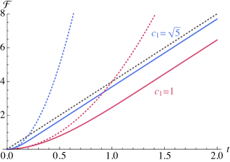
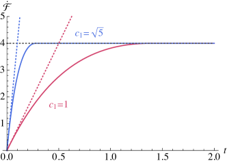
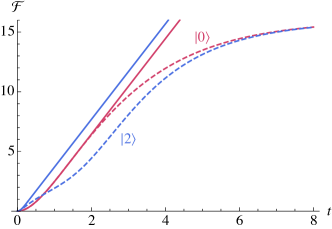
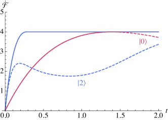
Figure 1: Top-left panel: Plots of $\mathcal{F}(t)$ bounds in the HLS case from Section II, compared to those from previous work. The solid curves correspond to the bound on $\mathcal{F}(t)$ from Eq. (31); the red curves take $c_{1}=1$, $c_{2}=1$ (all quantities are taken to be dimensionless), and the blue curves take $c_{1}=\sqrt{5}$, $c_{2}=1$. The gray dotted line shows the $\mathcal{F}(t)\leq 4c_{2}t$ bound from Demkowicz-Dobrzański et al. (2017); Zhou et al. (2018) (Eq. (26)), while the red and blue dotted curves correspond to the quadratic bounds from Eq. (33), for the appropriate $c_{1}$. Top-right panel: As per the top-left panel, but plotting $\dot{\mathcal{F}}(t)$ bounds. This illustrates how the large-$t$ scaling of our bounds is only affected by $c_{2}$, and not $c_{1}$. Bottom-left panel: Solid curves as in top row plots; dashed curves plot $\mathcal{F}(t)$ for different detection schemes with a damped harmonic oscillator probe, as considered in Section II.5 (taking $\gamma=1$ and $n_{T}=0$). The dashed red curve corresponds to preparing an oscillator in its ground state, and allowing it to evolve unimpeded under the influence of the linear forcing. This attains our $\mathcal{F}(t)$ bound (solid red curve) for $c_{1}=c_{2}=1$ at $t\leq t_{c}=2(c_{2}/c_{1}^{2})\ln 2\simeq 1.4$, but then asymptotes to a constant value of $\mathcal{F}(t)$. The blue dashed curve corresponds to preparing an oscillator in the $N=2$ Fock state, and allowing it to evolve. This has faster $\mathcal{F}(t)$ growth rate at small times, but that growth slows down for $t\gtrsim t_{c}=\frac{2\ln 2}{5}\simeq 0.3$. As well as representing the Eq. (31) bound with $c_{1}=1$, the solid red curve also corresponds to $\mathcal{F}(t)$ for a harmonic oscillator prepared in its ground state, but coupled to a continuum of ancillae for $t\geq t_{c}=2\ln 2$, to maintain the system at $\dot{\mathcal{F}}=4c_{2}$. Bottom-right panel: As per the bottom-left panel, but plotting $\dot{\mathcal{F}}(t)$.

In this subsection, we study the case where the probe system is a (weakly) damped harmonic oscillator, subject to some near-resonant forcing. This is a rather more complex and interesting example than the single spin from Eq. (2), and illustrates different points of theoretical and practical interest. Since an oscillator is an infinite-dimensional system, the methods of Demkowicz-Dobrzański et al. (2017); Zhou et al. (2018) do not apply directly. While one can sometimes consider restrictions to a finite-dimensional subspace—for instance, to states with occupation number $\leq N_{0}$ for some $N_{0}$—physical processes often generate evolution that cannot be contained within any finite-dimensional subspace (e.g., any continuous range of coherent state amplitudes). In addition, our methods allow us to treat time-dependent $H^{\prime}$, as we will further expand on in Section III. From an experimental perspective, many systems of interest, such as microwave, optical, or acoustic modes, are well-described by oscillators.

We will show that simple, physically relevant forms for $H$ are such that $H^{\prime}$ is in the Lindblad span (cf. Section II.4.1), so we can obtain an $\mathcal{F}$-independent bound on $\dot{\mathcal{F}}$ by choosing $G=0$ in Eq. (17). Moreover, this bound can be attained, for on-resonance forcings, by an oscillator prepared in any coherent state. However, non-classical states can lead to faster short-time QFI growth, as we will illustrate.

In the rotating wave approximation (RWA), the master equation for a harmonic oscillator interacting with a Markovian environment at temperature $T$ is Walls and Milburn (2008)

$$\dot{\rho} =-i[H,\rho]+\gamma(n_{T}+1)\left(a\rho a^{\dagger}-\frac{1}{2}\{a^{\dagger}a,\rho\}\right)$$

$$\quad+\gamma n_{T}\left(a^{\dagger}\rho a-\frac{1}{2}\{aa^{\dagger},\rho\}\right).$$ (39)

Here, $a^{\dagger}$ and $a$ are the oscillator’s creation and annihilation operators, $H$ is the RWA interaction Hamiltonian, $\gamma$ is the coupling to the Markovian bath (if the oscillator has no other influences acting on it, then $\gamma$ is its damping rate), and $n_{T}$ is the thermal occupation number corresponding to the temperature of the bath ($n_{T}=(e^{\omega/T}+1)^{-1}$, where $\omega$ is the resonant frequency of the oscillator). Thus, we have two Lindblad operators,

$$L_{1}=\sqrt{\gamma(n_{T}+1)}a,\quad L_{2}=\sqrt{\gamma n_{T}}a^{\dagger}.$$ (40)

The simplest kind of forcing we can consider is linear in the creation/annihilation operators and in $g$, so that

$$H^{\prime}=i\epsilon(t)a^{\dagger}+{\rm h.c.},$$ (41)

corresponding to a near-resonant force on the oscillator (with $\epsilon(t)$ representing the fiducial amplitude and phase of the forcing, and $g$ representing its relative amplitude). In this case, $H^{\prime}$ can be decomposed in the Lindblad span as in Eq. (25), but the decomposition is not unique. To obtain the best large-$\mathcal{F}$ bound from Eq. (17), we want to minimise $\sum_{j}\widetilde{A}_{j}^{\dagger}\widetilde{A}_{j}$, which is always a multiple of the identity in this case, since $\widetilde{\gamma}_{jk}=0$ for any such decomposition. To do so, we should choose $\widetilde{\beta}_{1}=\frac{i\epsilon}{\sqrt{\gamma}}\frac{\sqrt{n_{T}+1}}{2n_{T}+1}$ and $\widetilde{\beta}_{2}=\frac{\sqrt{n_{T}}}{2n_{T}+1}\frac{-i\epsilon^{*}}{\sqrt{\gamma}}$, giving $\sum_{j}\widetilde{A}_{j}^{\dagger}\widetilde{A}_{j}=\frac{|\epsilon|^{2}}{\gamma(2n_{T}+1)}I$. Note that if any of $\epsilon$, $n_{T}$, or $\gamma$ are time-dependent, then this quantity will be time-dependent.

On the other hand, the short-time QFI growth rate is determined by $\mathcal{F}_{H^{\prime}}$ (cf. Section II.3). From Fact 3, $\mathcal{F}_{H^{\prime}}\leq 4\operatorname{Var}(H^{\prime})$, with equality for pure states. This means that $\mathcal{F}_{H^{\prime}}$ is bounded by the fluctuations in the appropriate quadrature (for $\epsilon$ real, simply the momentum fluctuations of the oscillator). Since a coherent state is a minimum-uncertainty state, with equal uncertainties in all quadratures, these fluctuations can only be made large by putting the oscillator into a ‘non-classical’ state—that is, a state which is not a probability mixture of coherent states.

In the notation of Eq. (30), we have $c_{2}=\frac{|\epsilon|^{2}}{\gamma(2n_{T}+1)}$ and $c_{1}^{2}\leq 2|\epsilon|^{2}\sigma_{\widetilde{p}}^{2}$, where $\widetilde{p}\coloneqq\frac{1}{\sqrt{2}|\epsilon|}H^{\prime}$ is the appropriate quadrature operator, and $\sigma_{\widetilde{p}}^{2}\coloneqq\langle\widetilde{p}^{2}\rangle-\langle\widetilde{p}\rangle^{2}$ is its variance. If $c_{1}$ and $c_{2}$ are time-independent, then starting from $\mathcal{F}(t=0)=0$, Eq. (31) gives

$$\mathcal{F}(t)\leq\begin{dcases}\frac{8|\epsilon|^{2}}{\gamma_{T}^{2}\sigma_{\widetilde{p}}^{2}}\left(1-e^{-\gamma_{T}t\sigma_{\widetilde{p}}^{2}}\right)^{2}&\quad t\leq\frac{\ln 2}{\gamma_{T}\sigma_{\widetilde{p}}^{2}}\\ \frac{4|\epsilon|^{2}}{\gamma_{T}}t-\frac{2(\ln 4-1)|\epsilon|^{2}}{\gamma_{T}^{2}\sigma_{\widetilde{p}}^{2}}&\quad t\geq\frac{\ln 2}{\gamma_{T}\sigma_{\widetilde{p}}^{2}}\end{dcases}$$ (42)

where $\gamma_{T}\coloneqq\gamma(2n_{T}+1)$. If $c_{1}$ and $c_{2}$ vary with time, then we could integrate Eq. (30) to obtain analogous bounds.

The simplest situation for which we can analyse the actual behaviour of $\mathcal{F}(t)$ (as opposed to an upper bound) is when $H=gH^{\prime}$ and $n_{T}=0$. In this case, coherent states evolve to other coherent states, so if the oscillator starts in a coherent state, its state remains pure and coherent throughout Walls and Milburn (2008). The coherent state $|\alpha(t,g)\rangle$, with amplitude $\alpha(t,g)$, evolves as $\dot{\alpha}=g\epsilon-\frac{\gamma}{2}\alpha$. Consequently, if $\epsilon$ and $\gamma$ are time-independent, then

$$\alpha(t,g) =\frac{2g\epsilon}{\gamma}(1-e^{-\gamma t/2})+e^{-\gamma t/2}\alpha(t=0,g)$$

$$\eqqcolon g\alpha_{\epsilon}(t)+e^{-\gamma t/2}\alpha_{0}$$ (43)

To find $\mathcal{F}(t)$, we can use the fact that if $\rho(t,g)$ is pure for all $g$ (as is true here), then $\mathcal{L}=2\rho^{\prime}$. Consequently, writing $\rho=|\psi\rangle\langle\psi|$, we have $\mathcal{F}=4|\|\varphi_{\perp}\rangle\|^{2}$, where $|\varphi_{\perp}\rangle$ is the component of $\partial_{g}|\psi\rangle$ orthogonal to $|\psi\rangle$. To evaluate $|\varphi_{\perp}\rangle$, we note that $D(\beta)D(\delta)=e^{(\beta\delta^{*}-\beta^{*}\delta)/2}D(\beta+\delta)$ for any $\beta,\delta\in\mathbb{C}$, where $D$ is the displacement operator which generates coherent states, $D(\beta)=e^{\beta a^{\dagger}-\beta^{*}a}$. That is, $D(\beta)D(\delta)$ and $D(\beta+\delta)$ are equal, up to phase. Furthermore,

$$\partial_{g}D(g\alpha_{\epsilon})=\partial_{g}e^{g(\alpha_{\epsilon}a^{\dagger}-\alpha_{\epsilon}^{*}a)}=(\alpha_{\epsilon}a^{\dagger}-\alpha_{\epsilon}^{*}a)D(g\alpha_{\epsilon})$$ (44)

Consequently, if $\alpha_{0}$ is independent of $g$, then

$$|\varphi_{\perp}\rangle=e^{i\phi}D(e^{-\gamma t/2}\alpha_{0})(\alpha_{\epsilon}a^{\dagger}-\alpha_{\epsilon}^{*}a)D(g\alpha_{\epsilon})|0\rangle$$ (45)

for some $\phi\in\mathbb{R}$. Evaluating $\||\varphi_{\perp}\rangle\|^{2}$, we obtain

$$\mathcal{F}(t)=4|\alpha_{\epsilon}|^{2}=\frac{16|\epsilon|^{2}}{\gamma^{2}}(1-e^{-\gamma t/2})^{2}$$ (46)

for any $\alpha_{0}$. Comparing this to the $t\leq t_{c}=\ln 2/(\gamma\sigma_{\widetilde{p}}^{2})$ bound in Eq. (42), we see that they are equal for $\sigma_{\widetilde{p}}^{2}=\frac{1}{2}$, which is true for any coherent state. Hence, preparing the oscillator in a coherent state and letting it evolve unimpeded saturates the corresponding $\mathcal{F}(t)$ bound for $t\leq t_{c}$. At $t=t_{c}$, Eq. (46) attains the $\dot{\mathcal{F}}=4c_{2}=4|\epsilon|^{2}/\gamma$ bound from Eq. (30).

For an unperturbed oscillator, $\dot{\mathcal{F}}(t)$ starts to decrease for $t>t_{c}$; left to evolve by itself, the oscillator’s state would simply asymptote to $\alpha=2g\epsilon/\gamma$, so $\mathcal{F}$ would asymptote to $16|\epsilon|^{2}/\gamma^{2}$, and $\dot{\mathcal{F}}$ would tend towards zero. This is illustrated by the dashed red curves in the bottom row of Figure 1. To avoid this, we need to transfer some of the information in the state of the oscillator into ancillary degrees of freedom. The simplest way to achieve this is to couple the oscillator to a continuum of bosonic modes, such that energy loss into the modes acts, from the oscillator’s point of view, like an extra source of damping. For example, if we viewed the oscillator as a cavity mode, we could couple this mode to a waveguide. To maintain $\dot{\mathcal{F}}$ at the optimal value, it turns out that the extra damping rate should be the same as the Markovian damping rate $\gamma$, corresponding to critical coupling of the oscillator to the continuum, giving an effective damping rate of $2\gamma$.

If one switches on this continuum coupling at $t_{c}$, then it maintains the system at the $\dot{\mathcal{F}}=4|\epsilon|^{2}/\gamma$ limit, and so saturates the $\mathcal{F}(t)$ bound in Eq. (42) throughout. This means that we can attain the bound in Eq. (42) (with $\sigma_{\widetilde{p}}^{2}=1/2$), which corresponds to the solid red curves in Figure 1. Practically, of course, it may be simpler to couple the mode to the continuum from the beginning; in that case, $\dot{\mathcal{F}}$ asymptotes towards the $4|\epsilon|^{2}/\gamma$ limit over a few damping times.

If we allow the oscillator to be in a non-classical state, then the state-independent $\dot{\mathcal{F}}\leq{4|\epsilon|^{2}}/{\gamma_{T}}$ bound still applies, but $\dot{\mathcal{F}}$ can increase faster starting from zero. From Section II.3, the short-time growth rate of $\mathcal{F}$ is set by $\mathcal{F}_{H^{\prime}}(t=0)$, and $\mathcal{F}_{H^{\prime}}\leq\operatorname{Var}(H^{\prime})$ with equality for pure states, so we obtain faster growth by using states with larger $H^{\prime}$ fluctuations. This is illustrated by the dashed blue curves in the bottom panels of Figure 1, which correspond to preparing the oscillator in an $N=2$ Fock state.

Since large fluctuations require large energies, one question we can ask is how large $\mathcal{F}_{H^{\prime}}$ can be, given some bound on $\langle N\rangle$. Writing $\widetilde{x}\coloneqq\frac{1}{\sqrt{2}|\epsilon|}(\epsilon a^{\dagger}+{\rm h.c.})$ for the quadrature orthogonal to $\widetilde{p}$, we have the uncertainty principle relation $\sigma_{\widetilde{x}}^{2}\sigma_{\widetilde{p}}^{2}\geq 1/4$, as well as the relation ${\widetilde{x}}^{2}+{\widetilde{p}}^{2}=2N+1$, where $N$ is the oscillator’s number operator. Together, these imply that Lang and Caves (2013)

$$\sigma_{\widetilde{p}}^{2}\leq\frac{1}{2}+\langle N\rangle+\sqrt{\langle N\rangle(\langle N\rangle+1)}$$ (47)

This inequality is saturated iff the state is a minimum-uncertainty state with zero mean, i.e., a squeezed coherent state. (For comparison, the $N$th Fock state has $\sigma_{\widetilde{p}}^{2}=N+\frac{1}{2}$.) Hence, since $\operatorname{Var}(H^{\prime})=2|\epsilon|^{2}\sigma_{\widetilde{p}}^{2}$, the maximum $\mathcal{F}(t)$ at small $t$, for given $\langle N\rangle$, is attained by preparing the oscillator in a squeezed coherent state, with squeezing quadrature appropriate to the phase of the forcing (this is analogous to the conclusions in Lang and Caves (2013)). Since enhanced $\widetilde{p}$ fluctuations correspond to suppressed $\widetilde{x}$ fluctuations, and the forcing displaces the state in the $\widetilde{x}$ direction, this is intuitive from a quantum fluctuations viewpoint.

The bound in Eq. (47) illustrates that given constraints on our state, we can often obtain sensible results even for infinite-dimensional systems, without having to restrict to a finite-dimensional subspace (as done in e.g., Zhou et al. (2018)). Another example of this is the case of quadratic forcing, $H^{\prime}=\omega_{f}N$ (as can arise in e.g., optomechanical systems). Taking $n_{T}=0$ for simplicity, we have $\widetilde{\gamma}_{11}=\omega_{f}/\gamma$ (in the notation of Eq. (25)), so $\langle\widetilde{A}_{1}^{\dagger}\widetilde{A}_{1}\rangle={\omega_{f}^{2}}\langle N\rangle/\gamma$. So, if we restrict to $\langle N\rangle\leq\overline{N}$, then we can take $c_{2}={\omega_{f}^{2}}\overline{N}/\gamma$ and $c_{1}^{2}\leq 2|\epsilon|^{2}(\frac{1}{2}+\overline{N}+\sqrt{\overline{N}(\overline{N}+1)})$, and obtain the corresponding bounds using Eq. (31).

The linear ($H^{\prime}=i\epsilon a^{\dagger}+{\rm h.c.}$) and quadratic ($H^{\prime}\propto N$) forcings are simple, physically important examples which are in the Lindblad span. For $H^{\prime}$ other than linear combinations of these, we are in the HNLS case, so $\dot{\mathcal{F}}$ can in principle grow without bound. Examples include the ‘Kerr effect’ Hamiltonian $H^{\prime}\propto N^{2}$ considered in Zhou et al. (2018), or (for $n_{T}=0$) quadratic Hamiltonians of the form $H^{\prime}=fa^{2}+{\rm h.c.}$ The latter can arise from coupling to a signal oscillating at close to twice the natural frequency of the oscillator. Since this kind of forcing preserves the occupation number parity of the oscillator, whereas Lindblad jumps change it, schemes such as those based on ‘cat codes’ Cochrane et al. (1999) could be used to attain large $\dot{\mathcal{F}}$.

While the results in this subsection apply regardless of the $g$-independent dynamics of the system, they do assume that the oscillator is described by the master equation in Eq. (39). In particular, they rely on the assumption that the noise is Markovian. If the correlation time of the system-environment interaction is not small enough to be neglected, then techniques such as dynamic decoupling Viola and Lloyd (1998); Viola et al. (1999) can violate the above bounds.

III Sensitivity bandwidth

In Section II, we considered a Hamiltonian parameterised by a single unknown scalar parameter $g$. Apart from the value of $g$, we assumed that the form—in particular, the time dependence—of our Hamiltonian was known a priori. However, as discussed in the introduction, in many circumstances we are interested in a range of possible time dependences.

There are a number of ways to formalise this more general problem. We may view our task as simultaneously estimating a large number of parameters controlling the Hamiltonian, as in the ‘waveform estimation’ problem discussed in Tsang et al. (2011). Alternatively, we could attempt to estimate a single parameter, e.g., one controlling the overall strength of our signal, with other parameters viewed as ‘nuisance parameters’ Demkowicz-Dobrzański et al. (2020). The latter is the appropriate approach in e.g., axion dark matter detection, where we are interested in detecting the presence of a signal, and not in its detailed time dependence (at least for initial discovery purposes).

As a simple example, we will study the scenario of a scalar time dependence; that is, where the Hamiltonian has the form $H(t)=f(t,[g_{i}])\widetilde{H}+H_{c}$, where $[g_{i}]$ is some vector of scalar parameters, $f(t,[g_{i}])$ is a scalar function, $\widetilde{H}$ is a $t$- and $[g_{i}]$-independent operator, and $H_{c}$ is a $[g_{i}]$-independent operator. Examples of this form include oscillatory signals with known coupling type, but a priori unknown time dependence, as arise in searches for axion dark matter or gravitational waves.

III.1 Waveform estimation

We can consider a toy version of the waveform estimation problem by taking our signal to be stepwise constant. Specifically, suppose that the parameter $g_{i}$ controls the signal during the time interval $[t_{i},t_{i+1})$, so that $H=H_{c}+\sum_{i}g_{i}\mathbf{1}_{[t_{i},t_{i+1})}\widetilde{H}$. If we take the $g_{i}$ parameters to be independent, then we can simply consider independent single-parameter estimation problems on each time interval $[t_{i},t_{i+1})$; for each of these problems, the bounds we derived in Section II apply to the QFI $\mathcal{F}_{i}$ for each parameter $g_{i}$.

Now, suppose that we have some time-independent bound $\dot{\mathcal{F}}_{\rm max}$ on the QFI growth rate. As an example, if $\widetilde{H}$ is in the Lindblad span, then Eq. (30) gives such a bound if $c_{2}$ is time-independent. Then, over the total time $t_{\rm tot}\coloneqq\sum_{i}(t_{i+1}-t_{i})$, the sum of the individual QFIs $\mathcal{F}_{i}$ is bounded by $\sum_{i}\mathcal{F}_{i}\leq\dot{\mathcal{F}}_{\rm max}t_{\rm tot}$. The sum of the QFIs gives an upper bound for e.g., how well we can distinguish between two specific hypotheses for the vector $[g_{i}]$. Furthermore, suppose that we have a time-independent bound $\mathcal{F}_{\widetilde{H},\max}$ on $\mathcal{F}_{\widetilde{H}}$. Then, by setting $G=H^{\prime}$ in Eq. (17) and integrating from $\mathcal{F}_{i}=0$ at $t=t_{i}$, we have $\mathcal{F}_{i}(t)\leq\mathcal{F}_{\widetilde{H},\rm max}(t-t_{i})^{2}$ for $t\geq t_{i}$. Substituting this back into Eq. (17), we have $\dot{\mathcal{F}}_{i}\leq 2\mathcal{F}_{\widetilde{H},\rm max}(t-t_{i})$. Thus, the time taken to attain $\dot{\mathcal{F}}_{i}=\dot{\mathcal{F}}_{\rm max}$ is at least $t_{c}\sim\dot{\mathcal{F}}_{\rm max}/\mathcal{F}_{\widetilde{H},\max}$. We can make the constant factor more precise using the results from Sections II.4.1 and II.4.2; as discussed below Eq. (31), in some circumstances it will also be possible to parametrically tighten this bound.

Hence, if $|t_{i+1}-t_{i}|\lesssim t_{c}$ for every $i$, then $\sum_{i}\mathcal{F}_{i}\simeq\dot{\mathcal{F}}_{\rm max}t_{\rm tot}$ cannot be attained. Conversely, for the damped harmonic oscillator analysed in Section II.5, if we use the state-independent bound $\dot{\mathcal{F}}_{\rm max}=4|\epsilon|^{2}/\gamma$, then Eqs. (42) and (46) show that if $|t_{i+1}-t_{i}|\gtrsim t_{c}$, then we can approximately attain $\sum\mathcal{F}_{i}\simeq\dot{\mathcal{F}}_{\rm max}t_{\rm tot}$. Viewing the time-step widths as corresponding to the inverse bandwidth of our signal, the bandwidth $\Delta\omega$ over which we can attain $\sum\mathcal{F}_{i}\simeq\dot{\mathcal{F}}_{\rm max}t_{\rm tot}$ is $\Delta\omega\lesssim{\mathcal{F}_{\widetilde{H},\rm max}}/{\dot{\mathcal{F}}_{\max}}$.

This step-function analysis is obviously rather crude; we leave a more sophisticated analysis (along the lines of Tsang et al. (2011), which treats the noiseless case) to future work. However, it does illustrate the important point that even though the peak sensitivity to any given signal is bounded by $\dot{\mathcal{F}}_{\rm max}$, the sensitivity bandwidth is controlled by the finite-time QFI growth rate, and is bounded by $\mathcal{F}_{\widetilde{H},\rm max}/\dot{\mathcal{F}}_{\rm max}$. In the harmonic oscillator example, we can take $\dot{\mathcal{F}}_{\rm max}=4|\epsilon|^{2}/\gamma$, which is independent of the system’s state, and can be attained by an oscillator in its ground state—in that sense, there is no benefit to using ‘non-classical’ states. However, as shown in Section II.5, such states can enhance the short-time growth rate of $\mathcal{F}$, and consequently, the range of different time dependences we are sensitive to.

III.2 Nuisance parameters

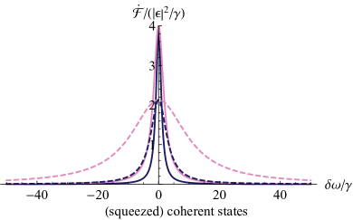
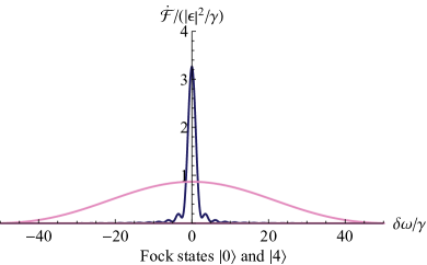
Figure 2: Plots of $\dot{\mathcal{F}}$ (at large times) for a damped harmonic oscillator, as a function of the detuning $\delta\omega$ of the signal frequency from the oscillator’s resonant frequency. The oscillator is assumed to be governed by the master equation in Eq. (39) (with $n_{T}=0$). Left panel: The blue curve corresponds to an oscillator that is critically coupled to ancillary degrees of freedom (e.g., a cavity mode coupled to a waveguide output), and initialised in its ground state. As discussed in Section II.5, this setup attains the $\dot{\mathcal{F}}\leq 4|\epsilon|^{2}/\gamma$ bound at large enough times, for a resonant forcing. The pink curve corresponds to an oscillator critically coupled to a source of squeezed vacuum, with squeezing parameter $G_{s}=4$. The dashed pink curve corresponds to the oscillator being overcoupled to the same squeezed state source by a factor $\sim 4G_{s}$, which decreases on-resonance sensitivity by a constant factor, but results in a sensitivity bandwidth $\sim G_{s}$ times larger than for preparation in the ground state (Section III.2). This is illustrated by the dashed blue curve, which corresponds to preparation in the ground state, overcoupled such that the on-resonance sensitivity matches that of the dashed pink curve. Right panel: Plot of the time-averaged rate of accumulation of (classical) Fisher information for a scheme in which the oscillator is prepared in a Fock state, and then measured in the Fock basis after evolving for a time $t_{1}$, as described in Section III.3. The blue curve corresponds to preparation in the ground state, followed by measurement at the time which optimises on-resonance sensitivity ($t_{1}\simeq 2.5/\gamma$), while the pink curve corresponds to preparation in the $N=4$ state, followed by measurement at the time which optimises on-resonance sensitivity ($t_{1}\simeq 0.12/\gamma$).

Estimating all of the parameters affecting a signal, as in waveform estimation, is at least as hard as estimating some parameters with others viewed as ‘nuisance parameters.’ Consequently, we expect similar conclusions about sensitivity bandwidth to apply to the nuisance parameter case. However, it is still useful to see explicitly how estimating a single parameter, in the large-$\mathcal{F}$ regime, is affected by nuisance parameters which control the time dependence of $H^{\prime}$, as we will analyse in this subsection. In particular, we will illustrate that, even after long times, the range of different signals for which near-peak sensitivity can be maintained is controlled by the short-time QFI growth rate.

Specifically, suppose that $H=H(t,g,h)$ depends on an additional parameter $h$. For a given value of $h$, the distinguishability of different $g$ values is set by the QFI with respect to $g$. We will investigate the range of different $h$ values over which the QFI growth rate can be close-to-optimal. This sets an upper bound on the range of $h$ for which a given measurement scheme can have near-optimal sensitivity to $g$, if the measurement scheme is chosen without knowing $h$.

For simplicity, we will suppose that at $g=0$, we have $\partial_{h}H=0$ (i.e., that $g=0$ corresponds to ‘no forcing’). Henceforth, we will write $\partial\equiv\partial_{h}$, and equalities holding at $g=0$ will be notated via $\overset{0}{=}$, e.g., $\partial H\overset{0}{=}0$. As an example, if $g$ corresponds to the overall strength of the forcing, and $h$ controls its precise form, then at $g=0$ the $h$ parameter should have no effect. We will assume that $\rho$ is $g$- and $h$- independent at some initial time $t_{0}$. Taking the derivative of the master equation (Eq. (1)) with respect to $g$, we have

$$\dot{\rho}^{\prime}=-i[H^{\prime},\rho]-i[H,\rho^{\prime}]+\sum_{j}\left(L_{j}\rho^{\prime}L_{j}^{\dagger}-\frac{1}{2}\{L_{j}^{\dagger}L_{j},\rho^{\prime}\}\right)$$ (48)

and then taking the derivative of this with respect to $h$,

$$\partial\dot{\rho}^{\prime}\overset{0}{=}-i[\partial H^{\prime},\rho]-i[H,\partial\rho^{\prime}]+\sum_{j}\left(L_{j}\partial\rho^{\prime}L_{j}^{\dagger}-\frac{1}{2}\{L_{j}^{\dagger}L_{j},\partial\rho^{\prime}\}\right)$$ (49)

since $\partial H\overset{0}{=}0$ and consequently $\partial\rho\overset{0}{=}0$. This has the same form as Eq. (48), which suggests that we can use the bounds derived in Section II, replacing $H^{\prime}$ with $\partial H^{\prime}$ and $\rho^{\prime}$ with $\partial\rho^{\prime}$. More precisely, consider the state $\sigma(t,g,h)$, defined via the master equation

$$\dot{\sigma}=-i[H^{(\sigma)},\sigma]+\sum_{j}\left(L_{j}\sigma L_{j}^{\dagger}-\frac{1}{2}\{L_{j}^{\dagger}L_{j},\sigma\}\right)$$ (50)

where $H^{(\sigma)}(t,g,h)\coloneqq H(t,g=0,h)+\partial H(t,g,h)$, along with the initial condition

$$\sigma(t=t_{0})=\rho(t=t_{0})$$ (51)

for all $g$ and $h$. Noting that $H^{(\sigma)}\overset{0}{=}H$, we see that $\sigma$ obeys the same master equation as $\rho$ at $g=0$, implying that $\sigma\overset{0}{=}\rho$ for all $t\geq t_{0}$. Moreover, we have

$$\dot{\sigma}^{\prime}\overset{0}{=}-i[\partial H^{\prime},\sigma]-i[H,\sigma^{\prime}]+\sum_{j}\left(L_{j}\sigma^{\prime}L_{j}^{\dagger}-\frac{1}{2}\{L_{j}^{\dagger}L_{j},\sigma^{\prime}\}\right)$$ (52)

so $\sigma^{\prime}$ obeys the same differential equation as $\partial\rho^{\prime}$ for $g=0$. From the initial condition, we have $\sigma^{\prime}(t=t_{0})=\partial\rho^{\prime}(t=t_{0})=0$, so it follows that $\sigma^{\prime}\overset{0}{=}\partial\rho^{\prime}$ for all $t\geq t_{0}$. Therefore, $\partial\mathcal{L}\overset{0}{=}\mathcal{L}^{(\sigma)}$ where $\mathcal{L}$ is the SLD for $\rho$ and $\mathcal{L}^{(\sigma)}$ is the SLD for $\sigma$ (cf. Eq. (3)). These identities will allow us to use the bounds in Section II, applied to $\mathcal{F}^{(\sigma)}\coloneqq\operatorname{tr}(\sigma(\mathcal{L}^{(\sigma)})^{2})$, to make statements about $\mathcal{F}=\operatorname{tr}(\rho\mathcal{L}^{2})$.

We now specialise to a scalar time dependence of the form $H=g(f_{0}(t)+hf_{1}(t))\widetilde{H}+H_{c}$, where $\widetilde{H}$ is independent of $t$, $g$, and $h$, and $H_{c}$ is independent of $g$ and $h$. Then, the basic quantities are linear in $h$, so we can write $H^{\prime}=H^{\prime}_{0}+h\partial H^{\prime}$, $\rho^{\prime}=\rho^{\prime}_{0}+h\partial\rho^{\prime}$ (from Eq. (48)), and $\mathcal{L}=\mathcal{L}_{0}+h\partial\mathcal{L}$ (since $\mathcal{L}$ is linear in $\rho^{\prime}$), where zero subscripts indicate the values at $h=0$. Hence, from Eq. (7), $\dot{\mathcal{F}}$ is quadratic in $h$, with the $h^{2}$ term given by

$$\partial^{2}\dot{\mathcal{F}}\overset{0}{=}2i\operatorname{tr}(\rho[\partial H^{\prime},\partial\mathcal{L}])-\sum_{j}\operatorname{tr}(\rho[\partial\mathcal{L},L_{j}]^{\dagger}[\partial\mathcal{L},L_{j}]).$$ (53)

Since $\partial\mathcal{L}\overset{0}{=}\mathcal{L}^{(\sigma)}$ and $\partial H^{\prime}=(H^{(\sigma)})^{\prime}$, we have $\partial^{2}\dot{\mathcal{F}}\overset{0}{=}\dot{\mathcal{F}}^{(\sigma)}$ by Eq. (7).

Supposing that $\widetilde{H}$ is in the Lindblad span, and we can bound $\dot{\mathcal{F}}$ as in Eq. (30), then the large-$\mathcal{F}$ bound will scale with $h$ as $\dot{\mathcal{F}}_{\rm max}\propto(f_{0}+hf_{1})^{2}$ (for any $t$). Consequently, we will suppose that $\dot{\mathcal{F}}\leq(f_{0}+hf_{1})^{2}\dot{\mathcal{F}}_{b}$ for some time-independent $\dot{\mathcal{F}}_{b}$. We are interested in quantifying the range of different time dependences for which we can (approximately) attain this bound, using the same detection system. To do this, we can assume that $\dot{\mathcal{F}}$ attains the bound for $h=0$, and ask what is required for $\dot{\mathcal{F}}$ at positive and negative $h$ values to also (almost) attain the bound. Equating the $h^{2}$ terms in $\dot{\mathcal{F}}$ and $\dot{\mathcal{F}}_{\rm max}$, we must have $\partial^{2}\dot{\mathcal{F}}\simeq f_{1}^{2}\dot{\mathcal{F}}_{b}$.

Since $\partial^{2}\dot{\mathcal{F}}\overset{0}{=}\dot{\mathcal{F}}^{(\sigma)}$, then if $f_{1}(t)=0$ for $t$ less than some time $t_{f}$, we can use the finite-time QFI bounds derived in Section II. Taking the simplest example of a step function time dependence, i.e., $f_{1}=\Theta(t-t_{f})$, we have from Eqs. (30) and (31) that the time taken to attain $\dot{\mathcal{F}}^{(\sigma)}\simeq f_{1}^{2}\dot{\mathcal{F}}_{b}$ at $g=0$ is at least $t_{c}\sim{\dot{\mathcal{F}}_{b}}/{\mathcal{F}_{\widetilde{H},\rm max}}$, where $\mathcal{F}_{\widetilde{H},\rm max}$ is a bound on $\mathcal{F}_{\widetilde{H}}$.

From the discussion below Eq. (17), to saturate the large-$\mathcal{F}$ bound $\dot{\mathcal{F}}_{\rm max}$, we need $[L_{j},\mathcal{L}]\sqrt{\rho}=2\widetilde{A}_{j}\sqrt{\rho}$ for all $j$. In our case, since $\widetilde{A}_{j}\propto(f_{0}+hf_{1})$, we need different values of $\mathcal{L}$ for different $h$ values, if $f_{1}\neq 0$. For the scenario where $f_{1}=0$ for $t<t_{f}$, but changes suddenly at $t_{f}$, $\dot{\mathcal{F}}_{\rm max}$ will also change suddenly (for non-zero $h$) but $\mathcal{L}$ will take some time to change, so the system will take some time to attain the new $\dot{\mathcal{F}}_{\rm max}$. This is what the analysis above quantifies.

As expected, $t_{c}$ is the same parametric timescale we found for waveform estimation. However, the interpretation is slightly different. For different values of $h$, the evolution of the state will be different, and in particular, the optimal measurement (with classical Fisher information equal to the QFI) may be different. Consequently, attaining $\dot{\mathcal{F}}$ close to the bound is necessary, but potentially not sufficient, for there to be a single measurement scheme with close-to-optimal sensitivity for a range of $h$ values. However, as demonstrated by e.g., the explicit prepare-measure-reset scheme discussed below (Section III.3), it is generally possible to obtain a sensitivity bandwidth scaling as $t_{c}^{-1}$, though the numerical prefactors may differ.

For simple systems, we can explicitly analyse both the QFI growth and the performance of specific measurement schemes. An example is the detection of a near-resonant force acting on a damped harmonic oscillator. As we found in Section II.5, the bound $\dot{\mathcal{F}}\leq 4|\epsilon|^{2}/\gamma$ can be attained by an oscillator in a coherent state, for an on-resonance forcing. However, as illustrated in the left-hand panel of Figure 2, the $\dot{\mathcal{F}}$ value obtained for forcings of different frequencies falls off quickly for detunings $\delta\omega\gtrsim\gamma$, for an oscillator in a coherent state. This fall-off can be reduced by using states with larger $\hat{x}$ fluctuations, such as squeezed coherent states. The figure shows that for squeezing parameter $G_{s}$, corresponding to fluctuations with variance $G_{s}$ times larger than that in a coherent state, the bandwidth over which the $\dot{\mathcal{F}}$ bound is attained (to ${\mathcal{O}}(1)$) is increased by a factor $\sim G_{s}$.

This behaviour, shown in the left-hand panel of Figure 2, corresponds to the QFI growth analysis in this subsection, and puts an upper bound on how well any given measurement scheme can do. By analysing specific measurement schemes, we can see that this scaling can be attained (again, to ${\mathcal{O}}(1)$). In the right-hand panel of Figure 2, we show the sensitivity of a prepare-measure-reset scheme as discussed in Section III.3 (using Fock states of the oscillator), illustrating how states with larger $H^{\prime}$ fluctuations can result in larger sensitivity bandwidths. In Malnou et al. (2019), the sensitivity of linear amplification schemes with squeezed coherent states is analysed, with analogous results.

In summary, the analysis in this section shows that the $\sim t_{c}^{-1}$ scaling for the sensitivity bandwidth is the best achievable (even when we do not need to determine the nuisance parameters), while the analyses in Section III.3 show that this scaling can be attained. Our analysis here was rather schematic (and it would be interesting to treat this more precisely) but captures the parametrics involved, showing how the range of different time dependences that we can be sensitive to is set by the finite-time QFI growth rate.

III.3 Frequent measurements

One way to increase our sensitivity bandwidth (potentially at the expense of peak sensitivity) is to use a prepare-measure-reset procedure: we sequentially prepare our probe system in some known starting state, allow it to evolve for some small time $t_{1}$, and then measure (before resetting). If our signal changes slowly compared to $t_{1}$, then it will be approximately constant over each prepare-measure-reset cycle, and we will have similar sensitivities to signals with different rates of change. Consequently, the sensitivity bandwidth will be at least $\sim 1/t_{1}$.

Since the QFI bounds the classical Fisher information from any measurement, the total information we can obtain is bounded by the sum of the QFIs from each cycle. Hence, the appropriate figure of merit is $\mathcal{F}(t_{1})/t_{1}$, where $\mathcal{F}(t_{1})$ is the QFI at each measurement time. This can be bounded using the techniques from Section II. In particular, if we can treat $H^{\prime}$ as constant over each cycle, then to obtain $\mathcal{F}(t_{1})/t_{1}\gtrsim\dot{\mathcal{F}}_{c}$, for some $\dot{\mathcal{F}}_{c}$, we need $t_{1}\gtrsim\dot{\mathcal{F}}_{c}/\mathcal{F}_{H^{\prime},\rm max}$, where $\mathcal{F}_{H^{\prime},\rm max}$ is a bound on $\mathcal{F}_{H^{\prime},\rm max}$. So, if $1/t_{1}$ sets the sensitivity bandwidth, then $\Delta\omega\lesssim\mathcal{F}_{H^{\prime},\rm max}/\dot{\mathcal{F}}_{c}$.

A practical example of this kind of prepare-measure-reset scheme is the proposal to use Fock states of cavity modes for axion dark matter detection Chou (2019); Dixit et al. (2021). If we prepare an oscillator in a Fock state $|n\rangle$, then in the presence of a small (linear) forcing, the rates of $|n\rangle\rightarrow|n+1\rangle$ and $|n\rangle\rightarrow|n-1\rangle$ transitions are $\propto n+1$ and $n$, respectively. Consequently, $\mathcal{F}$ initially increases faster with larger $n$. However, the rate of damping-induced $|n\rangle\rightarrow|n-1\rangle$ transitions is also $\propto n$, so the growth of $\mathcal{F}$ slows down over a timescale $\sim\gamma/n$. This corresponds to the fact that, for given $\gamma$, we cannot violate the $\dot{\mathcal{F}}\leq 4|\epsilon|^{2}/\gamma$ bound. However, the faster initial growth rate increases the sensitivity bandwidth; quantitatively, $\langle H^{\prime 2}\rangle\propto 2n+1$, and $\mathcal{F}\sim(8n+4)(\gamma t)^{2}$ for small $t$. These points are illustrated by the dashed blue curve in the bottom panels of Figure 1, which corresponds to preparing the oscillator in an $n=2$ Fock state.

Experimentally, one usually imagines measuring in the Fock basis. This would not be the optimal basis in which to measure if we knew the phase of our signal; however, it is a simple and phase-independent choice (and for many signals, such as virialised axion dark matter, the phase will be unknown). For Fock basis measurements, the time-averaged rate of Fisher information gain is smaller than the time-averaged QFI growth rate, but only by an order-1 factor. Similarly, prepare-measure-reset schemes have smaller time-averaged QFI growth rate than is possible with ‘steady-state’ schemes that do not involve resets (assuming equivalent mean occupation number), but this is again an order-1 loss. Overall, as illustrated in the right-hand panel of Figure 2, one can still use non-classical states to obtain an enhanced sensitivity bandwidth using a prepare-measure-reset scheme despite these issues.

While we have mostly discussed the bandwidth over which it is possible to achieve near-peak sensitivity, one is often interested in other figures of merit, such as some kind of frequency-averaged sensitivity. For example, if we are searching for a signal of definite but unknown frequency, then the appropriate quantity might be the time-averaged $\dot{\mathcal{F}}$, averaged over the relevant frequency range. For the prepare-measure-reset procedure above, this is bounded by $\sim\dot{\mathcal{F}}\times{\mathcal{F}_{H^{\prime}}}/{\dot{\mathcal{F}}}\sim\mathcal{F}_{H^{\prime}}$. We obtain parametrically the same result for steady-state schemes. These relationships are analogous to ‘Energetic Quantum Limits’ derived in the gravitational wave literature Braginsky (2000); Pang and Chen (2019), which relate the frequency-averaged sensitivity to the quantum fluctuations of an optical mode’s energy (since the energy is the appropriate interaction operator for a gravitational wave coupling).

IV Conclusions

In this paper, we explored the problem of Hamiltonian parameter estimation for quantum systems subject to Markovian noise. In particular, we derived an upper bound (Eq. (18)) on the rate of increase of the quantum Fisher information, in terms of the Lindblad operators and the parameter derivative $H^{\prime}$ of the Hamiltonian. This bound tightens previous bounds obtained in the case of time-independent $H^{\prime}$ for a finite-dimensional system Demkowicz-Dobrzański et al. (2017); Zhou et al. (2018), and also applies directly to more general situations, such as time-dependent master equations, and/or infinite-dimensional systems.

For time-dependent signals, we showed that the range of different frequencies to which a system can have close-to-peak sensitivity is set by the finite-time QFI growth rate, which is bounded by the quantum fluctuations of $H^{\prime}$. This is true even in the large-time, large-QFI regime, illustrating how our bounds can be useful beyond simply studying early-time QFI growth. While many previous studies have focused on how non-classical states can lead to higher sensitivities to specific signals, our analysis illustrates another way in which they can provide metrological advantage—by expanding the sensitivity bandwidth. This applies even in cases where such states cannot improve a system’s peak sensitivity, such as in the example we analysed of a damped harmonic oscillator with linear forcing.

While such behaviour has been noted for particular schemes, such as force detection with squeezed coherent states Malnou et al. (2019), we demonstrated that it applies more generally. It may be interesting to investigate sensitivity bandwidth expansion in gravitational wave detection schemes using our methods; while there have been general metrological analyses of interferometric gravitational wave detection in the presence of noise (in particular, photon loss) Demkowicz-Dobrzański et al. (2013), these have generally focused on the sensitivity to a specific signal.

As noted throughout Section II, our bounds can be attained asymptotically (in the large-time limit) using the error-correction methods of Zhou et al. (2018); Zhou and Jiang (2020) (at least for time-independent $H^{\prime}$). However, it is not clear whether they can always be attained at finite times by using appropriate ancilla-assisted schemes. While we showed that this was possible in some cases, such as the damped oscillator considered in Section II.5, we leave the general question to future work.

Another direction in which our results could be extended is by considering multi-parameter estimation problems. While Section III considered very simple examples of multi-parameter estimation problems, e.g., separate parameters controlling separate time intervals, more general scenarios (such as those analysed in Górecki et al. (2020)) could be investigated.

In addition to systems whose time evolution is well-described by a Lindblad master equation, our methods could similarly be applied to quantum channels that are equivalent to evolution over a finite time under some Lindblad master equation, even if that master equation does not describe the continuous-time evolution of the system. This may be useful in analysing the QFI for states obtained from discrete applications of quantum channels, as considered in e.g., Zhou and Jiang (2021).

Appendix A Differentiability of QFI wrt time

To derive the bounds in Section II, we assumed that it is always possible to find a Hermitian operator $\mathcal{L}(t,g)$ such that

$$\rho^{\prime}(t,g)=\frac{1}{2}(\rho(t,g)\mathcal{L}(t,g)+\mathcal{L}(t,g)\rho(t,g))$$ (54)

In this appendix, we show that for any $\rho$ obeying a Lindblad master equation in which the operators are differentiable with respect to $g$, we can always find such an $\mathcal{L}$. We also prove that if $\rho$ is an analytic function of $t$, then $\mathcal{L}$ is differentiable with respect to $t$, except possibly at a set of isolated times (for given $g$). We then show that $\mathcal{F}$ must be continuous even at these isolated times.

For a given $t$ and $g$, let $\rho=\sum_{j}p_{j}|j\rangle\langle j|$ be a spectral decomposition of $\rho$. Then, Eq. (54) implies that for all $j,k$,

$$\langle j|\rho^{\prime}|k\rangle=\frac{1}{2}(p_{j}+p_{k})\langle j|\mathcal{L}|k\rangle.$$ (55)

Hence, we set

$$\langle j|\mathcal{L}|k\rangle=\frac{2\langle j|\rho^{\prime}|k\rangle}{p_{j}+p_{k}}$$ (56)

for all $(j,k)$ such that $p_{j}+p_{k}\neq 0$, while for $(j,k)$ such that $p_{j}=p_{k}=0$, we choose any arbitrary values for $\langle j|\mathcal{L}|k\rangle$ (that are consistent with Hermiticity). Clearly, this $\mathcal{L}$ will satisfy Eq. (54) provided that $\langle j|\rho^{\prime}|k\rangle=0$ for all $(j,k)$ such that $p_{j}=p_{k}=0$. The following proposition shows that if this condition on $\rho^{\prime}$ is satisfied at some initial time, then it is satisfied at all subsequent times.

Proposition 1.

Suppose that for some $t_{0},t_{1}$ such that $t_{0}<t_{1}$, $\rho(t_{1},g)$ is obtained from $\rho(t_{0},g)$ via a quantum channel:

$$\rho(t_{1},g)=\sum_{m}M_{m}(g)\rho(t_{0},g)M_{m}^{\dagger}(g),$$ (57)

where the Kraus operators $M_{m}$ are differentiable with respect to $g$. For some fixed value of $g$, let $\rho(t_{0},g)=\sum_{j}p_{j}|j\rangle\langle j|$ and $\rho(t_{1},g)=\sum_{J}P_{J}|J\rangle\langle J|$ be spectral decompositions of $\rho(t_{0},g)$ and $\rho(t_{1},g)$. If $\langle j|\rho^{\prime}(t_{0},g)|k\rangle=0$ for all $(j,k)$ such that $p_{j}=p_{k}=0$, then $\langle J|\rho^{\prime}(t_{1},g)|K\rangle=0$ for all $(J,K)$ such that $P_{J}=P_{K}=0$.

Proof.

For clarity, we will denote $\rho_{0}\equiv\rho(t_{0},g)$ and $\rho_{1}\equiv\rho(t_{1},g)$, and omit the $t$ and $g$ arguments of all operators. First, observe that for any $J$ such that $P_{J}=0$,

$$0 =\langle J|\rho_{1}|J\rangle$$

$$=\sum_{m}\langle J|M_{m}\rho_{0}M_{m}^{\dagger}|J\rangle$$

$$=\sum_{j:p_{j}\neq 0}p_{j}\sum_{m}\left|\langle J|M_{m}|j\rangle\right|^{2}.$$ (58)

This implies that

$$\langle J|M_{m}|j\rangle=0$$ (59)

for all $m$ for any $(j,J)$ such that $p_{j}\neq 0$ and $P_{J}=0$.

Differentiating Eq. (57) with respect to $g$, we obtain

$$\langle J|\rho_{1}^{\prime}|K\rangle$$

$$=\langle J|\sum_{m}\Big{(}M_{m}^{\prime}\rho_{0}M_{m}^{\dagger}+M_{m}\rho_{0}M_{m}^{\prime\dagger}+M_{m}\rho_{0}^{\prime}M_{m}^{\dagger}\Big{)}|K\rangle$$

$$=\sum_{m}\Bigg{[}\sum_{j:p_{j}\neq 0}p_{j}\Big{(}\langle J|M_{m}^{\prime}|j\rangle\langle j|M_{m}^{\dagger}|K\rangle$$

$$\qquad\qquad\qquad\enspace+\langle J|M_{m}|j\rangle\langle j|M_{m}^{\prime\dagger}|K\rangle\Big{)}$$

$$\qquad\quad+\sum_{j,k}\langle J|M_{m}|j\rangle\langle j|\rho_{0}^{\prime}|k\rangle\langle k|M_{m}^{\dagger}|K\rangle\Bigg{]}.$$ (60)

Consider any $(J,K)$ such that $P_{J}=P_{K}=0$. Then, the first two terms in Eq. (60) vanish by the result expressed in Eq. (59). For the third term, if $(j,k)$ is such that $p_{j}=p_{k}=0$, then $\langle j|\rho_{0}^{\prime}|k\rangle=0$ by assumption; otherwise, at least one of $\langle J|M_{m}|j\rangle$ or $\langle k|M_{m}^{\dagger}|K\rangle$ is zero by Eq. (59). Thus, the third term also vanishes. Therefore, $\langle J|\rho_{1}^{\prime}|K\rangle=0$ as claimed.

∎

Evolution via a Lindblad master equation allows us to write $\rho(t_{1},g)$ as a quantum channel on $\rho(t_{0},g)$ for any $t_{1}>t_{0}$, fulfilling the assumption in Eq. (57) of Proposition 1. Consequently, if we can find $\mathcal{L}(t_{0},g)$ at some initial time $t_{0}$ (e.g., if we prepare our system in a $g$-independent state, so $\rho^{\prime}(t_{0},g)=0$ at the start time $t_{0}$), then we can always find $\mathcal{L}(t,g)$ satisfying Eq. (54) at all subsequent times $t$, using Eq. (56).

For our analyses in Section II, we also assumed that $\mathcal{L}$ is differentiable with respect to $t$, except at a (possibly empty) set of isolated times. Writing $\mathcal{L}=\sum_{j,k}\mathcal{L}_{jk}|j\rangle\langle k|$, a sufficient condition is that $\mathcal{L}_{jk},|j\rangle$ and $|k\rangle$ are differentiable with respect to $t$ for all $j,k$.

If we consider arbitrary quantum channels, then it is simple to write down a channel such that $\mathcal{L}$ is not differentiable with respect to $t$, so we need to impose more conditions. Here, we analyse, as an example, the simple case where $\rho(t,g)$ is an analytic function of $t$ (for each $g$); this often serves as a good model for physical systems (e.g., if $\rho$ arises from a master equation whose operators are analytic functions of $t$, as in Section II.5). In this case, the eigenvalues $p_{j}(t)$ and eigenstates $|j(t)\rangle$ can be chosen to be analytic functions of $t$ Kato (1995). Hence, it remains to show that $\mathcal{L}_{jk}$ is differentiable with respect to $t$.

For given $(j,k)$, at any $t$ such that $p_{j}+p_{k}\neq 0$, Eq. (56) is clearly differentiable, since the $p_{j}$ and $|j\rangle$ are differentiable. Moreover, by analyticity, the set of points with $p_{j}+p_{k}=0$ (for some given $g$) is either the entire $t$ range, or a set of isolated points. In the latter case, we can split our $\mathcal{L}$ evolution into differentiable segments between these points. If $\mathcal{F}$ is continuous at these points, then $\mathcal{F}(t)$ for all $t$ can be obtained by integrating $\dot{\mathcal{F}}$ in the segments between the points. To show that $\mathcal{F}$ is continuous, we prove a strengthened version of Proposition 1.

Proposition 2.

Suppose that for some $t_{0},t_{1}$ such that $t_{0}<t_{1}$, $\rho(t,g)$ is obtained from $\rho(t_{0},g)$ via a quantum channel, for all $t$ in a neighbourhood $I_{1}$ of $t_{1}$:

$$\rho(t,g)=\sum_{m}M_{m}(t,g)\rho(t_{0},g)M_{m}^{\dagger}(t,g),$$ (61)

where the Kraus operators $M_{m}(t,g)$ are differentiable with respect to $g$ and $M_{m}^{\prime}(t,g)$ are continuous in $t$. For some fixed value of $g$, let $\rho(t,g)=\sum_{j}p_{j}(t)|j(t)\rangle\langle j(t)|$ denote the spectral decomposition of $\rho(t,g)$ for $t\in I_{1}$. Assume that $\langle j(t_{0})|\rho^{\prime}(t_{0},g)|k(t_{0})\rangle=0$ for all $(j,k)$ such that $p_{j}(t_{0})=p_{k}(t_{0})=0$. If for some $(j,k)$, we have $p_{j}(t)+p_{k}(t)=\mathcal{O}(f(t-t_{1})^{2})$ (for $|t-t_{1}|$ small) for some function $f=o(1)$, then $\langle j(t)|\rho^{\prime}(t,g)|k(t)\rangle=\mathcal{O}(f(t-t_{1}))$.

Proof.

The proof is similar to that of Proposition 1. For convenience, we will sometimes omit the argument $g$, and we denote $\rho_{0}\equiv\rho(t_{0},g)$ and $(A)_{Jj}(t)\equiv\langle J(t)|A(t)|j(t_{0})\rangle$ for any operator $A$ and indices $J,j$ (ranging over the eigenbasis of $\rho$).

Using the same argument that led to Eq. (58), we have that for any $J$,

$$p_{J}(t)=\sum_{j:p_{j}(t_{0})\neq 0}p_{j}(t_{0})\sum_{m}\left|(M_{m})_{Jj}(t)\right|^{2}$$ (62)

for all $t\in I_{1}$. Since $p_{j}(t_{0})$ are non-negative constants independent of $t$, we see that if $p_{J}((t)=\mathcal{O}(f(t-t_{1})^{2})$, then

$$(M_{m})_{Jj}(t)=\mathcal{O}(f(t-t_{1}))$$ (63)

for all $j$ such that $p_{j}(t_{0})\neq 0$.

Also, it follows from $\sum_{m}M_{m}^{\dagger}M_{m}=I$ Nielsen and Chuang (2011) that $\sum_{m}\sum_{j}|(M_{m})_{Jj}(t)|^{2}=1$, so

$$|(M_{m})_{Jj}(t)|\leq 1$$ (64)

for all $m,J,j$.

Differentiating Eq. (61) with respect to $g$, we have for any $J,K$,

$$\langle J(t)|\rho^{\prime}(t,g)|K(t)\rangle$$

$$=\sum_{m}\Bigg{[}\sum_{j:p_{j}(t_{0})\neq 0}p_{j}\Big{(}(M_{m}^{\prime})_{Jj}(t)(M_{m}^{\dagger})_{jK}(t)$$

$$\qquad\qquad\qquad\enspace+(M_{m}|j\rangle)_{Jj}(M_{m}^{\prime\dagger})_{jK}(t)\Big{)}$$

$$\qquad\quad+\sum_{j,k}(M_{m})_{Jj}(t)\langle j(t_{0})|\rho_{0}^{\prime}|k(t_{0})\rangle(M_{m}^{\dagger})_{kK}(t)\Bigg{]}.$$ (65)

Since $M_{m}^{\prime}$ is continuous in $t$, $(M_{m}^{\prime})_{Jj}(t),(M_{m}^{\prime\dagger})_{jK}(t)=O(1)$ for $|t-t_{1}|$ small. Hence, for any $(J,K)$ such that $p_{J}(t)+p_{K}(t)=\mathcal{O}(f(t-t_{1})^{2})$, the first two terms in Eq. (65) are both $\mathcal{O}(f(t-t_{1}))$, by the result expressed in Eq. (63). As for the third term, if $(j,k)$ is such that $p_{j}(t_{0})=p_{k}(t_{0})=0$, then $\langle j(t)|\rho_{0}^{\prime}|k(t)\rangle=0$ by assumption; otherwise, at least one of $(M_{m})_{Jj}(t)$ and $(M_{m}^{\dagger})_{kK}(t)$ is $\mathcal{O}(f(t-t_{1}))$ by Eq. (63), and the other is $\mathcal{O}(1)$ by Eq. (64) (and $\langle j(t_{0})|\rho^{\prime}_{0}|k(t_{0})\rangle$ is independent of $t$).

∎

The QFI is given by

$$\mathcal{F}=\operatorname{tr}(\rho\mathcal{L}^{2})=2\sum_{\begin{subarray}{c}j,k:\\ p_{j}+p_{k}\neq 0\end{subarray}}\frac{|\langle j|\rho^{\prime}|k\rangle|^{2}}{p_{j}+p_{k}}$$ (66)

If the denominator $p_{j}(t)+p_{k}(t)={\mathcal{O}}(f(t-t_{1})^{2})$ for some $t_{1}$ and $(j,k)$, then Proposition 2 shows that the numerator $|\langle j(t)|\rho^{\prime}(t,g)|k(t)\rangle|^{2}={\mathcal{O}}(f(t-t_{1})^{2})$. Thus, since $p_{j},p_{k}$ and $\langle j|\rho^{\prime}|k\rangle$ are all analytic in $t$, the Taylor series of the numerator and denominator around $t=t_{1}$ have leading terms of the same order in $t-t_{1}$. As a result, any apparent singularities in the RHS terms of Eq. (66) are removable, so $\mathcal{F}$ is continuous in $t$.

The continuity of the QFI, with respect to different variables, has been investigated in a number of papers Augusiak et al. (2016); Šafránek (2017); Rezakhani et al. (2019); as far as we are aware, Proposition 2 constitutes a new contribution on this topic, which may be of independent interest.

Appendix B Properties of $\mathcal{F}_{A}$

In this appendix, we review some properties of the quantum Fisher information $\mathcal{F}_{A}$ with respect to a Hermitian operator $A$, defined by Eqs. (14) and (16). (Note from Eq. (16) that $\mathcal{F}_{A}$ also depends on the state $\rho$.)

Fact 1.

For any Hermitian operator $A$ and density operator $\rho$, there exists a Hermitian operator $\mathcal{L}_{A}$ satisfying Eq. (14).

Proof.

Let $\rho=\sum_{j}p_{j}|j\rangle\langle j|$ be a spectral decomposition of $\rho$. Then, set

$$\langle j|\mathcal{L}_{A}|k\rangle=\frac{2\langle j|i[\rho,A]|k\rangle}{p_{j}+p_{k}}$$ (67)

for all $(j,k)$ for which $p_{j}+p_{k}\neq 0$, while for $(j,k)$ such that $p_{j}=p_{k}=0$, choose any value for $\langle j|\mathcal{L}|k\rangle$ (consistent with Hermiticity). This satisfies Eq. (14) since $\langle j|i[\rho,A]|k\rangle=0$ for all $(j,k)$ such that $p_{j}=p_{k}=0$.

∎

Fact 2.

For any Hermitian operator $A$, density operator $\rho$, and $a,b\in\mathbb{R}$, we have

$$\mathcal{F}_{aA+bI}=a^{2}\mathcal{F}_{A}.$$ (68)

Proof.

From Eq. (67) in the proof of Fact 1, we can choose $\mathcal{L}_{aA+bI}=a\mathcal{L}_{A}$, so $\mathcal{F}_{aA+bI}=\operatorname{tr}(\rho\mathcal{L}_{aA+bI}^{2})=\operatorname{tr}(\rho(a\mathcal{L}_{A})^{2})=a^{2}\mathcal{F}_{A}$ by Eq. (16).

∎

Fact 3 (Tóth and Apellaniz (2014), Equations 60 and 61).

For any Hermitian operator $A$ and density operator $\rho$, we have

$$\mathcal{F}_{A}(\rho)\leq\operatorname{tr}(\rho A^{2})-\operatorname{tr}(\rho A)^{2}=\operatorname{Var}_{\rho}(A),$$

with equality if $\rho$ is pure.

Fact 4.

For any Hermitian operators $A,B$ and density operator $\rho$, we have

$$\mathcal{F}_{A+B}\leq\left(\sqrt{\mathcal{F}_{A}}+\sqrt{\mathcal{F}_{B}}\right)^{2},$$ (69)

with equality iff $\sqrt{\rho}\mathcal{L}_{A}=c\sqrt{\rho}\mathcal{L}_{B}$ for $c\geq 0$ or $\sqrt{\rho}\mathcal{L}_{B}=0$.

Proof.

Note that $\mathcal{F}_{A}=\|\sqrt{\rho}\mathcal{L}_{A}\|^{2}_{2}$, with $\|\cdot\|_{2}$ the Hilbert-Schmidt norm. From Eq. (67), $\mathcal{L}_{A+B}=\mathcal{L}_{A}+\mathcal{L}_{B}$. Hence,

$$\mathcal{F}_{A+B} =\|\sqrt{\rho}\mathcal{L}_{A+B}\|_{2}^{2}$$

$$=\|\sqrt{\rho}(\mathcal{L}_{A}+\mathcal{L}_{B})\|_{2}^{2}$$

$$\leq\Big{(}\|\sqrt{\rho}\mathcal{L}_{A}\|_{2}+\|\sqrt{\rho}\mathcal{L}_{B}\|_{2}\Big{)}^{2}$$

$$=\left(\sqrt{\mathcal{F}_{A}}+\sqrt{\mathcal{F}_{B}}\right)^{2},$$ (70)

and the triangle inequality used in the third line is saturated iff $\sqrt{\rho}\mathcal{L}_{A}=c\sqrt{\rho}\mathcal{L}_{B}$ for $c\geq 0$ or $\sqrt{\rho}\mathcal{L}_{B}=0$.

∎

Appendix C Details for Section II.4

In this appendix, we fill in some of the details for Section II.4. We start by reviewing the QFI calculations in Demkowicz-Dobrzański et al. (2017); Zhou et al. (2018), which lead to the bound in Eq. (26) for the time-independent, HLS case (Appendix C.1). We then show (Appendix C.2) that the best bound that can be obtained for the HNLS case using the methods in Demkowicz-Dobrzański et al. (2017); Zhou et al. (2018) is Eq. (33). Finally, we provide the technical details leading to our HNLS bound in Eq. (37) (Appendix C.3).

C.1 Review of previous results

The bounds on the QFI in Demkowicz-Dobrzański et al. (2017); Zhou et al. (2018), which apply in the case of time-independent $H^{\prime}$ and $L_{j}$, were derived from formulae for the QFI for $N$ identical operations Demkowicz-Dobrzański and Maccone (2014); Fujiwara and Imai (2008), taking the limit in which $N\to\infty$, so that the time interval $dt=t/N\to 0$ for each operation becomes correspondingly short. The form given in Zhou et al. (2018) (Demkowicz-Dobrzański et al. (2017) gives a similar expression) is

$$\mathcal{F}(t)\leq 4\frac{t}{dt}\|\alpha_{dt}\|+4\left(\frac{t}{dt}\right)^{2}\|\beta_{dt}\|\left(\|\beta_{dt}\|+2\sqrt{\|\alpha_{dt}\|}\right),$$ (71)

where

$$\alpha_{dt}\coloneqq\sum_{j}\Big{(}K^{\prime}_{j}-i\sum_{k}h_{jk}K_{k}\Big{)}^{\dagger}\Big{(}K^{\prime}_{j}-i\sum_{l}h_{jl}K_{l}\Big{)}$$ (72)

and

$$\beta_{dt}\coloneqq i\sum_{j}\Big{(}K^{\prime}_{j}-i\sum_{k}h_{jk}K_{k}\Big{)}^{\dagger}K_{j},$$ (73)

with $K_{0}=I-(igH^{\prime}+\frac{1}{2}\sum_{j\geq 1}L_{j}^{\dagger}L_{j})dt$ and $K_{j}=L_{j}\sqrt{dt}$ for $j\geq 1$ the Kraus operators describing the time evolution over each interval of length $dt$, and $h$ an arbitrary Hermitian matrix. The RHS of Eq. (71) can be minimised over the choice of $h$.

Write $X=X^{(0)}+X^{(1)}\sqrt{dt}+X^{(2)}dt+\dots$ as the expansion of any quantity $X$ in powers of $\sqrt{dt}$. To obtain a sensible bound from Eq. (71) in the $dt\rightarrow 0$ limit, we need that

$$\alpha_{dt}^{(0)}=\alpha_{dt}^{(1)}=0,$$

$$\beta_{dt}^{(0)}=\beta_{dt}^{(1)}=0.$$ (74)

Moreover, if $\beta_{dt}^{(2)}\neq 0$, then we need that $\alpha_{dt}^{(2)}=0$ for the $8t^{2}\|\beta_{dt}^{(2)}\|\sqrt{\|\alpha_{dt}\|}/dt$ term to not blow up.

As shown in Zhou et al. (2018), $\alpha_{dt}^{(0)}=0$ $\Leftrightarrow$ $h_{0j}^{(0)}=0\enspace\forall\,j$ $\Rightarrow$ $\alpha_{dt}^{(1)}=\beta_{dt}^{(0)}=0$, in which case $\beta_{dt}^{(1)}=0$ $\Leftrightarrow$ $-h_{00}^{(1)}=0$. Then, under these conditions, we have

$$\beta_{dt}^{(2)} =-H^{\prime}-h_{00}^{(2)}I$$

$$\quad-\sum_{j\geq 1}\left(h_{0j}^{(1)}L_{j}+h_{0j}^{(1)*}L_{j}^{\dagger}\right)-\sum_{j,k\geq 1}h_{jk}^{(0)}L_{j}^{\dagger}L_{k}.$$ (75)

We see that this has the form of Eq. (8) if one makes the notational substitutions

$$G\leftrightarrow-\beta^{(2)}_{dt},\quad\alpha\leftrightarrow-h_{00}^{(2)},$$ (76)

$$\beta_{j}\leftrightarrow-h_{j0}^{(1)},\quad\gamma_{jk}\leftrightarrow-h_{jk}^{(0)}.$$ (77)

It can also be checked that $\alpha_{dt}^{(2)}=\sum_{j}A_{j}^{\dagger}A_{j}$ when Eq. (74) is satsified, where $A_{j}$ is defined as in Eq. (10).

Zhou et al. (2018) uses Eq. (71) to derive a bound for the HLS case, where $\beta^{(2)}_{dt}$ can be set to $0$. They show that with this choice, Eq. (71) reduces in the $dt\to 0$ limit to Eq. (26), which is the bound we compare to in section II.4.1.

C.2 HNLS bound derived from Eq. (71)

We now show that the best possible bound given by Eq. (71) for the HNLS case has the form in Eq. (33). Since $H^{\prime}$ is not in the Lindblad span, $\beta^{(2)}_{dt}$ cannot be set to zero, so as noted above, we need to have $\alpha_{dt}^{(2)}=0$. This holds iff $A_{j}=0$ for all $j$, i.e., (in our notation)

$$\sum_{k}\gamma_{jk}L_{k}=-\beta_{j}I$$ (78)

by Eq. (10), which implies that for all $j$,

$$\sum_{k}\gamma_{jk}L_{k}=\sum_{k}\gamma_{jk}\langle\psi|L_{k}|\psi\rangle$$ (79)

for any $|\psi\rangle$. We then have, for arbitrary $|\psi\rangle$,

$$\sum_{j}(\beta_{j}^{*}L_{j}+\beta_{j}L_{j}^{\dagger})+\sum_{j,k}\gamma_{jk}L_{j}^{\dagger}L_{k}$$

$$\quad=\sum_{j,k}\gamma_{jk}L_{j}^{\dagger}L_{k}$$

$$\quad=\sum_{j}L_{j}^{\dagger}\sum_{k}\gamma_{jk}\langle\psi|L_{k}|\psi\rangle$$

$$\quad=\sum_{k}(-\beta_{k}^{*}I)\langle\psi|L_{k}|\psi\rangle,$$ (80)

using Eqs. (78) and (79) along with $\gamma_{jk}=\gamma_{kj}^{*}$. This shows that $\sum_{j}(\beta_{j}^{*}L_{j}+\beta_{j}L_{j}^{\dagger})+\sum_{j,k}\gamma_{jk}L_{j}^{\dagger}L_{k}$ is proportional to the identity. Therefore, from Eq. (8), $G$ must be of the form

$$G=H^{\prime}-\overline{\alpha}I$$ (81)

for some $\overline{\alpha}\in\mathbb{R}$. Eq. (33) then follows from Eq. (71) by noting that $G$ corresponds to $-\beta_{dt}^{(2)}$ (under the conditions in Eq. (74)) and taking the minimum over $\overline{\alpha}$.

C.3 HNLS bound derived from Eq. (17)

In Section II.4.2, we derived bounds on $\mathcal{F}(t)$ in the generic case where $H^{\prime}$ and $L_{j}$ are time-dependent, and $H^{\prime}$ may or may not be in the Lindblad span at different times. Assuming time-independent bounds $c_{0},c_{1},c_{2}$ on the relevant operators, with $c_{1}\geq c_{0}$ (cf. Section II.4.2), the bound for $t\geq t_{c}\coloneqq\frac{2c_{2}}{(c_{1}-c_{0})^{2}}\ln\left(\frac{2c_{1}}{c_{1}+c_{0}}\right)$ is given in Eq. (37) as $\mathcal{F}(t)\leq y(t-t_{c})^{2}$, where the function $y$ is defined as

$$y(t)\coloneqq\frac{c_{2}}{c_{0}}\left[-W_{-1}\Bigg{(}-\frac{1}{e}\left(\frac{c_{0}+c_{1}}{c_{1}-c_{0}}\right)\exp\left(-\frac{2c_{0}^{2}}{c_{2}}t-\frac{2c_{0}}{c_{1}-c_{0}}\right)\Bigg{)}-1\right]$$ (82)

with $W_{-1}$ the lower branch of the Lambert-W function Corless et al. (1996). From Chatzigeorgiou (2013), for any $u>0$,

$$1+\sqrt{2u}+\frac{2}{3}u\leq-W_{-1}(-e^{-1-u})\leq 1+\sqrt{2u}+u.$$ (83)

We can write $y(t)=\frac{c_{2}}{c_{0}}[-W_{-1}(-e^{-1-u(t)})-1]$ with

$$u(t)\coloneqq\frac{2c_{0}^{2}}{c_{2}}t+\frac{2c_{0}}{c_{1}-c_{0}}-\ln\left(\frac{c_{0}+c_{1}}{c_{1}-c_{0}}\right),$$ (84)

which is non-negative for all $t\geq 0$, since $c_{1}\geq c_{0}$ and $c_{2}\geq 0$. Thus, by Eq. (83)

$$\frac{c_{2}^{2}}{c_{0}^{2}}\left[\sqrt{2u(t)}+\frac{2}{3}u(t)\right]^{2}\leq y(t)^{2} \leq\frac{c_{2}^{2}}{c_{0}^{2}}\left[\sqrt{2u(t)}+u(t)\right]^{2},$$ (85)

so since $u(t)=2\frac{c_{0}^{2}}{c_{2}}t+{\mathcal{O}}(1)$,

$$y(t)^{2}=4c_{0}^{2}t^{2}\left(1+{\mathcal{O}}(t^{-1/2})\right)$$ (86)

for large $t$. We have $\mathcal{F}(t)\leq y(t-t_{c})^{2}$, so this leads to Eq. (38), confirming the expected scaling.

We can also derive a simpler but weaker bound than Eq. (37), by choosing $\delta(t)=1$ for all times $t$ in Eq. (35), rather than choosing the optimal $\delta$ at each $t$. In that case, we obtain $\dot{\mathcal{F}}\leq 4(c_{0}\sqrt{\mathcal{F}}+c_{2})$, giving (for $\mathcal{F}(t=0)=0$)

$$\mathcal{F}(t) \leq\frac{c_{2}^{2}}{c_{0}^{2}}\left[-W_{-1}\Bigg{(}-\frac{1}{e}\exp\left(-\frac{2c_{0}^{2}}{c_{2}}t\right)\Bigg{)}-1\right]^{2}$$

$$\leq 4c_{0}^{2}t^{2}\left(1+\frac{1}{c_{0}}\sqrt{\frac{c_{2}}{t}}\right)^{2}$$

$$=4c_{2}t+4t^{2}c_{0}\left(c_{0}+2\sqrt{\frac{c_{2}}{t}}\right).$$ (87)

Thus, we obtain a bound on $\mathcal{F}(t)$ that looks rather similar to Eq. (71); an important difference is that it still behaves sensibly if $c_{0}$ and $c_{2}$ (which are analogous to $\|\beta_{dt}^{(2)}\|$ and $\|\alpha_{dt}^{(2)}\|$ in the context of Eq. (71)) are both non-zero. Of course, Eq. (87) is looser than Eq. (37); while this looser bound has the correct large-$t$ scaling, it is not tight at small $t$ (unlike Eq. (37)).

Appendix D Lindblad parameter estimation

In the main text, we assumed that only the Hamiltonian depends on our parameter $g$. This is a good model for many signal detection problems, in which a small, effectively classical influence acts on the detection system. However, we may also be interested in determining properties of the system-environment coupling, such as the temperature of a thermal environment, or the strength of the coupling. This can be modelled by estimating a parameter controlling the Lindblad operators.

Hence, in this appendix, we consider the most general case where both the Hamiltonian $H$ and the Lindblad operators $L_{j}$ depend on $g$. By substituting Eq. (1) into the expression for $\dot{\mathcal{F}}$ given in Eq. (6) and simplifying using Eq. (3), we obtain

$$\dot{\mathcal{F}} =2i\operatorname{tr}\left(\rho[H^{\prime},\mathcal{L}]\right)-\sum_{j}\operatorname{tr}\left(\rho[L_{j},\mathcal{L}]^{\dagger}[L_{j},\mathcal{L}]\right)$$

$$-2\sum_{j}\mathrm{Re}\left\{\operatorname{tr}\left(\rho\big{(}L_{j}^{\prime\dagger}[L_{j},\mathcal{L}]+L_{j}^{\dagger}[L_{j}^{\prime},\mathcal{L}]\big{)}\right)\right\}.$$ (88)

If we allow ourselves complete freedom to choose the Lindblad operators, it is easy to see that, even if $H^{\prime}=0$ here, we can obtain similarly complicated behaviour to the $g$-dependent $H$ case considered in the main text. In particular, suppose that we have one Lindblad operator $L_{1}$ and that at some $g=g_{0}$, we have $L_{1}=I$ and $L_{1}^{\prime\dagger}=iG$ for some Hermitian operator $G$. Then, the third term in Eq. (88) is equal to $2i\operatorname{tr}(\rho[G,\mathcal{L}])$, so $\dot{\mathcal{F}}$ would have the same form as our expression in Eq. (7) for the case of $g$-independent Lindblad operators, except with $H^{\prime}$ replaced by $H^{\prime}+G$. Consequently, for different choices of $G$, we can obtain all of the different behaviours studied in the main text. In particular, if $H^{\prime}+G$ is not in the Lindblad span, then $\dot{\mathcal{F}}$ can be arbitrarily large, for appropriate $\rho$ and $\mathcal{L}$ (corresponding to $\mathcal{F}$ being able to grow faster than linearly, as in the HNLS case).

This $L_{1}=I$ example is somewhat artificial, since a Lindblad operator that is proportional to the identity has no effect on the master equation. In some sense, the behaviour described above arises from a non-canonical choice of Lindblad operators. However, we can show that even for a canonical parameterisation of the Lindblad terms, similar behaviour can still arise (in particular, $\dot{\mathcal{F}}$ can still become arbitrarily large).

A canonical way of writing the master equation for finite-dimensional systems is

$$\dot{\rho}=-i[H,\rho]+\sum_{k,l}h_{kl}\Big{(}M_{k}\rho M_{l}^{\dagger}-\frac{1}{2}\left\{M_{l}^{\dagger}M_{k},\rho\right\}\Big{)},$$ (89)

where $h$ is a positive semidefinite matrix and $\{M_{k}\}_{k}$ is a fixed orthonormal basis for traceless operators. This is canonical in the sense that different choices of $h$ correspond to physically different master equations, whereas different choices of Lindblad operators $\{L_{j}\}_{j}$ in Eq. (1) can give rise to the same master equation. To arrive at this form, one takes each Lindblad operator $L_{j}$ in Eq. (1) to be traceless wlog (modifying $H$ if necessary) and decomposes it in the basis $\{M_{k}\}_{k}$.

Substituting Eq. (89) into Eq. (6) gives

$$\dot{\mathcal{F}} =2i\operatorname{tr}(\rho[H^{\prime},\mathcal{L}])-\sum_{k,l}h_{kl}\operatorname{tr}\left(\rho[M_{l},\mathcal{L}]^{\dagger}[M_{k},\mathcal{L}]\right)$$

$$-2\sum_{k,l}\mathrm{Re}\Big{\{}h_{kl}^{\prime}\operatorname{tr}\left(\rho M_{l}^{\dagger}[M_{k},\mathcal{L}]\right)\Big{\}}.$$ (90)

Since $h$ is positive semidefinite, we can write $h=s^{2}$ for some Hermitian matrix $s$, and we take $s$ to be differentiable with respect to $g$. Then,

$$-2\sum_{k,l}\mathrm{Re}\Big{\{}h_{kl}^{\prime}\operatorname{tr}\left(\rho M_{l}^{\dagger}[M_{k},\mathcal{L}]\right)\Big{\}}$$

$$=-2\sum_{j}\mathrm{Re}\Bigg{\{}\operatorname{tr}\Bigg{(}\rho\Big{(}\sum_{l}s_{lj}^{\prime}M_{l}\Big{)}^{\dagger}\Big{[}\sum_{k}s_{kj}M_{k},\mathcal{L}\Big{]}\Bigg{)}\Bigg{\}}$$

$$\quad\,-2\sum_{j}\mathrm{Re}\Bigg{\{}\operatorname{tr}\Bigg{(}\rho\Big{(}\sum_{l}s_{lj}M_{l}\Big{)}^{\dagger}\Big{[}\sum_{k}s_{kj}^{\prime}M_{k},\mathcal{L}\Big{]}\Bigg{)}\Bigg{\}}.$$ (91)

Noting that $\{\sum_{k}s_{kj}M_{k}\}_{j}$ is a valid set of Lindblad operators for Eq. (89), the first term of the RHS of Eq. (91) can be combined with the first two terms in Eq. (90), and then the resulting expression can be upper-bounded using a similar argument as that leading to Eq. (13) in the main text. In particular, if $H^{\prime}$ is in the Lindblad span, then the resulting bound is $\mathcal{L}$-independent. However, the second term in Eq. (91) cannot always be bounded in this way. Specifically, if $s$ is singular, and $s^{\prime}$ does not map the kernel of $s$ to itself, then for some $\rho$, we can make $\dot{\mathcal{F}}$ arbitrarily large by choosing $\mathcal{L}$ appropriately.

As a simple example, consider a two-level system, with a single Lindblad operator $L_{1}(g)=\sqrt{\gamma}(\cos g\,\sigma_{z}+\sin g\,\sigma_{y})$ (with $\gamma>0$), so that $g$ parameterizes the ‘direction’ of the dephasing on the Bloch sphere. At $g=0$,

$$\dot{\mathcal{F}} =2i\operatorname{tr}(\rho[H^{\prime},\mathcal{L}])+2\gamma\operatorname{Re}\operatorname{tr}(\rho[\sigma_{z},\mathcal{L}]\sigma_{y}+[\sigma_{y},\mathcal{L}]\sigma_{z})$$

$$-\gamma\operatorname{tr}(\rho[\sigma_{z},\mathcal{L}]^{\dagger}[\sigma_{z},\mathcal{L}]),$$ (92)

so if we have $\mathcal{L}=\alpha I+\beta\sigma_{z}$ for some $\alpha,\beta\in\mathbb{R}$, then $\dot{\mathcal{F}}=2\beta(i\operatorname{tr}(\rho[H^{\prime},\sigma_{z}])+2\gamma\operatorname{tr}(\rho\sigma_{y}))$. Consequently, even if $H^{\prime}$ is in the Lindblad span (so that $[H^{\prime},\sigma_{z}]=0$), we can have arbitrarily large $\dot{\mathcal{F}}$ if $\operatorname{tr}(\rho\sigma_{y})\neq 0$.

However, for more restricted forms of Lindblad parameter dependence, there do exist $\mathcal{L}$-independent bounds on $\dot{\mathcal{F}}$. In particular, if $g$ only affects the magnitude of the Lindblad operators, in the sense that $L_{j}=f_{j}(g)\hat{L}_{j}$ for some constant operators $\hat{L}_{j}$, with $f_{j}$ real wlog, then from Eq. (88), we have (for $H^{\prime}=0$),

$$\dot{\mathcal{F}} =-4\sum_{j}\mathrm{Re}\left\{\operatorname{tr}\left(f_{j}f_{j}^{\prime}\operatorname{tr}\big{(}\rho\hat{L}_{j}^{\dagger}[\hat{L}_{j},\mathcal{L}]\big{)}\right)\right\}$$

$$\quad-\sum_{j}f_{j}^{2}\operatorname{tr}\big{(}\rho[\hat{L}_{j}^{\dagger},\mathcal{L}]^{\dagger}[\hat{L}_{j},\mathcal{L}]\big{)}$$ (93)

$$\leq 4\sum_{j}\Bigg{(}|f_{j}^{\prime}|\sqrt{\operatorname{tr}(\rho\hat{L}_{j}^{\dagger}\hat{L}_{j})}\sqrt{f_{j}^{2}\operatorname{tr}(\rho[\hat{L}_{j},\mathcal{L}]^{\dagger}[\hat{L}_{j},\mathcal{L}])}$$

$$\quad-\frac{1}{4}f_{j}^{2}\operatorname{tr}(\rho[\hat{L}_{j},\mathcal{L}]^{\dagger}[\hat{L}_{j},\mathcal{L}])\Bigg{)}$$ (94)

$$\leq 4\sum_{j}(f_{j}^{\prime})^{2}\operatorname{tr}\left(\rho\hat{L}_{j}^{\dagger}\hat{L}_{j}\right)$$ (95)

by the same logic as that leading to Eq. (13) (non-zero $H^{\prime}$ can be handled straightforwardly via a very similar calculation). This illustrates an important difference from the Hamiltonian parameter estimation case studied in the main text, where we found that even if $H^{\prime}\propto H$, it is not necessarily in the Lindblad span, so there may not be a $\mathcal{L}$-independent bound on $\dot{\mathcal{F}}$. In contrast, if $L_{j}^{\prime}\propto L_{j}$, then Eq. (95) gives such a $\mathcal{L}$-independent bound. Thus, for estimating e.g., the strength of a specific coupling to the environment, or the temperature of a thermal bath [cf. Eq. (39)], $\mathcal{F}$ can grow at most linearly at large times (given a time-independent bound on $\langle\hat{L}_{j}^{\dagger}\hat{L}_{j}\rangle$).

Moreover, unlike in Hamiltonian parameter estimation, for which $\mathcal{F}\sim t^{2}$ at small $t$ if we start from $\mathcal{F}(t=0)=0$ (Section II.3), for master equations with $g$-dependent Lindblads, it is possible for $\dot{\mathcal{F}}$ to be nonzero even initially. In some circumstances, we can attain the bound from Eq. (95) immediately. For example, suppose that we have a single Lindblad operator $L_{1}$, with $g$-dependent magnitude. Then, if we start in a pure state $|\psi\rangle$, and $L_{1}|\psi\rangle\perp|\psi\rangle$, the inital value of $\dot{\mathcal{F}}$ saturates Eq. (95). As a specific case, we can consider a damped harmonic oscillator, starting in a Fock state $|n\rangle$, with $L_{1}=g\sqrt{\gamma}a$, so $L_{1}|n\rangle\propto|n-1\rangle$. Since the rate of damping-induced transitions is immediately non-zero (and only decreases with time), to determine the strength of the damping, we cannot do better than checking for decays over many short time periods (with intermediate resets). Since the environment is taken to be Markovian, with vanishing coherence time, there is no quantum Zeno effect, and we cannot enhance the damping rate by building up correlations with the detector system.

Therefore, in circumstances like these, the parameter estimation story is considerably less complicated than for Hamiltonian parameter estimation. Even though it is possible in principle for $g$-dependent Lindblad operators to yield more complex behaviour—for instance, as in the $g$-dependent ‘dephasing direction’ example (Eq. (D)) discussed above—this does not seem to commonly arise in cases of physical interest.

References

- Saulson (1994) P. R. Saulson, Fundamentals of Interferometric Gravitational Wave Detectors (WORLD SCIENTIFIC, 1994).
- Giovannetti et al. (2011) V. Giovannetti, S. Lloyd, and L. Maccone, Nature Photonics 5, 222 (2011).
- Miao et al. (2017) H. Miao, R. X. Adhikari, Y. Ma, B. Pang, and Y. Chen, Phys. Rev. Lett. 119, 050801 (2017), arXiv:1608.00766 [quant-ph] .
- Pang and Chen (2019) B. Pang and Y. Chen, Phys. Rev. D 99, 124016 (2019), arXiv:1903.09378 [quant-ph] .
- Lasenby (2021) R. Lasenby, Physical Review D 103 (2021), 10.1103/physrevd.103.075007.
- Wiseman and Milburn (2009) H. M. Wiseman and G. J. Milburn, Quantum Measurement and Control (Cambridge University Press, 2009).
- Sekatski et al. (2017) P. Sekatski, M. Skotiniotis, J. Kołodyński, and W. Dür, Quantum 1, 27 (2017).
- Demkowicz-Dobrzański et al. (2017) R. Demkowicz-Dobrzański, J. Czajkowski, and P. Sekatski, Physical Review X 7 (2017), 10.1103/physrevx.7.041009.
- Zhou et al. (2018) S. Zhou, M. Zhang, J. Preskill, and L. Jiang, Nature Communications 9 (2018), 10.1038/s41467-017-02510-3.
- Zhou and Jiang (2020) S. Zhou and L. Jiang, Physical Review Research 2 (2020), 10.1103/physrevresearch.2.013235.
- Graham et al. (2015) P. W. Graham, I. G. Irastorza, S. K. Lamoreaux, A. Lindner, and K. A. van Bibber, Annual Review of Nuclear and Particle Science 65, 485 (2015).
- Lasky (2015) P. D. Lasky, Publications of the Astronomical Society of Australia 32 (2015), 10.1017/pasa.2015.35.
- Malnou et al. (2019) M. Malnou, D. Palken, B. Brubaker, L. R. Vale, G. C. Hilton, and K. Lehnert, Physical Review X 9 (2019), 10.1103/physrevx.9.021023.
- Nielsen and Chuang (2011) M. A. Nielsen and I. L. Chuang, Quantum Computation and Quantum Information: 10th Anniversary Edition, 10th ed. (Cambridge University Press, USA, 2011).
- Hotta et al. (2005) M. Hotta, T. Karasawa, and M. Ozawa, Physical Review A 72 (2005), 10.1103/physreva.72.052334.
- Hotta et al. (2006) M. Hotta, T. Karasawa, and M. Ozawa, Journal of Physics A: Mathematical and General 39, 14465 (2006).
- Kołodyński and Demkowicz-Dobrzański (2013) J. Kołodyński and R. Demkowicz-Dobrzański, New Journal of Physics 15, 073043 (2013).
- Takeoka and Wilde (2016) M. Takeoka and M. M. Wilde, “Optimal estimation and discrimination of excess noise in thermal and amplifier channels,” (2016), arXiv:1611.09165 [quant-ph] .
- Pirandola and Lupo (2017) S. Pirandola and C. Lupo, Physical Review Letters 118 (2017), 10.1103/physrevlett.118.100502.
- Braunstein and Caves (1994) S. L. Braunstein and C. M. Caves, Physical Review Letters 72, 3439 (1994).
- Lu et al. (2010) X.-M. Lu, X. Wang, and C. P. Sun, Physical Review A 82 (2010), 10.1103/physreva.82.042103.
- Tóth and Apellaniz (2014) G. Tóth and I. Apellaniz, Journal of Physics A: Mathematical and Theoretical 47, 424006 (2014).
- Tsang et al. (2011) M. Tsang, H. M. Wiseman, and C. M. Caves, Physical Review Letters 106 (2011), 10.1103/physrevlett.106.090401.
- Demkowicz-Dobrzański and Maccone (2014) R. Demkowicz-Dobrzański and L. Maccone, Physical Review Letters 113 (2014), 10.1103/physrevlett.113.250801.
- Fujiwara and Imai (2008) A. Fujiwara and H. Imai, Journal of Physics A: Mathematical and Theoretical 41, 255304 (2008).
- Zhou (2021) S. Zhou, Error-Corrected Quantum Metrology, Ph.D. thesis (2021).
- Walls and Milburn (2008) D. Walls and G. J. Milburn, eds., Quantum Optics (Springer Berlin Heidelberg, 2008).
- Lang and Caves (2013) M. D. Lang and C. M. Caves, Physical Review Letters 111 (2013), 10.1103/physrevlett.111.173601.
- Cochrane et al. (1999) P. T. Cochrane, G. J. Milburn, and W. J. Munro, Physical Review A 59, 2631 (1999).
- Viola and Lloyd (1998) L. Viola and S. Lloyd, Physical Review A 58, 2733 (1998).
- Viola et al. (1999) L. Viola, E. Knill, and S. Lloyd, Physical Review Letters 82, 2417 (1999).
- Demkowicz-Dobrzański et al. (2020) R. Demkowicz-Dobrzański, W. Górecki, and M. Guţă, Journal of Physics A: Mathematical and Theoretical 53, 363001 (2020).
- Chou (2019) A. S. Chou, in Astrophysics and Space Science Proceedings (Springer International Publishing, 2019) pp. 41–48.
- Dixit et al. (2021) A. V. Dixit, S. Chakram, K. He, A. Agrawal, R. K. Naik, D. I. Schuster, and A. Chou, Phys. Rev. Lett. 126, 141302 (2021), arXiv:2008.12231 [hep-ex] .
- Braginsky (2000) V. B. Braginsky, in AIP Conference Proceedings (AIP, 2000).
- Demkowicz-Dobrzański et al. (2013) R. Demkowicz-Dobrzański, K. Banaszek, and R. Schnabel, Physical Review A 88 (2013), 10.1103/physreva.88.041802.
- Górecki et al. (2020) W. Górecki, S. Zhou, L. Jiang, and R. Demkowicz-Dobrzański, Quantum 4, 288 (2020).
- Zhou and Jiang (2021) S. Zhou and L. Jiang, PRX Quantum 2 (2021), 10.1103/prxquantum.2.010343.
- Kato (1995) T. Kato, Perturbation Theory for Linear Operators (Springer Berlin Heidelberg, 1995).
- Augusiak et al. (2016) R. Augusiak, J. Kołodyński, A. Streltsov, M. N. Bera, A. Acín, and M. Lewenstein, Physical Review A 94 (2016), 10.1103/physreva.94.012339.
- Šafránek (2017) D. Šafránek, Physical Review A 95 (2017), 10.1103/physreva.95.052320.
- Rezakhani et al. (2019) A. T. Rezakhani, M. Hassani, and S. Alipour, Physical Review A 100 (2019), 10.1103/physreva.100.032317.
- Corless et al. (1996) R. M. Corless, G. H. Gonnet, D. E. G. Hare, D. J. Jeffrey, and D. E. Knuth, Advances in Computational Mathematics 5, 329 (1996).
- Chatzigeorgiou (2013) I. Chatzigeorgiou, IEEE Communications Letters 17, 1505 (2013).