Multi-domain semantic segmentation with overlapping labels

Abstract

Deep supervised models have an unprecedented capacity to absorb large quantities of training data. Hence, training on many datasets becomes a method of choice towards graceful degradation in unusual scenes. Unfortunately, different datasets often use incompatible labels. For instance, the Cityscapes road class subsumes all driving surfaces, while Vistas defines separate classes for road markings, manholes etc. We address this challenge by proposing a principled method for seamless learning on datasets with overlapping classes based on partial labels and probabilistic loss. Our method achieves competitive within-dataset and cross-dataset generalization, as well as ability to learn visual concepts which are not separately labeled in any of the training datasets. Experiments reveal competitive or state-of-the-art performance on two multi-domain dataset collections and on the WildDash 2 benchmark.

1 Introduction

Large realistic datasets [17, 5, 21, 41] have immensely contributed to development of dense prediction models. The reported accuracy grew rapidly over the last five years so that some of these datasets appear solved today. Unfortunately, the learned models often perform poorly in the wild [36]. Consequently, a desire emerged to measure the model performance by evaluating on multiple datasets from several domains [16, 40, 15], akin to combined events in athletics. The most straightforward approach towards that goal is simultaneous training on many datasets. Such training is likely to yield outstanding resilience due to extremely large capacity of convolutional models [37, 31].

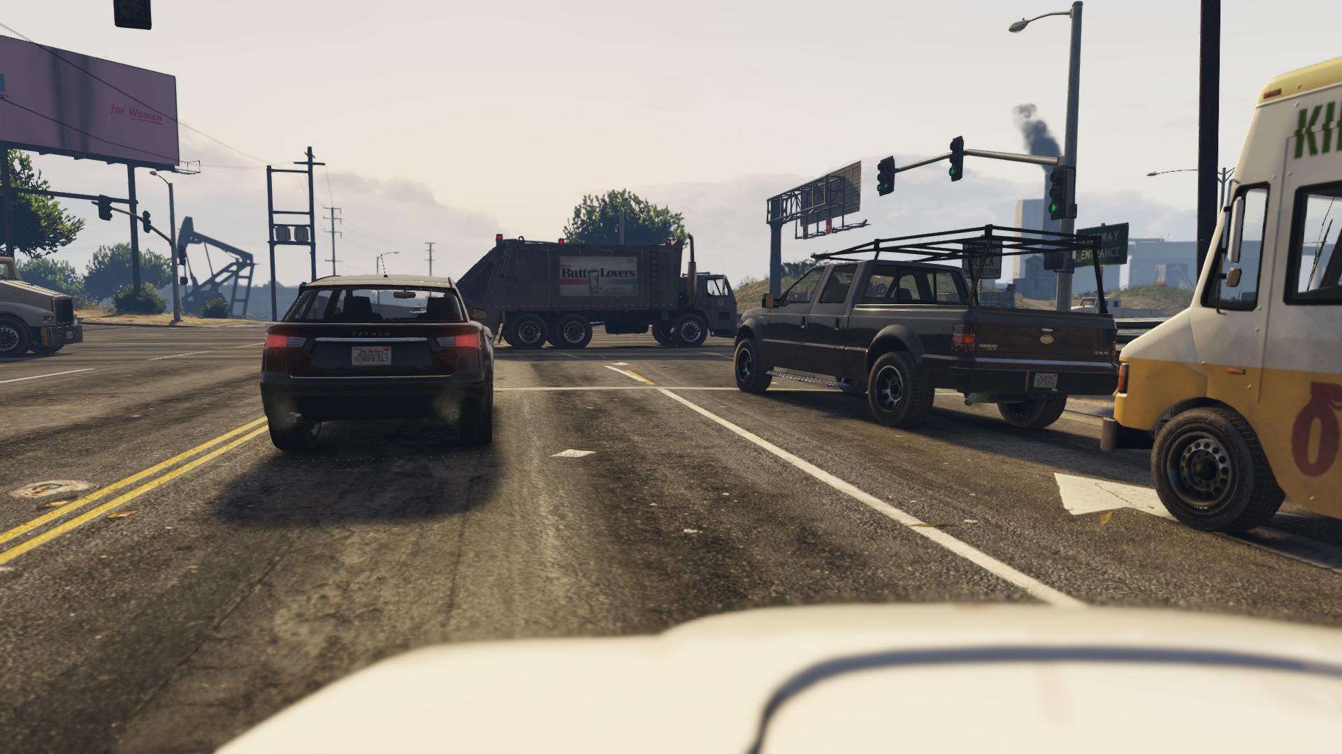
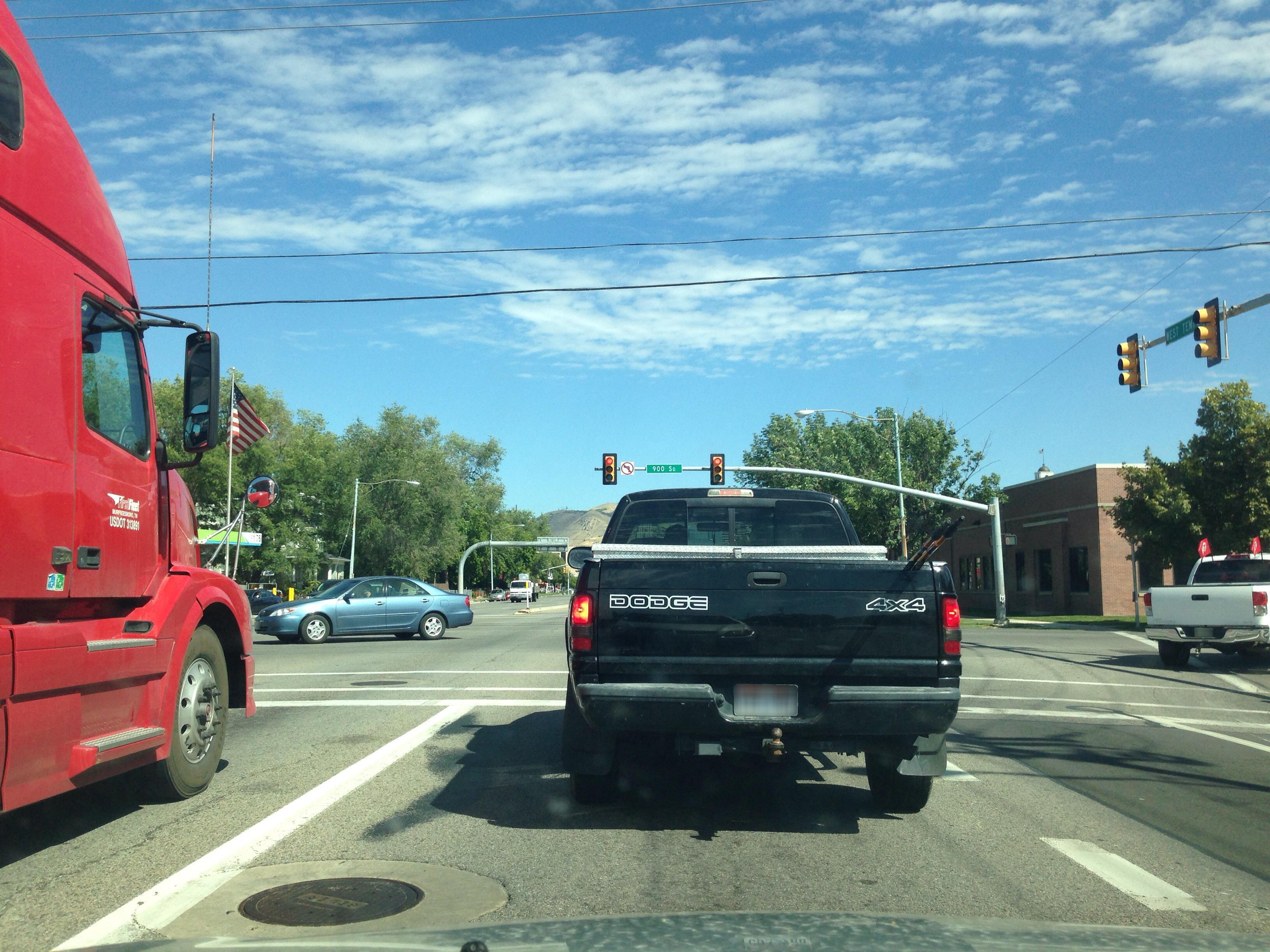
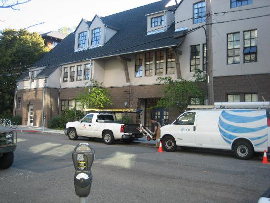
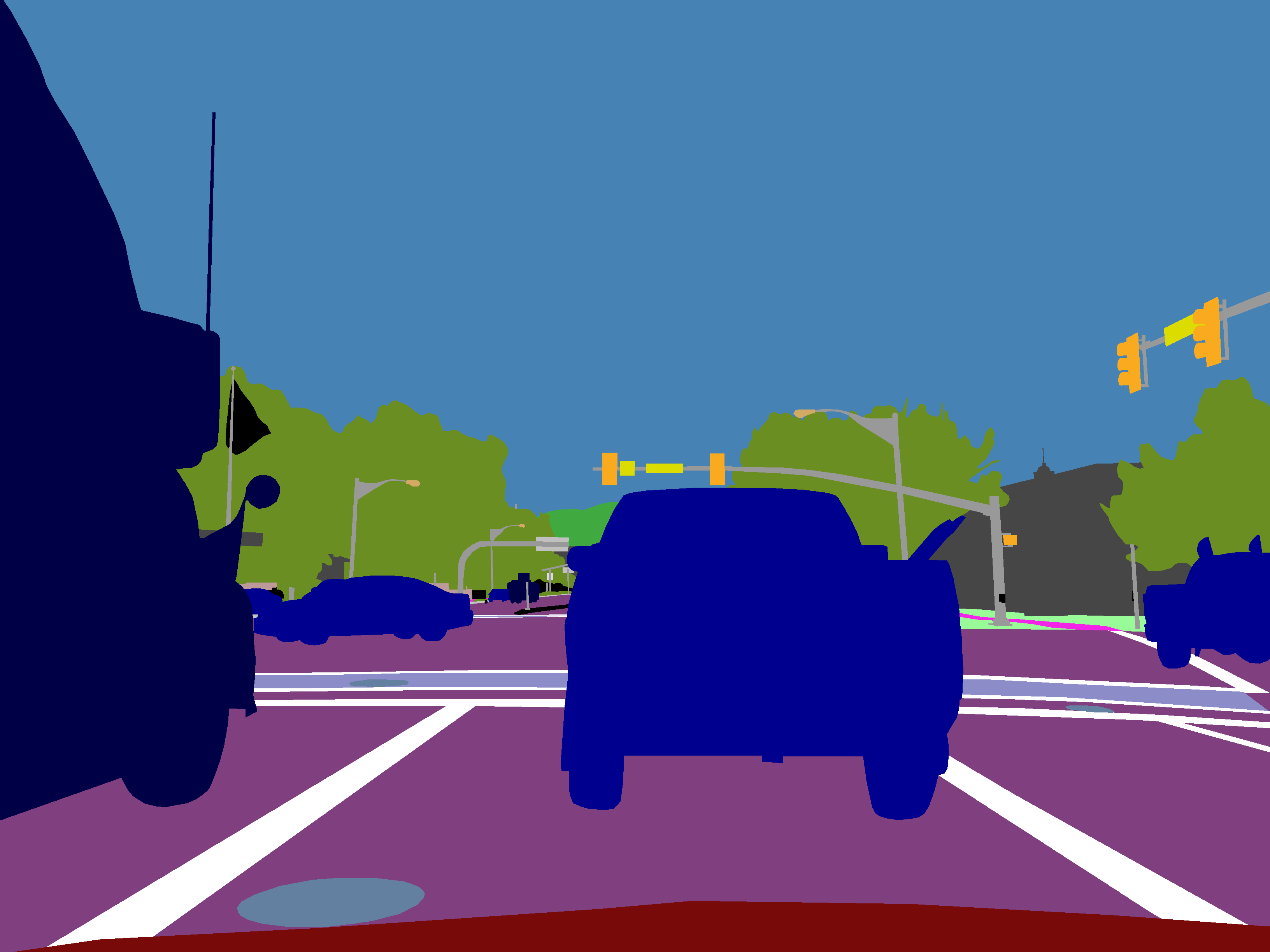
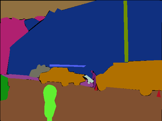
Training on multiple datasets is especially interesting for dense prediction models due to very expensive labels [43]. However, this is not easily carried out in practice since existing datasets use incompatible taxonomies [16, 15]. These incompatibilities may be caused by discrepant granularity and overlapping classes. Discrepant granularity [16] arises where some class from dataset A corresponds to several classes from dataset B. For instance the class road in Cityscapes is further divided into 8 classes in Vistas: road, bike_lane, crosswalk_plain, marking_zebra, marking_other, manhole, pothole, and service_lane. Overlapping classes occur when visual concepts get inconsistently grouped across datasets. For instance class truck in VIPER [26] includes trucks and pickups. Class car in Vistas [21] includes cars, pickups and vans. Class van in Ade20k [41] includes vans and pickups. We say that VIPER truck overlaps Vistas car (and Ade20k van) since the corresponding pixels have non-empty intersection and non-empty set difference in both directions. Fig. 1 shows that the three datasets assign pickups into three different classes.

Figure 1: We address dense-prediction models which can learn visual concepts from multiple datasets with overlapping classes. Example: pickups are labeled as class truck in VIPER [26] (left), class car in Vistas [21] (middle) and class van in Ade20k [41] (right). We resolve the class overlap (Viper-truck vs Vistas-car vs Ade20k-van) by learning on partial labels [6].

This paper addresses two important challenges in multi-domain semantic segmentation: i) training on datasets with inconsistent labels, and ii) designing an experimental setup capable of learning hundreds of dense logits on megapixel resolution. We contribute a novel method for training semantic segmentation on datasets with discrepant granularity and overlapping classes by leveraging partial labels [6] and class-wise log-sum-prob loss. Our method builds a universal taxonomy such that each dataset-specific class can be expressed as a union of one or more universal classes. Our universal models can be seamlessly trained and evaluated on each individual dataset since probabilities of dataset classes correspond to sums of probabilities of universal classes.

Our method outperforms two baselines which ignore overlapping classes, as well as a recent approach [15] based on partial relabeling towards a closed unified taxonomy. Computational advantages of our method become decisive in large-scale multi-domain experiments where we achieve state-of-the-art performance on the RVC 2020 benchmark collection and the WildDash 2 benchmark.

2 Related Work

We consider efficient training on a collection of semantic segmentation datasets with discrepant granularities and overlapping classes. This requires a capability to learn fine-grained classes on coarse-grained labels. Thus, we review semantic segmentation, efficient architectures, learning with partial labels, and multi-domain dense prediction.

2.1 Semantic Segmentation

Deep convolutional models have spurred substantial progress in the field of semantic segmentation [19, 3, 39, 4]. Recent work improves recovery of the spatial details lost due to downsampling [3] and incraeses the receptive field [39]. U-Net [27] recovers the fine details by blending deep semantics with spatial information from the early layers. Further work notices that the upsampling path requires much less capacity than the recognition backbone [18, 13]. Increased subsampling enlarges the receptive field, improves efficiency and reduces the training footprint [2, 13]. Further shrinking of the training footprint can be achieved through gradient checkpointing [28, 14]. Multi-scale processing relaxes the requirements on recognition capacity and leads to competitive results with efficient backbones [24, 38]. HRNet [33] preserves fine details by sustaining high-resolution representations along the entire convolutional pipeline. Its improved variant uses attention pooling to promote pixels of the majority class [35].

2.2 Efficient inference and training

Several recent semantic segmentation architectures aim at high accuracy while supporting real-time inference [2, 22, 24, 10, 38]. Most of these approaches can be trained at a fraction of the computational budget required by widely used methods. Hence, efficient architectures may create new opportunities while making our research more inclusive and environmentally acceptable [29].

2.3 Partial labels and log-sum-prob loss

Log-sum-prob loss allows to train unions of disjoint predictions by aggregating over classes or data. Data-wise formulation has been used to decrease influence of noisy labels [42]. Their loss sums probabilities of all labels from the $3\times 3$ neighborhood in pixels near semantic borders. On the other hand, our loss performs class-wise aggregation by summing probabilities of all universal classes corresponding to the coarse-grained label. Our motivation is to allow learning over inconsistent taxonomies, while they alleviate inaccurate annotations at semantic boundaries.

Learning from partial labels considers examples labeled with a set of classes only one of which is correct. The original work [6] assumes fairly stochastic probability $P(\mathbbmsl{Z}|\bm{x},y)$ of false labels $\mathbbmsl{Z}$ given the datum $\bm{x}$ and its true label $y$. In our context, this relation is deterministic when the dataset of the datum is known. Different from [6], we formulate learning with partial labels in a principled probabilistic framework based on log-sum-prob loss.

Recent work [40] considers partial labels for multi-domain object detection. Their experiments show that log-sum-prob loss does not contribute to object detection which is likely due to the sheer asymmetry between positive and negative windows. On the other hand, our experiments indicate that log-sum-prob loss and partial labels are an effective tool for cross-dataset semantic segmentation.

2.4 Multi-domain dense prediction

Multi-domain dense prediction involves training on multiple datasets with different taxonomies. A simple baseline consists of a shared encoder and separate per-dataset decoders [12]. This is similar to training on naive concatenation of individual datasets. We find this to be suboptimal since repetition of classes (eg. Vistas-bus vs Ade20k-bus) increases the memory demands and decreases utility of predictions. Instead, we prefer to train on a shared universal taxonomy which contains much less classes and supports inference on novel datasets.

A universal taxonomy can be implemented as a hierarchy of logits for categories and classes [16, 20]. This approach can gracefully handle datasets with discrepant granularities. However, on the downside, it requires very complex training and can not train on overlapping classes.

A universal taxonomy can also be implemented as a flat vector of universal logits [15, 40]. The only such semantic segmentation approach [15] does not train on heterogeneous datasets. Instead, they propose to adapt all datasets towards a unified taxonomy of their own. This requires relabeling all datasets which do not distinguish classes from their universal taxonomy, and merging all classes which are more fine-grained than the universal taxonomy. It would be impractical for such unified taxonomy to include all dataset classes, since that would imply unacceptable relabelling effort. Consequently, such design does not allow evaluation on original datasets nor simple introduction of datasets with novel taxonomies.

As mentioned in 2.3 a recent multi-domain object-detection approach [40] considers candidate windows which may correspond either to the background or to any of the non-annotated classes. Their attempt to solve that problem with log-sum-prob loss was not successful. However, classes of coarse-grained datasets usually group visual concepts which are much much more similar to each other than to a catch-all background class. Consequently, log-sum-prob training may have better a chance for success in multi-domain semantic segmentation.

Different than all previous approaches, we present a principled method for cross-dataset and multi-domain training of semantic segmentation models. We assemble a universal flat taxonomy from an almost unconstrained collection of datasets. The recovered universal taxonomy allows to seamlessly train and evaluate a universal probabilistic model on unchanged individual datasets by relying on partial labels and log-sum-prob loss. The resulting models are suitable for universal semantic segmentation in the wild.

3 Multi-domain semantic segmentation

We present a principled method for simultaneous training on semantic segmentation datasets with incompatible labeling policies. Our method builds a universal taxonomy which gathers and refines semantics of individual datasets by expressing each dataset class as a union of universal classes. Our models learn to predict universal classes while fully supporting training and evaluation according to individual datasets. We take care to contain the memory footprint of our models since effective multi-domain learning requires large crops and large batches.

3.1 Terminology and notation

We consider semantic classes $c$ as sets of pixels in all possible images and use set notation to express relations between them. For example: Vistas-sky = CS-sky, CS-road $\supset$ Vistas-manhole, VIPER-truck $\cap$ Vistas-car = WD-pickup, CS-road $\perp$ CS-car $\Rightarrow$ CS-road $\cap$ CS-car = $\emptyset$. Note that WD and CS stand for WildDash 2 and Cityscapes, respectively.

A set of mutually disjoint semantic classes defines a flat taxonomy $\mathbbmsl{S}_{d}=\{c_{t}\},c_{i}\perp c_{j},\forall i,j\colon i\neq j$. We note that a union of flat taxonomies is not guaranteed to be a true taxonomy since members may have non-empty intersections. For example, ${\mathbbmsl{S}}_{\text{VIPER}}\cup{\mathbbmsl{S}}_{\text{Vistas}}$ is not a true taxonomy since VIPER-truck $\not\perp$ Vistas-car (cf. Fig. 1).

A semantic segmentation dataset consists of images and corresponding dense labels: $\mathbbmsl{D}=\{(\bm{x}_{k},\bm{y}_{k})\}$. The labels assign semantic classes $c\in\mathbbmsl{S}_{d}$.

3.2 Baseline approach: naive concatenation

We consider training a semantic segmentation model on a compound dataset $\bigcup_{d}\mathbbmsl{D}_{d}$. This can not be accomplished by relying on individual taxonomies $\mathbbmsl{S}_{d}$, since that would either entail information loss (eg. remapping Vistas-manhole to CS-road), or require expensive relabeling (eg. remapping some pixels from CS-road to Vistas-manhole).

We propose a simple baseline approach which creates a training taxonomy as a naive concatenation of all individual taxonomies $\mathbbmsl{S}_{d}$. Each training taxonomy is mapped onto the corresponding subset of universal labels. For instance, cars from Cityscapes are mapped to the class Cityscapes-car, while cars from Vistas are mapped to Vistas-car. The predictions are produced by a single softmax over $\sum_{d}|\mathbbmsl{S}_{d}|$ logits, which allows training with the cross-entropy loss.

However, the described approach does not produce a true taxonomy, and thus leads to contention between overlapping logits (e.g. CS-road vs Vistas-road). This wastes model capacity due to need for dataset recognition instead of promoting generalization by principled dealing with ambiguous supervision. Additionally, the class replication increases the number of logits. This may hurt recognition of rare classes and exhaust GPU memory since the predictions are produced on a large resolution. Finally, inference has to deal with starvation of overlapping logits which we alleviate with post-inference mappings (cf. 3.5).

3.3 Baseline approach: partial merge

Naive concatenation can be improved by merging classes which match exactly; for example, Cityscapes-sky and Vistas-sky can be merged into the universal class sky. Classes which can not be matched in a 1:1 manner remain separate (e.g. Cityscapes-road, Vistas-road and Vistas-marking). This is similar to naive merge from [15], however we merge according to semantics instead of symbolic names and use post-inference mappings as described in 3.5. This may reduce the amount of capacity needed to distinguish between datasets due to eliminated contention between the merged classes. Nevertheless, partial merge also fails to produce a true taxonomy since overlapping classes remain unresolved. Hence, we encounter the same problems as presented in 3.2 although to a lesser extent.

3.4 Creating a universal taxonomy

We address disadvantages of the two baselines by building a flat universal taxonomy $\mathbbmsl{U}$ which will allow i) training on overlapping labels (cf. 3.6), and ii) seamless dataset-specific (cf. 3.5) or dataset-agnostic evaluation. The desired universal taxonomy $\mathbbmsl{U}$ should have the following properties. First, its classes should encompass the entire semantic range of individual datasets: $\bigcup_{u\in\mathbbmsl{U}}u=\bigcup_{d}\mathbbmsl{S}_{d}$. Second, universal classes should be disjoint: $\forall u,u^{\prime}\in\mathbbmsl{U}\colon u\perp u^{\prime}$. Third, no universal class may have a non-empty difference towards an intersecting dataset-specific class: $\forall u\in\mathbbmsl{U},c\in\bigcup_{d}\mathbbmsl{S}_{d}\colon(u\perp c)\vee(u\subseteq c)$. Such taxonomy will allow us to define mappings $m_{\mathbbmsl{S}_{d}}\colon\mathbbmsl{S}_{d}\to 2^{\mathbbmsl{U}}$ from dataset-specific classes to subsets of the universal set.

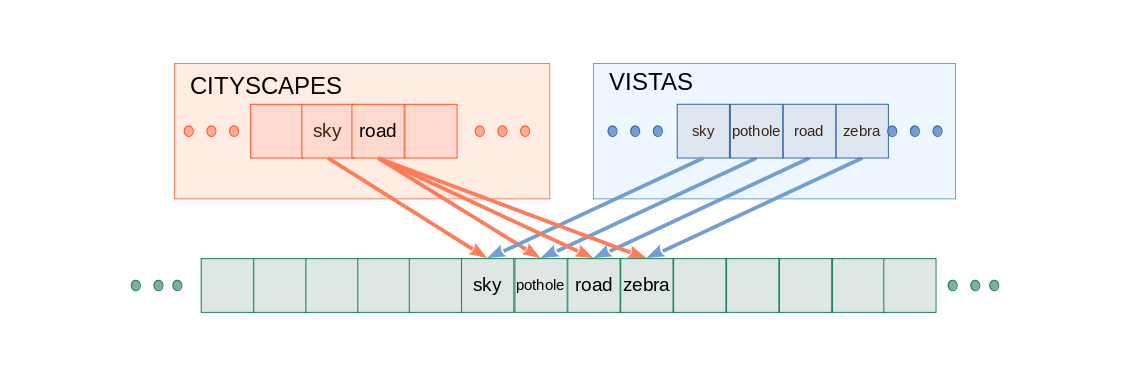
We propose to recover the universal taxonomy $\mathbbmsl{U}$ by iteratively transforming a multiset $\mathbbmsl{M}$ that contains dataset specific classes from all datasets. We apply the rules following rules until all of the classes are disjoint.

1. If two classes $c_{i}$ and $c_{j}$ match exactly, we merge them into a new class $c^{\prime}$ and map $c_{i}$ and $c_{j}$ to $c^{\prime}$.
   Example: Since WD-sky and CS-sky are equal, we merge them into a class sky, and define new mappings: WD-sky $\mapsto$ sky, CS-sky $\mapsto$ sky.

2. If a class $c_{i}$ is a superset of a class $c_{j}$, then $c_{i}$ is mapped to $\{c_{j},c_{i}^{\prime}\}$ where $c_{i}^{\prime}=c_{i}\setminus c_{j}$.
   Example: KITTI-car is a superset of car because it contains vans. We therefore add van as a new class and create a mapping KITTI-car $\mapsto$ {car, van}.

3. If two classes overlap, $(c_{i}\not\perp c_{j})$ $\wedge$ $(c_{i}\setminus c_{j}\neq\emptyset)$ $\wedge$ $(c_{j}\setminus c_{i}\neq\emptyset)$, $c_{i}$ and $c_{j}$ are replaced with three new disjoint classes $c_{i}^{\prime}=c_{i}\setminus c_{j}$, $c_{j}^{\prime}=c_{j}\setminus c_{i}$, and $c^{\prime}=c_{i}\cap c_{j}$. Class $c$ is mapped to $\{c_{i}^{\prime},c^{\prime}\}$, while $k$ is mapped to $\{c_{j}^{\prime},c^{\prime}\}$.
   Example: VIPER-truck contains trucks and pickups while Ade20k-truck contains trucks and trailers. We therefore replace VIPER-truck and Ade20k-truck with truck, pickup and trailer and create the following mappings: VIPER-truck $\mapsto$ {truck, pickup} and Ade20k-truck $\mapsto$ {truck, trailer}

3.5 Mapping predictions to target classes

In practice, universal models are evaluated on particular dataset-specific taxonomies. We therefore design evaluation mappings from dataset specific taxonomy $\mathbbmsl{S}_{d}$ to the training class set $\mathbbmsl{T}$. We extend $\mathbbmsl{S}_{d}$ with a void class. In our experiments, $\mathbbmsl{T}$ is either one of the two baselines or the universal taxonomy $\mathbbmsl{U}$, while $\mathbbmsl{S}_{d}$ corresponds to the particular dataset (e.g. $\mathbbmsl{S}_{d}=\mathbbmsl{S}_{\text{CamVid}}$). We can create evaluation mappings according to the following rules:

1. Each dataset-specific class is mapped to all training classes it overlaps with: $c^{S_{d}}\mapsto\{c^{T}\in\mathbbmsl{T}\colon c^{S_{d}}\not\perp c^{T}\}$.

2. The void class is mapped to all training classes which do not overlap with any of the dataset-specific classes: $\mathrm{void}\mapsto\{c^{T}\in\mathbbmsl{T}\colon\forall c^{S_{d}}\in\mathbbmsl{S}_{d},c^{S_{d}}\perp c^{T}\}$.

We can use the created mappings to calculate the classification score for each dataset-specific class in each pixel:

$$\mathrm{S}({Y}^{S_{d}}=c|\bm{x})=\sum_{t\in m_{\mathbbmsl{S}_{d}}(c)}\operatorname{P}({Y}{T}=t|\bm{x})\;.$$ (1)

In the case of the universal taxonomy, the above score corresponds to probability since each universal class occurs in the mapping set of exactly one dataset-specific class. In the case of the two baselines, the score has to be renormalized because training classes may overlap with several dataset-specific classes, e.g. $\mathrm{S}$(Vistas-pothole$|\bm{x}$) = $\mathrm{P}$(cs-road$|\bm{x}$) + $\mathrm{P}$(vistas-pothole$|\bm{x}$), $\mathrm{P}$(Vistas-pothole$|\bm{x}$) = $\mathrm{S}$(Vistas-pothole$|\bm{x}$) / $\sum\mathrm{S}(c^{S_{d}}_{j}|\bm{x})$. Thus, creation of post-inference mappings for the two baselines requires almost the same effort as the design of our universal taxonomy.

3.6 Learning a universal model with partial labels

We propose to learn cross-dataset models on the universal taxonomy $\mathbbmsl{U}$ in order to properly address overlapping labels while fully exploiting all available supervision. The resulting universal models will overcome all disadvantages of the two baselines. In particular, they will be capable to exploit partial supervision while being applicable in the wild.

Let us model the probability of universal classes as per-pixel softmax over $|\mathbbmsl{U}|$ logits $\bm{s}$. Let the random variable $Y$ denote a universal model prediction at that pixel, and let $\bm{p}$ denote the softmax output. Then we can write: $p_{u}=\operatorname{softmax}(\bm{s})_{u}=\operatorname{P}(Y=u|\bm{x})$. Hence, the negative log-likelihood of the probability of a dataset-specific class $c$ can be expressed as:

$$\mathcal{L}^{\text{NLL+}}(\bm{p},c)=-\ln\sum_{u\in m_{\mathbbmsl{S}_{d}}(\bm{c})}p_{u}\;.$$ (2)

Note that the sum of $p_{u}$ can be considered as probability since our universal classes are disjoint by design. We denote the resulting log-sum-prob form as NLL+: negative log-likelihood of aggregated probability. This loss becomes the standard negative log-likelihood when $|m_{\mathbbmsl{S}_{d}}(c)|=1$.

In order to better understand the NLL+ loss (2) we analyze its partial derivatives with respect to logits $\bm{s}$:

$$\frac{\partial\mathcal{L}}{\partial s_{u}}=p_{u}-{\mathinner{\mathopen{}\mathclose{{}\left\llbracket{u\in m_{\mathbbmsl{S}_{d}}(c)}}\right\rrbracket}}\frac{\exp{s_{u}}}{\sum_{k\in m_{\mathbbmsl{S}_{d}}(c)}\exp{s_{k}}}\;.$$ (3)

We observe that gradients w.r.t. incorrect logits are positive and the same as in the standard case, since then the second term is zero. Furthermore, the gradients w.r.t. labeled logits are always negative since the two terms have equal numerators, while the second term has a smaller denominator. If there are two correct logits, the larger one will have an exponentially larger numerator of the second term, while the denominator will be the same. Hence the difference between the correct logits is likely to increase after the update.

This analysis indicates that NLL+ favours peaky sub-distributions over correct logits: the model is compelled to pick only one among them. In the limit, when one of the labeled logits becomes much stronger than its peers, its gradients become equal to the standard supervised case, provided that the chosen logit is correct. This suggests that partial labels may help whenever there exists some learning signal that supports recognition of individual universal classes.

Our GPU implementation represents each dataset mapping $m_{\mathbbmsl{S}_{d}}$ as an $|\mathbbmsl{S}_{d}|\times|\mathbbmsl{U}|$ binary matrix with unit column sums. Probabilities of dataset-specific classes are computed by multiplying this matrix with universal probabilities.

3.7 Efficient multi-domain semantic segmentation

Multi-domain semantic segmentation is an extremely computationally intensive task since the complexity of training may be in the petaFLOP range. The training footprint of the model is an important factor since the model performance improves with large batches, large training crops and increased number of channels along the upsampling path. These considerations are a compelling reason to prefer training on universal classes instead of on less principled options such as the two baselines presented before.

This discussion suggests that efficient approaches may represent a sensible choice for such problems. We therefore base our experiments on pyramidal SwiftNet [24]. All our models use three image scales and produce dense logits at 8$\times$ subsampled resolution. These logits are bilinearly upsampled to the full resolution.

We train our models with a compound loss which corresponds to the product of the boundary-aware (BA) factor and the NLL+ loss (2). The BA modulation factor prioritizes poorly classified pixels and pixels at boundaries [24]:

$$\mathcal{L}^{\text{BA}}(\bm{p},c) =-\alpha\cdot e^{\gamma(1-\vphantom{p}\smash[t]{\hat{p}})}\ln\vphantom{p}\smash[t]{\hat{p}},\;\text{where}\;\vphantom{p}\smash[t]{\hat{p}}=\!\!\!\!\!\!\sum_{u\in m_{\mathbbmsl{S}_{d}}(c)}\!\!\!\!\!p_{u}\;.$$ (4)

We note that memory efficency becomes extremely important when training with several hundred logits and large crops. Even a humble inference becomes a challenge in 2$\times$ upsampled Vistas images (24MPx) used in multiscale inference since then the logit tensor requires almost 20GB RAM. We avoid caching multiple activations at full resolution by implementing the boundary aware NLL+ loss (4) as a layer with custom backprop. This ensures a minimal increase of the training footprint with respect to the standard NLL formulation.

4 Experiments

We present semantic segmentation experiments on models based on pyramidal SwiftNet [24]. Most experiments are based on ResNet-18 [9], except our RVC models which use DenseNet-161 [11]. All our models are pre-trained on ImageNet. We train by optimizing the BA loss (4) (either NLL or NLL+) with Adam. We attenuate the learning rate from $5\cdot 10^{-4}$ to $6\cdot 10^{-6}$ by cosine annealing.

We train our validation models by early stopping with respect to the average mIoU across all datasets. Most of our models may emit predictions which cannot be mapped to any of the evaluation classes. For instance, Vistas-ego-vehicle is not labeled on Cityscapes. We map such predictions to void and count them as false negatives during calculation of the mIoU score.

We train on random square crops which we augment through resizing from 0.5$\times$ to 2$\times$ and horizontal flipping. The default crop size is 768. Our mini-batches favor images with multiple class instances and rare classes [28]. We also reweight the images so that the sum of image weights is equal for all of the datasets. This encourages fair representation of datasets and classes during training.

4.1 Comparison with two baselines

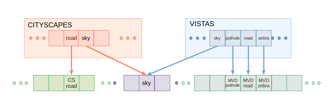
We compare our universal taxonomy with two baselines: naive concatenation (cf. 3.2) and partial merge (cf. 3.3). Both baselines require complex post-inference mapping before evaluation on particular datasets. For example joint training on Cityscapes and Vistas requires: {cs-sign, vistas-sign-front, vistas-sign-back, vistas-sign-frame} $\mapsto$ CS-sign. Some universal logits will be mapped to more than one evaluation class, eg: {cs-road, vistas-zebra} $\mapsto$ Vistas-zebra and {cs-road, vistas-pothole} $\mapsto$ Vistas-pothole. The merged training classes are 1:1 mapped to evaluation classes, eg; sky $\mapsto$ CS-sky and sky $\mapsto$ Vistas-sky.

We consider joint training on two pairs of road-driving datasets with incompatible taxonomies. We train for 100 epochs with batch size 18 which is the maximum that can fit into one Tesla V100 for the naive concatenation models. Our first experiment considers Cityscapes and Vistas. In this case, our universal taxonomy (cf. 3.4) corresponds to the Vistas taxonomy since it is a strict refinement of Cityscapes. Our universal taxonomy has 65 classes, which is less than the naive union (93) and the partial merge (72).

Our second experiment considers joint training on Vistas and WildDash 2 (WD2) [36]. We form WD2 minival by collecting the first 572 images and use all remaining images as WD2 minitrain. This setup is different from the first one since WD2 is much more diverse than Cityscapes. Hence, the baselines are going to have a harder time to recognize particular datasets according to the camera type or location. Additionally, WD2 has more classes than Cityscapes and a finer granularity of car types than Vistas. Consequently, our universal taxonomy has 67 classes which is less than the naive concatenation (98), and the partial merge (76).

Table 1 shows that the proposed universal taxonomy succeeds to outperform both baselines in spite of reduced capacity due to less logits. The advantage is especially evident in the case of joint training on WD2 and Vistas. We hypothesize that this occurs due to reduction of contention between overlapping classes, which allows the model capacity to be more efficiently exploited. Our universal taxonomy also outperforms the baselines on City-Vistas although the advantage is smaller than on WD2-Vistas. We explain this as follows. First, all Cityscapes images have been acquired across a contained geographical region with the same camera model. This makes dataset detection an easy task and hence alleviates class contention within the baselines. Second, this setup entails a smaller difference between our taxonomy and the partial merge (City-Vistas: 7 logits vs WD2-Vistas: 9 logits). We notice that our universal taxonomy outperforms individual training (Cityscapes: 0.5pp, Vistas: 0.1pp [24]), as well as that training on WD2-Vistas slightly reduces Vistas performance. This indicates that WildDash 2 requires more capacity than Cityscapes.

Taxonomy		(City-Vistas)			(WD2-Vistas)
		City	Vistas		WD2	Vistas
naive concat		76.8	44.6		55.3	43.1
partial merge		77.1	44.5		54.7	44.1
universal (ours)		77.0	44.9		56.2	44.4

Table 1: Evaluation of joint training on Cityscapes and Vistas (City-Vistas), as well as on WildDash 2 and Vistas (WD2-Vistas). Our universal taxonomy outperforms both baselines.

4.2 Cross-dataset evaluation

We explore models from Table 1 on novel road-driving datasets: CamVid test [1], KITTI train [8], BDD val [34] and IDD val [32]. We also evaluate the City-Vistas model on WildDash V2 minival and the Vistas-WD2 model on Cityscapes val. As before, we design mappings from each of the six training taxonomies to each evaluation taxonomy, and consider all unmapped logits as class void.

Tables 2 and 3 show that our taxonomy outperforms naive concatenation and partial merge on most foreign datasets, while in the remaining few cases the difference is within variance. Note that KITTI has only 200 images and is very similar to Cityscapes. As before, our contribution is greater on WD2-Vistas than City-Vistas. We connect that with Cityscapes peculiarities which discourage generalization, as discussed in 4.1.

Model	WD2	CV	KITTI	BDD	IDD
naive concat	43.3	74.1	58.9	56.7	42.4
partial merge	43.8	73.9	59.4	57.0	43.0
universal (ours)	43.9	75.3	60.5	58.0	42.8

Table 2: Cross-dataset evaluation of joint training on Cityscapes and Vistas. We evaluate the three models from Table 1 on WildDash 2 mini val, CamVid test, KITTI, BDD val, and IDD val.

Model	CS	CV	KITTI	BDD	IDD
naive concat	69.0	72.7	53.6	56.1	41.6
partial merge	69.8	72.4	53.5	57.1	41.9
universal (ours)	71.4	74.9	53.0	59.0	42.6

Table 3: Cross-dataset evaluation of joint training on Vistas and WildDash 2. We evaluate the three models from Table 1 on Cityscapes val, CamVid test, KITTI, BDD val, and IDD val.

4.3 Comparison with partial manual relabeling

Evaluation protocol	Taxono	Ade20k	BDD	Cityscapes	COCO	IDD	SUN RGBD	Vistas
Original	Universal (ours)	31.0	58.5	72.6	35.4	54.4	41.7	39.1
	MSeg	23.3	59.4	72.6	30.3	42.6	40.2	26.1
MSeg	Universal (ours)	34.5	58.5	72.6	36.3	53.0	41.7	45.4
	MSeg	34.3	59.4	72.6	34.9	55.6	40.2	43.6

Table 4: Multi-domain experiments with SNp-RN18 on the seven MSeg datasets [15]. We train a NLL+ model on original labels, and compare it with a NLL model which trains on manually relabeled images according to the MSeg taxonomy [15]. Both models are evaluated on validation subsets of Ade20k, BDD, Cityscapes, Coco, IDD, SUN RGB-D and Vistas. We consider all unmapped logits as class void.

We consider 7 datasets from different domains: Ade20k [41], BDD [34], Cityscapes [5], Coco [17], IDD [32], SUN RGBD [30] and Vistas [21]. Previous work has partially relabeled these datasets in order to make them fully compatible with a custom unified taxonomy called MSeg [15]. However, they had to omit 100 classes in order to contain the relabeling effort. We explore this trade-off by comparing identical models trained with: i) our universal taxonomy, original datasets and 294-way NLL+ loss, and ii) MSeg taxonomy, relabeled datasets, and 194-way NLL loss.

We resize each training image so that its smaller side is 1080 pixels, sample random square crops between 256$\times$256 and 1024$\times$1024, and resize them to 512$\times$512. We train both models on a single Tesla V100 for 20 epochs with batch size 20. We validate the two models according to the following two protocols. The MSeg protocol only evaluates the 194 classes from the MSeg taxonomy [15], while the original protocols evaluate all classes.

The top section of Table 7 presents evaluation according to the original protocol. Our approach prevails on most datasets due to capability to predict all 294 classes. The bottom section of the table shows that training with NLL+ remains competitive even when we evaluate only on the 194 classes covered by the MSeg taxonomy. This suggests that our universal taxonomy represents a flexible alternative to custom taxonomies, especially in view of adding new datasets to the training collection (cf. 4.5).

4.4 Recognition of unlabeled concepts

This experiment explores whether our method is able to recognize unlabeled concepts. We partition Cityscapes train into two splits with approximately equal number of images and similar overall distribution of classes. The first split gathers images from Aachen to Hanover. It relabels all trucks, buses and cars into the class called ’four-wheels-vehicle’. The second split gathers images from Jena to Zurich and relabels bicycles, motorcycles and cars into the class ’personal-vehicle’. Both splits have 17 classes. Buses, trucks, motorcycles and bicycles are labeled as standalone classes in only one of the two splits (roughly, half of the images), while cars are never labeled as a standalone class. Our universal taxonomy corresponds to 19 Cityscapes classes. The dataset class four-wheel-vehicle maps to {car, bus, truck}. The dataset class personal-vehicle maps to {car, bicycle, motorcycle}. All other dataset classes map to themselves.

We validate four models for 19-way dense prediction. The baseline model ignores all pixels of aggregate classes and uses the standard NLL loss. Two models train on aggregate classes through our NLL+ loss (4) and its variant which replaces the sum with max. The oracle uses the original Cityscapes train. We train all four models for 250 epochs with batch size 14 on GTX1080 while oversampling trains.

Table 5 reveals that NLL+ performs much closer to the oracle than to the NLL baseline. There is a substantial advantage for classes with only half non-ambiguous labels (bus, truck, motorcycle, bicycle), and especially on cars which are recognized as a novel concept at the intersection of two training labels. NLL-max [40] performs only slightly better than the NLL baseline, while NLL+ appears as a method of choice in presence of class overlap. The two baselines succeed to detect cars due to post-inference mapping, however NLL+ outperforms them substantially.

Model						mIoU
NLL baseline	0	54.2	43.9	32.5	60.3	58.7
NLL-max	0	9.6	40.8	1.6	75.7	61.8
naive concat	91.1	61.4	42.2	39.0	72.3	67.6
partial merge	92.4	54.3	55.1	39.0	74.3	71.4
NLL+	93.6	73.3	66.6	46.4	75.4	74.3
oracle	94.4	82.9	72.9	62.2	76.5	76.2

Table 5: Training on relabeled Cityscapes: one split aggregates cars, buses and trucks, while the other aggregates cars, bicycles and motorcycles. We validate NLL+ training, its NLL-max variant, and the NLL baseline which ignores all aggregate labels.

4.5 Large-scale multi-domain challenge

We present a large-scale multi-domain experiment on a benchmark collection proposed at the Robust Vision Challenge RVC 2020. The challenge requires submitting a single semantic segmentation model with less than 300 logits to seven benchmarks: Ade20k, Cityscapes, KITTI, Vistas, Scannet [7], Viper, and WildDash 2.

Figure 2: Qualitative performance of our SNp-DN161 submission to RVC 2020. Rows 1 and 3 show input images while rows 2 and 4 show the model predictions. Images belong to (top to bottom, left to right) ADE20k, Viper, KITTI, Cityscapes, WildDash, ScanNet and Vistas.

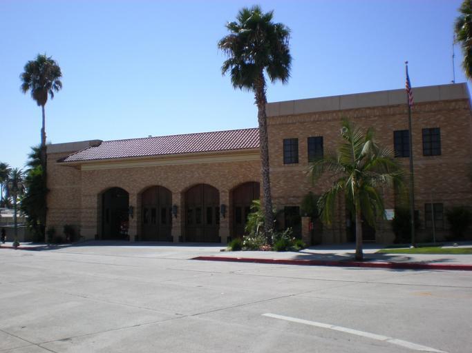
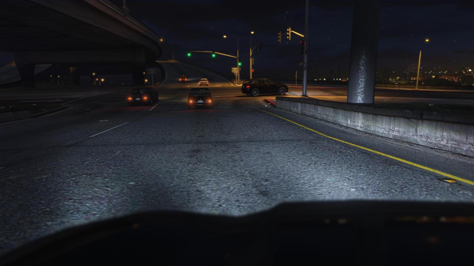
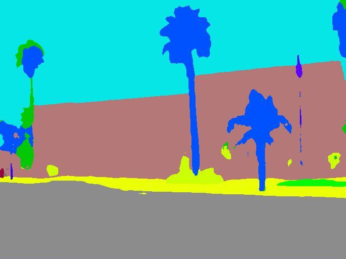
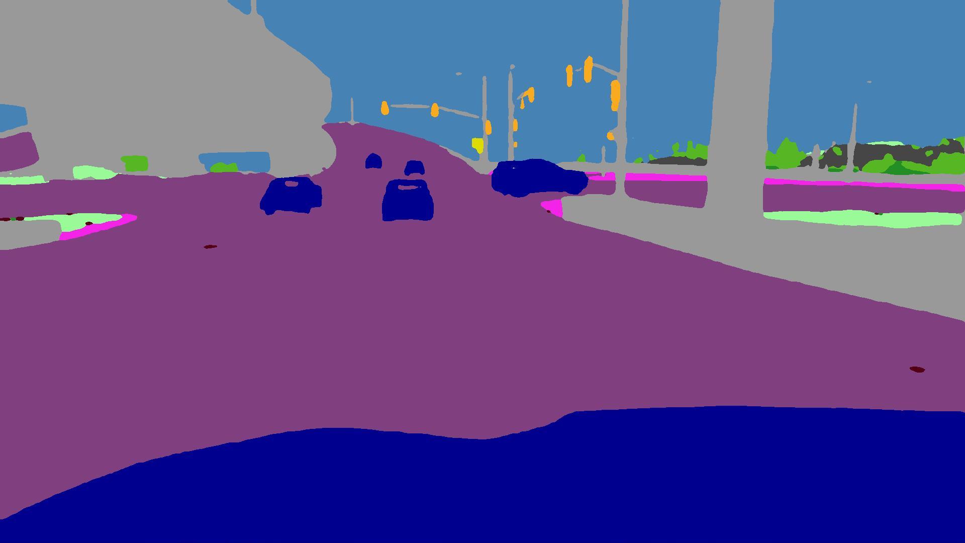
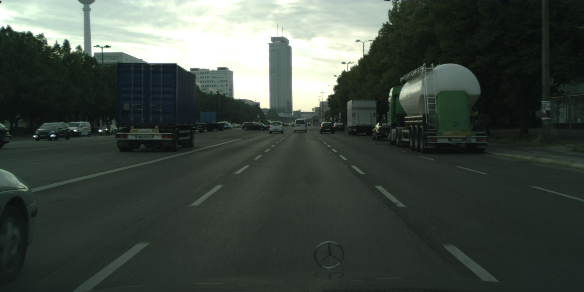
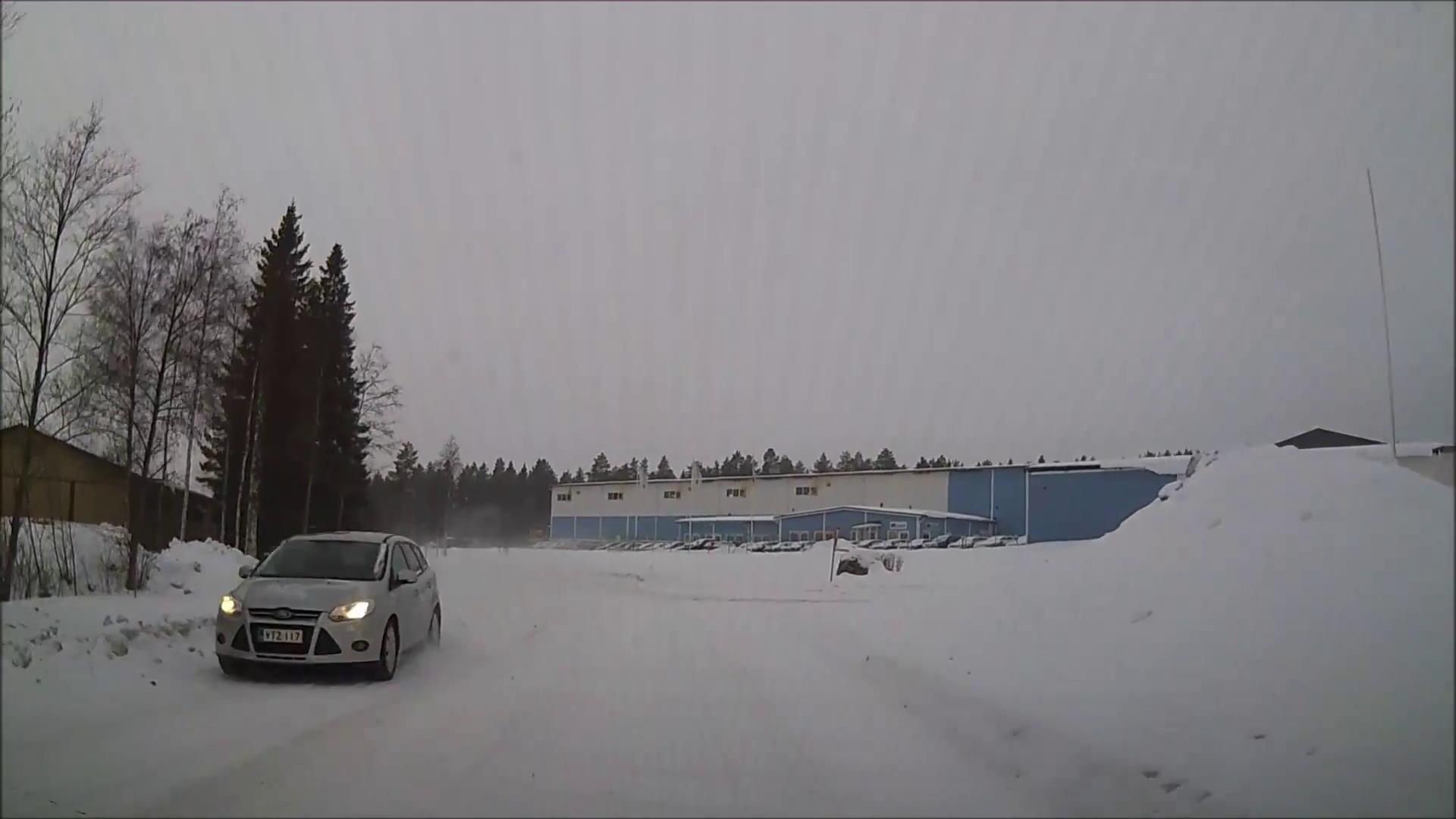
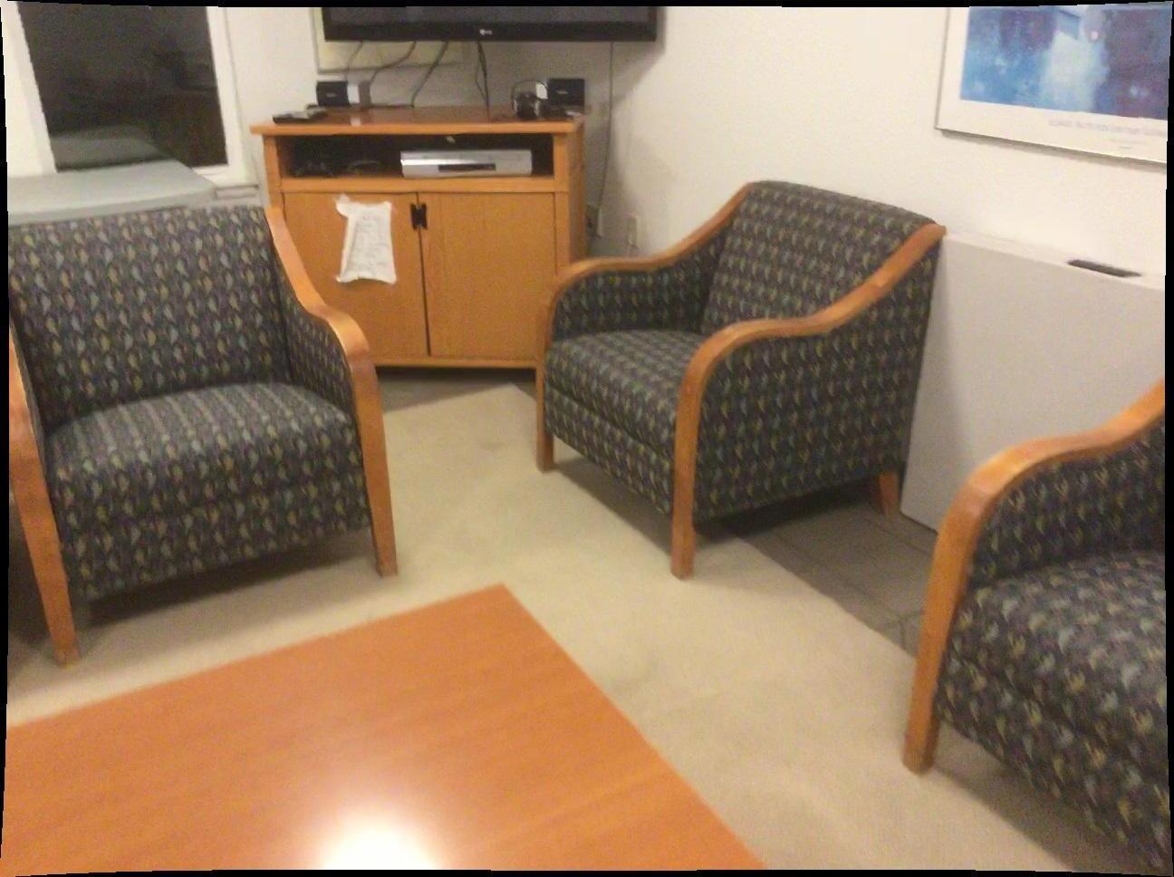
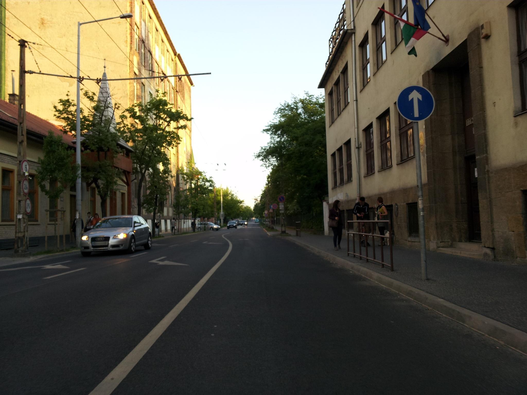
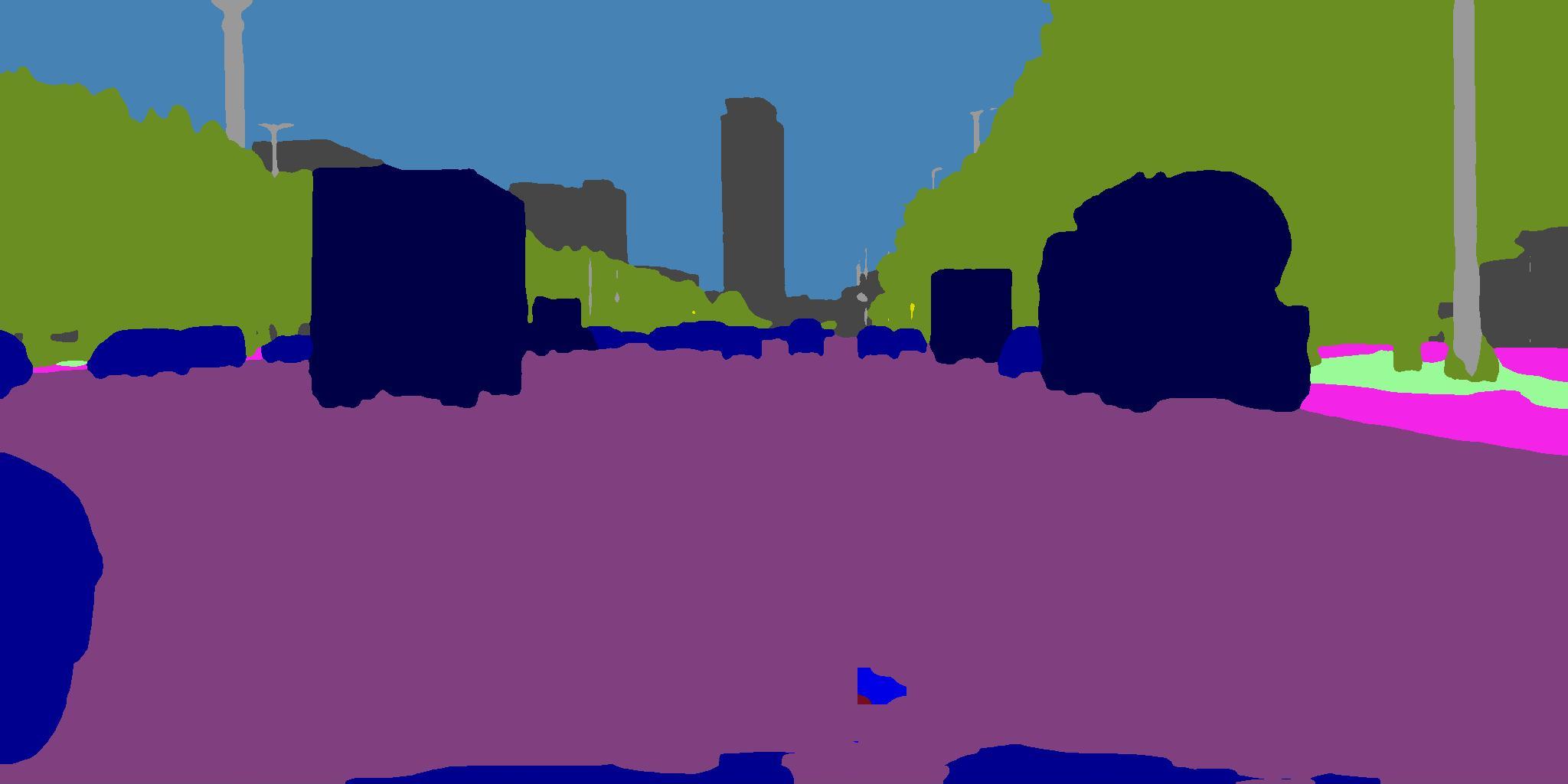
We recover a taxonomy of 192 universal classes according to the procedure from 3.4. It turns out that Vistas labels vehicle windows as vehicles, while VIPER labels these pixels with what is seen behind. A consistent resolution of this issue would effectively double the number of logits since most universal classes would require addition of their twin class (eg. person vs person_through_glass). Consequently, we introduce simplifying assumptions such as VIPER-car = Vistas-car and Vistas-car $\perp$ VIPER-person in order to reduce the training footprint of the universal model.

We increase the model capacity by using the DenseNet-161 [11] backbone and setting the upsampling width to 384 channels. We decrease the memory footprint with custom backprop and gradient checkpointing [28] in order to enable training on batches of 8 768$\times$768 crops per GPU.

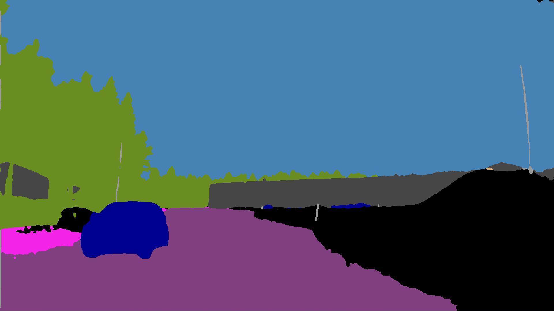
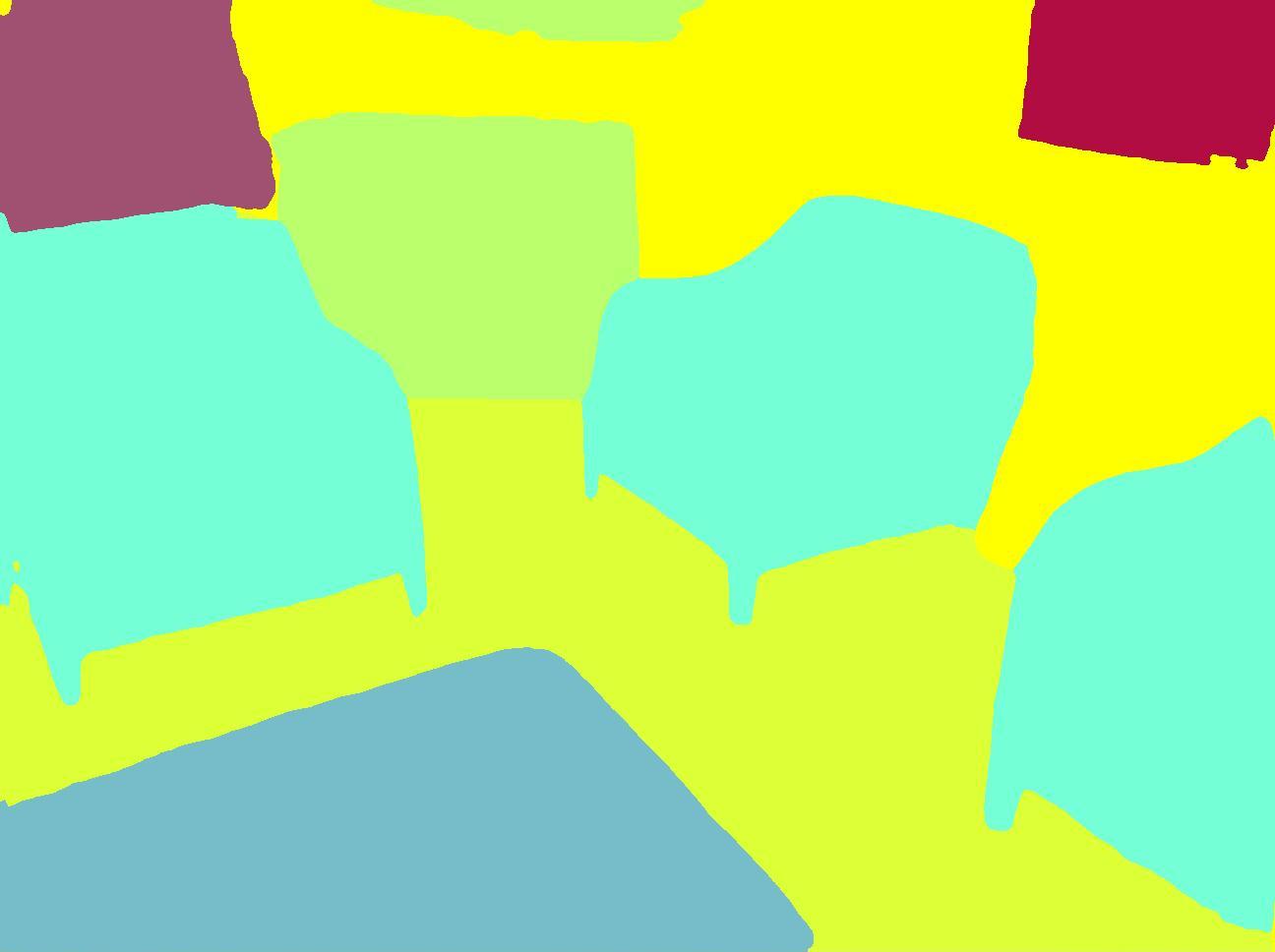
We train on seven datasets of the RVC 2020 collection on 6 Tesla V100 32GB for 100 epochs. We set the boundary modulation to 1 (minimum) for all ScanNet crops in order to alleviate noisy labels. We evaluate on six scales and two horizontal flips. Table 6 compares our model SNp_DN161 with the two valid submissions to RVC 2020 [23]. Fig. 3 presents qualitative performance of our model.

Model	ADE	CS	KIT	MV	SN	VIP	WD
MSeg1080	33.2	80.7	62.6	34.2	48.5	40.7	35.2
SN_rn152pyrx8	31.1	74.7	63.9	40.4	54.6	62.5	45.4
SNp-DN161	30.8	77.9	68.9	44.6	53.9	64.6	46.8

Table 6: Performance evaluation on RVC 2020 benchmarks Ade20k (ADE), Cityscapes (CS), KITTI (KIT), Vistas (MV), ScanNet (SN), VIPER (VIP) and WildDash 2 (WD). We compare the two valid RVC submissions (top) with our model (bottom).

We note that our model significantly outperforms the baseline submission MSeg1080_RVC [15] which is unable to predict any classes outside their closed unified taxonomy. This suggests advantage of open universal taxonomies such as ours, similarly as in 4.2. We believe that multi-domain training is instrumental for achieving robust performance in the real world. This is confirmed by the state-of-the-art performance of our RVC model on the WildDash 2 benchmark which is currently the only dataset which specifically targets expected points of failure of dense prediction models.

5 Conclusion

We have presented a principled method for cross-dataset training of semantic segmentation models. Our method allows seamless training and evaluation on multi-domain datasets with discrepant granularity and overlapping classes. Unlike simpler approaches such as multi-head prediction with shared features and dataset detection, our method recovers a universal taxonomy which transcends semantics of individual datasets. This allows transparent inference on novel datasets and promises thriving performance in the wild.

Our method expresses each dataset class as a union of disjoint universal classes. Hence, probabilities of dataset classes correspond to sums of probabilities of universal classes. This allows us to train a universal model on dataset-specific labels through negative log-likelihood of aggregated probability which we refer to as NLL+. Such training can be viewed as learning from partial labels since we train fine-grained universal classes on coarse-grained labels.

We compare our universal models to two baselines which ignore the overlap between dataset-specific logits. Our universal models outperform these two baselines in within-dataset generalization and cross-dataset validation. Experiments on relabeled Cityscapes indicate that our method is able to transcend semantics of individual datasets by learning an unlabeled universal concept at the intersection of overlapping dataset classes.

Validation on the MSeg collection shows that our method is competitive to standard NLL training on manually relabeled data. Our advantage becomes substantial when evaluating on original datasets where unified taxonomies have to drop classes in order to alleviate the relabeling effort.

Our method achieves the best aggregate performance on the 7 benchmarks from the RVC 2020 challenge. The corresponding universal taxonomy has only 192 classes, which is a considerable improvement over 311 classes in the naive concatenation. We see such multi-domain training as a method of choice for machine vision in uncontrolled environments. Indeed, our RVC models set a new state of the art on WildDash 2 — the toughest road-driving benchmark, while outperforming other approaches by a large margin.

The recovered universal models can be used as a tool for evaluating automatically recovered taxonomies. The authors would like to encourage further work on advanced evaluation datasets that will reward cross-dataset training and promote development of smarter and more robust visual systems. An ideal future dataset should combine rich taxonomies with domain shift, anomalous objects, out-of-domain context, and adversarial input. Other suitable avenues for future work include automatic recovery of universal taxonomies, extending the developed framework towards outlier detection and open-set recognition, and exploring knowledge-transfer potential of multi-domain universal models.

This supplement presents additional validation experiments and offers further qualitative analysis of our submission to RVC 2020. Additionally, it provides visualizations of our training and evaluation mappings for the two baselines and our universal taxonomy.

We use Adam and attenuate the learning rate from $5\cdot 10^{-4}$ to $6\cdot 10^{-6}$ by cosine annealing. We use the largest batch size that fits into the GPU memory, and train our models for 100 epochs. All these experiments use single-scale evaluation.

Appendix A Evaluation of the two baselines in multi-domain experiments

Evaluation protocol	Taxonomy	Ade20k	BDD	Cityscapes	COCO	IDD	SUN RGBD	Vistas
Original	naive concatenation	29.3	55.5	68.7	30.8	52.1	41.1	35.3
	partial merge	30	58.4	70.6	32.2	54.4	41.7	37.6
	MSeg	23.2	58.1	71.4	29	42.2	41.9	25.7
	Universal (ours)	31.3	56.5	71.2	33.7	53.1	42.5	37.9
MSeg	naive concatenation	32.3	55.5	68.7	31.5	53.9	41.1	41.4
	partial merge	33.3	58.4	70.6	32.9	51.8	41.7	43.9
	MSeg	34.3	58.1	71.4	33.5	53.9	41.9	43.0
	Universal (ours)	34.7	56.5	71.2	34.6	51.9	42.5	43.8

Table 7: Multi-domain experiments with SNp-RN18 on the seven MSeg datasets [15]. We train the baselines and our universal model on original labels, and compare with a NLL model trained on manually relabeled images according to the MSeg taxonomy [15]. Both models are evaluated on validation subsets of Ade20k, BDD, Cityscapes, Coco, IDD, SUN RGB-D and Vistas. We consider all unmapped logits as class void.

The main paper evaluates our universal taxonomy with a custom unified taxonomy called MSeg [15] in a multi-domain setup. We repeat that experiment with our two baselines, naive concatenation and partial merge, which in this setup have 469 and 307 classes. In order to have a consistent training setup, we train all four models on a single Tesla V100 32GB GPU. We use batch size 12, since that is the maximum for naive concatenation. We keep the rest of the training protocol the same as in the main paper.

The top section of Table 7 presents evaluation according to the original protocol. Our universal model prevails on most datasets. Partial merge performs comparably, since only 13 out of 307 classes overlap with some other class (our universal taxonomy has 294 classes). The bottom section of the table shows a similar outcome when we evaluate only on the 194 MSeg classes. We note that even naive union outperforms manual relabeling when original evaluation protocols are used since manual relabeling drops too many classes.

Appendix B Validation experiments

We validate several hyper-parameters on the Vistas dataset. In all tables the columns correspond to training resolution (MPx), total batch size (BS), number of computational nodes used for training (nPU), and segmentation accuracy on Vistas val (mIoU).

B.1 Validation of segmentation architectures

Table 8 shows performance of various semantic segmentation architectures on the validation subset of Vistas. We present best approaches from the literature and compare them with pyramidal SwiftNets with different backbones. All our models use checkpointed backbones and were trained on 1 Tesla V100 32GB GPU.

Model	MPx	BS	nPU	mIoU
Seamless [25]	8	8	8	50.4
HN-OCR-W48 [35]	0.5	16	2	50.8
PDL-X71 [4]	1	64	32	55.4
SNpyr-RN18	0.6	24	1	46.3
SNpyr-RN34	0.6	22	1	49.4
SNpyr-RN152	0.6	8	1	50.1
SNpyr-DN121	0.6	22	1	49.5
SNpyr-DN161	0.6	17	1	52.2

Table 8: Validation of semantic segmentation architectures. All methods use single-scale evaluation, and train on Tesla V100 32GB GPUs except PDL which trains on TPUs. Pyramidal Swiftnets achieve competitive performance with respect to the state of the art, while requiring much less computational resources.

The table shows that pyramidal SwiftNets offer competitive generalization performance under modest computational requirements. This makes them a good choice for large-scale experiments such as RVC 2020. Furthermore, larger models require significantly more time to complete the training, which may make a difference in large-scale multi-domain settings.

We observe that increasing the model capacity results in diminishing returns (cf. SNPyr-RN18 vs SNPyr-RN34 vs SNPyr-RN152). SNpyr-DN161 outperforms SNPyr-RN152 in spite a slightly weaker backbone. We speculate that this may be due to larger batches.

B.2 Validation of multi-scale input

Table 9 compares a pyramidal model (SNPyr-DN161s3) to its single-scale counterpart (SN-DN161s3). Both models are based on DenseNet-161 with 64$\times$ subsampled representation at the far end which we achieve by splitting the 3rd dense block [14]. The single scale model (SN-DN161s3) uses an SPP module at the end of the downsampling path at 64$\times$ subsampled resolution.

Model	MPx	BS	nPU	mIoU
SNpyr-DN161s3	0.6	18	1	50.6
SN-DN161s3	0.6	25	1	48.1

Table 9: Validation of pyramidal fusion. The multi-resolution model (SNpyr-DN161s3) outperforms its single-scale counterpart (SN-DN161s3).

B.3 Validation of upsampling width

Table 10 shows the influence of the upsampling width on the segmentation performance. Wider upsampling improves the accuracy, although not significantly.

Model	MPx	BS	nPU	mIoU
SNpyr-DN161s3	0.6	18	1	50.6
SNPyr-DN161s3-fat	0.6	18	1	50.9

Table 10: Validation of the width of the upsampling path. Wider upsampling path achieves a slightly better accuracy.

B.4 Validation of block splitting

Table 11 examines the influence of dense-block splitting to the generalization performance. We observe that splitting the 3rd block deteriorates the segmentation performance when pyramidal organization is used. We speculate that this is due to too much subsampling within the feature extractor.

Model	MPx	BS	nPU	mIoU
SNpyr-DN161	0.6	17	1	52.2
SNpyr-DN161s3	0.6	18	1	50.6

Table 11: Validation of the extent of subsampling within a multi-scale feature extractor. Splitting the third block reduces segmentation accuracy.

Appendix C Qualitative universal performance

Figure 3 extends Figure 2 from the main paper by including qualitative universal performance of our SNp-DN161 model. The color map for the universal label space combines the color maps from Vistas and ADE20k. We observe that the model is able to recognize refinements of concepts from particular datasets. For instance the model locates road markings and sidewalk curbs in images from Cityscapes, VIPER, KITTI and ADE20k. It also succeeds to discriminate bushes and trees in KITTI and WildDash 2 although this distinction exists only in the ADE20k taxonomy.

Figure 3: Qualitative performance of our universal SNp-DN161 model on test images from the seven RVC datasets. Rows 1 and 4 show input images, rows 2 and 5 show predictions in the universal label space, while rows 3 and 6 show dataset-specific predictions. Images belong to (top to bottom, left to right) ADE20k, Viper, KITTI, Cityscapes, WildDash, ScanNet and Vistas. Universal predictions find classes which are not labeled in the corresponding dataset, eg. crosswalk, curb and road-marking in the image from KITTI. All road driving datasets represent vegetation with a single class, but the universal model is able to classify those pixels more precisely as trees, palms and plants.

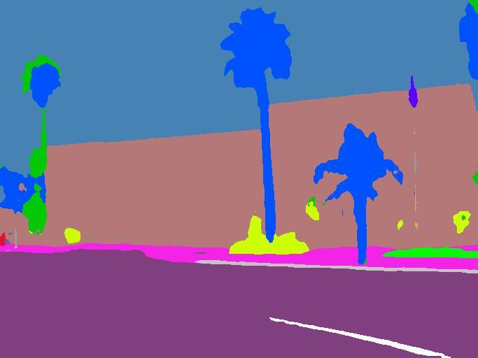
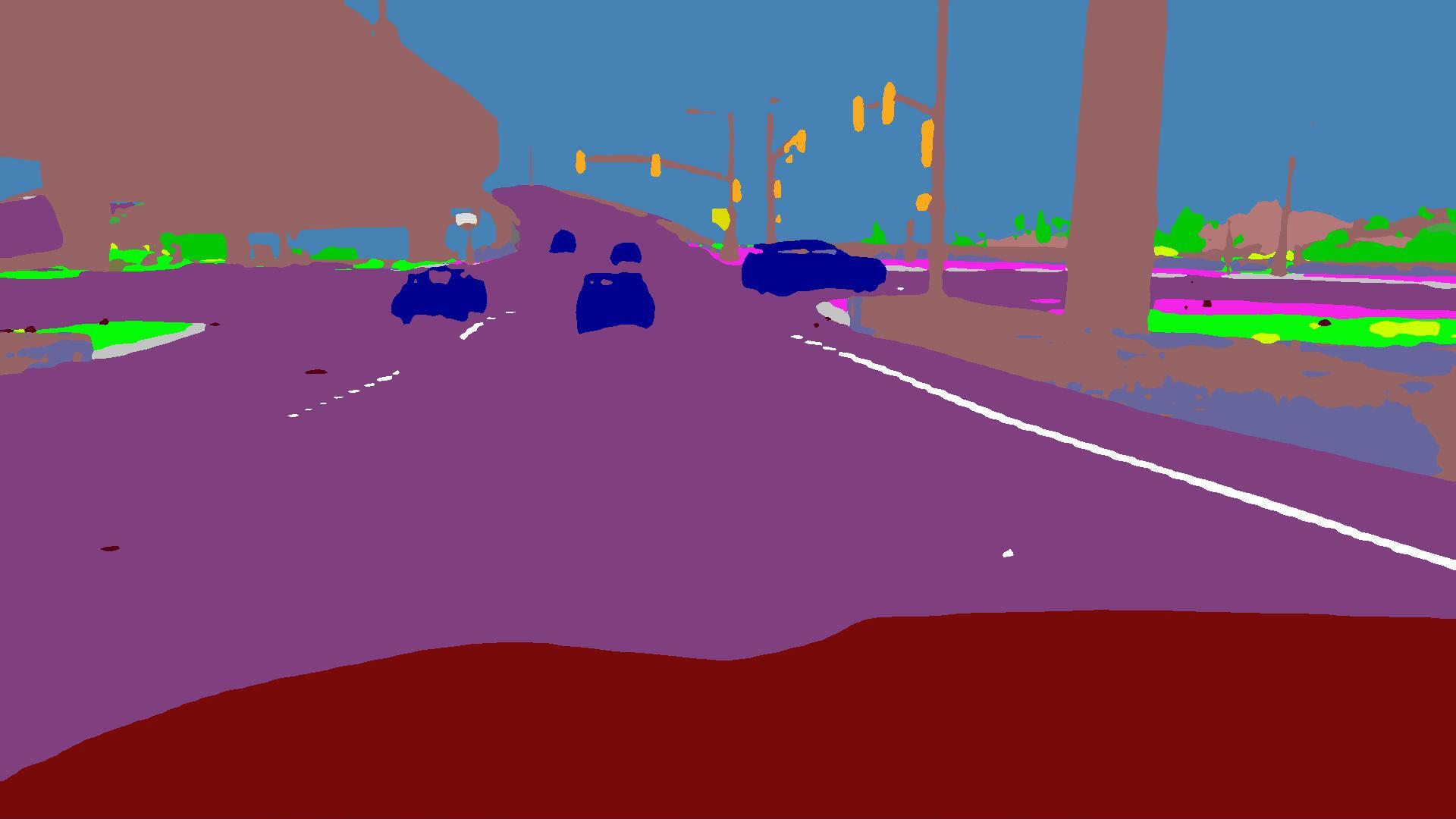
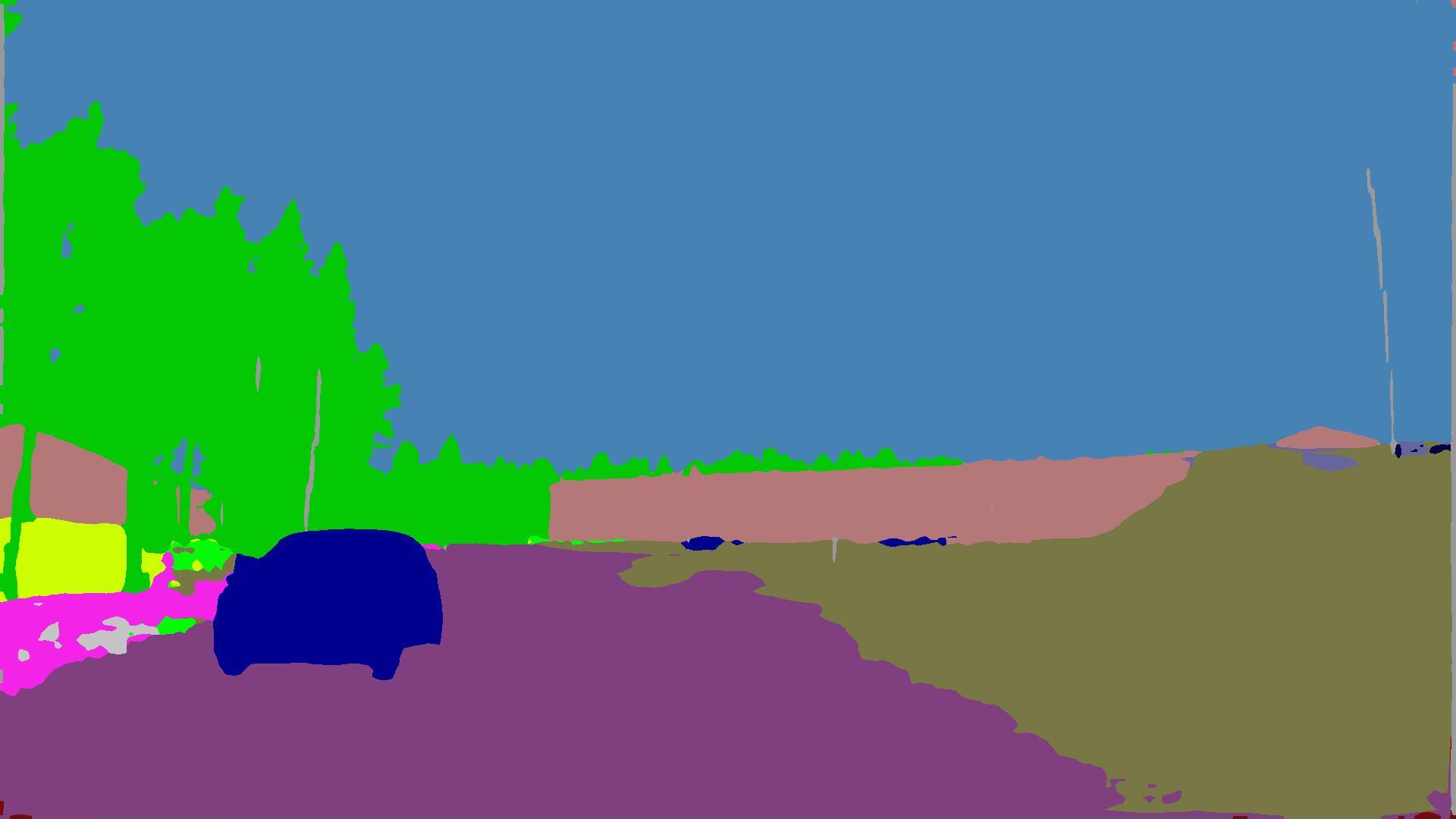
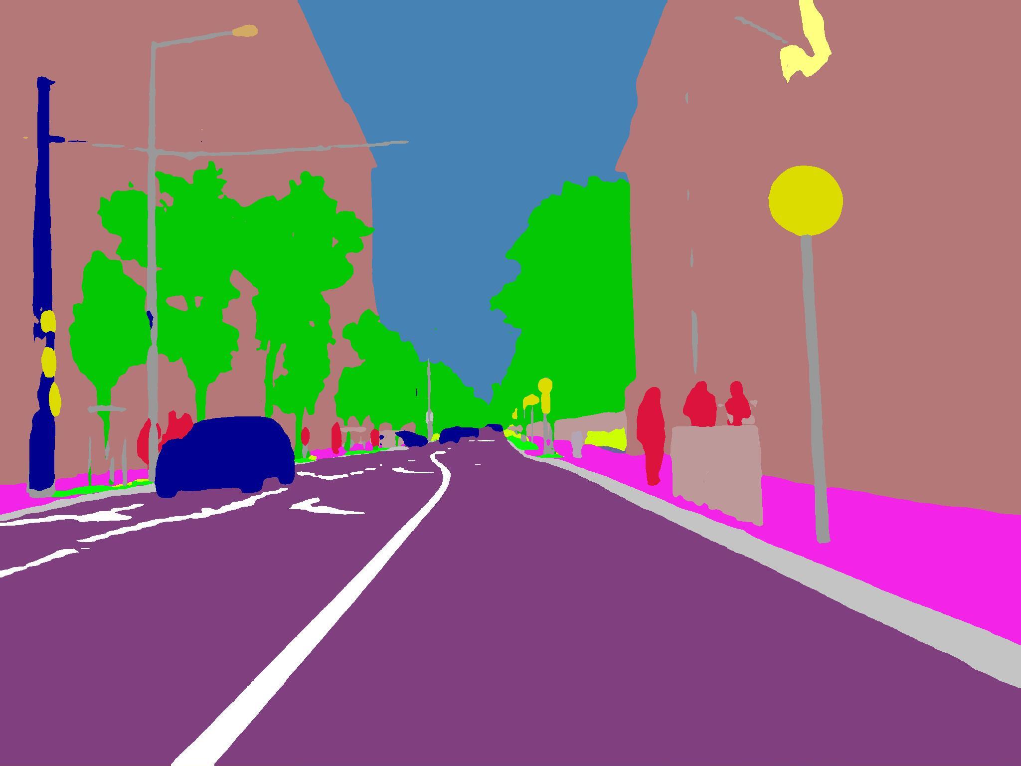
Figure 4 shows predictions of universal classes which correspond to the class road in Cityscapes test. Formally, the set of all such classes corresponds to $m_{\mathbbmsl{S}_{\mathrm{CS}}}(\mathrm{CS-road})$. These universal classes are: road, bike lane, crosswalk, zebra, road marking, pothole, manhole and service lane. No instance of pothole was found in the entire Cityscapes test. The best performing classes are road and road marking. We observe recognition of zebras only at close range, while otherwise they often get classified as road marking. The remaining classes are usually detected as small clusters in the correct region. For example, manholes are often only partially segmented.

Figure 4: Qualitative performance of our universal SNp-DN161 model on Cityscapes test. We overlay predictions over the input images. We show predictions of following universal classes: road (purple, all images), bike lane (yellow, top-left), crosswalk (red, top-left), zebra (green, top-right), road marking (white, all images), manhole (magenta, bottom-left) and service lane (lemon yellow, bottom-right).

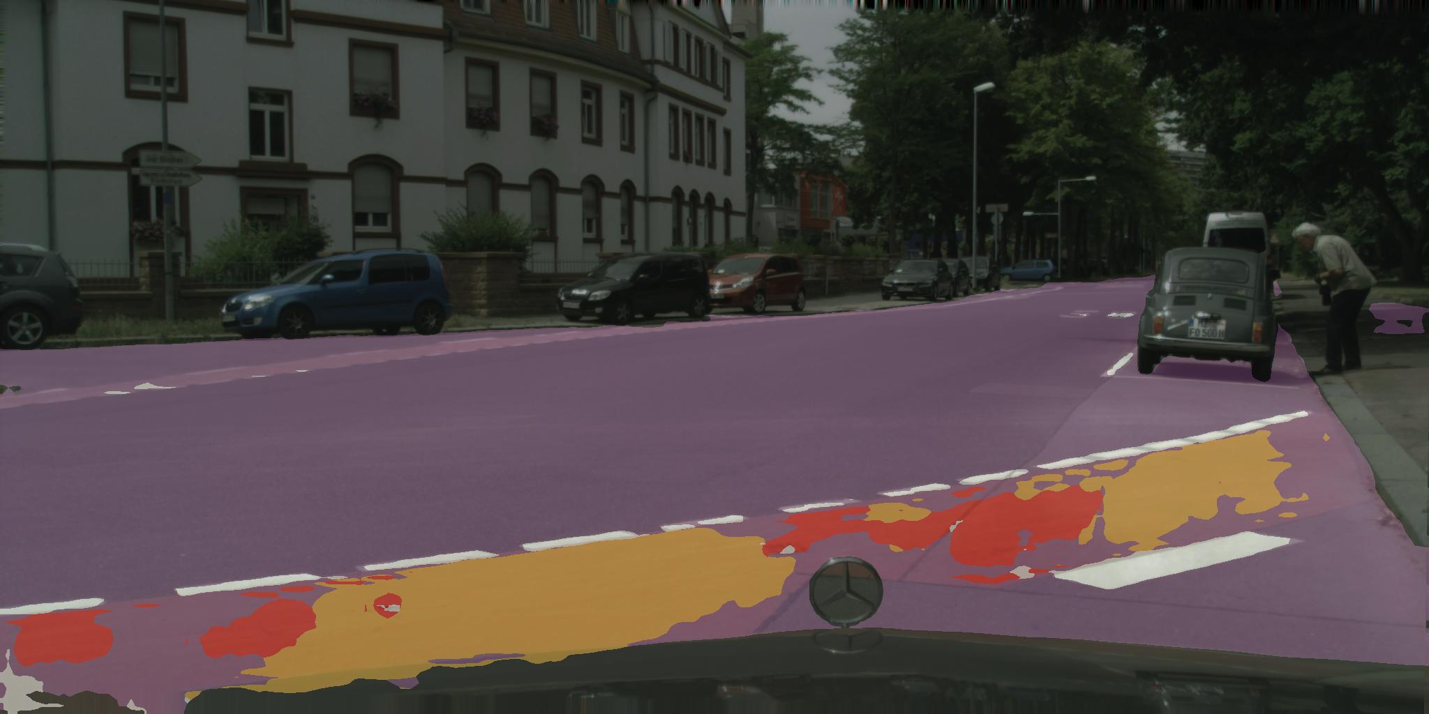
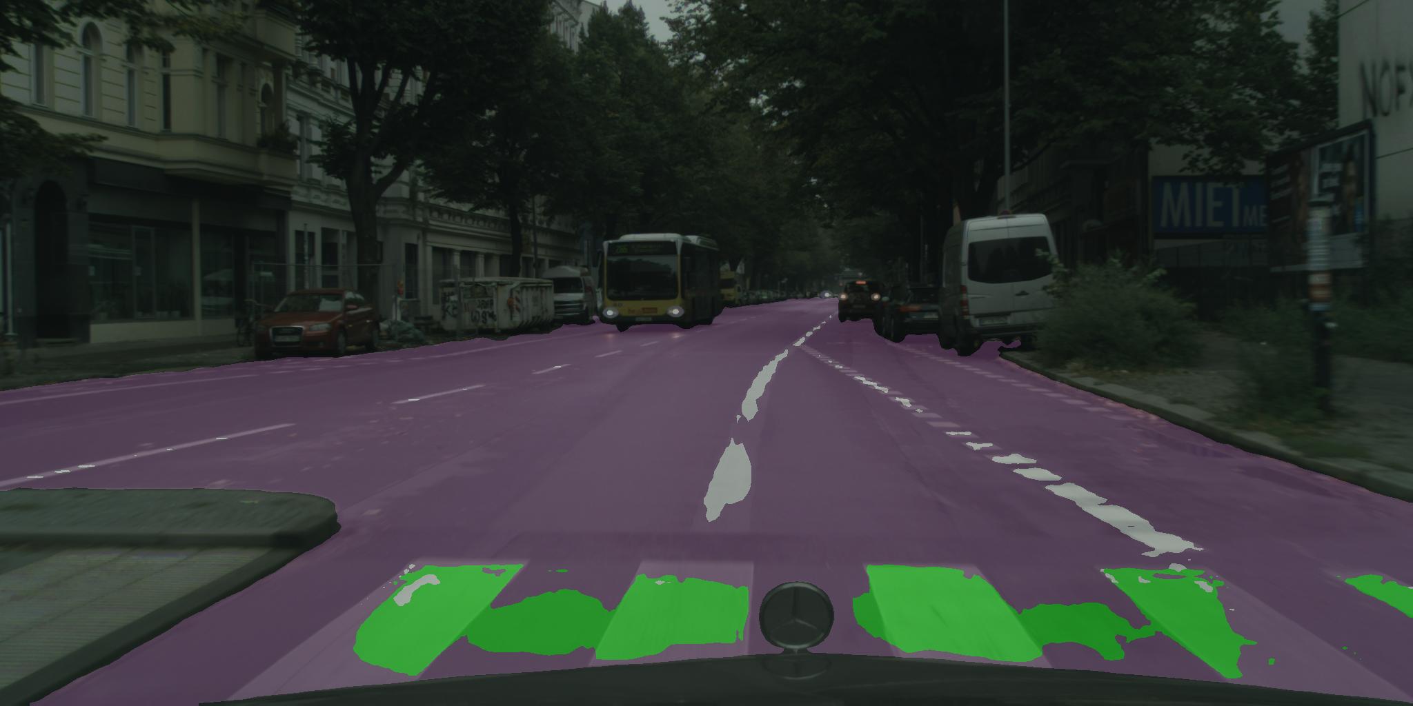
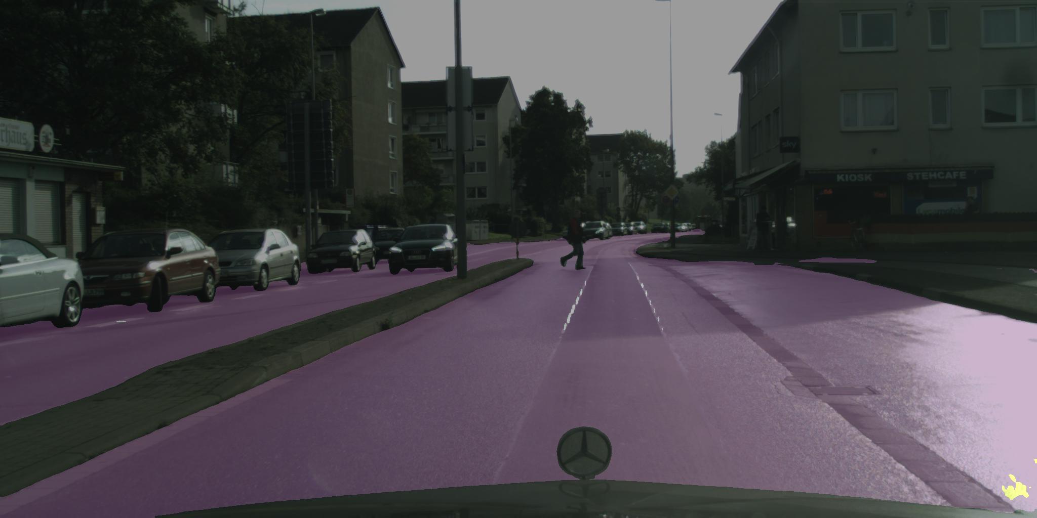
Figure 5 shows the performance of our model on negative images from WildDash. These images were taken in non-road driving contexts (rows 1-4) or from an unusual perspective (row 5). These images may contain classes found in traffic scenes such as people (row 2). Note that the benchmark accepts either the best-case ground truth or the void class (denoted with black).

Figure 5: Performance of our universal model on four WildDash 2 negative test images. The columns show the input image, universal segmentation, and the segmentation in the WildDash label space where class void is shown in black. Our model successfully recognizes some non-traffic classes, e.g. table, chair, book, and cabinet (row 2), or boat and water (row 5). The model is robust to perspective changes (row 5) and exhibits fair performance in presence of large domain-shift (row 3).

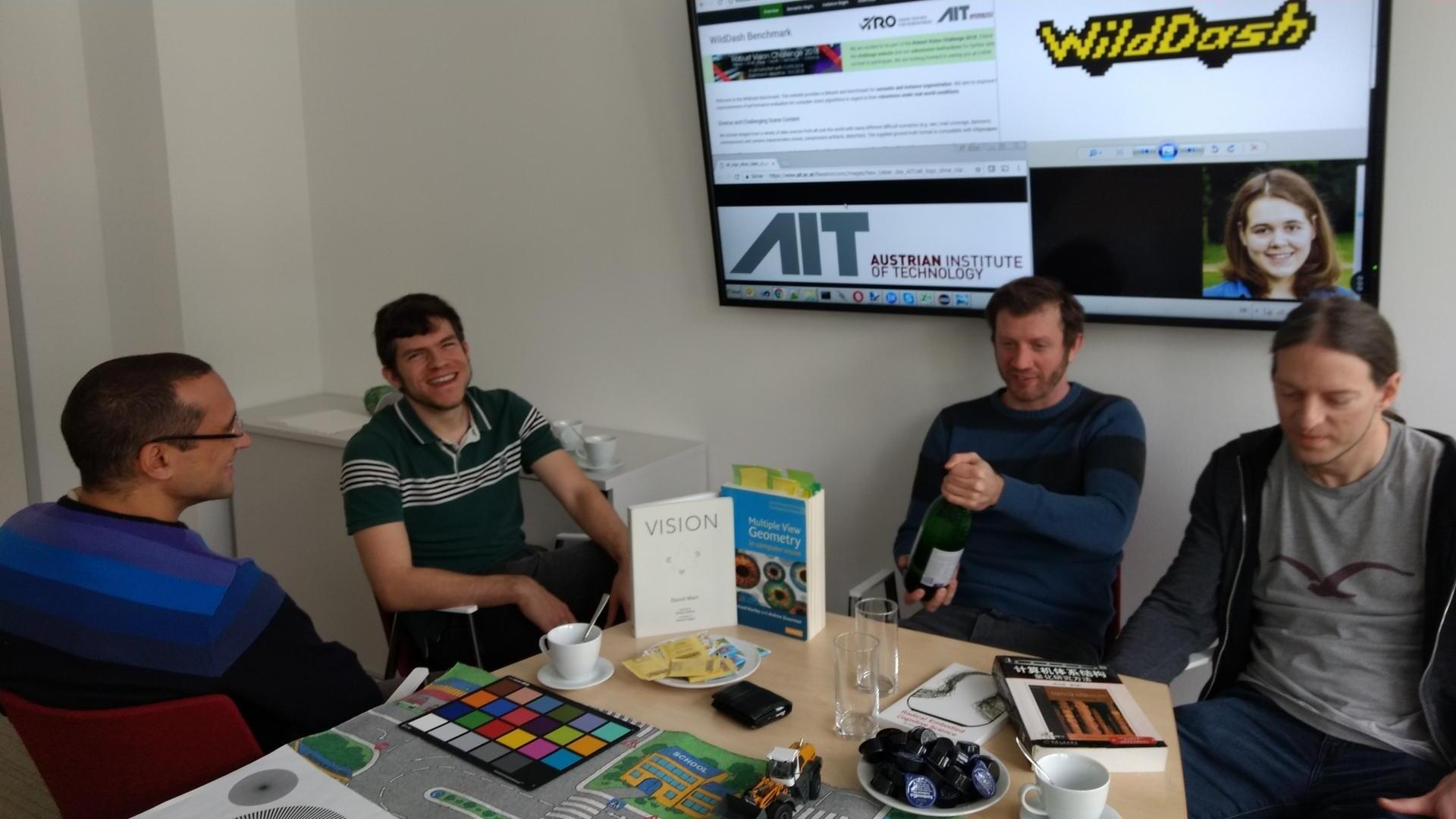
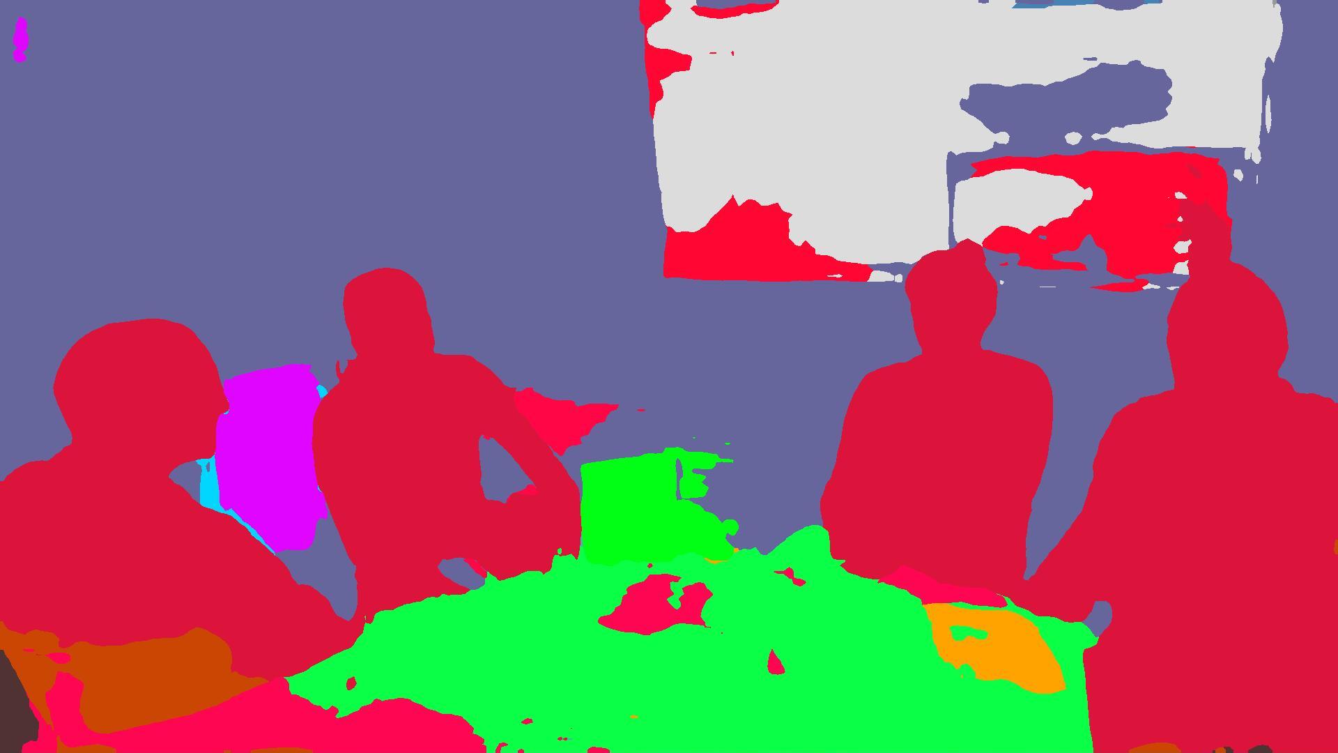
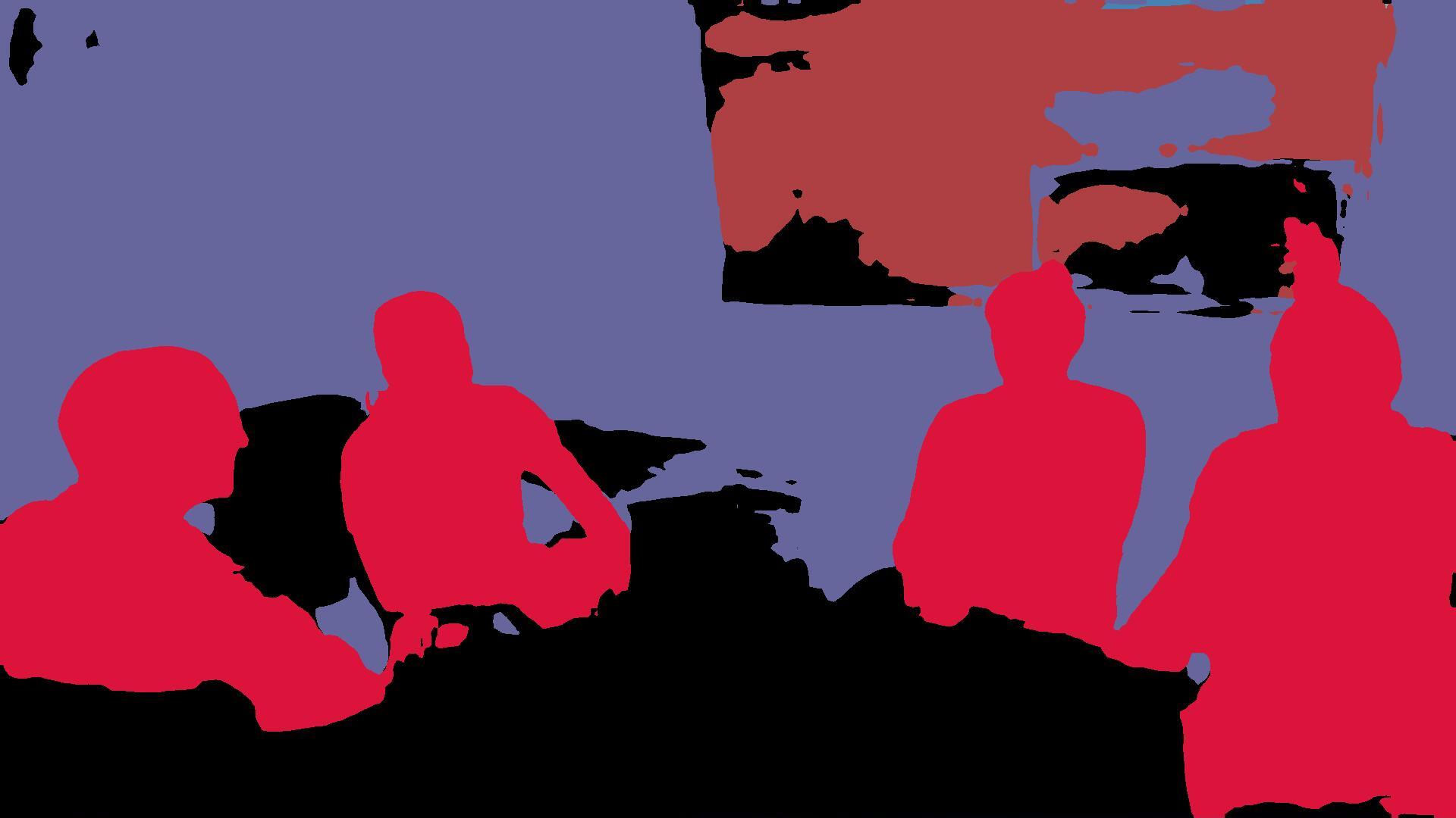
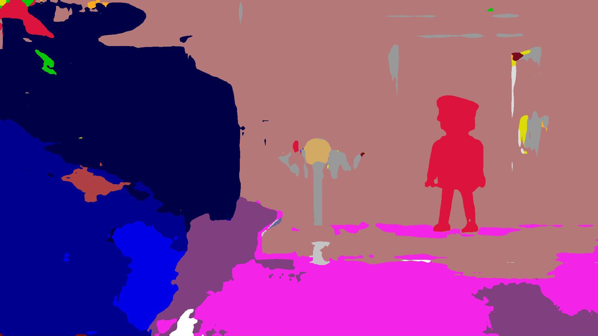
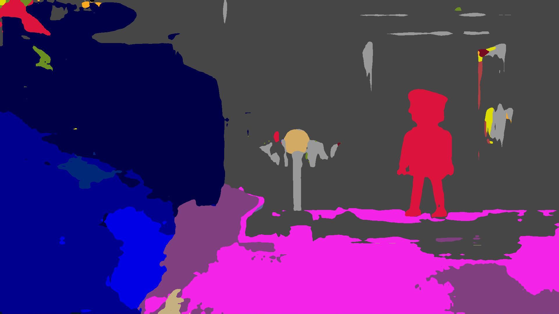
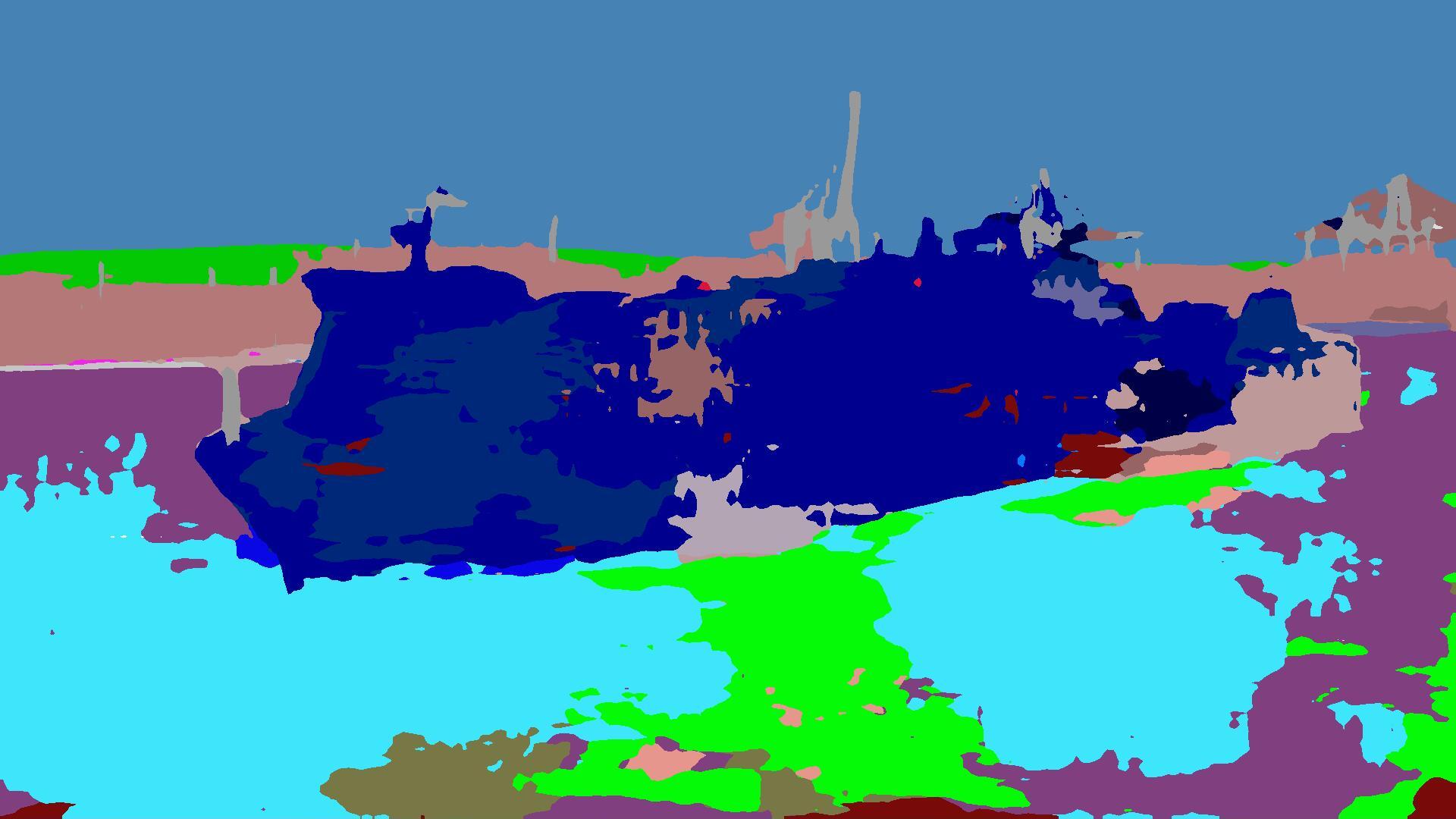
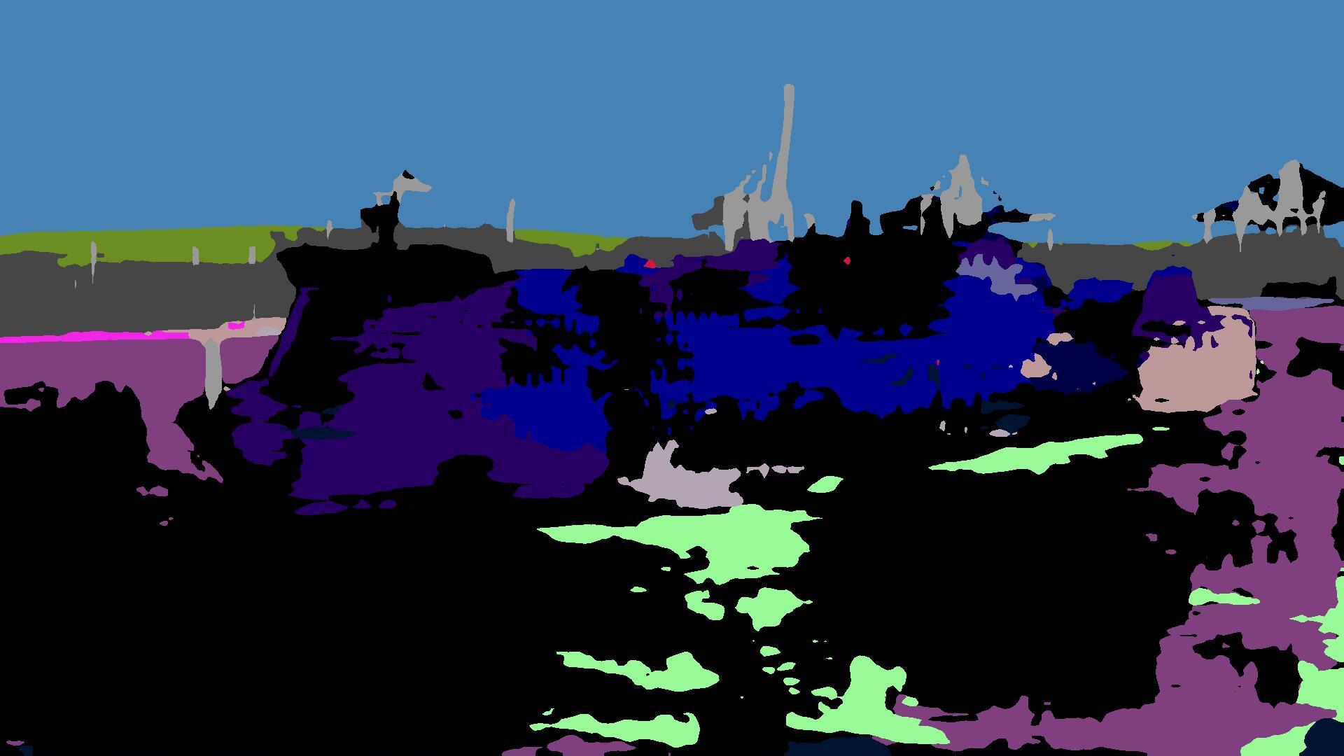
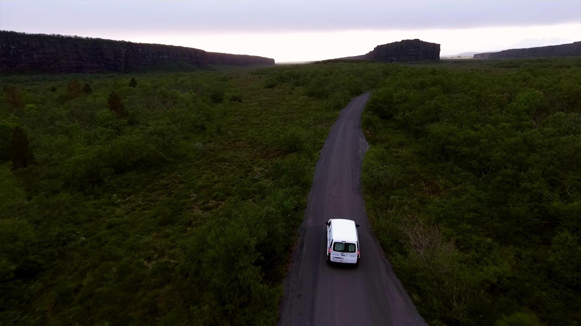
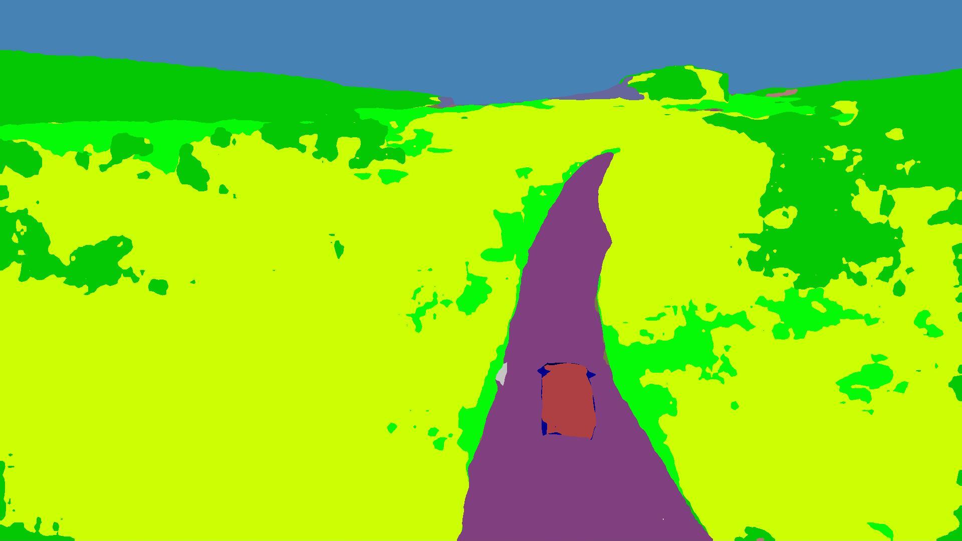
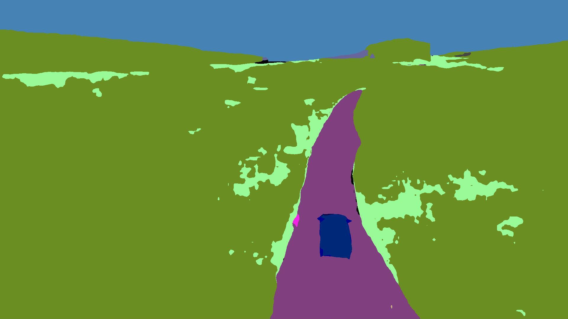
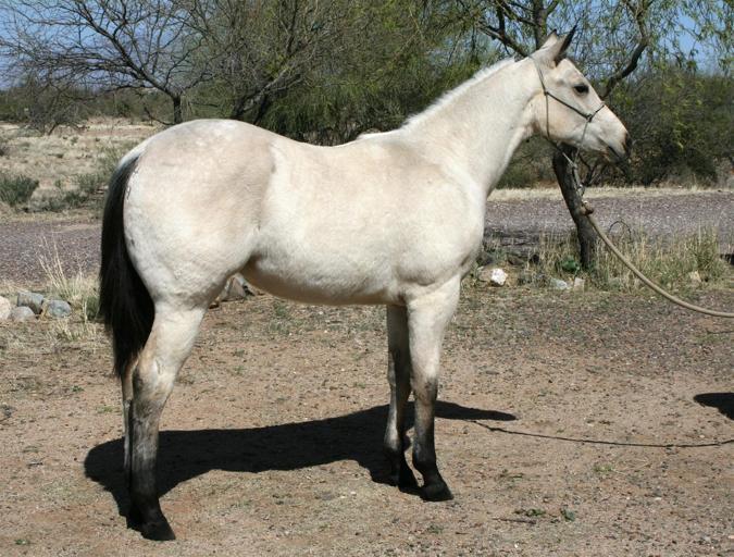
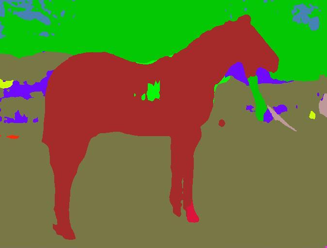
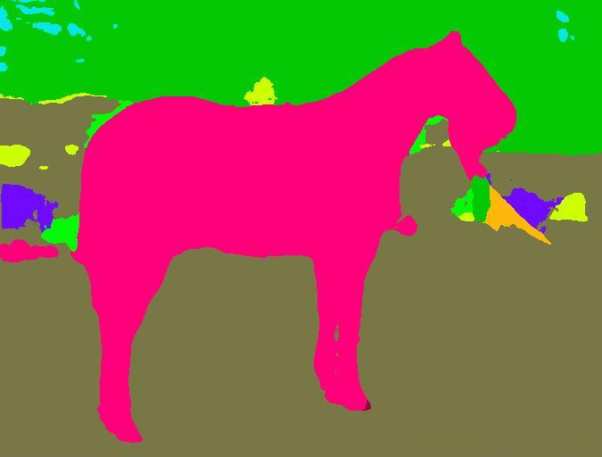
Figure 6 shows an interesting failure of our model to distinguish between different types of animals. Our universal model classifies the horse from an ADE20k image as class bird. This occurs since ADE20k taxonomy contains only the class animal which we map to universal classes bird and ground-animal. The training signal for distinguishing between birds and ground animals should have come from Vistas, but this signal was very weak since these two Vistas classes are extremely rare.

Figure 6: A failure case on ADE20k test. The columns show the input image, universal segmentation, and ADE20k segmentation. The model recognizes most of the horse as class bird. This occurs since birds and ground animals are annotated only in Vistas as extremely rare classes. Note that two patches are incorrectly classified as grass (green) and pedestrian (red). These patches finaly get correctly classified into ADE20k-animal, since the sum of probabilities of classes bird and ground animal prevails after evaluation mapping.

Appendix D Mapping visualizations

Figures 7 and 8 visualize training and evaluation mappings used in our City-Vistas experiments. We show these mappings for the two baselines and our universal taxonomy. Please refer to Section 3 of the main paper for a detailed description of the procedure for recovering these mappings.

(a)

(b)

(c)

Figure 7: Visualizations of training mappings in City-Vistas experiments. Naive concatenation (a) maps each dataset-specific class to the corresponding training logit. Partial merge (b) maps dataset-specific classes to the common logit only if they match exactly. If this is not the case, the classes remain separate. Our universal taxonomy (c) maps each dataset-specific class to one or more universal classes.

(a)

(b)

(c)

Figure 8: Visualizations of evaluation mappings in City-Vistas experiments for naive concatenation (a), partial merge (b) and universal taxonomy (c). In each of these cases, dataset-specific classes are mapped to training classes with which they overlap. We extend dataset-specific taxonomies with a void class that maps to all training classes which do not overlap with any of dataset-specific classes.

References

- [1] Vijay Badrinarayanan, Alex Kendall, and Roberto Cipolla. Segnet: A deep convolutional encoder-decoder architecture for image segmentation. IEEE Trans. Pattern Anal. Mach. Intell., 39(12):2481–2495, 2017.
- [2] Ping Chao, Chao-Yang Kao, Yu-Shan Ruan, Chien-Hsiang Huang, and Youn-Long Lin. Hardnet: A low memory traffic network. In ICCV, pages 3551–3560, 2019.
- [3] Liang-Chieh Chen, George Papandreou, Iasonas Kokkinos, Kevin Murphy, and Alan L Yuille. Deeplab: Semantic image segmentation with deep convolutional nets, atrous convolution, and fully connected crfs. IEEE transactions on pattern analysis and machine intelligence, 40(4):834–848, 2017.
- [4] Bowen Cheng, Maxwell D Collins, Yukun Zhu, Ting Liu, Thomas S Huang, Hartwig Adam, and Liang-Chieh Chen. Panoptic-deeplab: A simple, strong, and fast baseline for bottom-up panoptic segmentation. In Proceedings of the IEEE/CVF Conference on Computer Vision and Pattern Recognition, pages 12475–12485, 2020.
- [5] Marius Cordts, Mohamed Omran, Sebastian Ramos, Timo Rehfeld, Markus Enzweiler, Rodrigo Benenson, Uwe Franke, Stefan Roth, and Bernt Schiele. The cityscapes dataset for semantic urban scene understanding. In Proceedings of the IEEE conference on computer vision and pattern recognition, pages 3213–3223, 2016.
- [6] Timothee Cour, Ben Sapp, and Ben Taskar. Learning from partial labels. The Journal of Machine Learning Research, 12:1501–1536, 2011.
- [7] Angela Dai, Angel X. Chang, Manolis Savva, Maciej Halber, Thomas Funkhouser, and Matthias Nießner. Scannet: Richly-annotated 3d reconstructions of indoor scenes. In CVPR, 2017.
- [8] Andreas Geiger, Philip Lenz, Christoph Stiller, and Raquel Urtasun. Vision meets robotics: The kitti dataset. Int. J. Robotics Res., 32(11):1231–1237, 2013.
- [9] Kaiming He, Xiangyu Zhang, Shaoqing Ren, and Jian Sun. Deep residual learning for image recognition. In Proceedings of the IEEE conference on computer vision and pattern recognition, pages 770–778, 2016.
- [10] Yuanduo Hong, Huihui Pan, Weichao Sun, and Yisong Jia. Deep dual-resolution networks for real-time and accurate semantic segmentation of road scenes. CoRR, abs/2101.06085, 2021.
- [11] Gao Huang, Zhuang Liu, Geoff Pleiss, Laurens Van Der Maaten, and Kilian Weinberger. Convolutional networks with dense connectivity. IEEE transactions on pattern analysis and machine intelligence, 2019.
- [12] Tarun Kalluri, Girish Varma, Manmohan Chandraker, and CV Jawahar. Universal semi-supervised semantic segmentation. In Proceedings of the IEEE International Conference on Computer Vision, pages 5259–5270, 2019.
- [13] Ivan Kreso, Josip Krapac, and Sinisa Segvic. Ladder-style densenets for semantic segmentation of large natural images. In ICCV CVRSUAD, pages 238–245, 2017.
- [14] Ivan Krešo, Josip Krapac, and Siniša Šegvić. Efficient ladder-style densenets for semantic segmentation of large images. IEEE Transactions on Intelligent Transportation Systems, 2020.
- [15] John Lambert, Zhuang Liu, Ozan Sener, James Hays, and Vladlen Koltun. Mseg: A composite dataset for multi-domain semantic segmentation. In CVPR, 2020.
- [16] Xiaodan Liang, Hongfei Zhou, and Eric Xing. Dynamic-structured semantic propagation network. In CVPR, pages 752–761, 2018.
- [17] Tsung-Yi Lin, Michael Maire, Serge J. Belongie, James Hays, Pietro Perona, Deva Ramanan, Piotr Dollár, and C. Lawrence Zitnick. Microsoft COCO: common objects in context. In ECCV, pages 740–755, 2014.
- [18] Tsung-Yi Lin, Piotr Dollár, Ross Girshick, Kaiming He, Bharath Hariharan, and Serge Belongie. Feature pyramid networks for object detection. In Proceedings of the IEEE conference on computer vision and pattern recognition, pages 2117–2125, 2017.
- [19] Jonathan Long, Evan Shelhamer, and Trevor Darrell. Fully convolutional networks for semantic segmentation. In Proceedings of the IEEE conference on computer vision and pattern recognition, pages 3431–3440, 2015.
- [20] Panagiotis Meletis and Gijs Dubbelman. Training of convolutional networks on multiple heterogeneous datasets for street scene semantic segmentation. In Intelligent Vehicles Symposium, pages 1045–1050, 2018.
- [21] Gerhard Neuhold, Tobias Ollmann, Samuel Rota Bulò, and Peter Kontschieder. Mapillary vistas dataset for semantic understanding of street scenes. In ICCV, pages 5000–5009, 2017.
- [22] Dong Nie, Jia Xue, and Xiaofeng Ren. Bidirectional pyramid networks for semantic segmentation. In ACCV, pages 654–671, 2020.
- [23] Marin Orsic, Petra Bevandic, Ivan Grubisic, Josip Saric, and Sinisa Segvic. Multi-domain semantic segmentation with pyramidal fusion. arXiv preprint arXiv:2009.01636, 2020.
- [24] Marin Oršić and Siniša Šegvić. Efficient semantic segmentation with pyramidal fusion. Pattern Recognition, page 107611, 2021.
- [25] Lorenzo Porzi, Samuel Rota Bulò, Aleksander Colovic, and Peter Kontschieder. Seamless scene segmentation. In CVPR, pages 8277–8286, 2019.
- [26] Stephan R. Richter, Zeeshan Hayder, and Vladlen Koltun. Playing for benchmarks. In ICCV, pages 2232–2241, 2017.
- [27] Olaf Ronneberger, Philipp Fischer, and Thomas Brox. U-net: Convolutional networks for biomedical image segmentation. In International Conference on Medical image computing and computer-assisted intervention, pages 234–241. Springer, 2015.
- [28] Samuel Rota Bulò, Lorenzo Porzi, and Peter Kontschieder. In-place activated batchnorm for memory-optimized training of dnns. In Proceedings of the IEEE Conference on Computer Vision and Pattern Recognition, pages 5639–5647, 2018.
- [29] Roy Schwartz, Jesse Dodge, Noah A. Smith, and Oren Etzioni. Green AI. Commun. ACM, 63(12):54–63, 2020.
- [30] Shuran Song, Samuel P. Lichtenberg, and Jianxiong Xiao. Sun rgb-d: A rgb-d scene understanding benchmark suite. In CVPR, pages 567–576, 2015.
- [31] Chen Sun, Abhinav Shrivastava, Saurabh Singh, and Abhinav Gupta. Revisiting unreasonable effectiveness of data in deep learning era. In IEEE International Conference on Computer Vision, ICCV 2017, Venice, Italy, October 22-29, 2017, pages 843–852. IEEE Computer Society, 2017.
- [32] Girish Varma, Anbumani Subramanian, Anoop M. Namboodiri, Manmohan Chandraker, and C. V. Jawahar. IDD: A dataset for exploring problems of autonomous navigation in unconstrained environments. In WACV, pages 1743–1751, 2019.
- [33] Jingdong Wang, Ke Sun, Tianheng Cheng, Borui Jiang, Chaorui Deng, Yang Zhao, Dong Liu, Yadong Mu, Mingkui Tan, Xinggang Wang, Wenyu Liu, and Bin Xiao. Deep high-resolution representation learning for visual recognition. IEEE Transactions on Pattern Recognition and Machine Intelligence, 2020.
- [34] Fisher Yu, Wenqi Xian, Yingying Chen, Fangchen Liu, Mike Liao, Vashisht Madhavan, and Trevor Darrell. BDD100K: A diverse driving video database with scalable annotation tooling. arXiv preprint arXiv:1805.04687, 2018.
- [35] Yuhui Yuan, Xilin Chen, and Jingdong Wang. Object-contextual representations for semantic segmentation. In ECCV, 2020.
- [36] Oliver Zendel, Katrin Honauer, Markus Murschitz, Daniel Steininger, and Gustavo Fernandez Dominguez. Wilddash - creating hazard-aware benchmarks. In ECCV, 2018.
- [37] Chiyuan Zhang, Samy Bengio, Moritz Hardt, Benjamin Recht, and Oriol Vinyals. Understanding deep learning requires rethinking generalization. In 5th International Conference on Learning Representations, ICLR 2017, Toulon, France, April 24-26, 2017, Conference Track Proceedings. OpenReview.net, 2017.
- [38] Hengshuang Zhao, Xiaojuan Qi, Xiaoyong Shen, Jianping Shi, and Jiaya Jia. Icnet for real-time semantic segmentation on high-resolution images. In Vittorio Ferrari, Martial Hebert, Cristian Sminchisescu, and Yair Weiss, editors, Computer Vision - ECCV 2018 - 15th European Conference, Munich, Germany, September 8-14, 2018, Proceedings, Part III, volume 11207 of Lecture Notes in Computer Science, pages 418–434. Springer, 2018.
- [39] Hengshuang Zhao, Jianping Shi, Xiaojuan Qi, Xiaogang Wang, and Jiaya Jia. Pyramid scene parsing network. In Proceedings of the IEEE conference on computer vision and pattern recognition, pages 2881–2890, 2017.
- [40] Xiangyun Zhao, Samuel Schulter, Gaurav Sharma, Yi-Hsuan Tsai, Manmohan Chandraker, and Ying Wu. Object detection with a unified label space from multiple datasets. In ECCV, pages 178–193, 2020.
- [41] Bolei Zhou, Hang Zhao, Xavier Puig, Sanja Fidler, Adela Barriuso, and Antonio Torralba. Scene parsing through ade20k dataset. In CVPR, pages 633–641, 2017.
- [42] Yi Zhu, Karan Sapra, Fitsum A Reda, Kevin J Shih, Shawn Newsam, Andrew Tao, and Bryan Catanzaro. Improving semantic segmentation via video propagation and label relaxation. In Proceedings of the IEEE Conference on Computer Vision and Pattern Recognition, pages 8856–8865, 2019.
- [43] Aleksandar Zlateski, Ronnachai Jaroensri, Prafull Sharma, and Frédo Durand. On the importance of label quality for semantic segmentation. In CVPR, pages 1479–1487, 2018.