Abstract

Mixture of regression models are useful for regression analysis in heterogeneous populations where a single regression model may not be appropriate for the entire population. We study the nonparametric maximum likelihood estimator (NPMLE) for fitting these models. The NPMLE is based on convex optimization and does not require prior specification of the number of mixture components. We establish existence of the NPMLE and prove finite-sample parametric (up to logarithmic multiplicative factors) Hellinger error bounds for the predicted density functions. We also provide an effective procedure for computing the NPMLE without ad-hoc discretization and prove a theoretical convergence rate under certain assumptions. Numerical experiments on simulated data for both discrete and non-discrete mixing distributions demonstrate the remarkable performances of our approach. We also illustrate the approach on two real datasets.
Keywords: conditional gradient method, empirical Bayes, finite-sample parametric rate, Hellinger distance, mixture of regression, nonparametric maximum likelihood estimator (NPMLE), random coefficient regression.

1 Introduction

Given a univariate response variable $Y$ and a $p$-dimensional regressor variable $X$, the usual linear regression model with homoscedastic Gaussian errors assumes that the conditional distribution of $Y$ given $X=x$ is normal with mean $x^{\top}\beta$ and variance $\sigma^{2}$ for some $\beta\in\mathbb{R}^{p}$ and $\sigma>0$. In other words, the conditional density of $Y|X=x$ is given by

$$y\mapsto\frac{1}{\sigma}\phi\left(\frac{y-x^{\top}\beta}{\sigma}\right),$$

where $\phi$ denotes the standard normal density function. In contrast, the mixture of linear regression model assumes that the conditional density of $Y$ given $X=x$ is the mixture density

$$y\mapsto f_{x}^{G^{*}}(y):=\int\frac{1}{\sigma}\phi\left(\frac{y-x^{\top}\beta}{\sigma}\right)dG^{*}(\beta)$$

for some probability measure $G^{*}$ on $\mathbb{R}^{p}$ and $\sigma>0$. Equivalently, given $X=x$, the mixture of linear regression model can be written as

$$Y=x^{\top}\beta+\sigma Z\qquad\text{where $\beta\sim G^{*}$ and $Z\sim N(0,1)$ are independent,}$$ (1)

and $N(0,1)$ denotes the standard normal distribution.

The mixture of linear regression model is a prominent mixture model in statistics and machine learning and has a long history (see, for example, Quandt (1958); De Veaux (1989); Jordan and Jacobs (1994); Faria and Soromenho (2010)). It offers a simple approach to modeling population heterogeneity which is present in many real-world applications of linear regression. For example, in pharmacokinetics, different subjects react to drug treatments differently and, in marketing, different consumers have different drivers of satisfaction. As a result, mixture of regression models have been applied in diverse fields including biology (Martin-Magniette et al. (2008)), economics (Battisti and De Vaio (2008)), engineering (Liem et al. (2015)), epidemiology (Turner (2000)), marketing (Wedel and Kamakura (2012); Sarstedt (2008)), and traffic modeling (Elhenawy et al. (2016)). Because of the assumption that the regression parameters are random, mixture of regression models are also known as random coefficient regression models (Hildreth and Houck (1968); Longford (1994); Beran and Millar (1994); Beran and Hall (1992); Beran et al. (1996)).

Suppose we observe $n$ independent observations $(x_{1},y_{1}),\dots,(x_{n},y_{n})$ from the model (1), i.e.,

$$y_{i}=x_{i}^{\top}\beta^{i}+\sigma z_{i}\qquad\text{for $i=1,\dots,n$}$$ (2)

where $\beta^{1},\dots,\beta^{n},z_{1},\dots,z_{n}$ are independent with

$$\beta^{1},\dots,\beta^{n}\overset{\text{i.i.d.}}{\sim}G^{*}\text{ and }z_{1},\dots,z_{n}\overset{\text{i.i.d.}}{\sim}N(0,1).$$ (3)

If $\sigma$ and $G^{*}$ are known, the above can be seen as a Bayesian model with parameters $\beta^{i},i=1,\dots,n$, and one can perform individual inference on each regression coefficient $\beta^{i}$ via its posterior distribution. The posterior distribution for $\beta^{i}$, given the data point $(x_{i},y_{i})$, will be absolutely continuous with respect to the prior $G^{*}$ and have density proportional to $\phi((y_{i}-x_{i}^{\top}\beta)/\sigma)$:

$$\mathbb{P}\left\{\beta^{i}\in A\mid x_{i},y_{i}\right\}=\frac{\int_{A}\frac{1}{\sigma}\phi\left(\frac{y_{i}-x_{i}^{\top}\beta}{\sigma}\right)dG^{*}(\beta)}{\int\frac{1}{\sigma}\phi\left(\frac{y_{i}-x_{i}^{\top}\beta}{\sigma}\right)dG^{*}(\beta)}$$ (4)

for subsets $A\subseteq\mathbb{R}^{p}$. This posterior distribution can be used to do individual inference on each parameter $\beta^{i}$ separately for $i=1,\dots,n$. One can summarize this into point estimates for $\beta^{i}$ in the usual way by taking, for example, the posterior mean:

$$\hat{\beta}^{i}_{\mathrm{OB}}:=\mathbb{E}\left(\beta^{i}\mid x_{i},y_{i}\right)=\frac{\int_{A}\frac{1}{\sigma}\phi\left(\frac{y_{i}-x_{i}^{\top}\beta}{\sigma}\right)\beta dG^{*}(\beta)}{\int\frac{1}{\sigma}\phi\left(\frac{y_{i}-x_{i}^{\top}\beta}{\sigma}\right)dG^{*}(\beta)}.$$ (5)

The subscript OB in $\hat{\beta}^{i}_{\mathrm{OB}}$ stands for “Oracle Bayes”; Oracle here is used to refer to the fact that $G^{*}$ is typically unknown and thus known only to an Oracle.

This ability to do individual inference on the regression coefficient $\beta^{i}$ corresponding to each separate data point $(x_{i},y_{i})$ is the main attractive feature of the mixture of linear regression model. This would, of course, require knowledge of $G^{*}$ (as well as $\sigma$). The goal of this paper is to study the problem of estimating $G^{*}$ from the data $(x_{1},y_{1}),\dots,(x_{n},y_{n})$. We shall assume for most of the paper that $\sigma$ is known. In practice, it is easy to estimate $\sigma$ by $\hat{\sigma}$ using a simple cross-validation procedure as described in Subsection 4.1. If $G^{*}$ is estimated by, say, a discrete probability measure $\hat{G}:=\sum_{j=1}^{\hat{k}}\hat{\pi}_{j}\delta_{\{\hat{\beta}_{j}\}}$, then the posterior distribution given by (4) will be estimated by the discrete probability distribution:

$$\sum_{j=1}^{\hat{k}}\left[\frac{\hat{\pi}_{j}\phi\left(\frac{y_{i}-x_{i}^{\top}\hat{\beta}_{j}}{\hat{\sigma}}\right)}{\sum_{l=1}^{\hat{k}}\hat{\pi}_{l}\phi\left(\frac{y_{i}-x_{i}^{\top}\hat{\beta}_{l}}{\hat{\sigma}}\right)}\right]\delta_{\{\hat{\beta}_{j}\}}\qquad\text{for $j=1,\dots,\hat{k}$}$$ (6)

and the posterior mean (5) will be estimated by

$$\hat{\beta}^{i}_{\mathrm{EB}}:=\frac{\sum_{l=1}^{\hat{k}}\hat{\beta}_{l}\hat{\pi}_{l}\phi\left(\frac{y_{i}-x_{i}^{\top}\hat{\beta}_{l}}{\hat{\sigma}}\right)}{\sum_{l=1}^{\hat{k}}\hat{\pi}_{l}\phi\left(\frac{y_{i}-x_{i}^{\top}\hat{\beta}_{l}}{\hat{\sigma}}\right)}.$$ (7)

These can be used for approximate individual inference for $\beta^{i},i=1,\dots,n$. The subscript $\mathrm{EB}$ in $\hat{\beta}^{i}_{\mathrm{EB}}$ stands for “Empirical Bayes”; Empirical here is used to refer to the fact that parameters $G^{*}$ and $\sigma$ are estimated from the data.

For estimation of $G^{*}$, most usual approaches assume a parametric form for $G^{*}$. For example, it is popular to assume that $G^{*}$ is a discrete probability measure with a known number $k$ of atoms and estimation is then done by maximum likelihood. Likelihood maximization in this case is a non-convex optimization problem and is typically carried out via the expectation maximization (EM) algorithm (see, for example, Leisch (2004); Faria and Soromenho (2010)). In contrast with this parametric approach, we take a nonparametric approach in this paper where we do not impose any parametric assumptions on $G^{*}$. However, like in the parametric case, we perform estimation of $G^{*}$ via maximum likelihood. We therefore follow the strategy of nonparametric maximum likelihood estimation for estimating $G^{*}$.

Nonparametric maximum likelihood estimation for mixture models has a very long history starting with Robbins (1950) and Kiefer and Wolfowitz (1956). Book-length treatments on NPMLEs are Lindsay (1995); Groeneboom and Wellner (1992); Böhning (2000) and Schlattmann (2009). There has been renewed interest in these methods more recently (Zhang (2009); Koenker and Mizera (2014); Dicker and Zhao (2016); Saha and Guntuboyina (2020); Gu and Koenker (2020); Jagabathula et al. (2020); Deb et al. (2021); Polyanskiy and Wu (2020)). Most of these papers focus on the problem of estimating normal mixture densities with the exception of Gu and Koenker (2020) which deals with mixture of binary regression and Jagabathula et al. (2020) which deals with mixture of logit models.

Let us now describe our estimator for $G^{*}$ more precisely assuming that $\sigma$ is known. The likelihood function in this model can be taken to be the conditional density of $y_{1},\dots,y_{n}$ given $x_{1},\dots,x_{n}$ and its logarithm (the log-likelihood function) is given by

$$G\mapsto\sum_{i=1}^{n}\log f_{x_{i}}^{G}(y_{i})\qquad\text{where $f^{G}_{x_{i}}(y_{i})=\frac{1}{\sigma}\int\phi\left(\frac{y_{i}-x_{i}^{\top}\beta}{\sigma}\right)dG(\beta),i=1,\dots,n.$}$$ (8)

A Nonparametric Maximum Likelihood Estimator (NPMLE) of $G^{*}$ is obtained by maximizing the log-likelihood function over a large class of probability measures $G$ on $\mathbb{R}^{p}$. It often makes sense to impose bounds on the support of $G$ in the maximization of the likelihood. As a result, we consider, for a given set $K\subseteq\mathbb{R}^{p}$, the estimator:

$$\hat{G}\in\mathop{\rm argmax}\left\{\sum_{i=1}^{n}\log f_{x_{i}}^{G}(y_{i}):G\text{ is a probability supported on }K\right\}$$ (9)

If no information about the support of $G^{*}$ is available, then one can either take $K$ to be the whole of $\mathbb{R}^{p}$ or a large compact set such as a closed ball centered at the origin having a large radius.

The optimization in (9) is infinite-dimensional as $K$ is usually uncountable. However it is a convex optimization problem as the constraint set (the set of all probability measures on $K$) is convex and the objective function is concave in $G$. We prove in Section 2 that $\hat{G}$ exists when $K$ is compact or when $K$ satisfies a technical condition which holds when $K=\mathbb{R}^{p}$. We also provide an iterative algorithm for computing an approximate solution $\hat{G}$ that is discrete. The algorithm is one of the variants of the Conditional Gradient Method (CGM) also known as the Frank-Wolfe algorithm (Frank and Wolfe (1956); Jaggi (2013)). This algorithm comes with convergence bounds which guarantee that the iterates converge to a global maximizer of the likelihood provided some conditions are satisfied. Even though these conditions seem difficult to verify in practice, we found that the algorithm works very well in a variety of simulation settings and real datasets. Our approach to computing the NPMLE based on the Conditional Gradient Method is very similar to the computational procedure of Jagabathula et al. (2020). The discrete estimate $\hat{G}$ which can be written as $\sum_{j=1}^{\hat{k}}\hat{\pi}_{j}\delta_{\{\hat{\beta}_{j}\}}$ can be used for individual inference on $\beta^{i}$ via (6) and (7).

The estimator $\hat{G}$ works well and does not suffer from overfitting even though it is obtained by maximization over a very large class of probability measures. To illustrate, consider the simulated dataset shown in Figure 1(a) where each data point is generated by adding $N(0,\sigma^{2})$ ($\sigma=0.5$) noise to one of the three lines: $3-x,1+1.5x,-1+0.5x$ chosen with probabilities $0.3,0.3,0.4$ (the design points are independently generated from the uniform distribution on $[-1,3]$). We visualize $G^{*}$ together with all data points in Figure 1(b), where each data point is color coded according to the line they are generated from. Of course, this color coding and the equations of the three generating lines are not part of the dataset and unavailable to the data analyst.

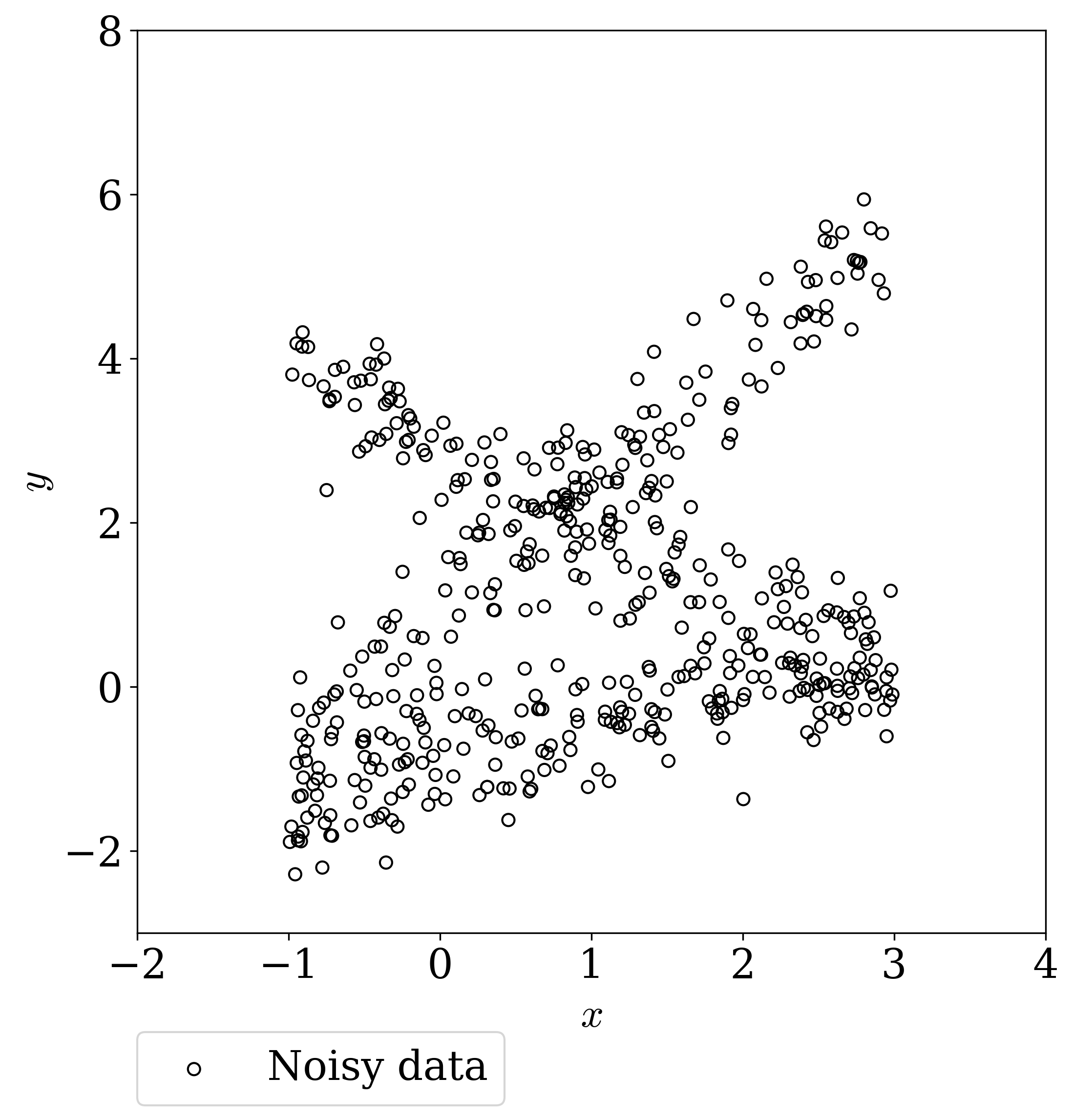
(a) Simulated dataset

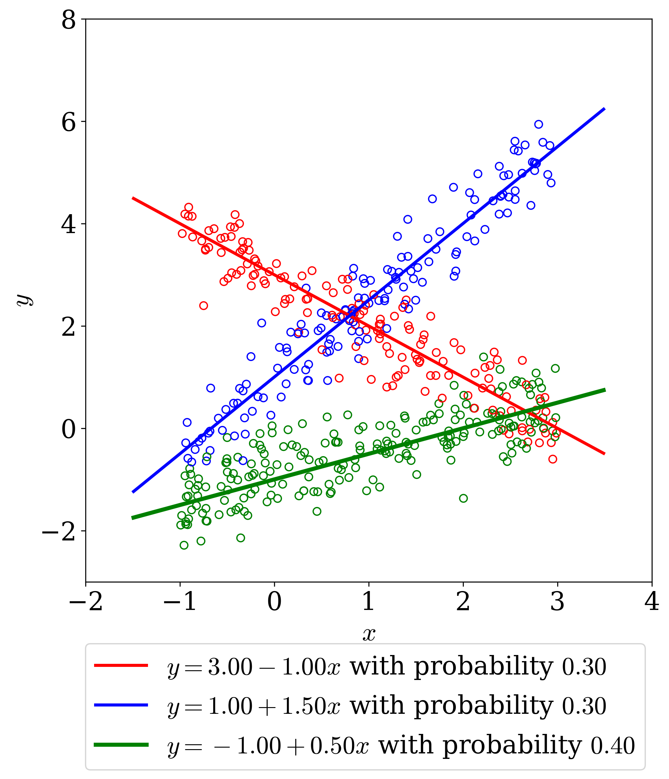
(b) True mixture

Figure 1: Simulated data from a three-component mixture of linear regression model: (a) Scatter plots of simulated dataset where $y$ represents noisy response and $x$ represents univariate covariate; (b) True regression components with each data point colored the same as its corresponding component.

A common way of analyzing this dataset is to first guess that the data is generated from a three-component mixture of linear regression model by eyeballing Figure 1(a) and then fit such a mixture via the EM algorithm. In contrast, our method does not make any such parametric assumptions.

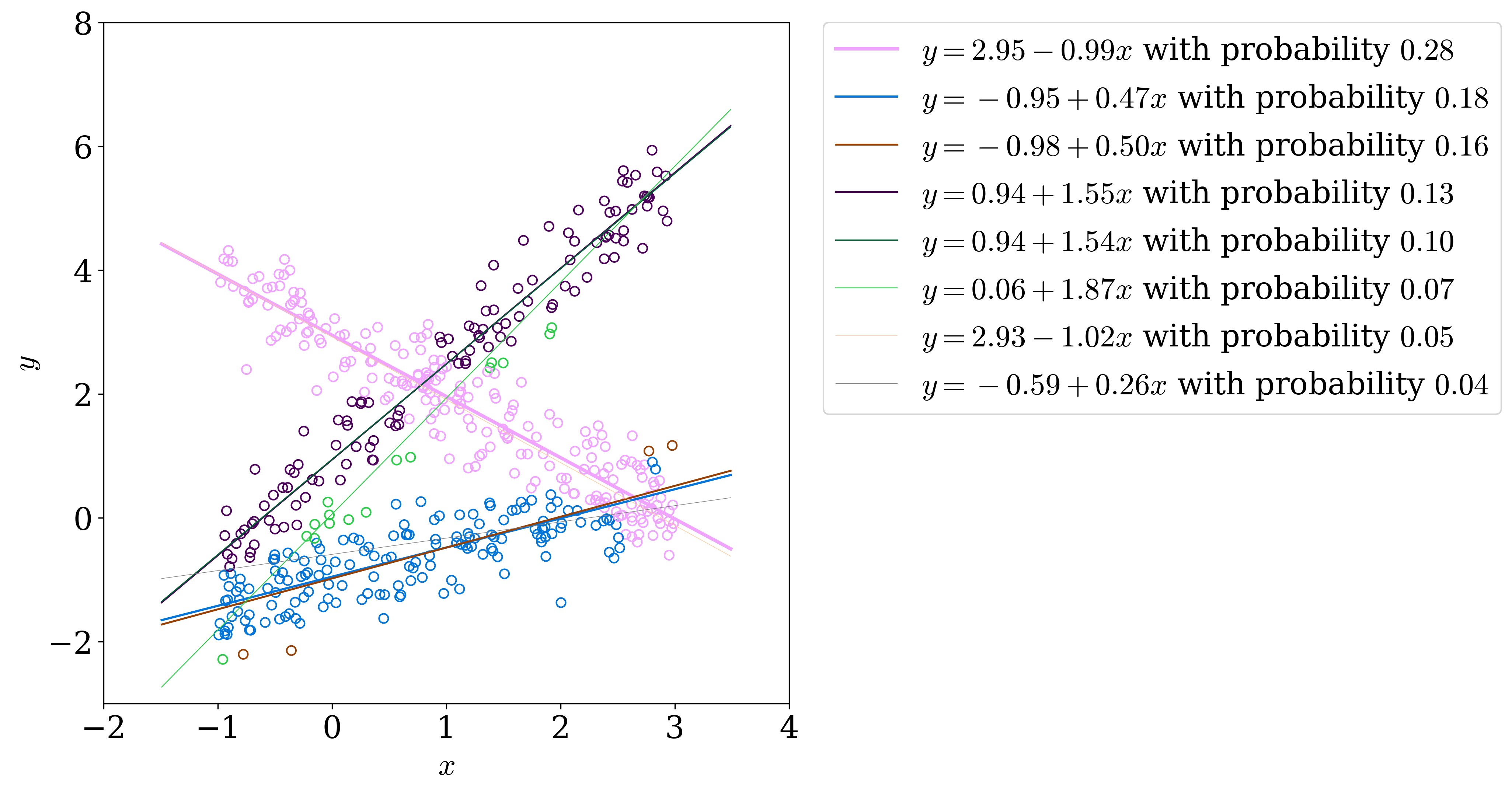
Figure 2: Fitted mixture by NPMLE approach with $\hat{\sigma}=0.48$ chosen by cross-validation. For comparison, the estimated components by EM initialized with true parameters are $y=2.9395-0.9934x$ with probability $0.33$, $y=-0.8473+1.5483x$ with probability $0.29$, $y=-0.9428+0.4754x$ with probability $0.38$.

For this dataset, we applied our procedure based on the NPMLE defined in (9) with $K=[-10,10]^{2}$ and $\hat{\sigma}=0.48$. The $\hat{\sigma}$ value was obtained by the cross-validation method described in Subsection 4.1, and it is rather close to $\sigma=0.5$. We use $\hat{G}_{\text{CV}}$ to represent the estimate via NPMLE with the $\hat{\sigma}$ by cross-validation, to distinguish from $\hat{G}$ via NPMLE with the true $\sigma$. Our algorithm outputted $\hat{G}_{\text{CV}}$ that is a discrete probability measure $\sum_{j=1}^{\hat{k}}\hat{\pi}_{j}\delta_{\{\hat{\beta}_{j}\}}$ supported on $\hat{k}=8$ points; the regression lines corresponding to the coefficients $\hat{\beta}_{j},1\leq j\leq 8$ of these 8 support points are displayed in Figure 2 (the thickness and darkness of each line is proportional to its estimated mixing probability). We colored the 8 different lines with 8 different colors and further colored each data point $(x_{i},y_{i})$ with the color of the regression line corresponding to the most probable posterior line:

$$\mathop{\rm argmax}_{1\leq j\leq\hat{k}}\left[\hat{\pi}_{j}\phi\left(\frac{y_{i}-x_{i}^{\top}\hat{\beta}_{j}}{\hat{\sigma}}\right)\right].$$ (10)

It is not surprising that the number of fitted regressions lines is larger than the true number 3 because the NPMLE is maximizing over a very large class of probability measures. However, critical structures of the three groups are recovered and, especially, each regression line with an estimated probability of at least $0.10$ is very close to one of the three true lines in Figure 1(b). Furthermore, the estimated conditional density function

$$(x,y)\mapsto f_{x}^{\hat{G}_{\text{CV}},\hat{\sigma}}(y):=\frac{1}{\hat{\sigma}}\int\phi\left((y_{i}-x_{i}^{\top}\beta)/\hat{\sigma}\right)d\hat{G}_{\text{CV}}(\beta)\displaystyle$$

is very close to the true conditional density function $(x,y)\mapsto f_{x}^{G^{*}}(y)$, and the accuracy is comparable to that of the density estimate given by the three-component EM algorithm initialized with true parameters:

$$(x,y)\mapsto f_{x}^{\hat{G}_{\text{EM}},\hat{\sigma}_{\text{EM}}}(y):=\frac{1}{\hat{\sigma}_{\text{EM}}}\int\phi\left((y_{i}-x_{i}^{\top}\beta)/\hat{\sigma}_{\text{EM}}\right)d\hat{G}_{\text{EM}}(\beta)\displaystyle,$$

and the estimate $(x,y)\mapsto f_{x}^{\hat{G}}(y)$ given by the NPMLE with the true $\sigma$ parameter. This is depicted in Figure 3.

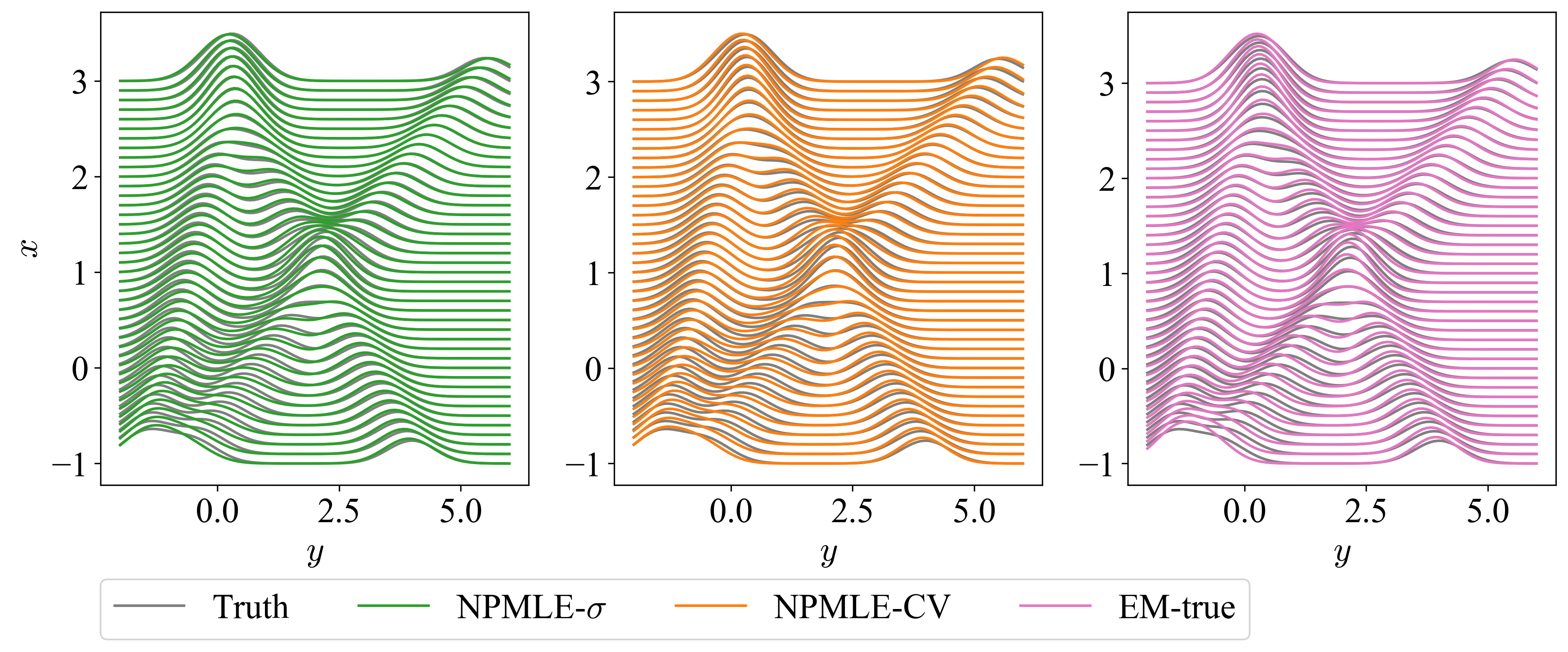
Figure 3: Ridgeline plots of density functions $f_{x}^{G^{*}}(y)$ in comparison with its estimates via (i) NPMLE-$\sigma$ (NPMLE with known $\sigma$), (ii) NPMLE-CV (NPMLE with $\hat{\sigma}$ selected by cross-validation), and (iii) EM-true (EM initialized with true parameters of $G^{*}$ and $\sigma$) respectively.

We have been able to prove rigorous results which show that the estimated conditional density function $(x,y)\mapsto f_{x}^{\hat{G}}(y)$ is a very good estimator for the true conditional density function $(x,y)\mapsto f_{x}^{G^{*}}(y)$ under general conditions on $G^{*}$ and assuming that $\sigma$ is known. These results are stated in terms of averaged squared Hellinger loss functions. For each fixed $x$, model (1) states that the conditional distribution of the response $Y$ given $X=x$ is $f_{x}^{G^{*}}(\cdot)$ which we estimate by $f_{x}^{\hat{G}}(\cdot)$. A natural and popular measure for comparing the discrepancy between the two densities $f_{x}^{G^{*}}(\cdot)$ and $f_{x}^{\hat{G}}(\cdot)$ is the squared Hellinger distance

$$\mathfrak{H}^{2}\left(f^{\hat{G}}_{x},f^{G^{*}}_{x}\right)=\int\left\{\sqrt{f^{\hat{G}}_{x}(y)}-\sqrt{f^{G^{*}}_{x}(y)}\right\}^{2}dy.$$ (11)

The squared Hellinger distance is a very popular loss function in density estimation (see, e.g., van de Geer (2000); Van Der Vaart and Wellner (1996)) and it has also been used in theoretical analysis of the NPMLE in Gaussian location mixture models (Ghosal and Van Der Vaart, 2001; Zhang, 2009; Saha and Guntuboyina, 2020).

The squared Hellinger distance in (11) is defined for a given $x$. To get an overall error function, it is natural to average over $x$. In the fixed design setting, we average over the observed design points $x_{1},\dots,x_{n}$ and in the random design setting, we average with respect to the distribution of $x$. Assuming that the set $K$ in (9) is a compact ball and that $G^{*}$ is supported on $K$, we prove that the averaged squared Hellinger distance is, with high probability, of order $n^{-1}$ up to multiplicative logarithmic factors in both the fixed design (Theorem 28) and random design (Theorem 4) settings. This proves the effectiveness of the fully nonparametric strategy of estimating $G^{*}$: one does not need to make any parametric assumptions on $G^{*}$ and, at the same time, achieves near parametric rates for conditional density estimation (in the case where $G^{*}$ is compactly supported).

In the random design setting, we also prove that $\hat{G}$ is consistent for $G^{*}$ in the sense that the Lévy-Prokhorov distance between $\hat{G}$ and $G^{*}$ converges to zero in probability as $n\rightarrow\infty$. This result (Theorem 5) also requires the assumption that the set $K$ in (9) is a compact ball and that $G^{*}$ is supported on $K$.

The remainder of this paper is organized as follows. In Section 2, we discuss the existence and computation of NPMLE. In Section 3, we present our theoretical results on the accuracy of the NPMLE. In Section 4, we provide experimental results including simulation studies and real data analysis. All these experimental results can be replicated with the code and data available at https://github.com/hanshengjiang/npmle_git. In Section 5, we argue that our methodology can also be used for the more general case of mixtures of nonlinear regression models. Proofs of all our theorems are given in Section 6.

2 Existence and Computation

2.1 Existence

We prove below that an NPMLE $\hat{G}$ defined as in (9) exists, assuming that $K$ is either compact or that it satisfies a technical condition that holds when $K$ is the whole space $\mathbb{R}^{p}$. The following notation is used in the sequel. For a probability measure $G$, we associate a vector $\mathrm{f}^{G}\in\mathbb{R}^{n}$ by

$$\mathrm{f}^{G}=(f^{G}_{x_{1}}(y_{1}),\dots,f^{G}_{x_{n}}(y_{n}))^{\top}$$

where $f_{x_{i}}^{G}(y_{i})$ is defined as in (8). When $G$ is a degenerate probability measure concentrated at a point $\beta$, we simply use $\mathrm{f}^{\beta}=(f^{\beta}_{x_{1}}(y_{1}),\dots,f^{\beta}_{x_{n}}(y_{n}))^{\top}$ for $\mathrm{f}^{G}$. Note that

$$f_{x_{i}}^{\beta}(y_{i})=\frac{1}{\sigma}\phi\left(\frac{y_{i}-x_{i}^{\top}\beta}{\sigma}\right),\qquad\text{$i=1,\dots,n$.}$$

Finally, we define

$$\mathcal{P}_{K}:=\left\{\mathrm{f}^{\beta}:\beta\in K\right\}.$$

Theorem 1.

Suppose that $K$ is a closed subset of $\mathbb{R}^{p}$ satisying either one of the following two conditions:

1. $K$ is bounded (and hence compact).

2. $P_{V}(x)\in K$ for every $x\in K$ and linear subspace $V$ of $\mathbb{R}^{p}$ (here $P_{V}(x)$ is the projection of $x$ onto the linear subspace $V$).

Then, for every dataset $(x_{1},y_{1}),\dots,(x_{n},y_{n})$, the optimization problem

$$\mathop{\rm argmax}\left\{\sum_{i=1}^{n}\log f_{x_{i}}^{G}(y_{i}):G\text{ is a probability supported on }K\right\}$$ (12)

admits a solution $\hat{G}$ that is a probability measure supported on at most $n$ points in $K$. Moreover the vector $\mathrm{f}^{\hat{G}}$ is unique for every maximizer $\hat{G}$ and this unique vector, which we denote by $\hat{\mathrm{f}}$, is the unique solution to the finite-dimensional optimization problem:

$$\text{maximize}~{}~{}~{}L(\mathrm{f}):=\frac{1}{n}\sum_{i=1}^{n}\log\mathrm{f}(i)~{}~{}~{}\text{subject to}~{}~{}\mathrm{f}=(\mathrm{f}(1),\dots,\mathrm{f}(n))\in\mathrm{conv}(\mathcal{P}_{K}),$$ (13)

where $\mathrm{conv}(\mathcal{P}_{K})$ denotes the convex hull of the set $\mathcal{P}_{K}$.

In the case when $K$ is compact, existence of $\hat{G}$ that is asserted in the above theorem also follows from previous results in Lindsay (1983). The results in Lindsay (1983) do not apply to the case when $K$ is not compact. The second condition in Theorem 1 obviously applies to the case $K=\mathbb{R}^{p}$.

The fact that there exists a discrete NPMLE $\hat{G}$ implies that we can restrict to discrete probability measures while maximizing (12). Theorem 1 also states that there exists $\hat{G}$ with at most $n$ support points. In practice, NPMLEs typically have significantly smaller than $n$ support points as will be clear from the experimental results in Section 4 (see also Polyanskiy and Wu (2020) for a rigorous result in this direction in the case of univariate normal mixture models).

2.2 Computing Algorithm and Its Properties

We now discuss our algorithm for computing an (approximate) NPMLE $\hat{G}$. Our approach is very similar to the one taken by Jagabathula et al. (2020) for estimation in the mixture of logit regression model. Although (12) is a convex optimization problem, it is infinite dimensional as $G$ ranges over the class of all probability measures on $K$. On the other hand, the problem (13) is finite dimensional and hence more tractable. Our strategy is to solve (13) approximately to obtain $\hat{\mathrm{f}}$ and then express $\hat{\mathrm{f}}$ as $\mathrm{f}^{\hat{G}}$ for some discrete probability measure $\hat{G}$. This $\hat{G}$ will then be an approximate solution to (12).

In order to solve (13), it is necessary to make the constraint $\mathrm{f}\in\mathrm{conv}(\mathcal{P}_{K})$ explicit. Existing algorithms for computing NPMLEs in mixture models rely on a priori discretization for this purpose. Specifically, they choose a set of vectors $\beta_{1},\dots,\beta_{M}$ in $K$ (or in an appropriate compact subset of $K$ if $K$ is non-compact) and then approximate $\mathrm{conv}(\mathcal{P}_{K})$ as

$$\mathrm{conv}(\mathcal{P}_{K})\approx\mathrm{conv}\left\{\mathrm{f}^{\beta_{1}},\dots,\mathrm{f}^{\beta_{M}}\right\}.$$ (14)

This leads to the following optimization problem which approximates (13):

$$\text{maximize}~{}~{}~{}\frac{1}{n}\sum_{i=1}^{n}\log\left(\sum_{j=1}^{M}w_{j}\mathrm{f}_{x_{i}}^{\beta_{j}}(y_{i})\right)~{}~{}~{}\text{subject to}~{}~{}w_{1},\dots,w_{M}\geq 0\text{ with }\sum_{j=1}^{M}w_{j}=1.$$ (15)

This is an $M$-dimensional convex optimization problem that can be solved in a variety of ways. One can use, for example, (a) the Vertex Direction method and the closely related Vertex Exchange Method (see, for example, Wu (1978); Lindsay (1983); Böhning (1986, 2000)), (b) the Expectation Maximization algorithm (Laird (1978); Jiang and Zhang (2009) and the, more recent, (c) algorithms based on black-box convex optimization (see Koenker and Mizera (2014)). If $(\hat{w}_{1},\dots,\hat{w}_{M})$ is a solution of the above problem, then the discrete probability measure $\hat{G}$ taking the values $\beta_{1},\dots,\beta_{M}$ with probabilities $\hat{w}_{1},\dots,\hat{w}_{M}$ can be treated as an approximate NPMLE.

An obvious drawback of this approach based on (14) is the need to select an a priori discrete subset of $K$ which can be somewhat tricky to do in multiple dimensions. In contrast to these methods, the algorithm used in this paper for solving (13) does not rely on such a priori grid based discretization of $K$.

Our algorithm uses the Conditional Gradient Method (CGM) (also known as the Frank-Wolfe algorithm) directly on (13) without any prior discretization. The CGM is an iterative algorithm for constrained convex optimization originally proposed by Frank and Wolfe (1956), and has regained attention for its efficiency in solving modern large-scale data analysis problems (Jaggi, 2013). The CGM applied to the problem (13) for maximizing $L(\mathrm{f})$ subject to $\mathrm{f}\in\mathrm{conv}(\mathcal{P}_{K})$ starts with an initial value $\mathrm{f}^{(0)}\in\mathrm{conv}(\mathcal{P}_{K})$ and then generates a sequence of vectors $\mathrm{f}^{(k)},k=1,2,\dots$ which converge to a solution of (13) (under some conditions described later). Specifically, starting with $\mathrm{f}^{(0)}$, the iterates $\mathrm{f}^{(k)},k=1,2,\dots$ are generated in the following way: for each $k=0,1,2,\dots$ set

$$\tilde{g}^{(k)}\in\mathop{\rm argmax}\left\{\left<g,\nabla L(\mathrm{f}^{(k)})\right>:g\in\mathcal{P}_{K}\right\}$$ (16)

and then take

$$\mathrm{f}^{(k+1)}:=\mathop{\rm argmax}\left\{L(\mathrm{f}):\mathrm{f}\in\text{conv}\{\mathrm{f}^{(0)},\tilde{g}^{(0)},\tilde{g}^{(1)},\dots,\tilde{g}^{(k)}\}\right\}.$$ (17)

These two steps are repeated until a stopping criterion (described below) is satisfied. There are several variants of the CGM; the algorithm described above corresponds to the fully-corrective variant of the CGM (see, e.g., Jaggi (2013, Algorithm 4)).

For the implementation of this method, the two optimization problems (16) and (17) need to be solved. Before describing our ideas for solving (16) and (17), let us first remark that the CGM can also be applied to the discrete formulation (15) and this leads to algorithms that are very similar to the classical vertex direction and vertex exchange methods which have been historically popular approaches for approximate computation of the NPMLE in mixture models. More specifically, the vertex direction method is the line-search variant of the CGM while the vertex exchange method is the away-step variant of the CGM (these variants of the CGM are described in Jaggi (2013)) both applied to the discrete problem (15). In contrast to these approaches, our method applies the fully-corrective variant of the CGM directly to the original formulation (13).

Let us now describe our methods for solving (16) and (17). For (16), it is easy to see that

$$\tilde{g}^{(k)}=\left(\frac{1}{\sigma}\phi\left(\frac{y_{1}-x_{1}^{\top}\tilde{\beta}^{(k)}}{\sigma}\right),\dots,\frac{1}{\sigma}\phi\left(\frac{y_{n}-x_{n}^{\top}\tilde{\beta}^{(k)}}{\sigma}\right)\right)$$

where

$$\tilde{\beta}^{(k)}\in\mathop{\rm argmax}\left\{\frac{1}{n\sigma}\sum_{i=1}^{n}\frac{1}{\mathrm{f}^{(k)}(i)}\phi\left(\frac{y_{i}-x_{i}^{\top}\beta}{\sigma}\right):\beta\in K\right\}$$ (18)

The above is a $p$-dimensional non-convex optimization problem and we use available black-box optimization routines. In particular, we use the Powell conjugate direction method (Powell, 1964) from the Python scipy package (similar methods are also available in R in the packages mize and optim). These methods are iterative and require initialization. As is the case in most non-convex optimization problems, different initialization points may lead to different local maxima so we use multiple random initializations and take the solution with the highest objective function value.

In the usual vertex direction method which is basically CGM applied to the discretized formulation (15), the subproblem corresponding to (16) just involves a maximum over the finite set $\{\mathrm{f}^{\beta_{1}},\dots,\mathrm{f}^{\beta_{M}}\}$ which can be solved exactly. However in our approach where we attempt to directly solve (13), we need to solve (18) which involves maximization over all $\mathcal{P}_{K}=\{\mathrm{f}^{\beta}:\beta\in K\}$ and this necessitates using sophisticated optimization routines such as the Powell conjugate direction method.

For (17), it is easy to see that

$$\mathrm{f}^{(k+1)}=\sum_{j=0}^{k}w^{*}_{j}\tilde{g}^{(j)}+w^{*}_{k+1}\mathrm{f}^{(0)}$$

where

$$(w^{*}_{0},\dots,w_{k+1}^{*})\in\mathop{\rm argmax}\left\{L\left(\sum_{j=0}^{k}w_{j}\tilde{g}^{(j)}+w_{k+1}\mathrm{f}^{(0)}\right):w_{j}\geq 0,\sum_{j=0}^{k+1}w_{j}=1\right\}$$ (19)

The above is a finite dimensional convex optimization problem that can be solved using standard software such as the Rmosek package (ApS, 2019). The solution vector $(w^{*}_{0},\dots,w_{k+1}^{*})$ is usually sparse especially when $k$ is moderate or large.

The CGM comes with theoretical results (see Jaggi (2013)) that ensure $\mathrm{f}^{(k+1)}$ converges to the global maximizer $\hat{\mathrm{f}}$ of (13) under a technical condition on the curvature of $L$. This is the content of Theorem 2 below whose proof (provided in Section 6.2) is based on a slight modification of the arguments of Jaggi (2013, Proof of Theorem 1) and Clarkson (2010, Proof of Theorem 2.3). Theorem 2 assumes that $\tilde{g}^{(k)}$ solves (16) up to an additive error while $\mathrm{f}^{(k+1)}$ solves (17) exactly. Allowance of an additive error while solving (16) is useful because (16) is a non-convex optimization problem and convergence to the global maximizer is usually difficult to guarantee. In contrast, it is straightforward to solve (17) to global optimality. Theorem 2 also gives an inequality (see (22)) that is potentially useful to design a stopping criterion for our algorithm.

Theorem 2.

For each $k\geq 0$, suppose that $\tilde{g}^{(k)}$ solves (16) up to an additive error $\delta_{k}$ i.e.,

$$\left<\tilde{g}^{(k)},\nabla L(\mathrm{f}^{(k)})\right>\geq\max_{g\in\mathcal{P}_{K}}\left<g,\nabla L(\mathrm{f}^{(k)})\right>-\delta_{k},$$ (20)

and that $\mathrm{f}^{(k+1)}$ solves (17) exactly. Let $\hat{\mathrm{f}}$ be the unique solution to (13). Then, for every $k\geq 0$, we have

$$L(\hat{\mathrm{f}})-L(\mathrm{f}^{(k+1)})\leq\frac{2\Psi_{k}}{k+3}+\sum_{j=0}^{k}\delta_{j}\left(\frac{j+1}{k+1}\right)$$ (21)

where

$$\Psi_{k}:=\frac{2}{\gamma_{k}^{2}}\left[L(\mathrm{f}^{(k)})+\gamma_{k}\left<\tilde{g}^{(k)}-\mathrm{f}^{(k)},\nabla L(\mathrm{f}^{(k)})\right>-L\left((1-\gamma_{k})\mathrm{f}^{(k)}+\gamma_{k}\tilde{g}^{(k)}\right)\right]$$

with $\gamma_{k}:=2/(k+2)$ for $k\geq 0$. We, further, have

$$L(\hat{\mathrm{f}})-L(\mathrm{f}^{(k)})\leq\left<\tilde{g}^{(k)}-\mathrm{f}^{(k)},\nabla L(\mathrm{f}^{(k)})\right>+\delta_{k}\qquad\text{for $k\geq 0$}.$$ (22)

Let us now make some remarks on the utility of Theorem 2. Inequality (21) shows that $L(\mathrm{f}^{k+1})$ coverges to $L(\hat{\mathrm{f}})$ as $k\rightarrow\infty$ provided

$$\lim_{k\rightarrow\infty}\frac{\Psi_{k}}{k+3}=0~{}~{}\text{ and }~{}~{}\lim_{k\rightarrow\infty}\sum_{j=0}^{k}\delta_{j}\left(\frac{j+1}{k+1}\right)\rightarrow 0.$$ (23)

The sequence $\Psi_{1},\Psi_{2},\dots$ can be calculated during the iterates of the algorithm. Typically (this is true in all our applications), this sequence is bounded so that the first condition in (23) is satisfied. The second condition says that the Cesaro mean of $\{\delta_{k}(k+1)\}$ converges to zero. A sufficient condition for it is

$$\lim_{k\rightarrow\infty}\delta_{k}(k+1)=0.$$

Qualitatively, this implies that the subproblem (16) need not be solved exactly and that approximately solving it up to an additive error of $o(k+1)$ is enough. Precisely checking this condition is difficult however because the right hand side of (20) is typically unknown. In practice, we use multiple random initializations for the non-convex routines for solving (16) and hope that $\delta_{k}$ will be small.

Finally, let us state our intialization and stopping strategies for the CGM algorithm. Initialization can be arbitrary as Theorem 2 does not rely on carefully chosen $\mathrm{f}^{(0)}$. We recommend taking $\mathrm{f}^{(0)}=\mathrm{f}^{\hat{\beta}^{\text{ls}}}$ where

$$\hat{\beta}^{\text{ls}}:=\mathop{\rm argmin}_{\beta\in\mathbb{R}^{p}}\sum_{i=1}^{n}\left(y_{i}-x_{i}^{\top}\beta\right)^{2}$$

is the least squares estimator. This requires $\hat{\beta}^{\text{ls}}\in K$ which is typically the case. Another initialization option is random initialization where one takes $\mathrm{f}^{(0)}=\mathrm{f}^{\beta}$ for some random $\beta\in K$.

For the stopping criterion, inequality (22) suggests that we can use the quantity:

$$\left<\tilde{g}^{(k)}-\mathrm{f}^{(k)},\nabla L(\mathrm{f}^{(k)})\right>$$

to decide when to stop. Alternatively, one can opt to manually stop iterating when new iterates stop making significant increases in the log-likelihood function.

3 Theoretical Accuracy Results

In this section, we provide theoretical results on the performance of the estimator $\hat{G}$. We need to assume for these results that the set $K$ in the definition (9) of $\hat{G}$ is of the form $K=\{\beta\in\mathbb{R}^{p}:\|\beta\|\leq R\}$ (here $\|\cdot\|$ is the usual Euclidean norm) for some $R>0$. We can always find $R>0$ such that $K\subseteq\{\beta\in\mathbb{R}^{p}:\|\beta\|\leq R\}$ as long as $K$ is compact. We assume that $K$ is actually equal to this ball for convenience. Unfortunately our results in this section do not hold when $K$ is not compact.

Our main focus is on proving rates of convergence for the accuracy of estimation of the conditional density of $Y$ given $X$. Under the model (1), the conditional density function of $Y$ given $X=x$ is $f_{x}^{G^{*}}(\cdot)$ and our estimate of this conditional density is $f_{x}^{\hat{G}}(\cdot)$. We use the standard squared Hellinger distance $\mathfrak{H}^{2}\left(f^{\hat{G}}_{x},f^{G^{*}}_{x}\right)$ (see the definition in (11)) to measure the discrepancy between the true and estimated conditional densities. This quantity is defined for each specific value $x$. To obtain an overall loss function for evaluating the accuracy of conditional density estimation, we take the average over $x$ and this averaging is done differently in the fixed and random design settings. Let us first start with the fixed design setting where we assume that the design points $x_{1},\dots,x_{n}$ are fixed (non-random). Here we take the average of $\mathfrak{H}^{2}\left(f^{\hat{G}}_{x},f^{G^{*}}_{x}\right)$ over $x=x_{1},\dots,x_{n}$ to obtain the loss function:

$$\mathfrak{H}_{\mathrm{fixed}}^{2}\left(f^{\hat{G}},f^{G^{*}}\right)=\frac{1}{n}\sum_{i=1}^{n}\mathfrak{H}^{2}\left(f^{\hat{G}}_{x_{i}},f^{G^{*}}_{x_{i}}\right).$$ (24)

In the following theorem, we give a finite-sample bound on $\mathfrak{H}_{\mathrm{fixed}}^{2}(f^{\hat{G}},f^{G^{*}})$ that holds in high probability and in expectation. The bound holds for every set of fixed design points $x_{1},\dots,x_{n}$ and is parametric (i.e., of order $n^{-1}$) up to logarithmic multiplicative factors in $n$.

Theorem 3 (Fixed design conditional density estimation accuracy).

Consider data $(x_{1},y_{1}),\dots,(x_{n},y_{n})$ with $n\geq 3$ where $x_{1},\dots,x_{n}$ are fixed design points and $y_{1},\dots,y_{n}$ are independent with $y_{i}$ having the density

$$y\mapsto f^{G^{*}}_{x_{i}}(y)=\int\frac{1}{\sigma}\phi\left(\frac{y-x_{i}^{\top}\beta}{\sigma}\right)dG^{*}(\beta)\qquad\text{ for $i=1,\dots,n$}.$$ (25)

Assume that

$$G^{*}\left\{\beta\in\mathbb{R}^{p}:\|\beta\|\leq R\right\}=1~{}~{}\text{ and }~{}~{}\max_{1\leq i\leq n}\|x_{i}\|\leq B$$

for some $B>0$ and $R>0$.

Let $\hat{G}$ be the estimator for $G^{*}$ defined as in (9) with $K=\left\{\beta\in\mathbb{R}^{p}:\|\beta\|\leq R\right\}$. Let $\epsilon_{n}=\epsilon_{n}(B,R,\sigma)$ be defined via

$$\epsilon^{2}_{n}:=n^{-1}\max\left(\left(\mathrm{Log}~{}\frac{n}{\sqrt{\sigma}}\right)^{p+1},\left(\frac{RB}{\sigma}\right)^{p}\left(\mathrm{Log}~{}\left\{\frac{n}{\sqrt{\sigma}}\left(\frac{\sigma}{RB}\right)^{p}\right\}\right)^{\frac{p}{2}+1}\right),$$ (26)

where we use $\mathrm{Log}~{}x:=\max(\log x,1)$. Then there exists a constant $C_{p}$ depending only on $p$ such that

$$\mathbb{P}\left\{\mathfrak{H}_{\mathrm{fixed}}(f^{\hat{G}},f^{G^{*}})\geq t\epsilon_{n}\sqrt{C_{p}}\right\}\leq\exp(-nt^{2}\epsilon_{n}^{2})\qquad\text{ for every $t\geq 1$},$$ (27)

and

$$\mathbb{E}\mathfrak{H}_{\mathrm{fixed}}^{2}(f^{\hat{G}},f^{G^{*}})\leq C_{p}\epsilon^{2}_{n}.$$ (28)

The error $\epsilon_{n}$ defined via (26) clearly satisfies $\epsilon^{2}_{n}=O(n^{-1}(\log n)^{p+1})$ as $n\rightarrow\infty$ (keeping $R,B,\sigma$ fixed) and thus $\epsilon_{n}^{2}$ gives the usual parametric rate $n^{-1}$ for the fixed-design conditional density estimation loss $\mathfrak{H}_{\mathrm{fixed}}^{2}(f^{\hat{G}},f^{G^{*}})$ up to the logarithmic multiplicative factor $(\log n)^{p+1}$. Thus if the dimension $p$ is small, $f_{x}^{\hat{G}}(y)$ presents a very good estimator for $f_{x}^{G^{*}}(y)$ in an average sense over $x$ and $y$. This is remarkable because it implies that the NPMLE (which is obtained by likelihood maximization over a very large class of probability measures) does not suffer from overfitting.

The proof of Theorem 28 is based on empirical process arguments and is similar to the proofs of existing results on the Hellinger accuracy of the NPMLE in Gaussian mixture models in Jiang and Zhang (2009) and Saha and Guntuboyina (2020). A key ingredient in this result is a bound on the metric entropy of the function class

$$\mathcal{M}_{K}:=\{f^{G}_{x}(y):G\text{ is a probability measure supported on }K\}.$$

under a suitable $L_{\infty}$ metric. This metric entropy bound is stated in Theorem 7 and proved in Section 6.7.

We next consider the random design setting where we assume that $(x_{1},y_{1}),\dots,(x_{n},y_{n})$ are i.i.d. with $x_{i}\sim\mu$ (for some probability measure $\mu$) and $y_{i}$ conditional on $x_{i}$ having the density (25). In this case we take the loss function to be the average of $\mathfrak{H}^{2}\left(f_{x}^{\hat{G}},f_{x}^{G^{*}}\right)$ over $x\sim\mu$, i.e.,

$$\mathfrak{H}^{2}_{\mathrm{random}}\left(f^{\hat{G}},f^{G^{*}}\right):=\int\mathfrak{H}^{2}\left(f^{\hat{G}}_{x},f_{x}^{G^{*}}\right)d\mu(x)$$

In the following theorem, we give a finite-sample bound on $\mathfrak{H}_{\mathrm{random}}^{2}(f^{\hat{G}},f^{G^{*}})$ that holds in high probability and in expectation. The bound is similar qualitatively to that given in Theorem 28 and is parametric up to a $(\log n)^{p+1}$ multiplicative factor.

Theorem 4 (Random design conditional density estimation accuracy).

Consider $n\geq 3$ and i.i.d. data $(x_{1},y_{1}),\dots,(x_{n},y_{n})$ with $n\geq 3$ with $x_{i}\sim\mu$ and $y_{i}|x_{i}$ having the density (25). Assume that

$$G^{*}\left\{\beta\in\mathbb{R}^{p}:\|\beta\|\leq R\right\}=1~{}~{}\text{ and }~{}~{}\mu\{x\in\mathbb{R}^{p}:\|x\|\leq B\}=1$$

for some $B>0$ and $R>0$.

Let $\hat{G}$ be the estimator for $G^{*}$ defined as in (9) with $K=\left\{\beta\in\mathbb{R}^{p}:\|\beta\|\leq R\right\}$. Let $\epsilon_{n}$ be as in (26) and let

$$\beta^{2}_{n}:=n^{-1}\max\left(\left(\mathrm{Log}~{}\frac{n(BR+\sigma)^{2}}{\sigma^{2}}\right)^{p+1},\left(\frac{RB}{\sigma}\right)^{p}\left(\mathrm{Log}~{}\left\{\frac{n(BR+\sigma)^{2}}{\sigma^{2}}\left(\frac{\sigma}{RB}\right)^{p}\right\}\right)^{\frac{p}{2}+1}\right),$$ (29)

where, again, $\mathrm{Log}~{}x:=\max(\log x,1)$. Then there exists a constant $C_{p}$ depending only on $p$ such that

$$\mathbb{P}\left\{\mathfrak{H}_{\mathrm{random}}(f^{\hat{G}},f^{G^{*}})\geq t\left(\epsilon_{n}+\beta_{n}\right)\sqrt{C_{p}}\right\}\leq\exp(-nt^{2}\epsilon_{n}^{2})+\exp\left(-\frac{nt^{2}\beta_{n}^{2}}{C_{p}}\right)$$ (30)

for every $t\geq 1$, and

$$\mathbb{E}\mathfrak{H}_{\mathrm{random}}^{2}(f^{\hat{G}},f^{G^{*}})\leq C_{p}\left(\epsilon^{2}_{n}+\beta_{n}^{2}\right).$$ (31)

$\beta_{n}$ in (29) is of the same order as $\epsilon_{n}$ in (26). Thus Theorem 28 and Theorem 4 give the same rate $O(n^{-1}(\log n)^{p+1})$ (assuming $R,B,\sigma$ are fixed) for $\mathfrak{H}^{2}_{\mathrm{fixed}}(f^{\hat{G}},f^{G^{*}})$ and $\mathfrak{H}^{2}_{\mathrm{random}}(f^{\hat{G}},f^{G^{*}})$ respectively. Thus, in both the fixed and random design settings, the NPMLE provides a very good estimator for the true conditional density function if the dimension $p$ is small.

Theorem 4 is proved using the conclusion of Theorem 28 and an existing empirical process result (Lemma 1) which connects the random design loss to the fixed design loss.

Finally, we show that NPMLE is weakly consistent (in the random design setting) in the sense that its Lévy-Prokhorov distance to the ground truth $G^{*}$ approaches $0$ in probability as $n$ goes to infinity. The Lévy–Prokhorov metric $\mathfrak{d}_{\mathrm{LP}}$ in Theorem 5 is known to metrize the weak convergence of probability measures. We use the same assumptions as in Theorem 4 with the additional assumption that the support of $\mu$ contains a open set.

Theorem 5.

Consider $n\geq 3$ and i.i.d. data $(x_{1},y_{1}),\dots,(x_{n},y_{n})$ with $n\geq 3$ with $x_{i}\sim\mu$ and $y_{i}|x_{i}$ having the density (25). Assume that

$$G^{*}\left\{\beta\in\mathbb{R}^{p}:\|\beta\|\leq R\right\}=1$$

for some $R>0$. Further assume that the support of $\mu$ is contained in

$$\{x\in\mathbb{R}^{p}:\|x\|\leq B\}$$

for some $B>0$ and also that the support of $\mu$ contains an open set. Let $\hat{G}_{n}$, where we add subscript $n$ to denote the number of data points, be the estimator for $G^{*}$ defined as in (9) with $K=\left\{\beta\in\mathbb{R}^{p}:\|\beta\|\leq R\right\}$. Then

$$\mathfrak{d}_{\mathrm{LP}}(\hat{G}_{n},G^{*})\rightarrow 0\text{ in probability},\text{ as }n\rightarrow\infty,$$

where $\mathfrak{d}_{\mathrm{LP}}$ is the Lévy–Prokhorov metric.

Theorem 5 is proved using a variant (Lemma 2) of the strong identifiability result from Beran and Millar (1994) and the Hellinger error bound from Theorem 4.

4 Experimental Results

In this section, we illustrate the performance of our NPMLE approach on simulation and real data settings. All the experimental results from the paper can be replicated with the code and data available at https://github.com/hanshengjiang/npmle_git. Before describing the simulation and real data settings, let us first describe our cross validation scheme for estimating $\sigma$.

4.1 Cross-Validation for $\sigma$

We use a natural $C$-fold cross-validation scheme where the whole dataset $\mathcal{D}=\{(x_{i},y_{i})\}_{i=1}^{n}$ is randomly divided into $C$ roughly equal-sized parts $\mathcal{D}_{1},\dots,\mathcal{D}_{C}$. For every $c\in\{1,\dots,C\}$ and a fixed value of $\sigma$, we obtain the estimate $\hat{G}^{-c}$ by computing the NPMLE on all data points excluding $\mathcal{D}_{c}$. Now for each data point $(x_{i},y_{i})$ in $\mathcal{D}_{c}$, the predicted conditional probability density $\hat{f}^{-c}_{x_{i}}(y_{i})$ is obtained as

$$\hat{f}^{-c}_{x_{i}}(y_{i})=\frac{1}{\sigma}\int\phi\left(\frac{y_{i}-x_{i}^{\top}\beta}{\sigma}\right)d\hat{G}^{-c}(\beta).$$

Higher values of $\hat{f}^{-c}_{x_{i}}(y_{i})$ or of $\hat{f}^{-c}_{x_{i}}(y_{i})$ indicate better prediction for the data point $(x_{i},y_{i})\in\mathcal{D}_{c}$. A reasonable cross validation is therefore

$$\mathrm{CV}(\sigma)=-\sum_{c=1}^{C}\sum_{(x_{i},y_{i})\in\mathcal{D}_{c}}\log\hat{f}^{-c}_{x_{i}}(y_{i}).$$ (32)

We estimate $\sigma$ by the value which minimizes $\mathrm{CV}(\sigma)$. We hereby denote the selected value by the cross-validation procedure as $\hat{\sigma}$. In all our simulations with simulated dataset of size $500$, we take $C=5$. For the two real data examples with dataset sizes $150$ and $159$, we take $C=10$.

4.2 Simulation One: Discrete $G^{*}$

The first simulation was already presented in Section 1 where $G^{*}$ was a discrete probability measure supported on three points (see Figures 1(a), 1(b), 2 and 3). Here $\hat{G}_{\text{CV}}$ aligned fairly well with $G^{*}$ even though $\hat{G}_{\text{CV}}$ had eight support points and $G^{*}$ had only three. Moreover, both $(x,y)\mapsto f_{x}^{\hat{G}_{\text{CV}},\hat{\sigma}}(y)$ and $(x,y)\mapsto f_{x}^{\hat{G}}(y)$ are accurate estimates of $(x,y)\mapsto f_{x}^{G^{*}}(y)$, as depicted in Figure 3.

4.3 Simulation Two: Continuous $G^{*}$

Consider the dataset showed in Figure 4(a) that is generated by our model with a continuous probability measure $G^{*}$. Here $G^{*}$ is uniformly distributed over the two concentric circles centered at the origin with radii 1 and 2:

$$G^{*}=0.5*\mathrm{unif}\{\beta\in\mathbb{R}^{2}:\|\beta\|=1\}+0.5*\mathrm{unif}\{\beta\in\mathbb{R}^{2}:\|\beta\|=2\}$$ (33)

As in the previous simulation example, $\sigma=0.5$ and the design points $x_{1},\dots,x_{n}$ are independently generated from the uniform distribution on $[-1,3]$.

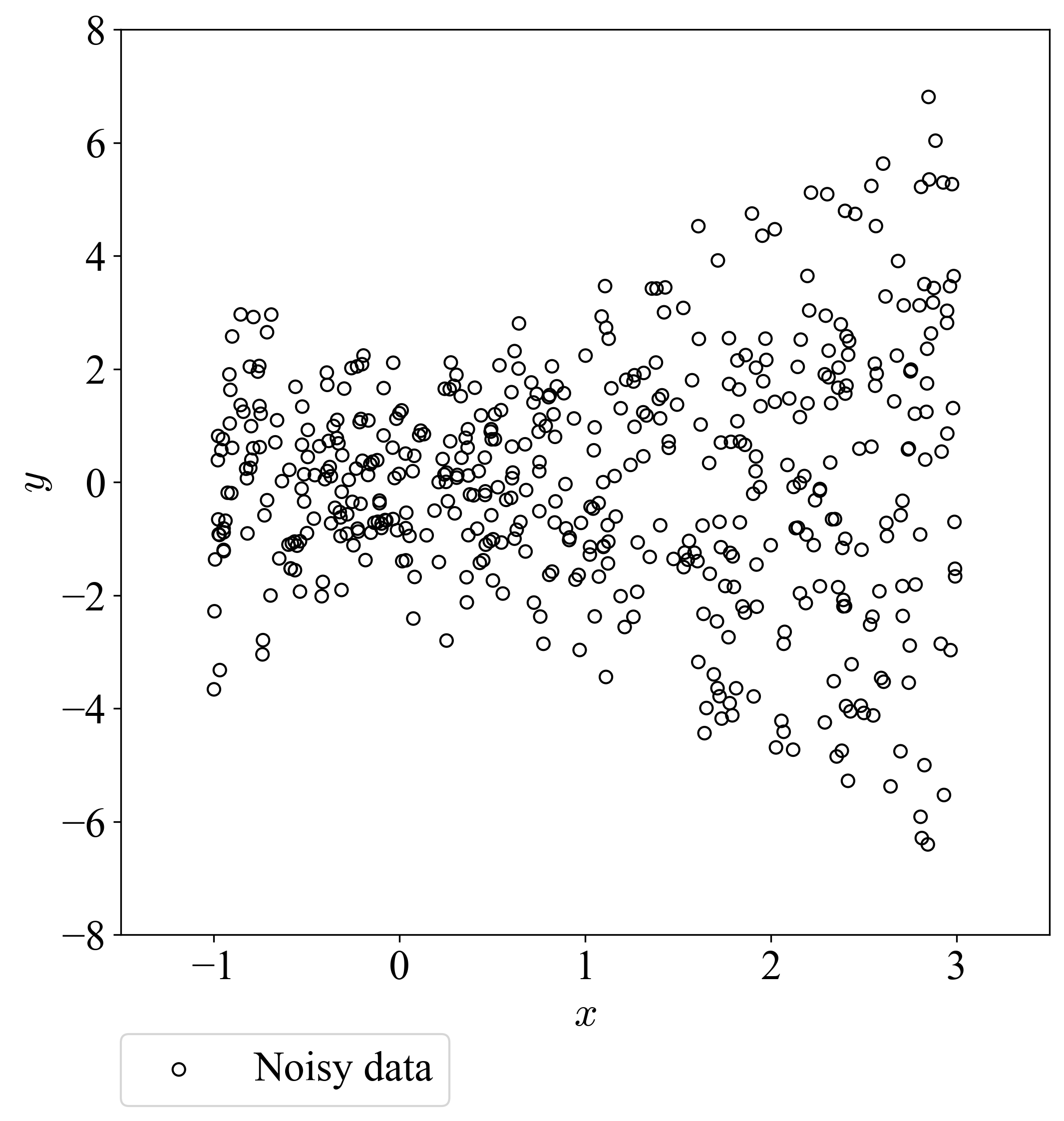
(a) Simulated dataset

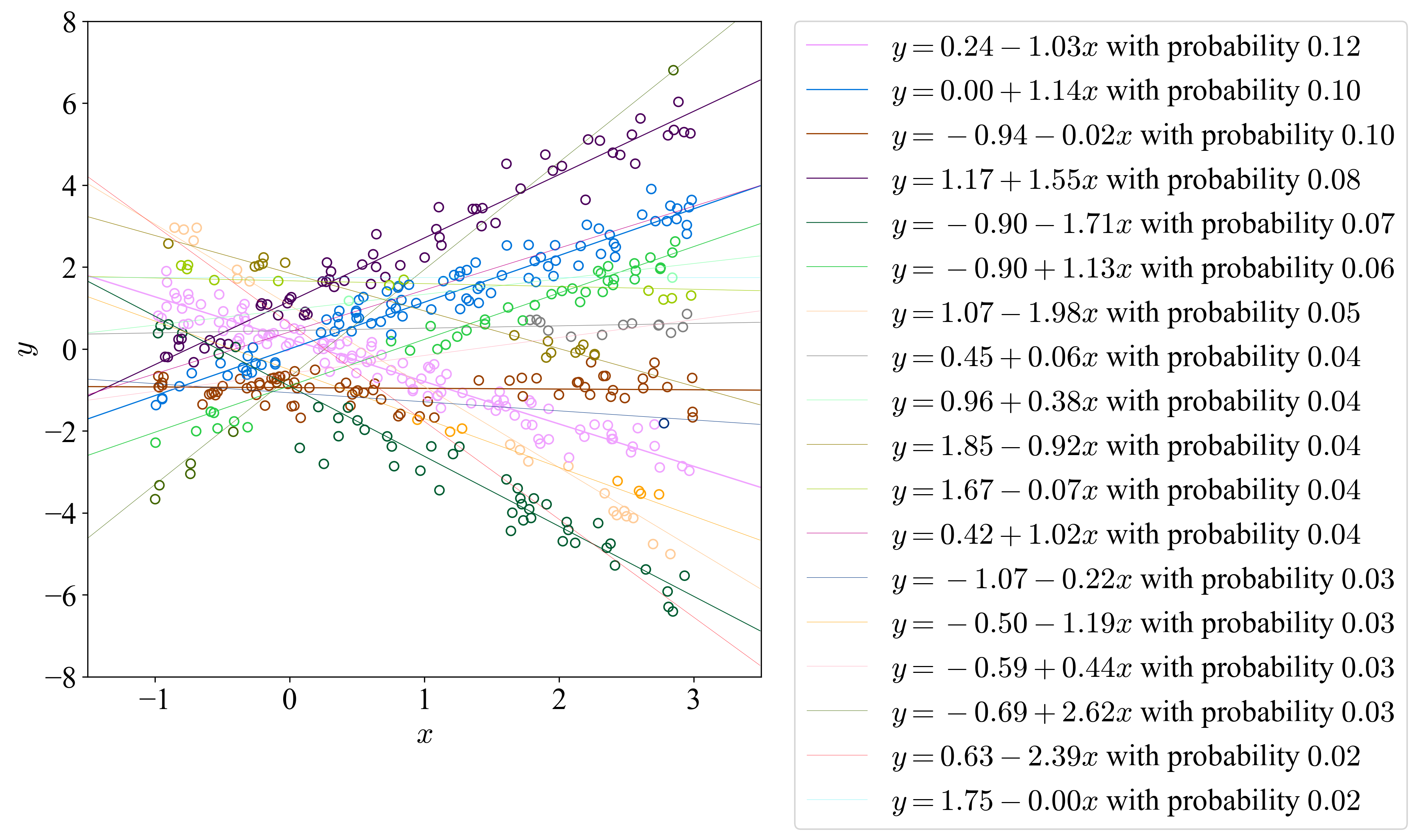
(b) Fitted mixture

Figure 4: Simulation results for $G^{*}$ defined in (33): (a) Scatter plots of simulated dataset where $y$ represents noisy response and $x$ represents univariate covariate; (b) Fitted mixture by NPMLE approach with $\hat{\sigma}=0.44$ chosen by cross-validation.

Our cross-validation procedure gave $\hat{\sigma}=0.44$ which we then used to compute $\hat{G}_{\text{CV}}$ (with $K=[-10,10]^{2}$). Figure 5(a) plots $G^{*}$ and $\hat{G}_{\text{CV}}$ together (the size of each dot corresponds to the mixing probability at that point in $\hat{G}_{\text{CV}}$). Figure 4(b) plots the regression components based on the estimated $\hat{G}_{\text{CV}}$, where the color coding follows the same rule as previously done in Figure 2. Since $G^{*}$ is now a continuous distribution, it is not surprising that the estimated $\hat{G}_{\text{CV}}$ contains many atoms. From Figure 5(a), it is clear that most of the dots corresponding to $\hat{G}_{\text{CV}}$ lie near one of the two circles on which $G^{*}$ is supported. It should also be clear that the the NPMLE with $\sigma$ selected by cross-validation is close to the NPMLE with true $\sigma$. Figure 5(b) compares $(x,y)\mapsto f_{x}^{\hat{G}_{\text{CV}},\hat{\sigma}}(y)$ and $(x,y)\mapsto f_{x}^{\hat{G}}(y)$ with the truth $(x,y)\mapsto f_{x}^{G^{*}}(y)$ and these are reasonably close.

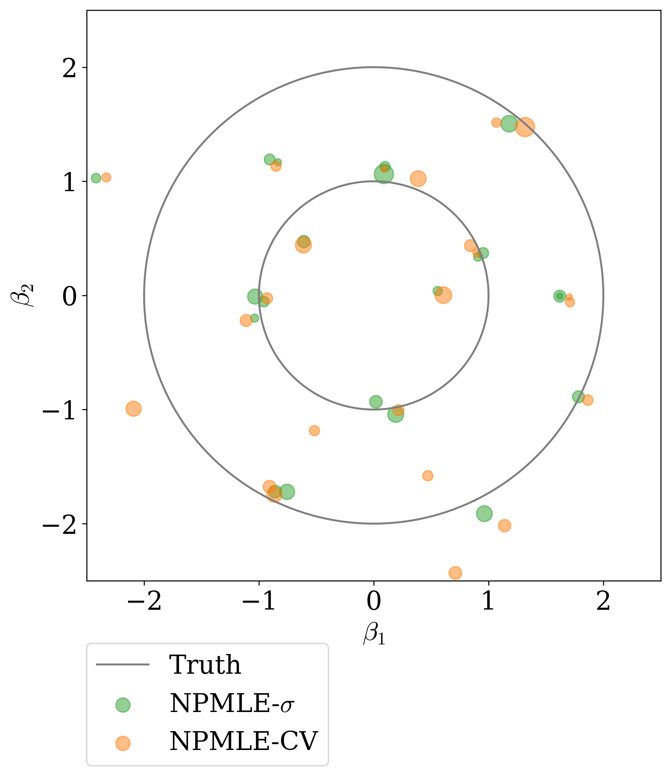
(a) True and fitted measures

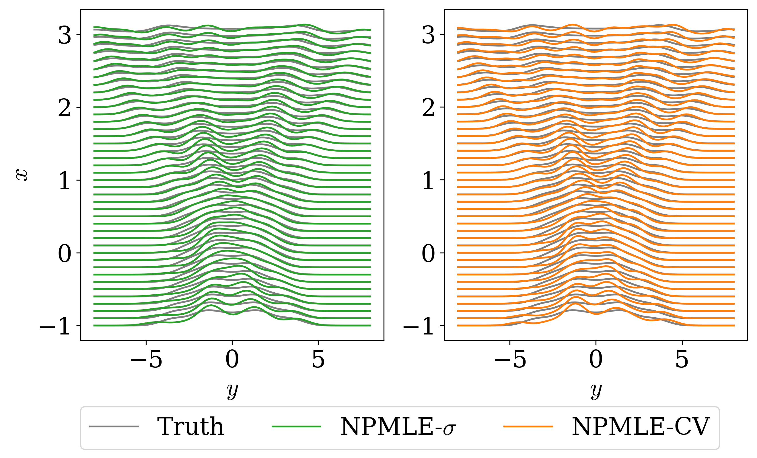
(b) Ridgeline plots

Figure 5: (a) Plots of true $G^{*}$, fitted $\hat{G}$ by NPMLE-$\sigma$ (NPMLE with known $\sigma$), and fitted $\hat{G}_{\text{CV}}$ by NPMLE-CV (NPMLE with $\hat{\sigma}$ selected by cross-validation); (b) Ridgeline plots of density functions $f_{x}^{G^{*}}(y)$ in comparison with its estimates via (i) NPMLE-$\sigma$ (NPMLE with known $\sigma$) and (ii) NPMLE-CV (NPMLE with $\hat{\sigma}$ selected by cross-validation) respectively.

As explained in Section 1, our approach produces an estimate for $\beta^{i}$ for each $i=1,\dots,n$. This estimate is denoted by $\hat{\beta}^{i}_{\mathrm{EB}}$ (defined in (7)) which should be viewed as an approximation to $\hat{\beta}^{i}_{\mathrm{OB}}$ (defined in (5)). In Figure 6, we compare $\hat{\beta}^{i}_{\mathrm{EB}}$ and $\hat{\beta}^{i}_{\mathrm{OB}}$ for $i=1,\dots,n$ by plotting their two coordinates (intercept and slope) separately. That the approximation is working fairly well can easily be seen from the figure.

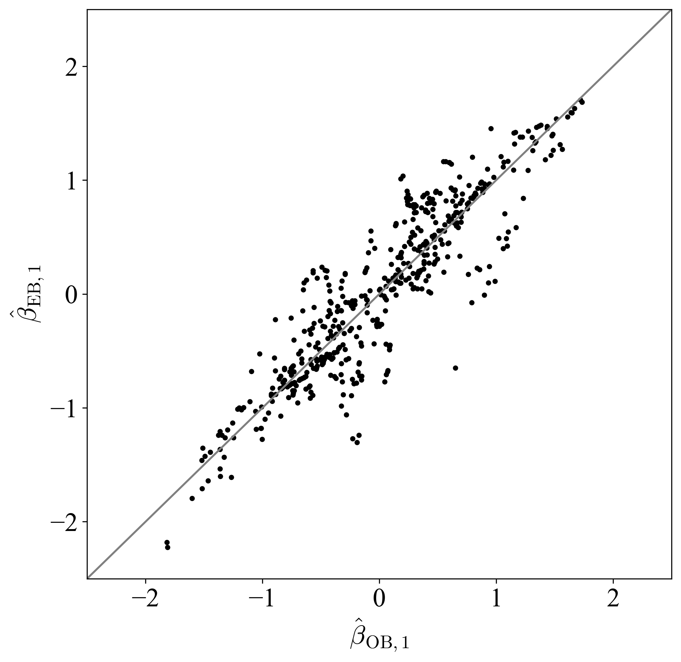
(a) Intercept

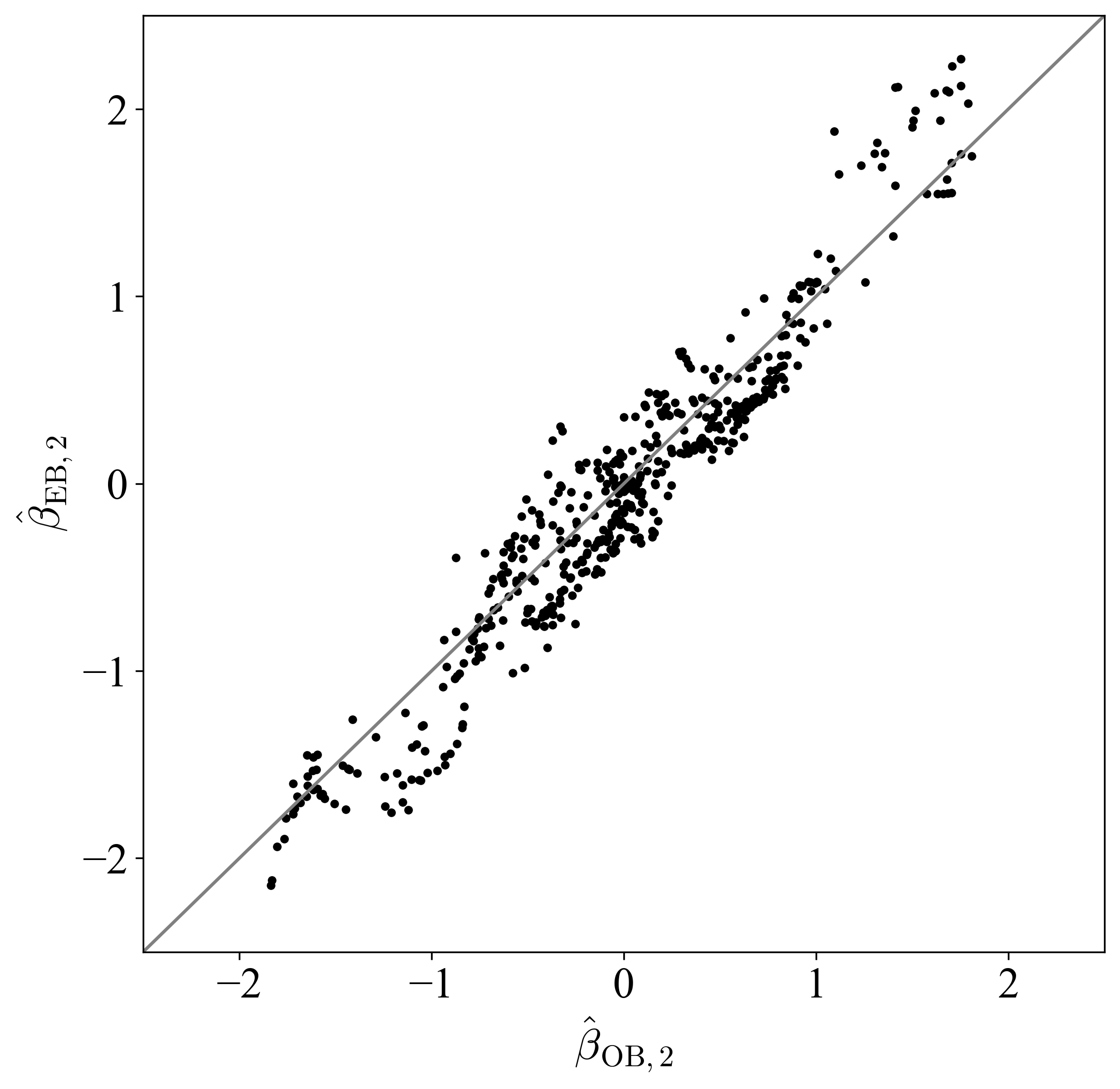
(b) Slope

Figure 6: Plots of $\hat{\beta}_{\mathrm{EB}}^{i}$ against $\hat{\beta}_{\mathrm{OB}}^{i}$ for all $i=1,2,\dots,n$ (when $G^{*}$ is (33)). (a) and (b) show the first (intercept) and the second (slope) component of $\hat{\beta}_{\mathrm{EB}}^{i}$, $\hat{\beta}_{\mathrm{OB}}^{i}$ respectively.

4.4 Simulation Three: Discrete $G^{*}$ with Heteroscedasticity

We now consider data simulated from a finite mixture of regressions model where the variances vary among the components. More specifically, we consider the regression model where the conditional distribution of $Y$ given $X=x$ is

$$Y|X=x\sim\sum_{l}\pi_{l}N(\beta_{l0}+x^{\top}\beta_{l1},\sigma_{l}^{2}).$$ (34)

The component variances $\{\sigma^{2}_{l}\}$ are allowed to change with $l$. This model is actually a special case of (1) because it can be written in the form (1) for

$$G^{*}:=\sum_{l}\pi_{l}\left(N(\beta_{l0},\sigma_{l}^{2}-\sigma^{2})\otimes\delta_{\{\beta_{l1}\}}\right)$$ (35)

for any $\sigma\leq\min_{l}\sigma_{l}$. Here $\delta_{\{\beta_{l1}\}}$ is the degenerate probability distribution concentrated on $\beta_{l1}$ and $N(\beta_{l0},\sigma_{l}^{2}-\sigma^{2})\otimes\delta_{\{\beta_{l1}\}}$ denotes the product of the probability measures $N(\beta_{l0},\sigma_{l}^{2}-\sigma^{2})$ and $\delta_{\{\beta_{l1}\}}$. Also if $\sigma_{l}^{2}=\sigma^{2}$ for some $l$, the probability measure $N(\beta_{l0},\sigma_{l}^{2}-\sigma^{2})$ should be interpreted as $\delta_{\{\beta_{l0}\}}$.

As a consequence, our estimation strategy should also work for the heteroscedastic model (34) and we shall demonstrate this with a simulated dataset here. We would like to note however that our theoretical results do not apply to this setting as $G^{*}$ in (35) has unbounded support. We take a setting similar to Figure 1(a) where the covariate is univariate (generated from the uniform distribution on $[-1,3]$). The parameters $\beta_{l0},\beta_{l1}$ are given by the three lines $3-x,1+1.5x,-1+0.5x$ chosen with probabilities $\pi_{l}$ given by $0.3,0.3,0.4$ (this is exactly the same as in Figure 1(a)). The standard deviations $\sigma_{l}$ vary with $l$ (unlike the case in Figure 1(a)) and we take these to be $\sigma_{1}=0.3$, $\sigma_{2}=0.5,\sigma_{3}=0.7$. Data generated from this model is depicted in Figure 7(a).

We applied our estimation strategy to the data in Figure 7(a). Our cross-validation procedure gave $\hat{\sigma}=0.31$, which is very close to the unknown true smallest heteroscedastic error $\sigma_{1}=0.3$. The result of our estimation procedure can be seen from Figure 7. As before (Figure 2), our approach leads to more lines (compared to the truth) but each fitted line is close to one of the three true lines. Also $(x,y)\mapsto f_{x}^{\hat{G}_{\text{CV}},\hat{\sigma}}(y)$ is an accurate estimate $(x,y)\mapsto f_{x}^{G^{*}}(y)$ as depicted in Figure 8. This accuracy is comparable to the accuracy of $(x,y)\mapsto f_{x}^{\hat{G},\min_{l}\sigma_{l}}(y)$ and that of the estimate obtained by using the EM algorithm with three components initialized at their true values.

(a) Simulated dataset

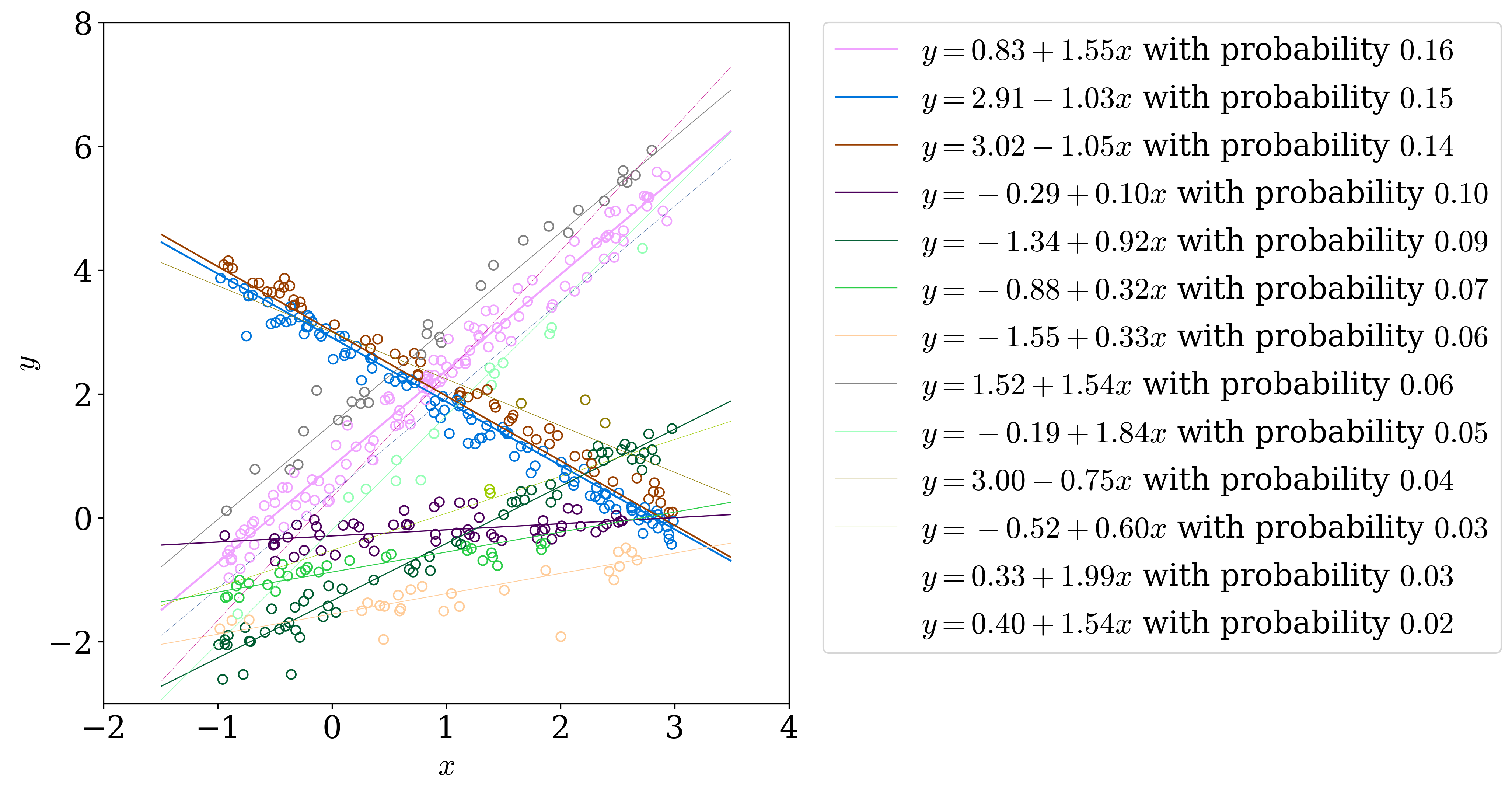
(b) Fitted mixture

Figure 7: Simulation results for $G^{*}=0.3\delta_{\{(3,-1)\}}+0.3\delta_{\{(1,1.5)\}}+0.4\delta_{\{(-1,0.5)\}}$ with heteroscedastic errors $\sigma_{1}=0.3$, $\sigma_{2}=0.5$, $\sigma_{3}=0.7$: (a) Scatter plots of simulated dataset where $y$ represents noisy response and $x$ represents univariate covariate; (b) Fitted mixture by NPMLE approach with $\hat{\sigma}=0.31$ chosen by cross-validation.

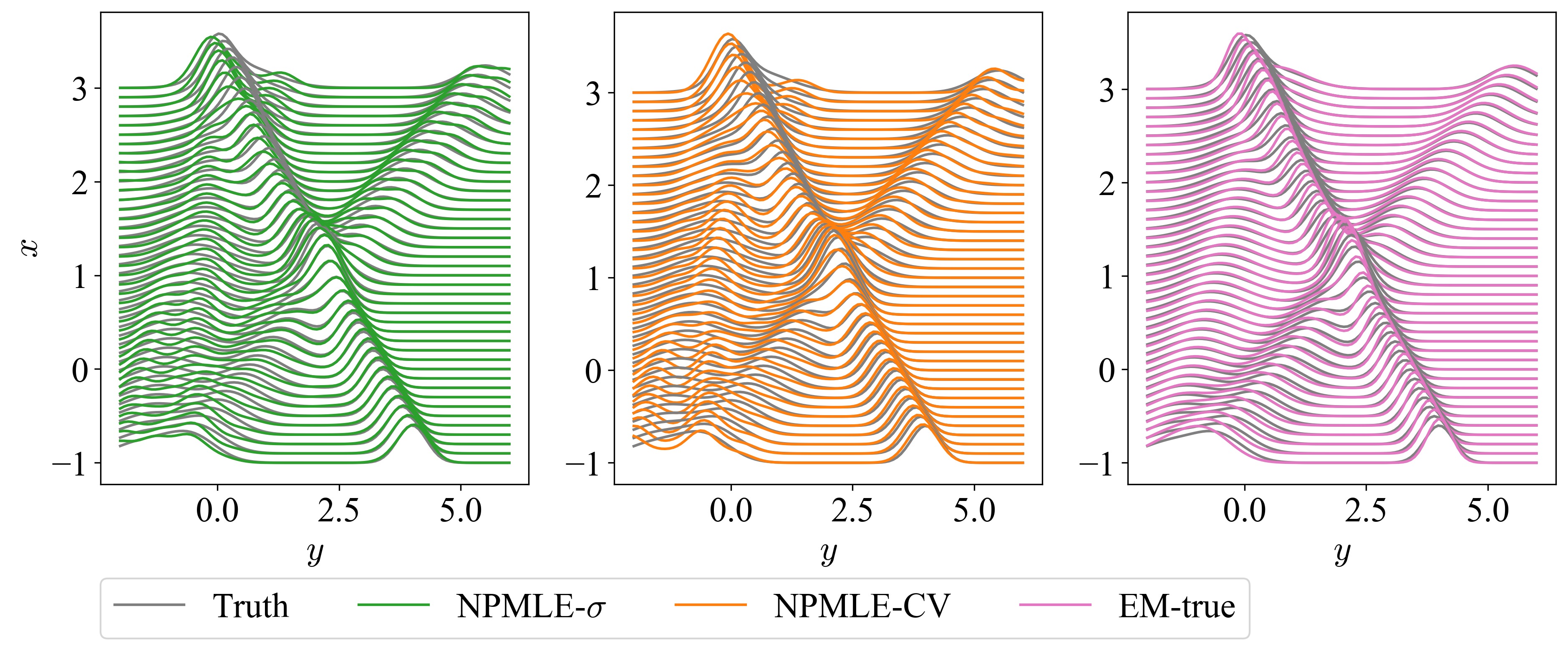
Figure 8: Ridgeline plots of density functions $f_{x}^{G^{*}}(y)$ in comparison with its estimates via (i) NPMLE-$\sigma$ (NPMLE with $\sigma_{1}=\min_{l}\sigma_{l}$, the minimum heteroscedastic error out of $\sigma_{1},\sigma_{2},\sigma_{3}$), (ii) NPMLE-CV (NPMLE with $\hat{\sigma}$ selected by cross-validation), and (iii) EM-true (EM initialized with true parameters of $G^{*}$ and $\sigma$) respectively.

4.5 Real Data Example One: Music Tone Perception

We apply our method to the music tone perception data originally collected by Cohen (1980). This dataset is available, for example, in the R packages mixtools (Benaglia et al., 2009) and fpc (Hennig and Imports, 2015), and has been previously analyzed by De Veaux (1989), Viele and Tong (2002), and Yao and Song (2015). This data was collected in music experiments where a trained musician was presented with a pure fundamental tone plus a series of stretched overtones and was then asked to tune an adjustable tone to the octave above the fundamental tone. The regressor $x$ is the stretching ratio of the overtone to the fundamental tone. The response variable $y$ is the ratio of the adjusted tone to the fundamental by the musician.

At that time of Cohen (1980), there existed two conflicting music perception theories regarding the relationship between $y$ and $x$. One theory states that the adjusted tone is constantly at ratio $2:1$ to the fundamental tone ($y=2$), while the other theory states that the adjusted tone will be equal to the overtone ($y=x$).

While existing studies are built on two-component mixture models with heteroscedastic errors, we apply our NPMLE approach without prior knowledge on number of components. Compared to $500$ data points in simulation settings, there are only $150$ data points in this real dataset, and thus we increase the number of folds in cross-validation correspondingly. We run $10$-fold cross-valition, and the choice of $\sigma$ by cross-validation is $0.05$.

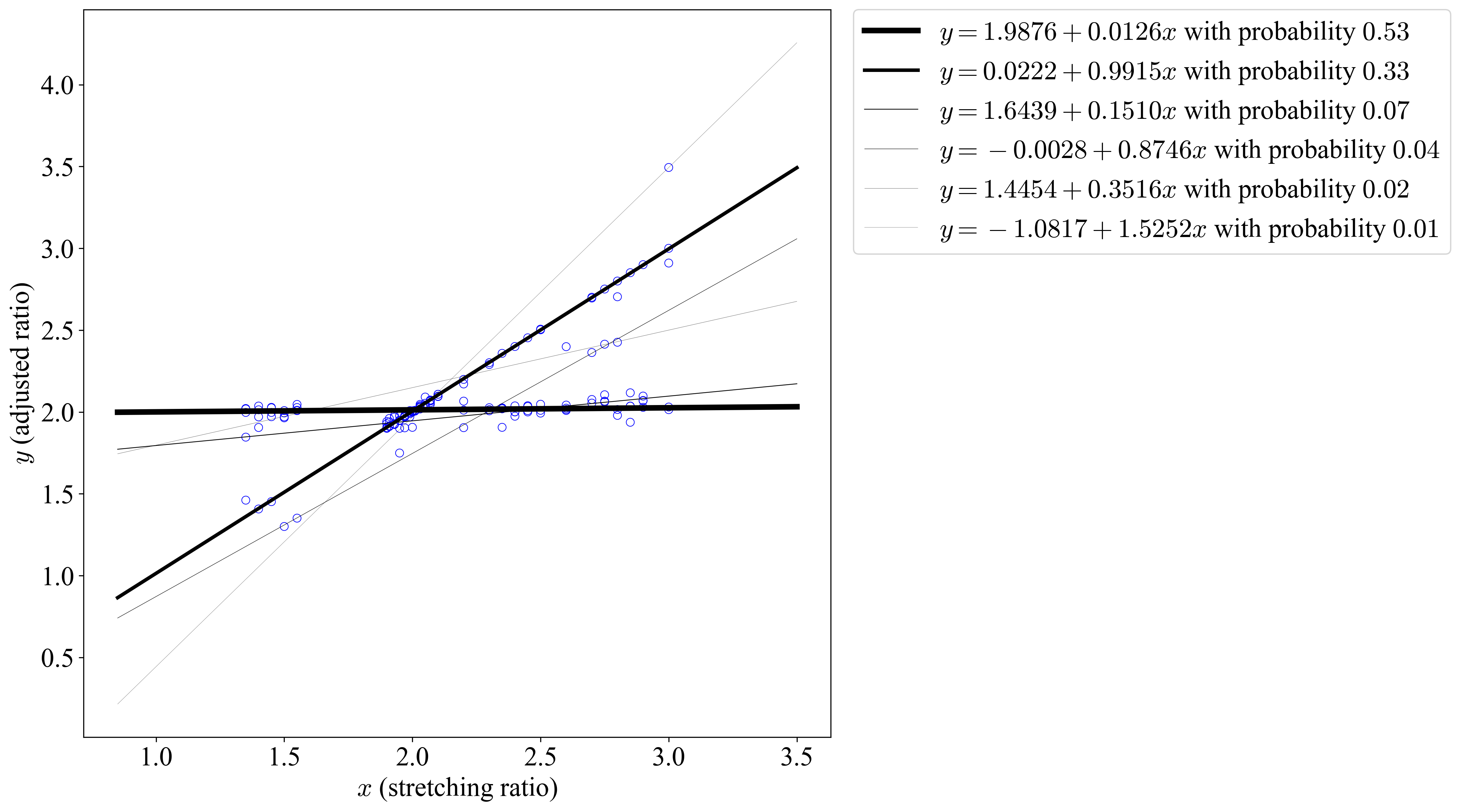
Figure 9: Fitted result of music perception data.

Figure 9 shows the fitted result together with original data points. Similar to our simulation plots, the thickness and darkness of each line in Figure 9 are proportional to the mixing probability of the corresponding component. While there are more than two components in Figure 9, two major components account for most of the mixing probabilities, and all other components occupy very low probabilities. Compared to the two-component modeling in Viele and Tong (2002), the fitted result in Figure 9 attains a considerably higher log-likelihood of 175.50 whereas the highest log-likelihood in Viele and Tong (2002) is 145.52 (our choices of $\sigma$ are rather close). We would like to mention again that the NPMLE approach does not use the prior knowledge of two music theories. Yet, the algorithm is able to identify two major components, which are very close to the conjectural regression functions $y=2$ and $y=x$ respectively.

4.6 Real Data Example Two: CO₂-GDP

Although it seems reasonable to assume a two-component structure in the aforementioned music dataset given the side information of two music perception theories, many real datasets do not come with such a clear structure, and the number of components is unknown. In this example, we apply our NPMLE approach to a real dataset in this latter category.

CO₂ is a greenhouse gas primarily produced from fossil fuel consumption. Increased CO₂ emissions are generally considered to be responsible for global warming. GDP is a measure that reflects a country’s economic wellbeing. Human activities that lead to high GDP often correspond with high CO₂ emissions. Considering both the economy and the environment, it is desirable for countries to achieve high GDP per capita while maintaining low CO₂ per capita. Therefore, the correlation of CO₂ and GDP attracts considerable attention. We retrieve per capita data of 159 countries in year 2015 from Roser (2021). We set the CO₂ emissions per capita (in 10 tons) as the response variable $y$, and set the GDP per capita (in 10,000 USD) as the regressor $x$. A $\sigma$ value of $0.3$ is selected by $10$-fold cross-validation. Previously, the CO₂-GDP relationship has been modeled with mixture of linear regression models with a pre-specified number of components in Hurn et al. (2003) and Huang and Yao (2012).

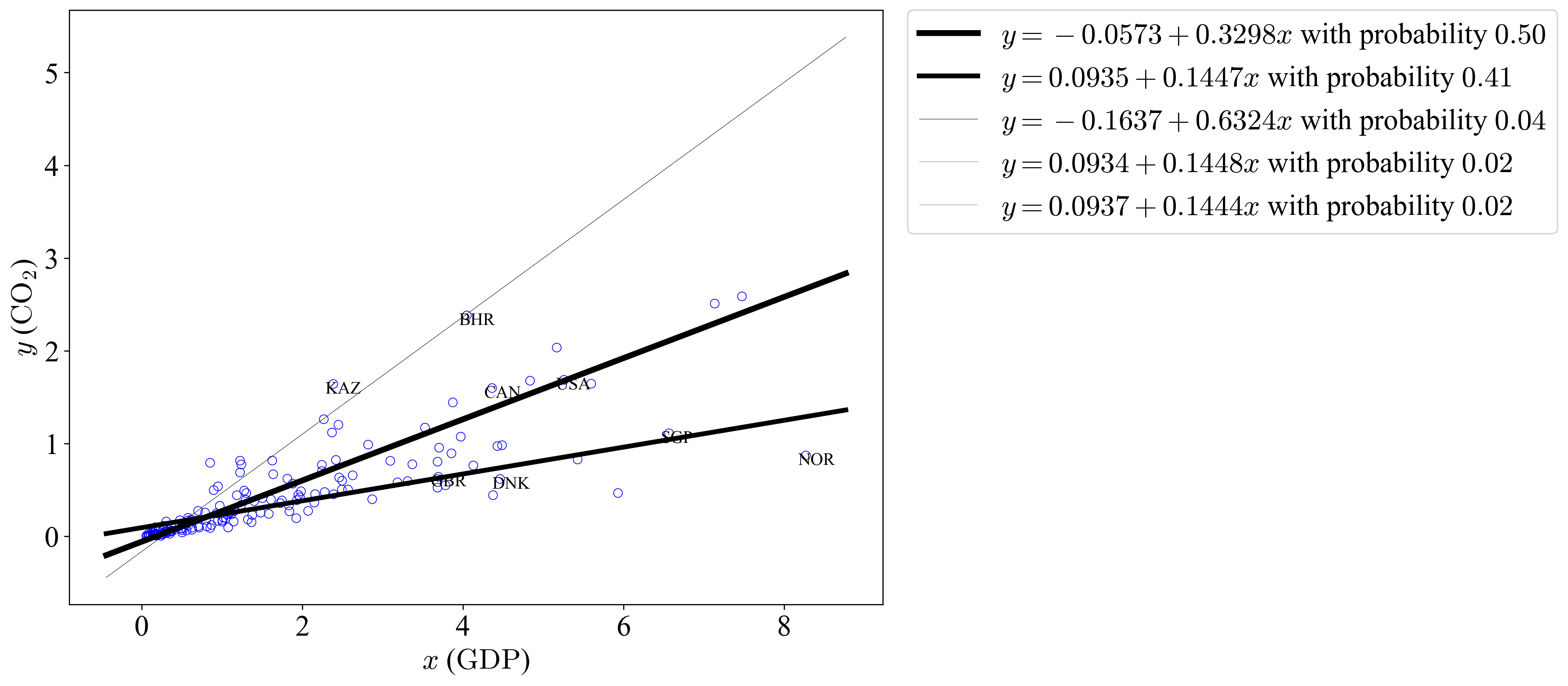
Figure 10: Fitted result of CO₂-GDP data.

Figure 10 shows the fitted result together with original data points. For certain countries, the country’s circle marker in Figure 10 is annotated with its three-digit country code. The thickness and darkness of each line in Figure 10 are proportional to the mixing probability of the corresponding linear regression component. In Figure 10, there are several fitted linear regression components, but only two of them take most of the mixing probabilities. We now take a closer took at these linear regression components in Figure 10. All five components share similar intercepts, which are all close to $0$, but the slopes differ. The component with the highest mixing probability has a medium slope value, and countries near this component include Canada, United States, etc. The component with the highest slope value has a very low mixing probability, and countries near this component include Bahrain, Kazakhstan, etc. The component with the lowest slope value has a relative high mixing probability, and countries near this component include Great Britain, Denmark, Norway, etc. Interestingly, countries in the same component seem to be geographically close, or similarly rich in fossil fuel resources. The fitted result indicates the 159 countries can be effectively categorized to several groups in terms of CO₂ emissions and GDP growth relationship. The identification of such subgroups can help to illustrate potential developing paths of lower GDP countries, which was pointed out in Hurn et al. (2003).

5 Extension to Mixture of Nonlinear Regression

In this section, we argue that the NPMLE approach can also be applied to the more general case of mixtures of nonlinear regression models. Here the conditional distribution of $Y$ given $X=x$ is given by the density

$$y\mapsto f_{x}^{G^{*}}(y):=\int\frac{1}{\sigma}\phi\left(\frac{y-r(x,\beta)}{\sigma}\right)dG^{*}(\beta)$$ (36)

where $r(x,\beta)$ represents a possibly nonlinear regression function parametrized by a $\mathfrak{p}$-dimensional parameter $\beta$. The covariate $x$, as before, has dimension $p$. The dimensions $\mathfrak{p}$ (of $\beta$) and $p$ (of $x$) are not necessarily equal.

Our estimation strategy can be extended to the problem of estimating $G^{*}$ from $n$ independent observations $(x_{1},y_{1}),\dots,(x_{n},y_{n})$ drawn from the above model. Assuming that $G^{*}$ is supported on $\mathrm{B}_{\mathfrak{p}}(0,R):=\{\beta\in\mathbb{R}^{\mathfrak{p}}:\|\beta\|\leq R\}$ for a known constant $R>0$, we estimate $G^{*}$ by the NPMLE defined via

$$\hat{G}\in\underset{G\text{ supported on }K}{\mathrm{argmax}}\sum_{i=1}^{n}\log\left[\frac{1}{\sigma}\int\phi\left(\frac{y_{i}-r(x_{i},\beta)}{\sigma}\right)dG(\beta)\right].$$ (37)

The existence of $\hat{G}$ in (37) when $K$ is compact follows from the same argument as in the proof of Theorem 1. Our computational algorithm from Subsection 2.2 based on the CGM can be used with little modification (basically $x_{i}^{\top}\beta$ must now be replaced by $r(x_{i},\beta)$) to compute the above estimator $\hat{G}$. We initialize the CGM with $\mathrm{f}^{(0)}=\mathrm{f}^{\beta}$ where $\beta$ is a random point in $K$. The cross validation procedure to choose $\sigma$ also works analogously as before.

We have found that our estimation strategy works well for estimation under the model (36) for several different nonlinear functions $r(\cdot,\cdot)$ including polynomials, exponentials and trigonometric functions. As illustration, consider the data shown in Figure 11(a). These are 500 points generated independently from the model (36) with

$$r(x,\beta):=\beta_{1}+\sin(\beta_{2}x).$$

The probability measure $G^{*}$ is given by $0.5\delta_{\{\beta_{1}=-0.5,\beta_{2}=1\}}+0.5\delta_{\{\beta_{1}=-1.5,\beta_{2}=1.5\}}$ and $\sigma$ is given by $\sigma=0.5$.

$$G^{*}:=0.5\delta_{\{\beta_{1}=-0.5,\beta_{2}=1\}}+0.5\delta_{\{\beta_{1}=-1.5,\beta_{2}=1.5\}}.$$

In other words, the true regression function equals one of the two nonlinear functions $x\mapsto-0.5+\sin x$ and $x\mapsto-1.5+\sin(1.5x)$ with equal probability. These two functions are also plotted in Figure 11(a) and the individual data points are colored according to the function which generated them. These colors (and the curves corresponding to the true functions) are of course not available to the data analyst. While applying our method to this dataset, we make the assumption that the component regression functions are known to be of the form $x\mapsto\beta_{1}+\sin(\beta_{2}x)$ but we do not know the values of $(\beta_{1},\beta_{2})$.

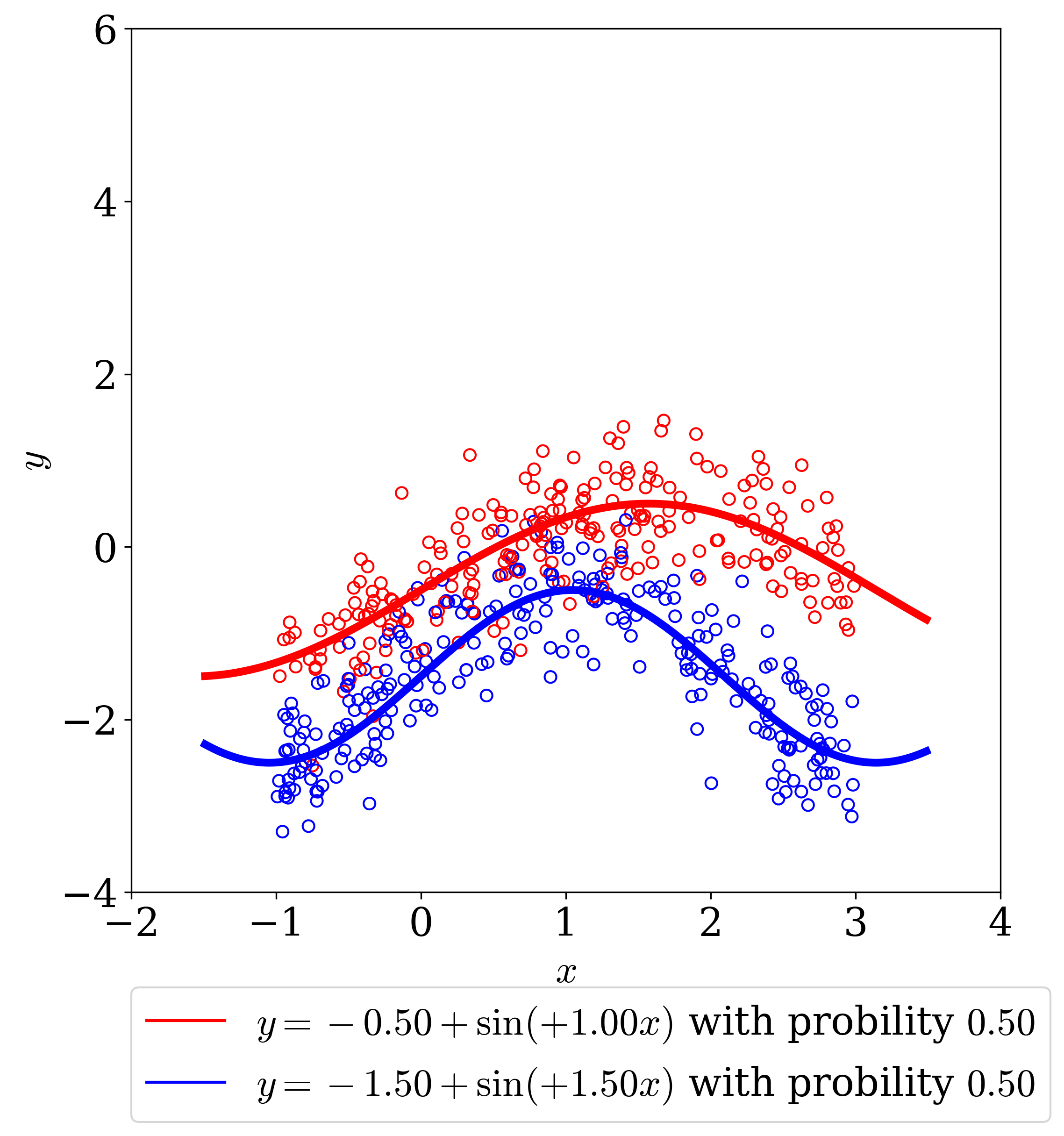
(a) True mixture

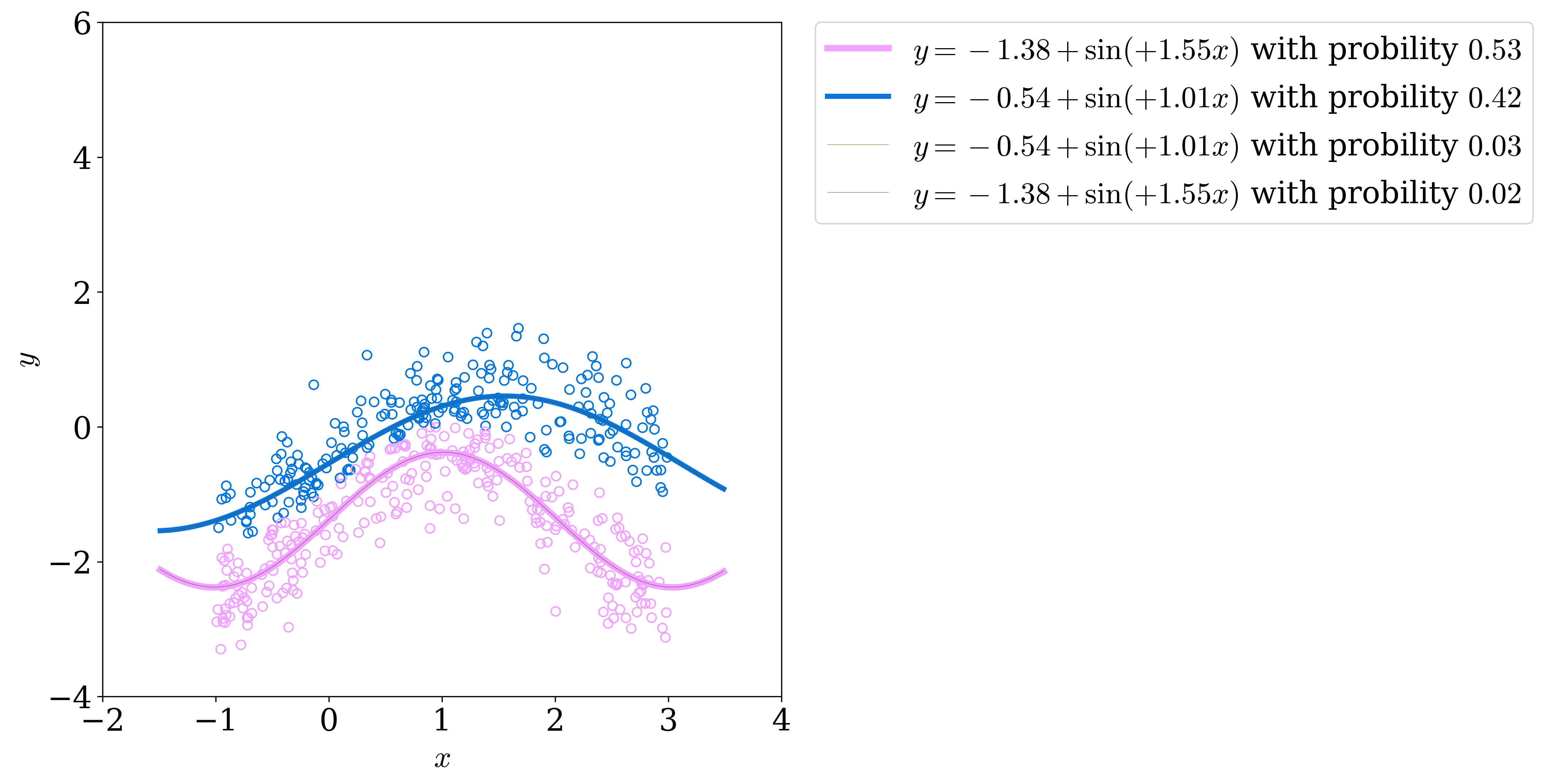
(b) Fitted mixture by NPMLE-CV

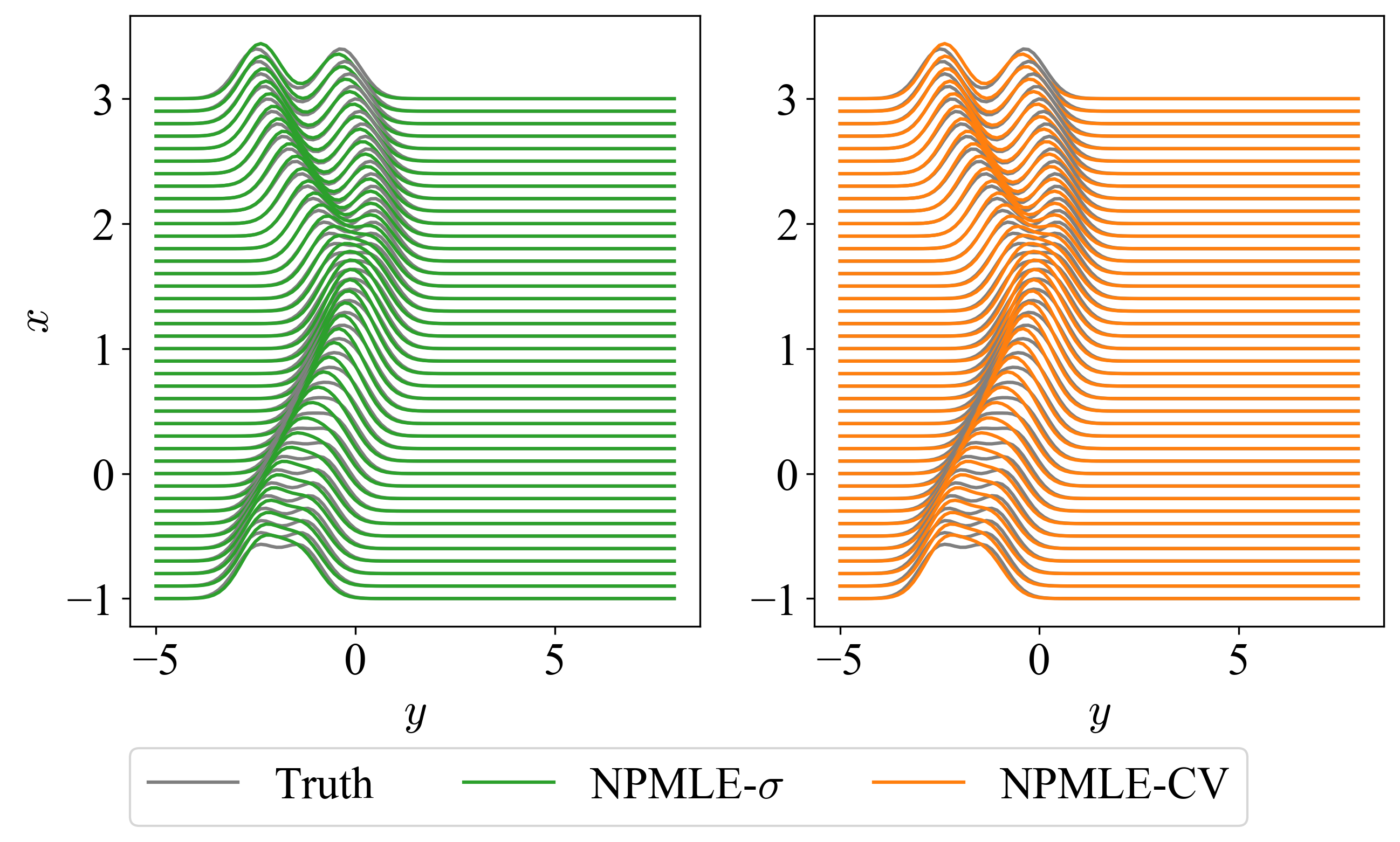
(c) Ridgeline plots of density functions

Figure 11: Data and results for the mixture of trigonometric regression model: (a) True mixture; (b) Fitted mixture by NPMLE-CV with the chosen scale parameter $\hat{\sigma}=0.46$ by cross-validation; Some estimated regression equations appear to be repeated because these equations are very close to each other and we have rounded the estimates for plotting purposes. (c) Ridgeline plots of density functions $f_{x}^{G^{*}}(y)$ in comparison with its estimates via (i) NPMLE-$\sigma$ (NPMLE with known $\sigma$) and (ii) NPMLE-CV (NPMLE with $\hat{\sigma}$ selected by cross-validation) respectively.

The results of applying our method to the data in Figure 11(a) are shown in Figures 11(b) and 11. We took $K$ in (37) to be $K=[-10,10]^{2}$. $\sigma$ was estimated by $\hat{\sigma}=0.46$ and the fitted $\hat{G}$ had four components. Our method estimated 4 regression components but two of them are very close (up to rounding errors) to $-1.38+\sin(1.55x)$ and the other two are very close to $-0.54+\sin(1.01x)$. These are, in turn, quite closely aligned with the true regression functions $x\mapsto-1.5+\sin(1.5x)$ and $x\mapsto-0.5+\sin x$. The estimated probabilities of these two components were $0.55$ and $0.45$ respectively (while the true probabilities were equal to $0.5$). Figure 11 shows that the estimated density function

$$(x,y)\mapsto\int\frac{1}{\hat{\sigma}}\phi\left(\frac{y-r(x,\beta)}{\hat{\sigma}}\right)d\hat{G}_{\textrm{cv}}(\beta)$$

is an accurate estimator for

$$(x,y)\mapsto\int\frac{1}{\sigma}\phi\left(\frac{y-r(x,\beta)}{{\sigma}}\right)d{G^{*}}(\beta)$$

and the accuracy is compared to that of our estimator computed with $\sigma$ known to be its true value.

It would be of interest to extend the theoretical results of Section 3. We do not know how to do this for a large class of nonlinear functions $r(\cdot,\cdot)$. Let us just remark here that it is straightforward to extend Theorem 28 to the case where $r(x,\beta)$ is a polynomial in $\beta$. This leads to the following theorem.

Theorem 6.

Consider data $(x_{1},y_{1}),\dots,(x_{n},y_{n})$ with $n\geq 3$ where $x_{1},\dots,x_{n}$ are fixed design points and $y_{1},\dots,y_{n}$ are independent with $y_{i}$ having the density (36) with $x=x_{i}$. Assume that, for every $x$, the function $\beta\mapsto r(x,\beta)$ is a polynomial of degree at most $\zeta$. Assume that $G^{*}\left\{\beta\in\mathbb{R}^{\mathfrak{p}}:\|\beta\|\leq R\right\}=1$ for some $R>0$ and that $\mathfrak{L}$ is a positive quantity such that

$$\sup_{\beta_{1},\beta_{2}\in B_{\mathfrak{p}}(0,R):\beta_{1}\neq\beta_{2}}\frac{\left|r(x_{i},\beta_{1})-r(x_{i},\beta_{2})\right|}{\|\beta_{1}-\beta_{2}\|}\leq\mathfrak{L}\qquad\text{for all $i=1,\dots,n$}.$$ (38)

Then inequalities (27) and (28) hold with $\epsilon_{n}^{2}$ replaced by

$$\epsilon^{2}_{n}=n^{-1}\left(\zeta^{\mathfrak{p}}\left(\mathrm{Log}~{}\frac{n}{\sqrt{\sigma}\zeta^{\mathfrak{p}}}\right)^{\mathfrak{p}+1},\left(\frac{\zeta R\mathfrak{L}}{\sigma}\right)^{\mathfrak{p}}\left(\mathrm{Log}~{}\left\{\frac{n}{\sqrt{\sigma}}\left(\frac{\sigma}{\zeta R\mathfrak{L}}\right)^{\mathfrak{p}}\right\}\right)^{\frac{\mathfrak{p}}{2}+1}\right).$$ (39)

The rate given in (39) has the same qualitative behavior as the rates of Theorem 28 and Theorem 4. Specifically it is $O(n^{-1}(\log n)^{p+1})$ assuming that $\zeta,R,\mathfrak{L}$ are all fixed. Theorem 28 can be viewed as a special case of Theorem 39 with $\mathfrak{p}=p$, $r(x,\beta)=x^{\top}\beta$, and $\zeta=1$. Also $\mathfrak{L}$ (defined in (38)) can be taken as any value that is at least $\max_{1\leq i\leq n}\|x_{i}\|$ because, by the Cauchy-Schwarz inequality,

$$|r(x_{i},\beta_{1})-r(x_{i},\beta_{2})|=|x_{i}^{\top}(\beta_{1}-\beta_{2})|\leq\|x_{i}\|\|\beta_{1}-\beta_{2}\|\qquad\text{ for $i=1,\dots,n$.}$$

Under the assumption $\max_{1\leq i\leq n}\|x_{i}\|\leq B$ in Theorem 28, one can thus take $\mathfrak{L}=B$ in (39) and this yields the conclusion of Theorem 28.

6 Proofs

6.1 Proof of Theorem 1

The notation for $\mathrm{f}^{G}$, $\mathrm{f}^{\beta}$ and $\mathcal{P}_{K}$ introduced at the beginning of Subsection 2.1 will be used in the proof below.

Proof of Theorem 1.

The objective function in the optimization problem (12) only depends on $G$ through the vector $\mathrm{f}^{G}$. As a result, (12) is equivalent to

$$\mathop{\rm argmax}\left\{\frac{1}{n}\sum_{i=1}^{n}\log\mathrm{f}(i):\mathrm{f}\in\mathcal{Q}_{K}\right\}$$ (40)

where $\mathrm{f}(i)$ denotes the $i^{th}$ element of the vector $\mathrm{f}\in\mathbb{R}^{n}$ and

$$\mathcal{Q}_{K}=\{\mathrm{f}^{G}\,:\,G\text{ is any probability measure supported on }K\}.$$

The set $\mathcal{Q}_{K}$ need not be compact in general. We claim that

$$\mathcal{Q}_{K}\subseteq\mathrm{conv}(\mathrm{cl}(\mathcal{P}_{K}))$$ (41)

where $\mathrm{cl}$ denotes closure and $\mathrm{conv}$ denotes convex hull. This claim will be proved later. The set $\mathrm{conv}(\mathrm{cl}(\mathcal{P}_{K}))$ is compact because $\mathrm{cl}(\mathcal{P}_{K})$ is compact (as $\mathcal{P}_{K}\subseteq[0,1/(\sqrt{2\pi}\sigma)]^{n}$ is bounded) and as the convex hull of a compact set in Euclidean space is compact (see, for example, (Bertsekas et al., 2003, Proposition 1.3.2)). Therefore a solution $\hat{\mathrm{f}}\in\mathrm{conv}(\mathrm{cl}(\mathcal{P}_{K}))$ exists for the optimization problem

$$\mathop{\rm argmax}\left\{\frac{1}{n}\sum_{i=1}^{n}\log\mathrm{f}(i):\mathrm{f}\in\mathrm{conv}(\mathrm{cl}(\mathcal{P}_{K}))\right\}.$$ (42)

Further the solution $\hat{\mathrm{f}}$ is unique as the objective function $L(\mathrm{f}):=\frac{1}{n}\sum_{i=1}^{n}\log\mathrm{f}(i)$ is strictly concave. Moreover $\hat{\mathrm{f}}$ lies in the boundary of the set $\mathrm{conv}(\mathrm{cl}(\mathcal{P}_{K}))$ because otherwise $\nabla L(\hat{\mathrm{f}})^{\top}=({1}/{\hat{\mathrm{f}}(1)},\dots,{1}/{\hat{\mathrm{f}}(n)})$ would have to be zero which is impossible. As a result, by the the Carathéodory theorem (see, for example, (Silvey, 1980, Appendix 2)), $\hat{\mathrm{f}}$ can be written as a convex combination of at most $n$ points in $\mathrm{cl}(\mathcal{P}_{K})$ i.e., $\hat{\mathrm{f}}=\sum_{j=1}^{N}\pi_{j}g_{j}$ for some $N\leq n$, $g_{j}\in\mathrm{cl}(\mathcal{P}_{K})$ and $\pi_{j}>0$ with $\sum_{j}\pi_{j}=1$. We now claim that under the assumptions on $K$ given in the statement of Theorem 1, for every $g\in\mathrm{cl}(\mathcal{P}_{K})$, there exists $\beta\in K$ such that

$$g(i)I\{g(i)>0\}=\mathrm{f}^{\beta}(i)I\{g(i)>0\}.$$ (43)

Assuming the validity of this claim (which will be proved later), there exists $\beta_{j}\in K$ for which

$$g_{j}(i)I\{g_{j}(i)>0\}=\mathrm{f}^{\beta_{j}}(i)I\{g_{j}(i)>0\}\qquad\text{for $j=1,\dots,N$}.$$ (44)

Now if $g_{j}(i)=0$ for some $j$ and $i$, we would have $\sum_{j}\pi_{j}\mathrm{f}^{\beta_{j}}$ having a higher objective value compared to $\hat{\mathrm{f}}=\sum_{j}\pi_{j}\mathrm{f}^{\beta_{j}}$ (note that all components of $\mathrm{f}^{\beta}$ are all strictly positive for every $\beta$) which would contradict the fact that $\hat{\mathrm{f}}$ is the unique solution to (42). We thus have $g_{j}(i)>0$ for all $i$ which implies, by (44), that $g_{j}=\mathrm{f}^{\beta_{j}}$ for every $j$. This obviously implies that $g_{j}\in\mathcal{P}_{K}$ so that $\hat{\mathrm{f}}\in\mathrm{conv}(\mathcal{P}_{K})$. Also

$$\hat{\mathrm{f}}=\sum_{j=1}^{N}\pi_{j}\mathrm{f}^{\beta_{j}}=\mathrm{f}^{\hat{G}}\in\mathrm{conv}(\mathcal{P}_{K})\qquad\text{where $\hat{G}=\sum_{i=1}^{N}\pi_{j}\delta_{\{\beta_{j}\}}$}.$$

As a result $\hat{\mathrm{f}}\in\mathcal{Q}_{K}$ which shows that $\hat{\mathrm{f}}$ is the unique solution to (40) and this completes the proof of Theorem 1. We only need to prove the two claims (41) and (43).

For (41), take $\mathrm{f}^{G}\in\mathcal{Q}_{K}$ where $G$ is a probability measure on $K$. By Parthasarathy (2005, Theorem 6.3), there exist discrete probability measures $\{\mu_{m}\}_{m=1}^{\infty}$ with finite supports converging weakly to $G$ as $m\rightarrow\infty$ and this implies $f^{\mu_{m}}_{x_{i}}(y_{i})\rightarrow f^{G}_{x_{i}}(y_{i})$ for $i=1,\dots,n$. As a result, $\mathrm{f}^{\mu_{m}}\rightarrow\mathrm{f}^{G}$ as $m\rightarrow\infty$. This implies that

$$\mathcal{Q}_{K}\subseteq\mathrm{cl}(\mathrm{conv}(\mathcal{P}_{K})).$$

because each $\mathrm{f}^{\mu_{m}}\in\mathrm{conv}(\mathcal{P}_{K})$. To complete the proof of (41), it is enough to show that

$$\mathrm{conv}(\mathrm{cl}(\mathcal{P}_{K}))=\mathrm{cl}(\mathrm{conv}(\mathcal{P}_{K})).$$ (45)

For (45), first note that $\mathcal{P}_{K}\subseteq\mathrm{conv}(\mathcal{P}_{K})$ which implies $\mathrm{cl}(\mathcal{P}_{K})\subseteq\mathrm{cl}(\mathrm{conv}(\mathcal{P}_{K}))$. $\mathrm{cl}(\mathrm{conv}(\mathcal{P}_{K}))$ is convex, and $\mathrm{conv}(\mathrm{cl}(\mathcal{P}_{K}))$ is the smallest convex set that contains $\mathrm{cl}(\mathcal{P}_{K})$, so

$$\mathrm{conv}(\mathrm{cl}(\mathcal{P}_{K}))\subseteq\mathrm{cl}(\mathrm{conv}(\mathcal{P}_{K})).$$

For the other inclusion, observe that, as noted earlier, $\mathrm{conv}(\mathrm{cl}(\mathcal{P}_{K}))$ is compact so that

$$\mathrm{conv}(\mathrm{cl}(\mathcal{P}_{K}))=\mathrm{cl}(\mathrm{conv}(\mathrm{cl}(\mathcal{P}_{K})))\supseteq\mathrm{cl}(\mathrm{conv}((\mathcal{P}_{K}))).$$

This proves (45) and consequently (41).

We next prove (43). Fix $g\in\mathrm{cl}(\mathcal{P}_{K})$. If $K$ is compact, then $\mathcal{P}_{K}$ is also compact so that $g\in\mathcal{P}_{K}$ which means that $g=\mathrm{f}^{\beta}$ for some $\beta\in K$ and this proves (43). So let us assume that $K$ is not necessarily compact and that the second assumption in the statement of Theorem 1 holds.

Let $I:=\{1\leq i\leq n:\mathrm{g}(i)>0\}$ and let $V$ be the linear subspace of $\mathbb{R}^{p}$ spanned by $\{x_{i}|i\in I\}$ (recall that $x_{1},\dots,x_{n}$ are the observed covariate vectors). Because $g\in\mathrm{cl}(\mathcal{P}_{K})$, we can write $g=\lim_{l\rightarrow\infty}\mathrm{f}^{\beta_{l}}$ for some sequence $\{\beta_{l}\}$ in $K$. For $l\geq 1$, let $\alpha_{l}$ denote the projection of $\beta_{l}$ onto $V$ so that $x_{i}^{\top}\alpha_{l}=x_{i}^{\top}\beta_{l}$ for all $i\in I$ and all $l\geq 1$. Also by our assumption on $K$, we have $\alpha_{l}\in K$. We will show that $\{\alpha_{l}\}_{l=1}^{\infty}$ is bounded.

For $i\in I$, $\mathrm{g}(i)>0$ thus $\{x_{i}^{\top}\beta_{l}\}_{l=1}^{\infty}$ is bounded and $\lim_{l\rightarrow\infty}x_{i}^{\top}\beta_{l}$ exists. Since $x_{i}^{\top}\alpha_{l}=x_{i}^{\top}\beta_{l}$, $\{x_{i}^{\top}\alpha_{l}\}_{l=1}^{\infty}$ is also bounded. Take an orthonormal basis of $V$ as $r_{1},r_{2},\dots,r_{v}$. For any $j=1,\dots,v$, since $V$ is spanned by $\{x_{i}|i\in I\}$, $r_{j}$ is a linear combination of $\{x_{i}|i\in I\}$. Therefore, as a linear combination of $\{x_{i}^{\top}\alpha_{l}\}_{l=1}^{\infty}$, $\{r_{j}^{\top}\alpha_{l}\}_{l=1}^{\infty}$ is bounded (noting that the linear combination coefficients do not depend on $l$). Because

$$\alpha_{l}^{\top}\alpha_{l}=\sum_{j=1}^{v}(r_{j}^{\top}\alpha_{l})^{2},$$

it follows that $\{\alpha_{l}^{\top}\alpha_{l}\}_{l=1}^{\infty}$ is also bounded. Now we can take a convergent subsequence of $\{\alpha_{l}\}_{l=1}^{\infty}$. The limit of the subsequence, denoted by $\beta$, also belongs to $K$ because $K$ is assumed to be closed. For $i\in I$, $x_{i}^{\top}\beta=\lim_{l\rightarrow\infty}x_{i}^{\top}\beta_{l}$. Let $\mathrm{f}^{\beta}$ denote the atomic likelihood vector with respect to $\beta$, then $\mathrm{f}^{\beta}(i)=\mathrm{g}(i)$ for all $i\in I$. This proves (43) and thereby completes the proof of Theorem 1. ∎

6.2 Proof of Theorem 2

Proof of Theorem 2.

Fix $k\geq 0$. By definition of $\Psi_{k}$ and the fact that $\mathrm{f}^{(k+1)}$ solves (17), we have

$$L(\mathrm{f}^{(k+1)})\geq L\left((1-\gamma_{k})\mathrm{f}^{(k)}+\gamma_{k}\tilde{g}^{(k)}\right)=L(\mathrm{f}^{(k)})+\gamma_{k}\left<\tilde{g}^{(k)}-\mathrm{f}^{(k)},\nabla L(\mathrm{f}^{(k)})\right>-\frac{\gamma_{k}^{2}}{2}\Psi_{k}.$$ (46)

By (20), we have

$$\left<\tilde{g}^{(k)}-\mathrm{f}^{(k)},\nabla L(\mathrm{f}^{(k)})\right> \geq\max_{g\in\mathcal{P}_{K}}\left<g-\mathrm{f}^{(k)},\nabla L(\mathrm{f}^{(k)})\right>-\delta_{k}$$

$$=\max_{g\in\text{conv}(\mathcal{P}_{K})}\left<g-\mathrm{f}^{(k)},\nabla L(\mathrm{f}^{(k)})\right>-\delta_{k}\geq\left<\hat{\mathrm{f}}-\mathrm{f}^{(k)},\nabla L(\mathrm{f}^{(k)})\right>-\delta_{k}.$$ (47)

Using concavity of $L(\cdot)$, we get

$$\left<\hat{\mathrm{f}}-f^{(k)},\nabla L(\mathrm{f}^{(k)})\right>\geq L(\hat{\mathrm{f}})-L(\mathrm{f}^{(k)}).$$ (48)

Combining the above three inequalities, we obtain

$$L(\mathrm{f}^{(k+1)})\geq L(\mathrm{f}^{(k)})+\gamma_{k}\left(L(\hat{\mathrm{f}})-L(\mathrm{f}^{(k)})\right)-\delta_{k}-\frac{\gamma_{k}^{2}}{2}\Psi_{k}$$

which is equivalent to

$$L(\hat{\mathrm{f}})-L(\mathrm{f}^{(k+1)})\leq(1-\gamma_{k})\left(L(\hat{\mathrm{f}})-L(\mathrm{f}^{(k)})\right)+\delta_{k}+\frac{\gamma_{k}^{2}}{2}\Psi_{k}.$$ (49)

We shall prove

$$L(\hat{\mathrm{f}})-L(\mathrm{f}^{(k+1)})\leq\frac{2\Psi_{k}}{k+3}+\sum_{j=0}^{k}\delta_{j}\prod_{j<u\leq k}(1-\gamma_{u})\qquad\text{for $k\geq 0$}$$ (50)

where the product term on the right hand side should be interpreted as 1 for $j=k$. (50) immediately implies (21) because

$$\prod_{j<u\leq k}(1-\gamma_{u})=\prod_{j<u\leq k}\frac{u}{u+2}\leq\prod_{j<u\leq k}\frac{u}{u+1}=\frac{j+1}{k+1}.$$

We use induction on $k\geq 0$ to prove (50). Taking $k=0$ in (49) and noting that $\gamma_{0}=1$, we get

$$L(\hat{\mathrm{f}})-L(\mathrm{f}^{(1)})\leq\delta_{0}+\frac{\Psi_{k}}{2}\leq\delta_{0}+\frac{2\Psi_{k}}{3}$$

which proves (50) for $k=0$. Assume that (50) is true for $k-1$. Using (50) for $k-1$ in (49), we get

$$L(\hat{\mathrm{f}})-L(\mathrm{f}^{(k+1)}) \leq(1-\gamma_{k})\frac{2\Psi_{k}}{k+2}+\frac{\gamma_{k}^{2}}{2}\Psi_{k}+\delta_{k}+(1-\gamma_{k})\sum_{j=0}^{k-1}\delta_{j}\prod_{j<u<k}(1-\gamma_{u})$$

$$=\frac{2\Psi_{k}}{k+2}\frac{k+1}{k+2}+\sum_{j=0}^{k}\delta_{j}\prod_{j<u\leq k}(1-\gamma_{u})$$

$$\leq\frac{2\Psi_{k}}{k+2}\frac{k+2}{k+3}+\sum_{j=0}^{k}\delta_{j}\prod_{j<u\leq k}(1-\gamma_{u})=\frac{2\Psi_{k}}{k+3}+\sum_{j=0}^{k}\delta_{j}\prod_{j<u\leq k}(1-\gamma_{u})$$

which proves (50) for $k$ and this completes the proof of (21).

The proof of Theorem 2 is completed by noting that (22) is obtained by combining (47) and (48). ∎

6.3 Proof of Theorem 28

The proof of Theorem 28 given below uses the notion of covering numbers and metric entropy which are defined as follows. Let $T$ be a subset of a metric space with metric $\mathfrak{d}$. For $\eta>0$, we say that a set $S$ is an $\eta$-covering of $T$ if $\sup_{t\in T}\inf_{s\in S}\mathfrak{d}(s,t)\leq\eta$. The smallest possible cardinality of an $\eta$-covering of $T$ is known as the $\eta$-covering number of $T$ under the metric $\mathfrak{d}$ and this is denoted by $N(\eta,T,\mathfrak{d})$. The logarithm of $N(\eta,T,\mathfrak{d})$ is called the $\eta$-metric entropy of $T$ under $\mathfrak{d}$. When $T$ is a subset of $\mathbb{R}^{p}$ and the metric $\mathfrak{d}$ is the usual Euclidean metric on $\mathbb{R}^{p}$, we shall denote $N(\eta,T,\mathfrak{d})$ by simply $N(\eta,T)$.

The proof of Theorem 28 given below is based on ideas similar to those used in Jiang and Zhang (2009) and Saha and Guntuboyina (2020). A key ingredient is the metric entropy result stated as Theorem 7. Theorem 7 is stated for the more general case of possibly nonlinear regression functions $r(x,\beta)$. We take $r(x,\beta)=x^{\top}\beta$ while applying Theorem 7 in the proof below.

Proof of Theorem 28.

Let $S_{0}:=\{x:\|x\|\leq B\}$ so that $S_{0}$ contains all the design points $x_{1},\dots,x_{n}$. Let

$$\mathcal{M}_{R}=\{f^{G}_{x}(y):\text{ any probability measure }G\text{ supported on }\mathrm{B}_{p}(0,R)\},$$ (51)

where $\mathrm{B}_{p}(0,R):=\{\beta\in\mathbb{R}^{p}:\|\beta\|\leq R\}$. Let $\|\cdot\|_{\infty}$ be the pseudometric on $\mathcal{M}_{R}$ given by

$$(f^{G},f^{G^{\prime}})\mapsto\sup_{x\in S_{0},y\in\mathbb{R}}\left|f_{x}^{G}(y)-f_{x}^{G^{\prime}}(y)\right|.$$

Theorem 7, which will be crucially used in this proof, gives an upper bound on the $\eta$-covering number $N(\eta,\mathcal{M}_{R},\|\cdot\|_{\infty})$ of $\mathcal{M}_{R}$ under the pseudometric $\|\cdot\|_{\infty}$. For a fixed $\eta>0$, let $\{h^{1},\dots,h^{N}\}\subseteq\mathcal{M}_{R}$ be an $\eta$-covering set of $\mathcal{M}_{R}$ under $\|\cdot\|_{\infty}$ where $N=N(\eta,\mathcal{M}_{R},\|\cdot\|_{\infty})$. This ensures

$$\underset{h\in\mathcal{M}_{R}}{\sup}\,\underset{1\leq j\leq N}{\inf}\|h-h^{j}\|_{\infty}\leq\eta.$$ (52)

For a fixed sequence $\{\gamma_{n}\}_{n\geq 1}$ and $t>0$, let us now bound $\mathbb{P}\{\mathfrak{H}_{n}(f^{\hat{G}},f^{G^{*}})\geq t\gamma_{n}\}$ (the precise form for $\gamma_{n}$ will be given later in the proof; it will equal a constant multiple of $\epsilon_{n}$).

We define a set $J\subseteq\{1,\dots,N\}$. Let $J$ be composed of all index $j\in\{1,\dots,N\}$ for which there exists $h^{0j}\in\mathcal{M}_{R}$ satisfying

$$\|h^{0j}-h^{j}\|_{\infty,S_{0}\times\mathbb{R}}\leq\eta\quad\text{ and }\quad\mathfrak{H}_{n}(h^{0j},f^{G^{*}})\geq t\gamma_{n}.$$ (53)

Let $j\in\{1,\dots,N\}$ be such that $\|h^{j}-{f}^{\hat{G}}\|_{\infty}\leq\eta$ (such a $j$ clearly exists because $h^{1},\dots,h^{N}$ form an $\eta$-covering set of $\mathcal{M}_{R}$). Now if $\mathfrak{H}_{n}(f^{\hat{G}},f^{G^{*}})\geq t\gamma_{n}$, then $j\in J$ and consequently $\|{f}^{\hat{G}}-h^{0j}\|_{\infty}\leq 2\eta$ which implies that

$$f^{\hat{G}}_{x_{i}}(y)\leq h^{0j}_{x_{i}}(y)+2\eta\qquad\text{for all $i=1,\dots,n$ and $y\in\mathbb{R}$}.$$

Therefore, we have

$$\begin{split}\prod_{i=1}^{n}f^{{G}^{*}}_{x_{i}}(Y_{i})\leq\prod_{i=1}^{n}f^{\hat{G}}_{x_{i}}(Y_{i})&\leq\prod_{i=1}^{n}\{h^{0j}_{x_{i}}(Y_{i})+2\eta\}\leq\max_{j\in J}\prod_{i=1}^{n}\{h^{0j}_{x_{i}}(Y_{i})+2\eta\},\end{split}$$

where the first inequality follows from the fact that $\hat{G}$ maximizes the likelihood. We thus get

$$\begin{split}\mathbb{P}(\mathfrak{H}_{\mathrm{fixed}}(f^{\hat{G}},f^{G^{*}})\geq t\gamma_{n})&\leq\mathbb{P}\left\{\max_{j\in J}\prod_{i=1}^{n}\frac{h^{0j}_{x_{i}}(Y_{i})+2\eta}{f^{G^{*}}_{x_{i}}(Y_{i})}\geq 1\right\}\\ &\leq\sum_{j\in J}\mathbb{P}\left\{\prod_{i=1}^{n}\frac{h^{0j}_{x_{i}}(Y_{i})+2\eta}{f^{G^{*}}_{x_{i}}(Y_{i})}\geq 1\right\}\\ &\leq\sum_{j\in J}\mathbb{E}\prod_{i=1}^{n}\sqrt{\frac{h^{0j}_{x_{i}}(Y_{i})+2\eta}{f^{G^{*}}_{x_{i}}(Y_{i})}}=\sum_{j\in J}\prod_{i=1}^{n}\mathbb{E}\sqrt{\frac{h^{0j}_{x_{i}}(Y_{i})+2\eta}{f^{G^{*}}_{x_{i}}(Y_{i})}},\end{split}$$

where we used the union bound in the second line and Markov’s inequality (followed by the independence of $Y_{1},\dots,Y_{n}$) in the third line. For each $j\in J$,

$$\begin{split}\prod_{i=1}^{n}\mathbb{E}\sqrt{\frac{h^{0j}_{x_{i}}(Y_{i})+2\eta}{f^{G^{*}}_{x_{i}}(Y_{i})}}&=\exp\left(\sum_{i=1}^{n}\log\mathbb{E}\sqrt{\frac{h^{0j}_{x_{i}}(Y_{i})+2\eta}{f^{G^{*}}_{x_{i}}(Y_{i})}}\right)\\ &\leq\exp\left(\sum_{i=1}^{n}\mathbb{E}\sqrt{\frac{h^{0j}_{x_{i}}(Y_{i})+2\eta}{f^{G^{*}}_{x_{i}}(Y_{i})}}-n\right)\\ &=\exp\left(\sum_{i=1}^{n}\int\sqrt{(h^{0j}_{x_{i}}+2\eta)f^{G^{*}}_{x_{i}}}-n\right),\end{split}$$

where we used the inequality $\log a\leq a-1$ in the second line, and the last equality follows from the fact that $Y_{i}$ has density $f_{x_{i}}^{G^{*}}$. The simple inequality $\sqrt{a+b}\leq\sqrt{a}+\sqrt{b}$ now gives, for each $1\leq i\leq n$,

$$\begin{split}\int\sqrt{(h^{0j}_{x_{i}}+2\eta)f^{G^{*}}_{x_{i}}}&\leq\int\sqrt{h^{0j}_{x_{i}}f^{G^{*}}_{x_{i}}}+\sqrt{2\eta}\int\sqrt{f^{G^{*}}_{x_{i}}}\\ &\leq 1-\frac{1}{2}\mathfrak{H}^{2}(h^{0j}_{x_{i}},f^{G^{*}}_{x_{i}})+\sqrt{2\eta}\sqrt{\int f^{G^{*}}_{x_{i}}}=1-\frac{1}{2}\mathfrak{H}^{2}(h^{0j}_{x_{i}},f^{G^{*}}_{x_{i}})+\sqrt{2\eta}.\end{split}$$

As a result, we deduce

$$\sum_{i=1}^{n}\int\sqrt{(h^{0j}_{x_{i}}+2\eta)f^{G^{*}}_{x_{i}}}\leq n-\frac{1}{2}\sum_{i=1}^{n}\mathfrak{H}^{2}(h^{0j}_{x_{i}},f^{G^{*}}_{x_{i}})+n\sqrt{2\eta}.$$

As we have assumed that for every $j\in J$,

$$\sum_{i=1}^{n}\mathfrak{H}^{2}(h^{0j}_{x_{i}},f^{G^{*}}_{x_{i}})=n\mathfrak{H}^{2}_{\mathrm{fixed}}(h^{0j},f^{G^{*}})\geq nt^{2}\gamma_{n}^{2},$$

we obtain

$$\sum_{i=1}^{n}\int\sqrt{(h^{0j}_{x_{i}}+2v_{i})f^{G^{*}}_{x_{i}}}\leq n-\frac{n}{2}t^{2}\gamma_{n}^{2}+n\sqrt{2\eta}.$$

We have thus proved

$$\begin{split}\prod_{i=1}^{n}\mathbb{E}\sqrt{\frac{h^{0j}_{x_{i}}(Y_{i})+2\eta}{f^{G^{*}}_{x_{i}}(Y_{i})}}&\leq\exp\left(\sum_{i=1}^{n}\int\sqrt{(h^{0j}_{x_{i}}+2\eta)f^{G^{*}}_{x_{i}}}-n\right)\leq\exp(-\frac{n}{2}t^{2}\gamma_{n}^{2}+n\sqrt{2\eta}),\end{split}$$

which gives (note that $|J|\leq N$)

$$\mathbb{P}\left\{\mathfrak{H}_{\mathrm{fixed}}(f^{\hat{G}},f^{G^{*}})\geq t\gamma_{n}\right\} \leq|J|\cdot\exp\left(-\frac{n}{2}t^{2}\gamma_{n}^{2}+n\sqrt{2\eta}\right)$$

$$\leq\exp\left(\log N-\frac{n}{2}t^{2}\gamma_{n}^{2}+n\sqrt{2\eta}\right).$$ (54)

We now use the metric entropy result in Theorem 7 to bound $\log N$. Setting $S_{0}=\{x:\|x\|\leq B\}$ and $K=\left\{\beta\in\mathbb{R}^{p}:\|\beta\|\leq R\right\}$ in Theorem 7, we get

$$\log N(\eta,\mathcal{M}_{R},\|\cdot\|_{\infty})\leq C_{p}\zeta^{p}N(\{2\log(3\sigma^{-1}\eta^{-1})\}^{1/2}\sigma/\mathfrak{L},\{\beta:\|\beta\|\leq R\})\{\log(\sigma^{-1}\eta^{-1})\}^{p+1},$$

where $\mathfrak{L}=\sup_{x\in S_{0}}\mathfrak{L}(x)$ and $\mathfrak{L}(x)$ is defined in (69). It is clear that for the linear model, $\zeta=1$ and $\mathfrak{L}(x)\leq\|x\|\leq B$ (note that we have made the assumption $\max_{1\leq i\leq n}\|x_{i}\|\leq B$). The Euclidean covering number $N(\{2\log(3\sigma^{-1}\eta^{-1})\}^{1/2}\sigma/\mathfrak{L},\{\beta:\|\beta\|\leq R\})$ is bounded in the following way. It is well-known that

$$N\left(\epsilon,\{\beta\in\mathbb{R}^{p}:\|\beta\|\leq R\}\right)\leq\left(1+\frac{2R}{\epsilon}\right)^{p}\qquad\text{for all $\epsilon>0$},$$

and consequently

$$\begin{split}N(\{2\log(3\sigma^{-1}\eta^{-1})\}^{1/2}\sigma/\mathfrak{L},\{\beta:\|\beta\|\leq R\})&\leq\left(1+\frac{2R\mathfrak{L}}{\{2\log(3\sigma^{-1}\eta^{-1})\}^{1/2}\sigma}\right)^{p}.\end{split}$$

This and the fact that $\mathfrak{L}\leq B$ lead to

$$\log N =\log N(\eta,\mathcal{M}_{R},\|\cdot\|_{\infty})$$

$$\leq C_{p}\left(1+\frac{2RB}{\{2\log(3\sigma^{-1}\eta^{-1})\}^{1/2}\sigma}\right)^{p}\{\log(\sigma^{-1}\eta^{-1})\}^{p+1}$$

$$\leq C_{p}\{\log(\sigma^{-1}\eta^{-1})\}^{p+1}+C_{p}\left(\frac{RB}{\sigma}\right)^{p}\{\log(3\sigma^{-1}\eta^{-1})\}^{p/2+1},$$ (55)

where $C_{p}$ absorbs a coefficient $2^{p}$ in the last line. Using the above in (54), we obtain

$$\begin{split}\mathbb{P}\left\{\mathfrak{H}_{\mathrm{fixed}}(f^{\hat{G}},f^{G^{*}})\geq t\gamma_{n}\right\}&\leq\exp\left(C_{p}\{\log(\sigma^{-1}\eta^{-1})\}^{p+1}\right.\\ &\left.+C_{p}\left(\frac{RB}{\sigma}\right)^{p}\{\log(3\sigma^{-1}\eta^{-1})\}^{p/2+1}-\frac{n}{2}t^{2}\gamma_{n}^{2}+n\sqrt{2\eta}\right).\end{split}$$

We shall now take $\gamma_{n}$ and $\eta$ so that

$$n\gamma_{n}^{2}\geq 12\max\left(C_{p}\{\log(\sigma^{-1}\eta^{-1})\}^{p+1},C_{p}\left(\frac{RB}{\sigma}\right)^{p}\{\log(3\sigma^{-1}\eta^{-1})\}^{p/2+1},n\sqrt{2\eta}\right).$$ (56)

This will ensure that, for $t\geq 1$,

$$\mathbb{P}\left\{\mathfrak{H}_{\mathrm{fixed}}(f^{\hat{G}},f^{G^{*}})\geq t\gamma_{n}\right\}\leq\exp\left(\frac{n\gamma_{n}^{2}}{4}(1-2t^{2})\right)\leq\exp\left(-\frac{nt^{2}\gamma_{n}^{2}}{4}\right).$$ (57)

To satisfy (56), we first take $\eta:=\gamma_{n}^{4}/288$ (so that $12n\sqrt{2\eta}=n\gamma_{n}^{2}$). The quantity $\gamma_{n}$ will then have to satisfy the two inequalities:

$$n\gamma_{n}^{2}\geq 12C_{p}\left(\log\frac{288}{\sigma\gamma_{n}^{4}}\right)^{p+1},$$ (58)

and

$$n\gamma_{n}^{2}\geq 12C_{p}\left(\frac{RB}{\sigma}\right)^{p}\left(\log\frac{864}{\sigma\gamma_{n}^{4}}\right)^{p/2+1}.$$ (59)

It is now elementary to check that (58) is satisfied whenever

$$\gamma_{n}\geq\sqrt{\frac{12C_{p}}{n}}\left(\mathrm{Log}~{}\frac{2n^{2}}{\sigma C_{p}^{2}}\right)^{(p+1)/2}$$

and (59) is satisfied whenever

$$\gamma_{n}\geq\sqrt{\frac{12C_{p}}{n}}\left(\frac{RB}{\sigma}\right)^{p/2}\left(\mathrm{Log}~{}\frac{6n^{2}\sigma^{2p}}{\sigma C_{p}^{2}(RB)^{2p}}\right)^{(p/4)+(1/2)},$$

where we used the notation $\mathrm{Log}~{}x:=\max(1,\log x)$.

We may now assume $C_{p}\geq\sqrt{6}$. It is then easy to see that both the above inequalities and consequently both (58) and (59) are satisfied whenever

$$\gamma_{n}\geq\sqrt{\frac{12C_{p}}{n}}\max\left(\left(\mathrm{Log}~{}\frac{n^{2}}{\sigma}\right)^{\frac{p+1}{2}},\left(\frac{RB}{\sigma}\right)^{\frac{p}{2}}\left(\mathrm{Log}~{}\frac{n^{2}\sigma^{2p}}{\sigma(RB)^{2p}}\right)^{\frac{p}{4}+\frac{1}{2}}\right).$$

Using $\mathrm{Log}~{}x^{2}\leq 2\mathrm{Log}~{}x$ and absorbing all the $p$-dependent constants in $C_{p}$, we deduce that inequality (57) holds for $\gamma_{n}=\sqrt{C_{p}}\epsilon_{n}$ where $\epsilon_{n}$ is defined in (26). This completes the proof of (27) (note that $\exp(-nt^{2}C_{p}\epsilon_{n}^{2}/4)$ can be bounded by $\exp(-nt^{2}\epsilon_{n}^{2})$ by taking $C_{p}$ larger than 4).

To prove (28), we multiply both sides of (27) by $t$ and integrate from $t=1$ to $t=\infty$ to obtain

$$\mathbb{E}\left(\frac{\mathfrak{H}_{\mathrm{fixed}}^{2}(f^{\hat{G}},f^{G^{*}})}{C_{p}\epsilon_{n}^{2}}-1\right)_{+}\leq\frac{1}{n\epsilon_{n}^{2}},$$

where $x_{+}:=\max(x,0)$ which implies

$$\mathbb{E}\mathfrak{H}_{\mathrm{fixed}}^{2}(f^{\hat{G}},f^{G^{*}})\leq C_{p}\epsilon_{n}^{2}+\frac{C_{p}}{n}.$$

This proves (28) (after changing $C_{p}$ to $2C_{p}$) as $\epsilon_{n}^{2}\geq n^{-1}$. ∎

6.4 Proof of Theorem 4

The proof of Theorem 4 uses the following result from the theory of empirical processes which follows from van de Geer (2000, Proof of Lemma 5.16).

Lemma 1.

Suppose $x_{1},\dots,x_{n}$ are independently distributed according to a probability distribution $\mu$ and suppose $\mathcal{G}$ is a class of functions on the support of $\mu$ that are uniformly bounded by 1. Then

$$\mathbb{P}\left\{\sup_{g\in\mathcal{G}}\left(\sqrt{\int g^{2}d\mu}-2\sqrt{\frac{1}{n}\sum_{i=1}^{n}g^{2}(x_{i})}\right)>4\epsilon\right\}\leq 4\exp\left(-\frac{n\epsilon^{2}}{768}\right)$$ (60)

provided $\epsilon>0$ satisfies

$$n\epsilon^{2}\geq 768\log N_{[]}(\epsilon,\mathcal{G},L_{2}(\mu)).$$ (61)

Here $N_{[]}(\epsilon,\mathcal{G},L_{2}(\mu))$ denotes the $\epsilon$-bracketing number of $\mathcal{G}$ in the $L_{2}(\mu)$ metric defined as the smallest number of pairs of functions $g_{j}^{L},g_{j}^{U}$ satisfying $\|g_{j}^{U}-g_{j}^{L}\|_{L_{2}(\mu)}\leq\epsilon$ and the property that every $g\in\mathcal{G}$ is sandwiched between one such pair (i.e., $g_{j}^{L}\leq g\leq g_{j}^{U}$ for some $j$).

Proof of Theorem 4.

We shall use Lemma 1 with $\mathcal{G}$ equal to the class of all functions

$$x\mapsto\frac{1}{2}\mathfrak{H}^{2}(f_{x}^{G},f_{x}^{G^{*}})$$

on the set $S_{0}:=\{x\in\mathbb{R}^{p}:\|x\|\leq B\}$ as $G$ ranges over the class of all probability measures on $\{\beta\in\mathbb{R}^{p}:\|\beta\|\leq R\}$. Note that the function above is uniformly bounded by 1. The key to the application of Lemma 1 is to bound $N_{[]}(\epsilon,\mathcal{G},L_{2}(\mu))$ and for this, we use the inequality:

$$N_{[]}(\epsilon,\mathcal{G},L_{2}(\mu))\leq N\left(\frac{\epsilon^{2}}{4T_{G^{*}}},\mathcal{M}_{R},\|\cdot\|_{\infty}\right)$$ (62)

where $\mathcal{M}_{R}$ is as in (51),

$$T_{G^{*}}:=\int\left(\int\sqrt{f_{x}^{G^{*}}(y)}dy\right)^{2}d\mu(x)$$

and $\|\cdot\|_{\infty}$ is the $L_{\infty}$ metric on the set $S_{0}\times\mathbb{R}$. To prove (62), let $\eta:=\epsilon^{2}/(4T_{G^{*}})$ and let $\{(x,y)\mapsto h_{j}(x,y),j=1,\dots,N\}$ be an $\eta$-covering set of $\mathcal{M}_{R}$ under the $L_{\infty}$-metric on $S_{0}\times\mathbb{R}$. This means that for every probability measure $G$ on $\{\beta\in\mathbb{R}^{p}:\|\beta\|\leq R\}$, there exists $1\leq j\leq N$ such that

$$\sup_{x\in S_{0},y\in\mathbb{R}}\left|f_{x}^{G}(y)-h_{j}(x,y)\right|\leq\eta$$

which implies that $h_{j}(x,y)-\eta\leq f_{x}^{G}(y)\leq h_{j}(x,y)+\eta$ for all $x\in S_{0},y\in\mathbb{R}$. As a result

$$\frac{1}{2}\int\left(\sqrt{f_{x}^{G}(y)}-\sqrt{f_{x}^{G^{*}}(y)}\right)^{2}dy=1-\int\sqrt{f_{x}^{G}(y)}\sqrt{f_{x}^{G^{*}}(y)}dy$$

lies in the interval

$$\left[1-\int\sqrt{h_{j}(x,y)+\eta}\sqrt{f_{x}^{G^{*}}(y)}dy,1+\int\sqrt{\left(h_{j}(x,y)-\eta\right)_{+}}\sqrt{f_{x}^{G^{*}}(y)dy}\right]$$

where $x_{+}:=\max(x,0)$. The squared $L_{2}$ distance between the two end points of the above interval equals

$$\int\left[\int\left(\sqrt{h_{j}(x,y)+\eta}-\sqrt{(h_{j}(x,y)-\eta)_{+}}\right)\sqrt{f_{x}^{G^{*}}(y)}dy\right]^{2}d\mu(x)$$ (63)

Because $\sqrt{a+\eta}-\sqrt{(a-\eta)_{+}}\leq 2\sqrt{\eta}$ for all $a>0,\eta>0$, we can bound (63) by

$$4\eta\int\left(\int\sqrt{f_{x}^{G^{*}}(y)}dy\right)^{2}d\mu(x)=4\eta T_{G^{*}}=\epsilon^{2}$$

and this proves (62).

The quantity $T_{G^{*}}$ is bounded from above by a finite constant depending only on $\sigma,B$ and $R$ because of the following argument.

$$T_{G^{*}} \leq\sup_{x:\|x\|\leq B}\left(\int\sqrt{f_{x}^{G^{*}}(y)}dy\right)^{2}$$

$$\leq\sup_{x:\|x\|\leq B}\left(\int I\{|y|<2BR\}\sqrt{f_{x}^{G^{*}}(y)}dy+\int I\{|y|\geq 2BR\}\sqrt{f_{x}^{G^{*}}(y)dy}\right)^{2}.$$

For $|y|<2BR$, we use the trivial inequality

$$f_{x}^{G^{*}}(y)=\frac{1}{\sqrt{2\pi}\sigma}\int\exp\left(-\frac{(y-x^{\top}\beta)^{2}}{2\sigma^{2}}\right)dG^{*}(\beta)\leq\frac{1}{\sqrt{2\pi}\sigma}$$

and for $|y|\geq 2RB$, we use

$$f_{x}^{G^{*}}(y)=\frac{1}{\sqrt{2\pi}\sigma}\int\exp\left(-\frac{(y-x^{\top}\beta)^{2}}{2\sigma^{2}}\right)dG^{*}(\beta)\leq\frac{1}{\sqrt{2\pi}\sigma}\exp\left(-\frac{y^{2}}{8\sigma^{2}}\right).$$

which is true because (note that $G^{*}\{\beta:\|\beta\|\leq R\}=1$)

$$|y-x^{\top}\beta|\geq|y|-|x^{\top}\beta|\geq|y|-\|x\|\|\beta\|\geq|y|-RB\geq|y|/2.$$

We thus get

$$T_{G^{*}}\leq\frac{1}{\sqrt{2\pi}\sigma}\left(4RB+2\int_{2RB}^{\infty}\exp\left(-\frac{y^{2}}{16\sigma^{2}}dy\right)\right)^{2}\leq\frac{C}{\sigma}\left(RB+\sigma\right)^{2}$$

for a universal positive constant $C$.

Using (55), the covering number $N(\eta,\mathcal{M},\|\cdot\|_{\infty})$ is bounded by

$$\log N(\eta,\mathcal{M},\|\cdot\|_{\infty})\leq C_{p}\max\left(\left\{\log(\sigma^{-1}\eta^{-1})\right\}^{p+1},\left(\frac{RB}{\sigma}\right)^{p}\left\{\log(3\sigma^{-1}\eta^{-1})\right\}^{p/2+1}\right)$$

for a positive constant $C_{p}$ depending on $p$ alone. Inequality (62) then gives

$$\log N_{[]}(\epsilon,\mathcal{G},L_{2}(P))\leq C_{p}\max\left(\left\{\log(\sigma^{-1}\epsilon^{-2}T)\right\}^{p+1},\left(\frac{RB}{\sigma}\right)^{p}\left\{\log(3\sigma^{-1}\epsilon^{-2}T)\right\}^{p/2+1}\right)$$

where $T=T_{G^{*}}$.

The condition (61) will therefore be satisfied provided (below $C_{p}$ equals 768 multiplied by the constant $C_{p}$ appearing in the above equation)

$$n\epsilon^{2}\geq C_{p}\left\{\log(\sigma^{-1}\epsilon^{-2}T)\right\}^{p+1}~{}~{}\text{ and }~{}~{}n\epsilon^{2}\geq C_{p}\left(\frac{RB}{\sigma}\right)^{p}\left\{\log(3\sigma^{-1}\epsilon^{-2}T)\right\}^{p/2+1}$$

It is clear that both of these conditions will be satisfied for $\epsilon^{2}\geq C_{p}\beta_{n}^{2}$ where $\beta_{n}$ is given by (29).

Lemma 1 then gives that, for each $t\geq 1$,

$$\mathbb{P}\left\{\left(\frac{1}{2}\int\mathfrak{H}^{2}\left(f_{x}^{\hat{G}},f_{x}^{G^{*}}\right)d\mu(x)\right)^{1/2}\geq 2\left(\frac{1}{2n}\sum_{i=1}^{n}\mathfrak{H}^{2}\left(f_{x_{i}}^{\hat{G}},f_{x_{i}}^{G^{*}}\right)\right)^{1/2}+4t\beta_{n}\sqrt{C_{p}}\right\}\leq\exp\left(-\frac{nt^{2}\beta_{n}^{2}}{C_{p}}\right).$$

The inequalities (30) and (31) both follow from combining the above inequality with (27) and (28) respectively in Theorem 28. ∎

6.5 Proof of Theorem 5

The proof of Theorem 5 relies on Theorem 4. It also uses the following lemma whose proof is similar to Beran and Millar (1994, Proof of Proposition 2.2). We recall that the mixture of linear regression model under random design can be expressed as

$$Y_{i}=X_{i}^{\top}\beta^{i}+\sigma Z_{i},\beta^{i}\sim G^{*},X_{i}\sim\mu,Z_{i}\sim N(0,1).$$ (64)

Let $P(G^{*},\mu)$ denote the joint distribution of $(X_{i},Y_{i})$ under the above model. We use $\hat{G}_{n}$ to denote an NPMLE given $n$ data points. Let $\mathfrak{d}_{\mathrm{LP}}$ denote the Lévy–Prokhorov metric, which is known to metrize the weak convergence of probability measures.

Lemma 2.

Assume the support of $\mu$ contains an open set, if

$$\mathfrak{d}_{\mathrm{LP}}(P(G_{n},\mu),P(G^{*},\mu))\rightarrow 0,$$

where $\{G_{n}\}$ denotes a sequence of probability measures such that $G_{n}\{\beta\in\mathbb{R}^{p}:\|\beta\|\leq R\}=1$, then

$$\mathfrak{d}_{\mathrm{LP}}(G_{n},G^{*})\rightarrow 0.$$

Proof of Lemma 2.

Because $\{G_{n}\}$ is supported on a compact ball, $\{G_{n}\}$ is tight, and $\{G_{n}\}$ has a subsequence $\{G_{n_{m}}\}$ converging weakly (Theorem 3.10.3 in Durrett (2019)). Let $\tilde{G}$ denote the limiting probability measure of the weakly convergent subsequence, then

$$\lim_{m\rightarrow\infty}E_{\beta\sim G_{n_{m}}}e^{itx^{\top}\beta}=\mathbb{E}_{\beta\sim\tilde{G}}e^{itx^{\top}\beta}\text{ for all }x\in\mathbb{R}^{p}\text{ and }t\in\mathbb{R}.$$

Meanwhile, the weak convergence of $P(G_{n},\mu)$ to $P(G^{*},\mu)$ implies

$$\lim_{m\rightarrow\infty}\int e^{iu^{\top}x}\mathbb{E}e^{it\sigma Z}\mathbb{E}_{\beta\sim G_{n_{m}}}e^{itx^{\top}\beta}d\mu(x)=\int e^{iu^{\top}x}\mathbb{E}e^{it\sigma Z}\mathbb{E}_{\beta\sim G^{*}}e^{itx^{\top}\beta}d\mu(x)$$

for all $u\in\mathbb{R}^{p}$ and $t\in\mathbb{R}$. Combining the above two equations, we get

$$\int e^{iu^{\top}x}\mathbb{E}e^{it\sigma Z}\mathbb{E}_{\beta\sim\tilde{G}}e^{itx^{\top}\beta}d\mu(x)=\int e^{iu^{\top}x}\mathbb{E}e^{it\sigma Z}\mathbb{E}_{\beta\sim G^{*}}e^{itx^{\top}\beta}d\mu(x)\text{ for all }u\in\mathbb{R}^{p}\text{ and }t\in\mathbb{R}.$$

The Fourier inversion theorem now gives,

$$\mathbb{E}_{\beta\sim\tilde{G}}e^{itx^{\top}\beta}=\mathbb{E}_{\beta\sim G^{*}}e^{itx^{\top}\beta}\text{ for all }t\in\mathbb{R}\text{ and $x$ in the support of $\mu$}.$$ (65)

Both sides of equation (65) are bounded and thus analytic as function of $x$. Furthermore, since the support of $\mu$ is assumed to contain an open set, (65) holds for all $x\in\mathbb{R}^{p}$. Alternatively, by viewing $(tx)$ as the argument of characteristic functions, (65) shows that $\tilde{G}$ and $G^{*}$ have the same characteristic functions and thus $\tilde{G}=G^{*}$.

Therefore, we have shown that every weakly convergent subsequence of $\{G_{n}\}$weakly converges to $G^{*}$. Suppose that $\{G_{n}\}$ does not converge weakly to $G^{*}$, then there exists $\epsilon>0$, for every $n$ there exists $n_{k}\geq n$ such that $d(G_{n_{k}},G^{*})>\epsilon$. It is clear that any subsequence of $\{G_{n_{k}}\}$ cannot converge weakly to $G^{*}$. However, following the same argument before, $\{G_{n_{k}}\}$ is tight and contains a weakly convergent subsequence converging to $G^{*}$ leading to a contradiction. This completes the proof of Lemma 2. ∎

We are now ready to prove Theorem 5.

Proof of Theorem 5.

Based on (30) in Theorem 4, $\mathfrak{H}_{\mathrm{random}}^{2}(f^{\hat{G}_{n}},f^{G^{*}})$ converges to $0$ in probability. We first notice that $\mathfrak{H}_{\mathrm{random}}^{2}(f^{\hat{G}_{n}},f^{G^{*}})$ is exactly the Hellinger distance between $P(\hat{G}_{n},\mu)$ and $P(G^{*},\mu)$. Since convergence under Hellinger distance is stronger then weak convergence, we have

$$\mathfrak{d}_{\mathrm{LP}}(P(\hat{G}_{n},\mu),P(G^{*},\mu))\rightarrow 0$$

in probability. We now invoke a classic probability result (Theorem 2.3.2 in Durrett (2019)): given random variables $\{D_{n}\}$ and $D$, $D_{n}\rightarrow D$ in probability if and only if for every subsequence $\{D_{n_{m}}\}$, there is a further subsequence $\{D_{n_{m_{k}}}\}$ converges almost surely to $D$. Consider the random sequences $\{\mathfrak{d}_{\mathrm{LP}}(\hat{G}_{n},G^{*})\}$ and $\{\mathfrak{d}_{\mathrm{LP}}(P(\hat{G}_{n},\mu),P(G^{*},\mu))\}$, for any subsequence $\{\mathfrak{d}_{\mathrm{LP}}(\hat{G}_{n_{m}},G^{*})\}$, there is a further subsequence

$$\{\mathfrak{d}_{\mathrm{LP}}(P(\hat{G}_{n_{m_{k}}},\mu),P(G^{*},\mu))\}$$

that converges to $0$ almost surely because $\mathfrak{d}_{\mathrm{LP}}(P(\hat{G}_{n},\mu),P(G^{*},\mu))\rightarrow 0$ in probability and consequently $\mathfrak{d}_{\mathrm{LP}}(\hat{G}_{n_{m_{k}}},G^{*})\rightarrow 0$ almost surely because of Lemma 2. Thus we have shown that $\mathfrak{d}_{\mathrm{LP}}(\hat{G}_{n},G^{*})\rightarrow 0$ in probability.

∎

6.6 Proof of Theorem 39

Proof of Theorem 39.

Theorem 39 follows same arguments as in the proof of Theorem 28. As in the proof of Theorem 28, (54) can be deduced to obtain

$$\mathbb{P}\left\{\mathfrak{H}_{n}(f^{\hat{G}},f^{G^{*}})\geq t\gamma_{n}\right\}\leq\exp\left(\log N-\frac{n}{2}t^{2}\gamma_{n}^{2}+n\sqrt{2\eta}\right)$$

where $\log N=\log N(\eta,\mathcal{M}_{R},\|\cdot\|_{\infty})$. Setting $S_{0}=\{x:\|x\|\leq B\}$ and $K=\left\{\beta\in\mathbb{R}^{\mathfrak{p}}:\|\beta\|\leq R\right\}$ in Theorem 7, we get

$$\log N(\eta,\mathcal{M}_{R},\|\cdot\|_{\infty})\leq C_{\mathfrak{p}}\zeta^{\mathfrak{p}}N(\{2\log(3\sigma^{-1}\eta^{-1})\}^{1/2}\sigma/\mathfrak{L},\{\beta:\|\beta\|\leq R\})\{\log(\sigma^{-1}\eta^{-1})\}^{\mathfrak{p}+1}$$

where $\mathfrak{L}$ is as in (38). In the proof of Theorem 28, we could set $\zeta=1$ and use $\mathfrak{L}\leq B$ but now, we need to keep both $\zeta$ and $\mathfrak{L}$ here. Again, we use the well-known bound on the Euclidean covering number that $\displaystyle N\left(\epsilon,\{\beta\in\mathbb{R}^{\mathfrak{p}}:\|\beta\|\leq R\}\right)\leq\left(1+\frac{2R}{\epsilon}\right)^{\mathfrak{p}},\forall\epsilon>0$ and set $\epsilon=\{2\log(3\sigma^{-1}\eta^{-1})\}^{1/2}\sigma/\mathfrak{L}$, which leads to

$$\begin{split}\log N=\log N(\eta,\mathcal{M}_{R},\|\cdot\|_{\infty})&\leq C_{\mathfrak{p}}\zeta^{\mathfrak{p}}\{\log(\sigma^{-1}\eta^{-1})\}^{\mathfrak{p}+1}+C_{\mathfrak{p}}\zeta^{\mathfrak{p}}\left(\frac{R\mathfrak{L}}{\sigma}\right)^{\mathfrak{p}}\{\log(3\sigma^{-1}\eta^{-1})\}^{\mathfrak{p}/2+1}.\end{split}$$

We then take $\gamma_{n}$ and $\eta$ so that

$$n\gamma_{n}^{2}\geq 12\max\left(C_{\mathfrak{p}}\zeta^{\mathfrak{p}}\{\log(\sigma^{-1}\eta^{-1})\}^{\mathfrak{p}+1},C_{\mathfrak{p}}\zeta^{\mathfrak{p}}\left(\frac{R\mathfrak{L}}{\sigma}\right)^{\mathfrak{p}}\{\log(3\sigma^{-1}\eta^{-1})\}^{\mathfrak{p}/2+1},n\sqrt{2\eta}\right).$$ (66)

$\eta$ is taken (as in the proof of Theorem 28) to be $\eta:=\gamma_{n}^{4}/288$. It is elementary to check that (66) holds when $\gamma_{n}$ satisfies both

$$\gamma_{n}\geq\sqrt{\frac{12C_{\mathfrak{p}}\zeta^{\mathfrak{p}}}{n}}\left(\mathrm{Log}~{}\frac{2n^{2}}{\sigma C_{\mathfrak{p}}^{2}\zeta^{2\mathfrak{p}}}\right)^{(\mathfrak{p}+1)/2}$$

and

$$\gamma_{n}\geq\sqrt{\frac{12C_{\mathfrak{p}}\zeta^{\mathfrak{p}}}{n}}\left(\frac{R\mathfrak{L}}{\sigma}\right)^{\mathfrak{p}/2}\left(\mathrm{Log}~{}\frac{6n^{2}\sigma^{2\mathfrak{p}}}{\sigma\zeta^{2\mathfrak{p}}C_{\mathfrak{p}}^{2}(R\mathfrak{L})^{2\mathfrak{p}}}\right)^{(\mathfrak{p}/4)+(1/2)}.$$

We further simplify the conditions for $\gamma_{n}$ and absorb constants into $C_{p}$, the crucial condition for $\gamma_{n}$ becomes (assuming $C_{p}\geq\sqrt{6}$ and noting that $\zeta\geq 1$)

$$\gamma_{n}\geq\sqrt{\frac{C_{\mathfrak{p}}\zeta^{\mathfrak{p}}}{n}}\max\left(\left(\mathrm{Log}~{}\frac{n^{2}}{\sigma\zeta^{2\mathfrak{p}}}\right)^{\frac{\mathfrak{p}+1}{2}},\left(\frac{R\mathfrak{L}}{\sigma\zeta^{2\mathfrak{p}}}\right)^{\frac{\mathfrak{p}}{2}}\left(\mathrm{Log}~{}\frac{n^{2}\sigma^{2\mathfrak{p}}}{\sigma(R\mathfrak{L}\zeta)^{2\mathfrak{p}}}\right)^{\frac{\mathfrak{p}}{4}+\frac{1}{2}}\right).$$

We then take $\epsilon_{n}$ as a upper bound of $\gamma_{n}/\sqrt{C_{p}}$ as below

$$\epsilon^{2}_{n}=n^{-1}\left(\zeta^{\mathfrak{p}}\left(\mathrm{Log}~{}\frac{n}{\sqrt{\sigma}\zeta^{\mathfrak{p}}}\right)^{\mathfrak{p}+1},\left(\frac{\zeta R\mathfrak{L}}{\sigma}\right)^{\mathfrak{p}}\left(\mathrm{Log}~{}\left\{\frac{n}{\sqrt{\sigma}}\left(\frac{\sigma}{\zeta R\mathfrak{L}}\right)^{\mathfrak{p}}\right\}\right)^{\frac{\mathfrak{p}}{2}+1}\right).$$

The remainder follows the same argument as in Theorem 28. ∎

6.7 Metric Entropy Result: Theorem 7 and its proof

In this section, we prove our metric entropy results, and these results provide key ingredients for the proof of Theorem 28 and Theorem 4. The main theorem of this section is Theorem 7. We work here under a more general setting than linear regression functions. Specifically, we use the function $r(x,\beta)$ to represent the mean of the response $y$ given $x$ and $\beta$ so that the conditional density function of $y$ given $x$ is

$$f^{G}_{x}(y):=\int\frac{1}{\sigma}\phi\left(\frac{y-r(x,\beta)}{\sigma}\right)dG(\beta).$$

Let $K$ denote an arbitrary compact set in $\mathbb{R}^{p}$ and

$$\mathcal{M}_{K}:=\{f^{G}_{x}(y):G\text{ is a probability measure supported on }K\}.$$ (67)

The goal of this section is to prove an upper bound on the covering number $N(\eta,\mathcal{M}_{K},\|\cdot\|_{\infty,S_{0}\times\mathbb{R}})$ of $\mathcal{M}_{K}$ under the metric $\|\cdot\|_{\infty,S_{0}\times\mathbb{R}}$:

$$\sup_{x\in S_{0},y\in\mathbb{R}}\left|f_{x}^{G}(y)-f_{x}^{G^{\prime}}(y)\right|.$$ (68)

for an arbitrary set $S_{0}$ of $x$-values. For each $x$, let $\mathfrak{L}(x)$ be defined as

$$\mathfrak{L}(x):=\sup_{\beta_{1},\beta_{2}\in K:\beta_{1}\neq\beta_{2}}\frac{\left|r(x,\beta_{1})-r(x,\beta_{2})\right|}{\|\beta_{1}-\beta_{2}\|}$$ (69)

so that

$$|r(x,\beta_{1})-r(x,\beta_{2})|\leq\mathfrak{L}(x)\|\beta_{1}-\beta_{2}\|\qquad\text{for all $\beta_{1},\beta_{2}\in K$}.$$

Theorem 7.

Suppose that, for every $x$, the function $\beta\mapsto r(x,\beta)$ is a polynomial function of degree at most $\zeta$. Then there exists a constant $C_{p}$ depending only on $p$ such that for every $0<\eta<e^{-1}\sigma^{-1}$, we have

$$\log N(\eta,\mathcal{M}_{K},\|\cdot\|_{\infty,S_{0}\times\mathbb{R}})\leq C_{\mathfrak{p}}\zeta^{\mathfrak{p}}N\left(\frac{\sigma}{\mathfrak{L}_{S_{0}}}\sqrt{2\log\frac{3}{\sigma\eta}},K\right)\left(\log\frac{1}{\sigma\eta}\right)^{\mathfrak{p}+1},$$ (70)

where $\mathfrak{L}_{S_{0}}=\sup_{x\in S_{0}}\mathfrak{L}(x)$.

We prove Theorem 7 by modifying appropriately the proof of the metric entropy results for Gaussian location mixtures in Zhang (2009) (see also Ghosal and Van Der Vaart (2007) and Saha and Guntuboyina (2020)). Actually Theorem 7 can be seen as a generalization of metric entropy results for Gaussian location mixtures. Indeed, in the special case when $p=1$, $\sigma=1$, $S_{0}=\{0\}$, $r(x,\beta)=\beta$ and $K=[-M,M]$ (for some $M>0$), the class $\mathcal{M}_{K}$ becomes

$$\mathcal{H}_{M}:=\left\{y\mapsto\int\phi(y-\beta)dG(\beta):G[-M,M]=1\right\}$$

and inequality (70) gives that the $\eta$-metric entropy of $\mathcal{H}_{M}$ under the $L_{\infty}$ metric on $\mathbb{R}$ is bounded by

$$CN\left(\sqrt{2\log\frac{3}{\eta}},[-M,M]\right)\left(\log\frac{1}{\eta}\right)^{2}\leq C\left(1+\frac{2M}{\sqrt{2\log(3/\eta)}}\right)\left(\log\frac{1}{\eta}\right)^{2}$$

for all $0<\eta<e^{-1}$. This is essentially Zhang (2009, inequality (5.8)).

The proof of Theorem 7 crucially relies on Lemma 72 (moment matching accuracy) and Lemma 74 (approximation by discrete mixtures) which are given next. Lemma 72 follows almost directly from the corresponding result for Gaussian location mixtures (see Jiang and Zhang (2009, Lemma 1) or Saha and Guntuboyina (2020, Lemma D.2)) but Lemma 74 requires additional arguments.

Lemma 3.

Fix a pair $(x,y)$ and let $A$ be a subset of $\mathbb{R}^{p}$ such that

$$\mathring{O}((x,y),a)\subseteq A\subseteq O((x,y),ca)$$

for some $a>1$ and $c\geq 1$ where

$$O((x,y),a)=\{\beta\in K:|y-r(x,\beta)|/\sigma\leq a\}.$$

and

$$\mathring{O}((x,y),a)=\{\beta\in K:|y-r(x,\beta)|/\sigma<a\}.$$

Let $G$ and $G^{\prime}$ be two probability measures on $\mathbb{R}^{p}$ such that for some $m\geq 1$ and all integers $0\leq k\leq 2m$, we have

$$\int_{A}\{r(x,\beta)\}^{k}dG(\beta)=\int_{A}\{r(x,\beta)\}^{k}dG^{\prime}(\beta).$$ (71)

Then

$$|f^{G}_{x}(y)-f^{G^{\prime}}_{x}(y)|\leq\frac{1}{2\pi\sigma}\left(\frac{c^{2}a^{2}e}{2(m+1)}\right)^{m+1}+\frac{2e^{-a^{2}/2}}{(2\pi)^{1/2}\sigma}.$$ (72)

Proof of Lemma 72.

This result follows from the moment matching lemma for the univariate Gaussian location mixtures in Jiang and Zhang (2009, Lemma 1) or Saha and Guntuboyina (2020, Lemma D.2). These results are stated for the $\sigma=1$ case but the extension to arbitrary $\sigma$ is straightforward. ∎

Lemma 4.

Let $G$ be a probability measure supported on $K$. For every $a\geq 1$, there exists a discrete probability measure $G^{\prime}$ supported on at most

$$(2\lfloor 13.5a^{2}\rfloor\zeta+1)^{\mathfrak{p}}N(a\sigma/\mathfrak{L}_{S_{0}},K)+1,$$ (73)

points in $K$ such that

$$\sup_{(x,y)\in S_{0}\times\mathbb{R}}|f^{G}_{x}(y)-f^{G^{\prime}}_{x}(y)|\leq\left(1+\frac{1}{\sqrt{2\pi}}\right)\frac{e^{-a^{2}/2}}{(2\pi)^{1/2}\sigma}.$$ (74)

Proof of Lemma 74.

Let us introduce a pseudometric $d_{S_{0},r}$ on $K$ as

$$d_{S_{0},r}(\beta_{1},\beta_{2})=\sup_{x\in S_{0}}|r(x,\beta_{1})-r(x,\beta_{2})|/\sigma.$$ (75)

Fix $a\geq 1$ and let $L:=N(a,K,d)$ denote the $a$-covering number of $K$ under the pseudometric $d_{S_{0},r}$. Let $E_{1},\dots,E_{L}$ denote balls of radius $a$ (with respect to $d_{S_{0},r}$) within $K$ whose union is equal to $K$. We define $B_{1}=E_{1}$ and $B_{i}=E_{i}\cap(\cup_{j=1}^{i-1}B_{j})^{c}$ for $i=2,\dots,L$. Let $m=\lfloor 13.5a^{2}\rfloor$ and consider the following collection of $(2m\zeta+1)^{p}L$-dimensional vectors:

$$\begin{split}T_{int}:=\left\{\left(\int\beta_{1}^{k_{1}}\dots\beta_{\mathfrak{p}}^{k_{\mathfrak{p}}}\mathbb{I}\{\beta\in B_{i}\}dG(\beta)\right)_{0\leq k_{1},\dots,k_{\mathfrak{p}}\leq 2m\zeta,1\leq i\leq L}:G\text{ is any probability measure over }K\right\}.\end{split}$$

By standard results, it follows that $T_{int}$ is the convex hull of

$$T:=\left\{\left(\beta_{1}^{k_{1}}\dots\beta_{\mathfrak{p}}^{k_{\mathfrak{p}}}\mathbb{I}\{\beta\in B_{i}\}\right)_{0\leq k_{1},\dots,k_{\mathfrak{p}}\leq 2m\zeta,1\leq i\leq L}:\beta\in K\right\}.$$

This follows, for example, from Parthasarathy (2005, Theorem 6.3) and the fact that $T$ is closed. Notice that both $T_{int}$ and $T$ lie in the Euclidean space of dimension $(2m\zeta+1)^{\mathfrak{p}}L$. By Carathéodory’s theorem, any vector in $T_{int}$ can be written as a convex combination of at most $\{(2m\zeta+1)^{\mathfrak{p}}L+1\}$ elements in $T$. This implies that for every probability measure $G$ on $K$, there exists a discrete measure $G^{\prime}$ which is supported on a discrete subset of $K$ of cardinality at most $\{(2m\zeta+1)^{\mathfrak{p}}L+1\}$ such that

$$\int_{B_{i}}\beta_{1}^{k_{1}}\dots\beta_{\mathfrak{p}}^{k_{\mathfrak{p}}}dG(\beta)=\int_{B_{i}}\beta_{1}^{k_{1}}\dots\beta_{\mathfrak{p}}^{k_{\mathfrak{p}}}dG^{\prime}(\beta)\text{ for }0\leq k_{1},\dots,k_{\mathfrak{p}}\leq 2m\zeta,\text{ and }1\leq i\leq L.$$ (76)

Fix $x\in S_{0}$ and $y\in\mathbb{R}$. We shall prove the bound (74) for $|f_{x}^{G}(y)-f_{x}^{G^{\prime}}(y)|$ by using Lemma 72. First note that since $\mathring{O}((x,y),a)$ is contained in $K$, the sets $B_{1},\dots,B_{L}$ cover $\mathring{O}((x,y),a)$. Let $F:=\{1\leq i\leq L:B_{i}\bigcap\mathring{O}((x,y),a)\neq\emptyset\}$ so that

$$\mathring{O}((x,y),a)\subseteq\bigcup_{i\in F}B_{i}.$$

We shall prove below that

$$\bigcup_{i\in F}B_{i}\subseteq O((x,y),3a),$$ (77)

which will enable us to apply Lemma 72 with $A=\bigcup_{i\in F}B_{i}$. To see (77), note that for each fixed $i\in F$, there exists $\beta_{0}\in B_{i}$ such that $\beta_{0}\in\mathring{O}((x,y),a)$, i.e., $|y-r(x,\beta_{0})|/\sigma\leq a$. As the diameter of $B_{i}$ (under the metric $d_{S_{0},r}$) is at most $2a$, it follows that $d_{S_{0},r}(\beta,\beta_{0})\leq 2a$ for every $\beta\in B_{i}$. Consequently,

$$|y-r(x,\beta)|/\sigma\leq|y-r(x,\beta_{0})|/\sigma+|r(x,\beta)-r(x,\beta_{0})|/\sigma\\ \leq a+d_{S_{0},r}(\beta,\beta_{0})\leq 3a.$$

This proves (77). In order to apply Lemma 72, we need to check that inequalty (71) holds. This basically follows from (76) and the fact that $r(x,\beta)$ is assumed to be a polynomial function of the components of $\beta$ with degree $\zeta$ (this will ensure that the terms being integrated on both sides of (71) are polynomials of components of $\beta$ with degree up to $2m\zeta$). Lemma 72 can thus be applied (with $A=\bigcup_{i\in F}B_{i}$ and $c=3$), which gives

$$|f^{G}_{x}(y)-f^{G^{\prime}}_{x}(y)|\leq\frac{1}{2\pi\sigma}\left(\frac{9a^{2}e}{2(m+1)}\right)^{m+1}+\frac{e^{-a^{2}/2}}{(2\pi)^{1/2}\sigma}.$$

Because $m=\lfloor 13.5a^{2}\rfloor$, we have $m+1\geq 13.5a^{2}$ and

$$\left(\frac{9a^{2}e}{2(m+1)}\right)^{m+1}\leq\left(\frac{e}{3}\right)^{m+1}\leq\exp(-\frac{m+1}{12})\leq\exp\left(-\frac{27a^{2}}{24}\right)\leq e^{-a^{2}/2},$$

where we used the simple fact that $e/3\leq e^{-1/12}$. This proves (74). It remains to prove that the cardinality of the support of $G^{\prime}$ is at most (73). As we have already seen that the cardinality of the support of $G^{\prime}$ is at most $\{(2m\zeta+1)^{\mathfrak{p}}L+1\}$, we only need to show that $L=N(a,K,d)$ is at most the Euclidean covering number $N(a\sigma/\mathfrak{L}_{S_{0}},K)$. For this, note that by definition of $\mathfrak{L}_{S_{0}}$, we have

$$d_{S_{0},r}(\beta_{1},\beta_{2})=\sup_{x\in S_{0}}|r(x,\beta_{1})-r(x,\beta_{2})|/\sigma\leq\mathfrak{L}_{S_{0}}\sigma^{-1}\|\beta_{1}-\beta_{2}\|,$$

for every $\beta_{1},\beta_{2}$. This gives

$$N(a,K,d_{S_{0},r})\leq N(a\sigma/\mathfrak{L}_{S_{0}},K),$$ (78)

which completes the proof of Lemma 74. ∎

Proof of Theorem 7.

Fix a probability measure $G$ that is supported on $K$. By Lemma 74, for each fixed $a\geq 1$, there exists a probability measure $G^{\prime}$ supported on $K$ such that

$$\sup_{(x,y)\in S_{0}\times\mathbb{R}}|f^{G}_{x}(y)-f^{G^{\prime}}_{x}(y)|\leq\left(1+\frac{1}{\sqrt{2\pi}}\right)\frac{e^{-a^{2}/2}}{(2\pi)^{1/2}\sigma},$$

and such that the cardinality of the support of $G^{\prime}$ is at most $\ell$ where $\ell$ is given by (73).

Now let $\alpha=\nu=e^{-a^{2}/2}$. Let $s_{1},\dots,s_{N_{1}}$ be an $\alpha$-covering of $K$ under the $d_{S_{0},r}$ pseudometric (defined in (75)), where (via (78))

$$N_{1}:=N(\alpha,K,d_{S_{0},r})\leq N(\alpha\sigma/\mathfrak{L}_{S_{0}},K).$$ (79)

Also let $t_{1},\dots,t_{N_{2}}$ be a $\nu$-covering of the probability simplex $\Delta_{\ell}:=\{(p_{1},\dots,p_{\ell}):p_{j}\geq 0,\sum_{j}p_{j}=1\}$ under the $L^{1}$-metric $(p,q)\mapsto\sum_{j}|p_{j}-q_{j}|$ where $N_{2}:=N(\nu,\Delta_{\ell},L_{1})$. We can write $G^{\prime}=\sum_{i=1}^{\ell}w_{i}\delta_{a_{i}}$ for some $(w_{1},\dots,w_{\ell})\in\Delta_{\ell}$ and $a_{1},\dots,a_{\ell}\in K$. Since $s_{1},\dots,s_{N_{1}}$ form an $\alpha$-covering of $K$, we can find $\ell$ (not necessarily distinct) elements $s_{G^{\prime}1},\dots,s_{G^{\prime}\ell}$ from $\{s_{1},\dots,s_{N_{1}}\}$ such that $d_{S_{0},r}(a_{i},s_{G^{\prime}i})\leq\alpha,i=1,\dots,\ell$. Letting $G^{\prime\prime}=\sum_{i=1}^{\ell}w_{i}\delta_{s_{G^{\prime}i}}$, we have

$$\begin{split}|f_{x}^{G^{\prime}}(y)-f_{x}^{G^{\prime\prime}}(y)|&=\frac{1}{\sigma}\left|\sum_{i=1}^{\ell}w_{i}\phi\left(\frac{y-r(x,a_{i})}{\sigma}\right)-\sum_{i=1}^{\ell}w_{i}\phi\left(\frac{y-r(x,s_{G^{\prime}i})}{\sigma}\right)\right|\\ &\leq\frac{1}{\sigma}\sum_{i=1}^{\ell}w_{i}\cdot\left|\phi\left(\frac{y-r(x,a_{i})}{\sigma}\right)-\phi\left(\frac{y-r(x,s_{G^{\prime}i})}{\sigma}\right)\right|\\ &\leq\frac{1}{\sigma}\sum_{i=1}^{\ell}w_{i}\cdot\sup_{z}|\phi^{\prime}(z)|\cdot d_{S_{0},r}(a_{i},s_{G^{\prime}i})\leq\alpha\frac{e^{-1/2}}{(2\pi)^{1/2}\sigma}\end{split}$$

for every $x\in S_{0}$ and $y\in\mathbb{R}$. Also since $t_{1},\dots,t_{N_{2}}$ is a $\nu$-covering of $\Delta_{\ell}$ under the $L^{1}$ metric, there exist $t_{G^{\prime}1},\dots,t_{G^{\prime}\ell}$ from $\{t_{1},\dots,t_{N_{2}}\}$ such that $\sum_{i=1}^{\ell}|t_{G^{\prime}i}-w_{i}|\leq\nu$. Denote $G^{\prime\prime\prime}=\sum_{i=1}^{\ell}t_{G^{\prime}i}\delta_{s_{G^{\prime}i}}$, then for every $x\in S_{0}$ and any $y\in\mathbb{R}$, we have

$$\begin{split}|f_{x}^{G^{\prime\prime}}(y)-f_{x}^{G^{\prime\prime\prime}}(y)|&=\frac{1}{\sigma}\left|\sum_{i=1}^{\ell}w_{i}\phi\left(\frac{y-r(x,s_{G^{\prime}i})}{\sigma}\right)-\sum_{i=1}^{\ell}t_{G^{\prime}i}\phi\left(\frac{y-r(x,s_{G^{\prime}i})}{\sigma}\right)\right|\\ &\leq\frac{1}{\sigma}\sum_{i=1}^{\ell}|w_{i}-t_{G^{\prime}i}|\cdot\phi\left(\frac{y-r(x,s_{G^{\prime}i})}{\sigma}\right)\leq\frac{\nu}{\sigma}\cdot\sup_{z}|\phi(z)|\leq\frac{\nu}{\sigma}\frac{1}{(2\pi)^{1/2}}.\end{split}$$

Combining three inequalities together, we have

$$\begin{split}|f_{x}^{G}(y)-f_{x}^{G^{\prime\prime\prime}}(y)|&\leq|f^{G}_{x}(y)-f^{G^{\prime}}_{x}(y)|+|f_{x}^{G^{\prime}}(y)-f_{x}^{G^{\prime\prime}}(y)|+|f_{x}^{G^{\prime\prime}}(y)-f_{x}^{G^{\prime\prime\prime}}(y)|\\ &\leq\left(1+(2\pi)^{-1/2}\right)\frac{e^{-a^{2}/2}}{(2\pi)^{1/2}\sigma}+\alpha\frac{e^{-1/2}}{(2\pi)^{1/2}\sigma}+\nu\frac{1}{(2\pi)^{1/2}\sigma}\end{split}$$ (80)

for all $x\in S_{0}$ and $y\in\mathbb{R}$. We now take $\alpha=\nu=\eta\sigma/3$ so that $a=\{2\log(\alpha^{-1})\}^{1/2}=\{2\log(3\sigma^{-1}\eta^{-1})\}^{1/2}$. The right hand side of (80) is bounded by

$$\alpha/\sigma\left(2(2\pi)^{-1/2}+(2\pi)^{-1}+(2\pi)^{-1/2}e^{-1/2}\right)\leq\eta.$$

Therefore, as $G^{\prime\prime\prime}$ varies, the collection of functions $(x,y)\mapsto f_{x}^{G^{\prime\prime\prime}}(y)$ forms an $\eta$-covering of $\mathcal{M}_{K}$ under the metric $\|\cdot\|_{\infty,S_{0}\times\mathbb{R}}$. It remains to bound the cardinality of this collection which equals $\binom{N_{1}}{\ell}N_{2}$. Thus

$$\log N(\eta,\mathcal{M}_{K},\|\cdot\|_{\infty,S_{0}\times\mathbb{R}})\leq\log\binom{N_{1}}{\ell}+\log N_{2}.$$

By Stirling’s formula,

$$\binom{N_{1}}{\ell}\leq\frac{N_{1}^{\ell}}{\ell!}\leq\left(\frac{N_{1}e}{\ell}\right)^{\ell}.$$

By (79) and (73), we have $N_{1}\leq\ell$ so that $\log\binom{N_{1}}{\ell}\leq\ell$. Also $N_{2}$ is the $\nu$-covering number of $\Delta_{\ell}$ under the $L^{1}$-metric which implies, by a well known result, that $\log N_{2}\leq\ell\log(1+2/v)$. We thus get

$$\log N(\eta,\mathcal{M}_{K},\|\cdot\|_{\infty,S_{0}\times\mathbb{R}})\leq\ell(\log(1+2/\nu)+1).$$

By $1/\nu=3\sigma^{-1}\eta^{-1}$ and $\eta<e^{-1}\sigma^{-1}$, we get

$$\log N(\eta,\mathcal{M}_{K},\|\cdot\|_{\infty,S_{0}\times\mathbb{R}})\leq\ell(\log(1+2/\nu)+1)\leq C\ell\log(\sigma^{-1}\eta^{-1})$$ (81)

for a universal constant $C$. It also follows from (73) that

$$\ell=(2\lfloor 13.5a^{2}\rfloor\zeta+1)^{\mathfrak{p}}N(a\sigma/\mathfrak{L}_{S_{0}},K)\leq C_{\mathfrak{p}}\{\log(\sigma^{-1}\eta^{-1})\}^{\mathfrak{p}}\zeta^{\mathfrak{p}}N\left(\frac{\sigma}{\mathfrak{L}_{S_{0}}}\sqrt{2\log\frac{3}{\sigma\eta}},K\right).$$

This, combined with (81), completes the proof of Theorem 7. ∎

References

- ApS (2019) ApS, M. (2019). The R to MOSEK Optimization Interface. R package version 1.3.5.
- Battisti and De Vaio (2008) Battisti, M. and G. De Vaio (2008). A spatially filtered mixture of -convergence regressions for EU regions, 1980–2002. Empirical Economics 34(1), 105–121.
- Benaglia et al. (2009) Benaglia, T., D. Chauveau, D. R. Hunter, and D. Young (2009). mixtools: An R package for analyzing finite mixture models. Journal of Statistical Software 32(6), 1–29.
- Beran et al. (1996) Beran, R., A. Feuerverger, and P. Hall (1996). On nonparametric estimation of intercept and slope distributions in random coefficient regression. The Annals of Statistics 24(6), 2569–2592.
- Beran and Hall (1992) Beran, R. and P. Hall (1992). Estimating coefficient distributions in random coefficient regressions. The Annals of Statistics 20(4), 1970–1984.
- Beran and Millar (1994) Beran, R. and P. W. Millar (1994). Minimum distance estimation in random coefficient regression models. The Annals of Statistics, 1976–1992.
- Bertsekas et al. (2003) Bertsekas, D. P., A. Nedi, and A. E. Ozdaglar (2003). Convex analysis and optimization. Athena Scientific.
- Böhning (1986) Böhning, D. (1986). A vertex-exchange-method in d-optimal design theory. Metrika 33(1), 337–347.
- Böhning (2000) Böhning, D. (2000). Computer-assisted analysis of mixtures and applications. Taylor & Francis Group.
- Clarkson (2010) Clarkson, K. L. (2010). Coresets, sparse greedy approximation, and the frank-wolfe algorithm. ACM Transactions on Algorithms (TALG) 6(4), 1–30.
- Cohen (1980) Cohen, E. (1980). Inharmonic tone perception. Ph. D. Dissertation, Stanford University.
- De Veaux (1989) De Veaux, R. D. (1989). Mixtures of linear regressions. Computational Statistics & Data Analysis 8(3), 227–245.
- Deb et al. (2021) Deb, N., S. Saha, A. Guntuboyina, and B. Sen (2021). Two-component mixture model in the presence of covariates. Journal of the American Statistical Association, 1–15.
- Dicker and Zhao (2016) Dicker, L. H. and S. D. Zhao (2016). High-dimensional classification via nonparametric empirical bayes and maximum likelihood inference. Biometrika 103(1), 21–34.
- Durrett (2019) Durrett, R. (2019). Probability: theory and examples, Volume 49. Cambridge university press.
- Elhenawy et al. (2016) Elhenawy, M., H. Rakha, and H. Chen (2016). An automatic traffic congestion identification algorithm based on mixture of linear regressions. In Smart cities, green technologies, and intelligent transport systems, pp. 242–256. Springer.
- Faria and Soromenho (2010) Faria, S. and G. Soromenho (2010). Fitting mixtures of linear regressions. Journal of Statistical Computation and Simulation 80(2), 201–225.
- Frank and Wolfe (1956) Frank, M. and P. Wolfe (1956). An algorithm for quadratic programming. Naval research logistics quarterly 3(1-2), 95–110.
- Ghosal and Van Der Vaart (2007) Ghosal, S. and A. Van Der Vaart (2007). Posterior convergence rates of dirichlet mixtures at smooth densities. The Annals of Statistics 35(2), 697–723.
- Ghosal and Van Der Vaart (2001) Ghosal, S. and A. W. Van Der Vaart (2001). Entropies and rates of convergence for maximum likelihood and bayes estimation for mixtures of normal densities. The Annals of Statistics 29(5), 1233–1263.
- Groeneboom and Wellner (1992) Groeneboom, P. and J. A. Wellner (1992). Information bounds and nonparametric maximum likelihood estimation, Volume 19. Springer Science & Business Media.
- Gu and Koenker (2020) Gu, J. and R. Koenker (2020). Nonparametric maximum likelihood methods for binary response models with random coefficients. Journal of the American Statistical Association, 1–20.
- Hennig and Imports (2015) Hennig, C. and M. Imports (2015). Package ‘fpc’. Flexible Procedures for Clustering.
- Hildreth and Houck (1968) Hildreth, C. and J. P. Houck (1968). Some estimators for a linear model with random coefficients. Journal of the American Statistical Association 63(322), 584–595.
- Huang and Yao (2012) Huang, M. and W. Yao (2012). Mixture of regression models with varying mixing proportions: a semiparametric approach. Journal of the American Statistical Association 107(498), 711–724.
- Hurn et al. (2003) Hurn, M., A. Justel, and C. P. Robert (2003). Estimating mixtures of regressions. Journal of computational and graphical statistics 12(1), 55–79.
- Jagabathula et al. (2020) Jagabathula, S., L. Subramanian, and A. Venkataraman (2020). A conditional gradient approach for nonparametric estimation of mixing distributions. Management Science 66(8), 3635–3656.
- Jaggi (2013) Jaggi, M. (2013). Revisiting frank-wolfe: Projection-free sparse convex optimization. In Proceedings of The 30th International Conference on Machine Learning, Volume 28, pp. 427–435.
- Jiang and Zhang (2009) Jiang, W. and C.-H. Zhang (2009). General maximum likelihood empirical bayes estimation of normal means. The Annals of Statistics 37(4), 1647–1684.
- Jordan and Jacobs (1994) Jordan, M. I. and R. A. Jacobs (1994). Hierarchical mixtures of experts and the EM algorithm. Neural computation 6(2), 181–214.
- Kiefer and Wolfowitz (1956) Kiefer, J. and J. Wolfowitz (1956). Consistency of the maximum likelihood estimator in the presence of infinitely many incidental parameters. The Annals of Mathematical Statistics, 887–906.
- Koenker and Mizera (2014) Koenker, R. and I. Mizera (2014). Convex optimization, shape constraints, compound decisions, and empirical bayes rules. Journal of the American Statistical Association 109(506), 674–685.
- Laird (1978) Laird, N. (1978). Nonparametric maximum likelihood estimation of a mixing distribution. Journal of the American Statistical Association 73(364), 805–811.
- Leisch (2004) Leisch, F. (2004). Flexmix: A general framework for finite mixture models and latent class regression in R. Journal of Statistical Software 11.
- Liem et al. (2015) Liem, R. P., C. A. Mader, and J. R. Martins (2015). Surrogate models and mixtures of experts in aerodynamic performance prediction for aircraft mission analysis. Aerospace Science and Technology 43, 126–151.
- Lindsay (1983) Lindsay, B. G. (1983). The geometry of mixture likelihoods: a general theory. The Annals of Statistics, 86–94.
- Lindsay (1995) Lindsay, B. G. (1995). Mixture models: theory, geometry and applications. In NSF-CBMS regional conference series in probability and statistics, pp. i–163. JSTOR.
- Longford (1994) Longford, N. T. (1994). Random coefficient models. In International Encyclopedia of Statistical Science.
- Martin-Magniette et al. (2008) Martin-Magniette, M.-L., T. Mary-Huard, C. Bérard, and S. Robin (2008). Chipmix: mixture model of regressions for two-color chip–chip analysis. Bioinformatics 24(16), i181–i186.
- Parthasarathy (2005) Parthasarathy, K. R. (2005). Probability measures on metric spaces, Volume 352. American Mathematical Soc.
- Polyanskiy and Wu (2020) Polyanskiy, Y. and Y. Wu (2020). Self-regularizing property of nonparametric maximum likelihood estimator in mixture models. arXiv preprint arXiv:2008.08244.
- Powell (1964) Powell, M. J. (1964). An efficient method for finding the minimum of a function of several variables without calculating derivatives. The computer journal 7(2), 155–162.
- Quandt (1958) Quandt, R. E. (1958). The estimation of the parameters of a linear regression system obeying two separate regimes. Journal of the american statistical association 53(284), 873–880.
- Robbins (1950) Robbins, H. (1950). A generalization of the method of maximum likelihood-estimating a mixing distribution. In Annals of Mathematical Statistics, Volume 21, pp. 314–315. IMS BUSINESS OFFICE-SUITE 7, 3401 INVESTMENT BLVD, HAYWARD, CA 94545: INST MATHEMATICAL STATISTICS.
- Roser (2021) Roser, M. (Accessed in March 2021). Economic growth. Published online at OurWorldInData.org. Data Source: Global Carbon Project; BP; Maddison; UNWPP.
- Saha and Guntuboyina (2020) Saha, S. and A. Guntuboyina (2020). On the nonparametric maximum likelihood estimator for gaussian location mixture densities with application to gaussian denoising. Annals of Statistics 48(2), 738–762.
- Sarstedt (2008) Sarstedt, M. (2008). Market segmentation with mixture regression models: Understanding measures that guide model selection. Journal of Targeting, Measurement and Analysis for Marketing 16(3), 228–246.
- Schlattmann (2009) Schlattmann, P. (2009). Medical applications of finite mixture models. Springer.
- Silvey (1980) Silvey, S. (1980). Optimal design: an introduction to the theory for parameter estimation, Volume 1. Springer Science & Business Media.
- Turner (2000) Turner, T. R. (2000). Estimating the propagation rate of a viral infection of potato plants via mixtures of regressions. Journal of the Royal Statistical Society: Series C (Applied Statistics) 49(3), 371–384.
- van de Geer (2000) van de Geer, S. (2000). Empirical Processes in M-estimation. Cambridge university press.
- Van Der Vaart and Wellner (1996) Van Der Vaart, A. W. and J. A. Wellner (1996). Weak convergence and empirical processes. Springer.
- Viele and Tong (2002) Viele, K. and B. Tong (2002). Modeling with mixtures of linear regressions. Statistics and Computing 12(4), 315–330.
- Wedel and Kamakura (2012) Wedel, M. and W. A. Kamakura (2012). Market segmentation: Conceptual and methodological foundations, Volume 8. Springer Science & Business Media.
- Wu (1978) Wu, C.-F. (1978). Some algorithmic aspects of the theory of optimal designs. The Annals of Statistics, 1286–1301.
- Yao and Song (2015) Yao, W. and W. Song (2015). Mixtures of linear regression with measurement errors. Communications in Statistics-Theory and Methods 44(8), 1602–1614.
- Zhang (2009) Zhang, C.-H. (2009). Generalized maximum likelihood estimation of normal mixture densities. Statistica Sinica, 1297–1318.