Replica-symmetry breaking for directed polymers

Abstract

Directed polymers on 1+1 dimensional lattices coupled to a heat bath at temperature $T$ are studied numerically for three ensembles of the site disorder. In particular correlations of the disorder as well as fractal patterning are considered. Configurations are directly sampled in perfect thermal equilibrium for very large system sizes with up to $N=L^{2}=32768\times 32768\approx 10^{9}$ sites. The phase-space structure is studied via the distribution of overlaps and hierarchical clustering of configurations. One ensemble shows a simple behavior like a ferromagnet. The other two ensembles exhibit indications for complex behavior reminiscent of multiple replica-symmetry breaking. Also results for the ultrametricity of the phase space and the phase transition behavior of $P(q)$ when varying the temperature $T$ are studied. In total, the present model ensembles offer convenient numerical accesses to comprehensively studying complex behavior.

Disordered systems like structural glasses Berthier and Biroli (2011), spin glasses Binder and Young (1986); Mézard et al. (1987); Fischer and Hertz (1991); Young (1998); Nishimori (2001); Kawashima and Rieger (2013) or random optimization problems Hartmann and Weigt (2005); Mézard and Montanari (2009); Moore and Mertens (2011) exhibit for some ensembles of disorder realizations complex low-temperature phases, characterized by rough energy landscapes and diverging times scales. Most of such models cannot be solved analytically, except few mean-field ensembles like the Sherrington-Kirkpatrick (SK) spin-glass Sherrington and Kirkpatrick (1975); Talagrand (2006). By solving the SK model, a particular signature of complex behavior, replica-symmetry breaking (RSB), was introduced Parisi (1979, 1983). Usually, and in the present work, the term RSB is used also for other systems exhibiting multi-level hierarchical and rough energy landscapes. On the numerical side Hartmann (2015) so far, the models, which show such complex behavior for ensembles with uncorrelated disorder, can be treated only with an exponentially growing running time, let it be Monte Carlo simulations Newman and Barkema (1999) or ground-state calculations Hartmann and Rieger (2001). This prohibits a sophisticated analysis. On the other hand, for models where fast algorithms exist, e.g., random-field Ising systems Ogielski (1986), two-dimensional spin glasses Barahona et al. (1982), or matching problems Cormen et al. (2001), the behavior of uncorrelated or long-range power-law correlated disorder ensembles is simple Mézard and Parisi (1987); Middleton and Fisher (2002); Hartmann and Moore (2003, 2004); Ahrens and Hartmann (2011); Münster et al. (2021), similar to a ferromagnet.

It is the purpose of the present paper to show that by using more sophisticated disorder ensembles, in particular with suitable correlations, indeed a complex behavior might be observed also for models where fast and exact algorithms exist, allowing one to treat very large system sizes. To be more precise, here the directed polymer in a random medium (DPRM) Kardar and Zhang (1987); Fisher and Huse (1991); Halpin-Healy and Zhang (1995) on a two-dimensional disordered lattice was studied. This model allows for exact equilibrium sampling of configurations for huge lattices with even $N=10^{9}$ sites. It is already known that directed polymers on random trees exhibit one-step RSB Derrida and Spohn (1988); Mézard and Parisi (1991); Derrida and Mottishaw (2016), but on finite-dimensional lattices with ensembles of uncorrelated disorder, no sign of complex behavior was found Ueda (2019). On the other hand, there are indications that by using another ensemble, originating from the Burger equation Ueda and Sasa (2015), a complex behavior may be found, and also more general approaches to complexity exist Franchini (2019). Motivated by these results, in this work, lines or segments Weinrib and Halperin (1983); Meier et al. (2013) of distinct disorder values will be employed in a novel way to the DPRM problem. Here, a low temperature phase with a broad distribution of overlaps and a ultrametric organization of the phase space is present.

For the general two-dimensional case, each realization of the model Kardar and Zhang (1987); Fisher and Huse (1991) is given by a lattice with $N=(L+1)\times(L+1)$ sites, open boundary conditions and local quenched energy potential values $\{V(x,y)\}$ for $x,y\in\{0,1,\ldots,L\}$. Directed polymers run from $(0,0)$ to $(L,L)$ and contain $2L+1$ lattices sites $P=\{(x_{\tau},y_{\tau})|\tau=0,\ldots,2L\}$ and are located on adjacent lattice sites always moving towards the final point $(L,L)$. Hence, for each “time” $\tau=x+y$, exactly one site is present in $P$, and for $(x,y)\in P$ with $x+y<2L$ either $(x+1,y)\in P$ or $(x,y+1)\in P$. The energy of such a configuration is given by the sum $E(P)=\sum_{(x,y)\in P}V(x,y)$ of the potentials of the visited sites. The system is considered to be coupled to a heat bath at temperature $T$, such that each valid polymer exhibits a probability $e^{-E(P)/T}/Z$ with partition function $Z=\sum_{P}e^{-E(P)/T}$. The model allows for each disorder realization for a dynamic-programming, or transfer-matrix, calculation Huse and Henley (1985); Kardar (1985); Kardar and Zhang (1987) of the partition function via site-dependent partition functions with $Z(0,0)=e^{-V(0,0)/T}$ and for $x,y=1,\ldots,L$: $Z(x,0)=Z(x-1,0)e^{-V(x,0)/T}$, $Z(0,y)=Z(0,y-1)e^{-V(0,y)/T}$, and $Z(x,y)=(Z(x-1,y)+Z(x,y-1))e^{-V(x,y)/T}$. Note that $Z=Z(L,L)$. $Z$ can be calculated in time $O(L^{2})$. Furthermore, it is possible to sample polymer configurations in exact equilibrium by always starting with $P=P_{0}\equiv\{(L,L)\}$. Then one adds further sites towards smaller times $\tau\to\tau-1$ as follows: if the most recently added site is $(x,y)$, as next site either $(x-1,y)$ is added to $P$, with probability $Z(x-1,y)e^{-V(x,y)/T}/Z(x,y)$, else site $(x,y-1)$, thus with probability $Z(x,y-1)e^{-V(x,y)/T}/Z(x,y)$. If only one of the two sites is accessible, on the border of the lattice, this single site is included in $P$. This process finishes when the origin $(0,0)$ is reached. Each sampling requires only $O(L)$ steps.

Figure 1: Examples of disorder realizations ($L=128$). White spaces correspond to potential $V=0$, black blocks to $V=-1$. Shown are (left) Hash with 50 lines; (middle) Mondrian with 50 lines; (right) Sierpinski triangles.

Here two ensembles are considered where most lattice sites have $V\equiv 0$ but in addition segments or lines Weinrib and Halperin (1983); Meier et al. (2013) on the lattice are introduced along which the potential has the same value $V=-1$, favoring pinning of the polymer at low temperatures Giacomin and Toninelli (2006). Third, an “ensemble” containing a single fractal structure of potential values $-1$ and $0$ is investigated.

Here lattice sizes with $L=L_{k}=2^{k}$ are considered. Each lattice exhibits at the border a potential $V(x,y)\equiv-1$, i.e., for $x=0$, $x=L$, $y=0$ or $y=L$. There are more non-zero energy values, which are chosen for three ensembles, see Fig. 1. The ensembles Hash Weinrib and Halperin (1983); Meier et al. (2013), Mondrian, which is introduced in this work, and Sierpinski, are defined as follows

• Hash: A number $s$ of randomly chosen straight segments of length $L$ are added where $V\equiv-1$. This means, $l$ times a random point $(x_{0},0)$ or $(0,y_{0})$ is selected and $V(x_{0},y)\equiv-1$ or $V(x,y_{0})\equiv-1$ is assigned for all $x,y\in\{1,\ldots,L-1\}$.

• Mondrian: A set $D$ of straight segments is maintained, which contains initially the two segments $(0,0)\to(0,L)$ and $(0,0)\to(L,0)$. Then $s$ times a segment is drawn with uniform probability $1/|D|$ from the current set $D$, without removing it. A site $(x_{0},y_{0})$ is selected uniformly on this segment. Then a new segment is added to $D$ which starts at the site $(x_{0},y_{0})$ and runs, perpendicular to the selected segment, until any other segment from $D$ is hit. Finally, all sites belonging to the segments in $D$ obtain $V\equiv-1$ .

• Sierpinski: The discretized fractal Sierpinski structure with, for lattice size $L_{k}$, $k-2$ recursion levels is embedded on the lattice. All sites belonging to Sierpinski triangles obtain $V\equiv-1$.

For all ensembles, all other sites not having $V\equiv-1$, obtain $V\equiv 0$. Here, for lattice size $L=L_{k}$, $s_{k}=10(k-5)$ segments are inserted, respectively. Thus, the minimum meaningful lattice size is $L_{6}=64$ for this study. Note that in Fig. 1 where $L=128=2^{7}$ instead of $s_{7}=20$ a higher number of $s=50$ segments is used, for better visibility.

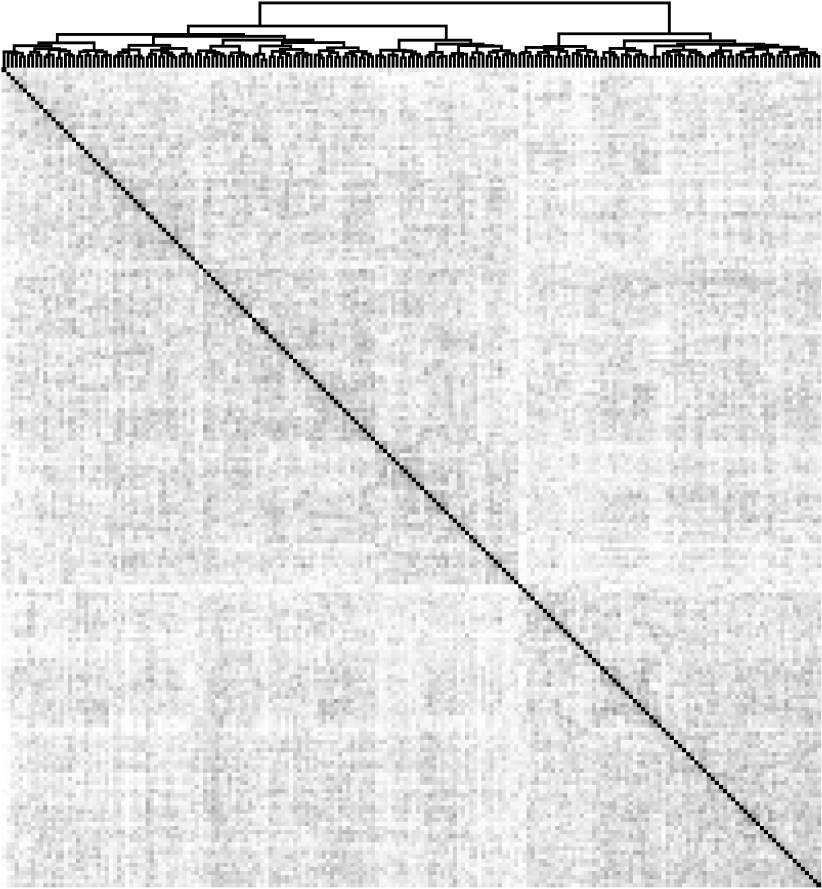
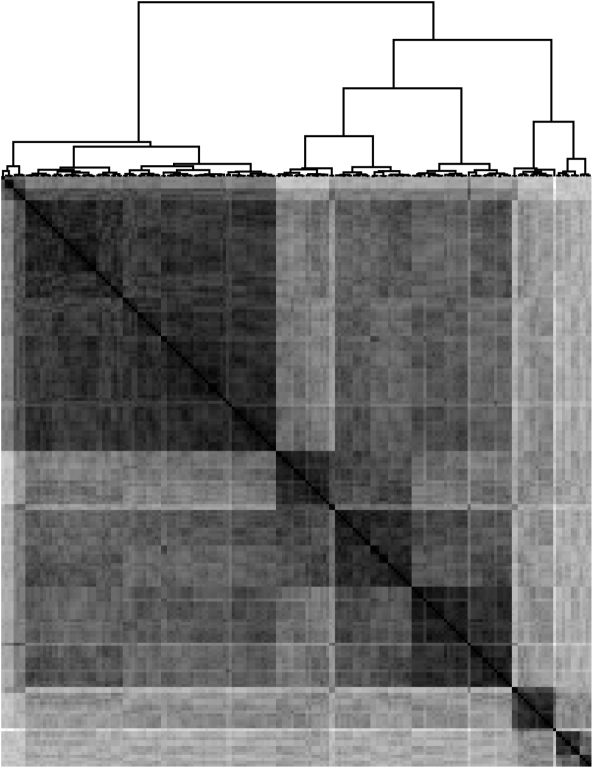
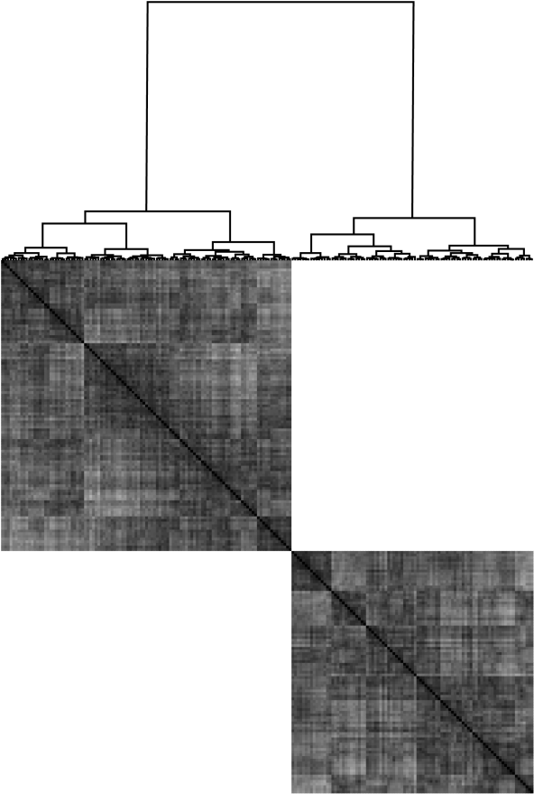
Figure 2: Examples for clustered overlap matrices with dendrograms showing the structures of the configurations space, each time 200 sampled for one realization ($L=16384,T=0.5$). A black dot means $q=1$ while white corresponds to $q=0$. Shown are (left) Hash with 90 lines; (middle) Mondrian with 90 lines; (right) Sierpinski triangles.

Each polymer configuration $P$ is characterized, first, by its energy $E(P)$ as defined above. This allows one to measure in equilibrium the average energy $\langle E\rangle$ and the specific heat $C(T)=(\langle E^{2}\rangle-\langle E\rangle^{2})/(NT^{2})$, for which one can also set up corresponding transfer-matrix equations Derrida and Golinelli (1990). For the random-disorder ensembles a linear average of all quantities over different realizations is performed, not indicated by separate brackets here. To characterize the model with respect to its energy landscape, the overlap $q$ between two polymers $P_{1},P_{2}$ is used Mukherji (1994), which is the fraction of joint sites, i.e., $q_{12}\equiv|P_{1}\cap P_{2}|/(2L+1)\in[0,1]$. By sampling many polymers in equilibrium, evaluating all (or many) overlaps, an approximation of the distribution $P(q)$ of overlaps is obtained.

To analyze the configuration space of these three ensembles, different disorder realization were studied first at temperature $T=0.5$. System sizes ranging from $L=64$ to $L=32768$ were considered. A number of independent disorder realizations ranging from 2000 for the smallest size to 500 for the largest size were investigated. For each disorder configuration $M=200$ independent polymer configurations were sampled in exact equilibrium.

The configuration space structure was analyzed by applying the an agglomerative clustering approach of Ward . The hierarchical structure obtained by the clustering can be visualized by a tree, usually called dendrogram, where each branching corresponds to a subspace of confirgurations, see Fig. 2. The sequence of configurations as located in the leafs defines a partial order. This order can be used to display the matrix of the pair-wise overlaps where the order of the rows and columns is exactly given by the leaf order, see also Fig. 2. For the Hash ensemble, a rather gray uniform area is visible. This indicates that the configuration space is rather uniform, like a paramagnet. On the other hand, the matrices for the samples from Mondrian and Sierpinski display a block-diagonal structure, which is recursively visible inside the blocks as well. This is an indication for a complex configuration space, as it has been observed, e.g., for mean-field spin glass models Katzgraber and Hartmann (2009) or solution-space landscapes of optimization problems Barthel and Hartmann (2004); Mann and Hartmann (2010).

Figure 3: Distribution $P(q)$ of overlaps at temperature $T=0.5$ for four different system sizes. The results are for (a) Hash, (b) Mondrian, and (c) Sierpinski triangles. In (d) the variance $\sigma^{2}_{q}$ of these distributions for the three ensembles is shown as function of the system size $N$, together with fits (see text).

In Fig. 3 the distributions of overlaps are shown. For the Hash case, the distribution gets strongly narrower, indicating a convergence to $P(q)=\delta(q-q_{0})$, which corresponds to a trivial configuration landscape. From a fit of the mean as function of $L$ to a power-law plus constant $q_{0}$, a value of $q_{0}=0.081(3)$ was obtained. On the other hand, for the other two ensembles $P(q)$ seems to converge to a broad distribution for $q>0$ plus a delta-peak at $q=0$ with some weight $w_{0}$, which accounts for polymers having different paths right from the start. For for the Sierpinski ensemble the data exhibits a convergence to $w_{0}=0.5$. This is compatible with the structure of the lattice, since at the starting site the paths either go down or right and never meet again, thus half of the pairs have zero overlap. For the Mondrian ensemble, a much smaller limiting zero-overlap peak-weight $w_{0}\approx 0.04$ is found, i.e., most of the overlap distribution is located in the non-trivial part. Also shown in Fig. 3 are the variances $\sigma_{q}^{2}$ of the distributions of overlaps for the three ensembles. For the Mondrian and the Sierpinski ensembles, the variance seems to converge to finite values in the $L\to\infty$ limit. This is confirmed by good fits for $L>100$ of the data to functions of the form $\sigma(N)=\sigma_{\infty}+aL^{-b}$ which lead to clear non-zero values $\sigma_{\infty}=0.1163(8)$ for the Sierpinski ensemble and $\sigma_{\infty}=0.0785(7)$ for the Mondrian ensemble. Thus, for these two ensembles the distribution of overlaps remains broad at low temperature in the thermodynamic limit $L\to\infty$ indicating a complex phase space structure. The variance for the Hash ensemble exhibits a positive curvature in the log-log plot, which could also be taken as indication for a complex structure. Nevertheless, here each polymer path can be decomposed in many sub paths with a high degree of independence, which speaks in favor of a simple configuration-space structure. Indeed, a limiting zero width is compatible: When fitting for $L>100$ a power-law with a correction term, $\tilde{\sigma}(N)=aL^{-b}(1+eL^{-d})$, a good fit is obtained as well, as shown in the figure.

Figure 4: (left) Sample distributions $P(K)$ of the ultrametricity measure for the Mondrian, and Hash ensembles. (Right) variance $\sigma^{2}_{K}$ of these distributions for the three ensembles as function of the system size $N$, together with fits (see text).

A hierarchical configuration space, like for the SK model, is characterized by an ultrametric structure Rammal et al. (1986), i.e., an underlying tree. To characterize ultrametricity, one considers triples of configurations $P_{1},P_{2},$ and $P_{3}$ and their mutual overlaps $q_{12},q_{13},$ and $q_{23}$ which are, without loss of generality, ordered such that $q_{12}\leq q_{13}\leq q_{23}$. For a true ultrametric space, for an infinite system size, $q_{12}=q_{13}$ would hold. To characterize the emergence of ultrametricity here, the quantity $K=(q_{13}-q_{12})/\sigma_{q}$ is used Katzgraber and Hartmann (2009), where $\sigma_{q}$ is the width of the overlap distribution $P(q)$. For a non-trivial ultrametric organization, the distribution $P(K)$ should converge to a delta-function $\delta(K)$, i.e., a variance $\sigma^{2}_{K}$ which converges to zero. In the left of Fig. 4 samples for $P(K)$ are shown for Mondrian and Hash ensembles. The former one exhibits a slight change towards smaller values of $K$ when increasing the system size $L$. For the latter one, the distribution is much broader, also for the largest considered size. This is confirmed by the behavior of the variance $\sigma_{K}^{2}$ of these distributions as function of the system size. The data is compatible with a gentle power-law decreases, shown as straight lines, for the Mondrian and the Sierpinski ensembles. This can be expected for the fractal Sierpinski ensemble since it has an obvious hierarchical structure. Note that the convergence even in this obvious ultrametric case is slow, as it was also observed for long-range spin glasses exhibiting RSB Katzgraber and Hartmann (2009). Thus, the data indicates that also the Mondrian ensemble exhibits ultrametricity as well. Also, the variance seems to converge to a constant for the Hash ensemble, compatible with the absence ultrametricity, and expected because of the simpler distribution of overlaps.

Figure 5: (left) Specific heat $C(T)$ as function of temperature for the Mondrian ensemble and four different system sizes. The inset shows the peak height $C_{\max}$ as function of the system size. (right) Position $T_{\max}$ of the peak of $C(T)$ as function of system size $L$ and in the inset the width $\sigma_{C}$ of the peak. The lines for $C(T)$ are guide to the eyes, the other lines display fits (see text).

In order to study the temperature dependence Derrida and Golinelli (1990) of an ensemble with complex behavior, for Mondrian, a large number of simulations was performed. Note that similar simulations for the Sierpinski model exhibited hard to analyze discotinuities and are thus not presented here. Lattice sizes $L\leq 16384$ for many temperatures $T\in[0.1,3]$, plus for $L=32768$ for few temperatures near the estimated critical point were considered with the number of disorder samples between 500 and 1000. In the left of Fig. 5 examples for the specific heat $C(T)$ behavior is shown. Clearly peaks are visible near $T\approx 1.4$, growing and narrowing with increasing system size, indicating a phase transition. For a second order phase transition Stanley (1971); Goldenfeld (1992); Cardy (1996); Yeomans (2002) one would expect that the specific heat scales as

$$C(T,L)=L^{\alpha/\nu}\tilde{c}((T-T_{c})L^{1/\nu})\,,$$ (1)

with a size-independent function $\tilde{c}()$ and critical exponents $\nu$, describing the divergence of the correlation length, and $\alpha$ describing the divergence of the specific heat. Indeed, the height of the peak follows clearly a power law $C_{\max}(L)\sim L^{\alpha/\nu}$, see inset of the left Fig. 5. A fit to this power law results in $\alpha/\nu=0.69(2)$.

The position $T_{\max}$ of the peak was estimated by fitting Gaussians near the peak. The position as a function of the system size is shown in the right of Fig. 5. Only a weak, third-digit significant, but non-monotonous size dependence is visible. Equation (1) means that scaling of the peak position leads to a leading behavior $T_{\max}(N)-T_{c}\sim L^{-1/\nu}$. Nevertheless, fitting just a power law does not work well, even when restricting to larger sizes. On the other hand, Eq. (1) also concerns the shape of the specific heat, i.e., the width of the peak region should also scale like $L^{-1/\nu}$. The width, as obtained also from the Gaussian fits, shows indeed a clear power law. A fit to a power law, yielded $\nu=-2.02(8)$. When fixing $\nu$ to this value, a fit to a power-law with correction $T_{\max}(N)=T_{c}+cL^{-1/\nu}(1+dL^{-\omega})$ yields a reasonable fit, see Fig. 5, with $T_{c}=1.439(8)$. With this value of $\nu$, a rather large value of $\alpha\approx 1.4$ results, which could indicate that actually a first-order phase transition is behind the seen data . This is compatible with the observed discontinities of the related Sierpinski lattice.

Figure 6: Mondrian ensemble and different system sizes in the (left) the mean overlap $q(T)$ as function of temperature. The inset shows the data near the estimated transition point, indicated by a vertical dashed line. (right) mean width $\sigma_{q}(T)$ of the overlap distribution, for three sample system sizes The inset shows the rescaled data for system sizes $L\geq 1024$.

The average overlap $q(T)$ is shown in the left of Fig. 6. At low temperatures $T>T_{c}$, the average overlap is non-zero. The curves for different system sizes cross near $T_{c}$ and just below $T_{c}$ the average overlap grows with the system size. This is an unusual behavior when comparing, e.g., with a ferromagnet. A data collapse (not shown) leads to an unphysical negative critical exponent. Note that also the average squared overlap (not shown) exhibits this behavior. The average width $\sigma_{q}(T)$ of the overlap distribution is shown in the right of Fig. 6. The data can be rescaled reasonably well, see inset, according to $\sigma_{q}(T,L)=L^{-\gamma/\nu}\tilde{\sigma}((T-T_{c})L^{1/\nu})$ when using the values $T_{c}=1.439$, $\nu=2.02$ obtained already and estimating $\gamma/\nu=0.07(2)$. The smallest system sizes are excluded from the collapse due to too large finite-size corrections. $L=32768$ is not included here due to bad statistics.

To conclude, it was shown that some specific ensembles of the disorder for random polymers on a two-dimensional lattice, at low temperatures exhibit a complex hierarchical organization of the phase space, similar to RSB. In contrast to other models exhibiting complex behavior, the present models allows for fast and exact sampling at arbitrary temperatures, i.e., to study large system in true equilibrium. This may open a path, by just using suitably correlated disorder ensembles, to study in a numerically convenient way complex behavior. This may be done for other disorder ensembles, other lattice dimensions or even other models where exact equilibrium sampling is possible.