Efficient Algorithms for Learning from Coarse Labels

Abstract

For many learning problems one may not have access to fine grained label information; e.g., an image can be labeled as husky, dog, or even animal depending on the expertise of the annotator. In this work, we formalize these settings and study the problem of learning from such coarse data. Instead of observing the actual labels from a set $\mathcal{Z}$, we observe coarse labels corresponding to a partition of $\mathcal{Z}$ (or a mixture of partitions).

Our main algorithmic result is that essentially any problem learnable from fine grained labels can also be learned efficiently when the coarse data are sufficiently informative. We obtain our result through a generic reduction for answering Statistical Queries (SQ) over fine grained labels given only coarse labels. The number of coarse labels required depends polynomially on the information distortion due to coarsening and the number of fine labels $|\mathcal{Z}|$.

We also investigate the case of (infinitely many) real valued labels focusing on a central problem in censored and truncated statistics: Gaussian mean estimation from coarse data. We provide an efficient algorithm when the sets in the partition are convex and establish that the problem is NP-hard even for very simple non-convex sets.

1 Introduction

Supervised learning from labeled examples is a classical problem in machine learning and statistics: given labeled examples, the goal is to train some model to achieve low classification error. In most modern applications, where we train complicated models such as neural nets, large amounts of labeled examples are required. Large datasets such as Imagenet, [RDS⁺15], often contain thousands of different categories such as animals, vehicles, etc., each one of those containing many fine grained subcategories: animals may contain dogs and cats and dogs may be further split into different breeds etc. In the last few years, there have been many works that focus on fine grained recognition, [GLB⁺18, CDCM18, TSD⁺20, QCJ⁺20, LGW17, JLYW19, JLL⁺20, BSS⁺20, TKD⁺19]. Collecting a sufficient amount of accurately labeled training examples is a hard and expensive task that often requires hiring experts to annotate the examples. This has motivated the problem of learning from coarsely labeled datasets, where a dataset is not fully annotated with fine grained labels but a combination of fine, e.g., cat, and coarse labels, e.g., animal, is given, [DKFF13, RGGV15].

Inference from coarse data naturally arises also in unsupervised, i.e., distribution learning settings: instead of directly observing samples from the target distribution, we observe “representative” points that correspond to larger sets of samples. For example, instead of observing samples from a real valued random variable, we round them to the closest integer. An important unsupervised problem that fits in the coarse data framework is censored statistics, [Coh16, Wol79, B⁺96, Sch86]. Interval censoring, that arises in insurance adjustment applications, corresponds to observing points in some interval and point masses at the endpoints of the interval instead of observing fine grained data from the whole real line. Moreover, the problem of learning the distribution of the output of neural networks with non-smooth activations (e.g., ReLU networks, [WDS19]) also fits in our model of distribution learning with coarse data, see Figure 1(c).

Even though the problem of learning from coarsely labeled data has attracted significant attention from the applied community, from a theoretical perspective little is known. In this work, we provide efficient algorithms that work in both the supervised and the unsupervised coarse data settings.

1.1 Our Model and Results

We start by describing the generative model of coarsely labeled data in the supervised setting. We model coarse labels as subsets of the domain of all possible fine labels. For example, assume that we hire an expert on dog breeds and an expert on cat breeds to annotate a dataset containing images of dogs and cats. With probability $1/2$, we get samples labeled by the dog expert, i.e., labeled according to the partition

$$\{\mathrm{cat}=\{\mathrm{persian~{}cat},\mathrm{bengal~{}cat},\ldots\},\{\mathrm{maltese~{}dog}\},\{\mathrm{husky~{}dog}\},\ldots\ \}\,.$$

On the other hand, the cat expert will provide a fine grained partition over cat breeds and will group together all dog breeds. Our coarse data model captures exactly this mixture of different label partitions.

Definition 1 (Generative Process of Coarse Data with Context).

Let $\mathcal{X}$ be an arbitrary domain, and let $\mathcal{Z}=\{1,\ldots,k\}$ be the discrete domain of all possible fine labels. We generate coarsely labeled examples as follows:

1. Draw a finely labeled example $(x,z)$ from a distribution $\mathcal{D}$ on $\mathcal{X}\times\mathcal{Z}$.

2. Draw a coarsening partition $\mathcal{S}$ (of $\mathcal{Z}$) from a distribution $\pi$.

3. Find the unique set $S\in\mathcal{S}$ that contains the fine label $z$.

4. Observe the coarsely labeled example $(x,S)$.

We denote $\mathcal{D}_{\pi}$ the distribution of the coarsely labeled example $(x,S)$.

In the supervised setting, our main focus is to answer the following question.

Question 1.

Can we train a model, using coarsely labeled examples $(x,S)\sim\mathcal{D}_{\pi}$, that classifies finely labeled examples $(x,z)\sim\mathcal{D}$ with accuracy comparable to that of a classifier that was trained on examples with fine grained labels?

Definition 1 does not impose any restrictions on the distribution over partitions $\pi$. It is clear that if partitions are very rough, e.g., we split $\mathcal{Z}$ into two large disjoint subsets, we lose information about the fine labels and we cannot hope to train a classifier that performs well over finely labeled examples. In order for 1 to be information theoretically possible, we need to assume that the partition distribution $\pi$ preserves fine-label information. The following definition quantifies this by stating that reasonable partition distributions $\pi$ are those that preserve the total variation distance between different distributions supported on the domain of the fine labels $\mathcal{Z}$. We remark that the following definition does not require $\mathcal{D}$ to be supported on pairs $(x,z)$ but is a general statement for the unsupervised version of the problem, see also Definition 6.

Definition 2 (Information Preserving Partition Distribution).

Let $\mathcal{Z}$ be any domain and let $\alpha\in(0,1]$. We say that $\pi$ is an $\alpha$-information preserving partition distribution if for every two distributions $\mathcal{D}^{1},\mathcal{D}^{2}$ supported on $\mathcal{Z}$, it holds that $\mathrm{TV}(\mathcal{D}^{1}_{\pi},\mathcal{D}^{2}_{\pi})\geq\alpha\cdot\mathrm{TV}(\mathcal{D}^{1},\mathcal{D}^{2})$, where $\mathrm{TV}(\mathcal{D}^{1},\mathcal{D}^{2})$ is the total variation distance of $\mathcal{D}^{1}$ and $\mathcal{D}^{2}$.

For example, the partition distribution defined in the dog/cat dataset scenario, discussed before Definition 1, is $1/2$-information preserving, since we observe fine labels with probability $1/2$. In this case, it is easy, at the expense of losing the statistical power of the coarse labels, to combine the finely labeled examples from both experts in order to obtain a dataset consisting only of fine labels. However, our model allows the partitions to have arbitrarily complex combinatorial structure that makes the process of “inverting” the partition transformation computationally challenging. For example, specific fine labels may be complicated functions of coarse labels: “medium sized” and “pointy ears” and “blue eyes” may be mapped to the “husky dog” fine label.

Our first result is a positive answer to 1 in essentially full generality: we show that concept classes that are efficiently learnable in the Statistical Query (SQ) model, [Kea98], are also learnable from coarsely labeled examples. Our result is similar in spirit with the result of [Kea98], where it is proved that SQ learnability implies learnability under random classification noise.

Informal Theorem 1 (SQ Learnability implies Learnability from Coarse Examples).

Any concept class $\mathcal{C}$ that is efficiently learnable with $M$ statistical queries from finely labeled examples $(x,z)\sim\mathcal{D}$, can be efficiently learned from $O(\mathrm{poly}(k/\alpha))\cdot M$ coarsely labeled examples $(x,S)\sim\mathcal{D}_{\pi}$ under any $\alpha$-information preserving partition distribution $\pi$.

Statistical Queries are queries of the form $\operatorname*{\mathbf{E}}_{(x,z)\sim\mathcal{D}}[q(x,z)]$ for some query function $q(x,z)$. It is known that almost all known machine learning algorithms [AD98, BFKV98, BDMN05, DV08, BF15, FGR⁺17] can be implemented in the SQ model. In particular, in [FGV17], it is shown that (Stochastic) Gradient Descent can be simulated by statistical queries. This implies that our result can be applied, even in cases where it is not possible to obtain formal optimality guarantees, e.g., training deep neural nets. We can train such models using coarsely labeled data and guarantee the same performance as if we had direct access to fine labels (see also Appendix A). As another application, we consider the problem of multiclass logistic regression with coarse labels. It is known, see e.g., [FHT⁺01], that given finely labeled examples $(x,z)\sim\mathcal{D}$, the likelihood objective for multiclass logistic regression is concave with respect to the weight matrix. Even though the likelihood objective is no-longer concave when we consider coarsely labeled examples $(x,S)\sim\mathcal{D}_{\pi}$, our theorem bypasses this difficulty and allows us to efficiently perform multiclass logistic regression with coarse labels.

Formally, we design an algorithm (Algorithm 1) that, given coarsely labeled examples $(x,S)$, efficiently simulates statistical queries over finely labeled examples $(x,z)$. Surprisingly, the runtime and sample complexity of our algorithm do not depend on the combinatorial structure of the partitions, but only on the number of fine labels $k$ and the information preserving parameter $\alpha$ of the partition distribution $\pi$.

Theorem 3 (SQ from Coarsely Labeled Examples).

Consider a distribution $\mathcal{D}_{\pi}$ over coarsely labeled examples in $\mathbb{R}^{d}\times[k]$, (see Definition 1) with $\alpha$-information preserving partition distribution $\pi$. Let $q:\mathbb{R}^{d}\times[k]\to[-1,1]$ be a query function, that can be evaluated on any input in time $T$, and $\tau,\delta\in(0,1)$. There exists an algorithm (Algorithm 1), that draws $N=\widetilde{O}(k^{4}/(\tau^{3}\alpha^{2})\log(1/\delta))$ coarsely labeled examples from $\mathcal{D}_{\pi}$ and, in $\mathrm{poly}(N,T)$ time, computes an estimate $\hat{r}$ such that, with probability at least $1-\delta$, it holds $\big{|}\operatorname*{\mathbf{E}}_{(x,z)\sim\mathcal{D}}[q(x,z)]-\hat{r}\big{|}\leq\tau\,.$

Learning Parametric Distributions from Coarse Samples.

In many important applications, instead of a discrete distribution over fine labels, a continuous parametric model is used. A popular example is when the domain $\mathcal{Z}$ of Definition 1 is the entire Euclidean space $\mathbb{R}^{d}$, and the distribution of finely labeled examples is a Gaussian distribution whose parameters possibly depend on the context $x$. Such censored regression settings are known as Tobit models [Tob58, Mad86, Gou00]. Lately, significant progress has been made from a computational point of view in such censored/truncated settings in the distribution specific setting, e.g., when the underlying distribution is Gaussian [DGTZ18, KTZ19], mixtures of Gaussians [NP19], linear regression [DGTZ19, IZD20, DRZ20]. In this distribution specific setting, we consider the most fundamental problem of learning the mean of a Gaussian distribution given coarse data.

Definition 4 (Coarse Gaussian Data).

Consider the Gaussian distribution $\mathcal{N}(\bm{\mu}^{\star})$, with mean $\bm{\mu}^{\star}\in\mathbb{R}^{d}$ and identity covariance matrix. We generate a sample as follows:

1. Draw $\bm{z}$ from $\mathcal{N}(\bm{\mu}^{\star})$.

2. Draw a partition $\mathcal{S}$ (of $\mathbb{R}^{d}$) from $\pi$.

3. Observe the set $S\in\mathcal{S}$ that contains $\bm{z}$.

We denote the distribution of $S$ as $\mathcal{N}_{\pi}(\bm{\mu}^{\star})$.

Remark 1.

We remark that we only require membership oracle access to the subsets of the partition $\mathcal{S}$. A set $S\subseteq\mathbb{R}^{d}$ corresponds to a membership oracle $\mathcal{O}_{S}:\mathbb{R}^{d}\to\{0,1\}$ that given $\bm{x}\in\mathbb{R}^{d}$ outputs whether the point lies inside the set $S$ or not.

We first study the above problem, from a computational viewpoint. For the corresponding problems in censored and truncated statistics no geometric assumptions are required for the sets: in [DGTZ18] it was shown that an efficient algorithm exists for arbitrarily complex truncation sets. In contrast in our more general model of coarse data we show that having sets with geometric structure is necessary. In particular we require that every set of the partition is convex, see Figure 1(b,c). We show that when the convexity assumption is dropped, learning from coarse data is a computationally hard problem even under a mixture of very simple sets.

Theorem 5 (Hardness of Matching the Observed Distribution with General Partitions).

Let $\pi$ be a general partition distribution. Unless $\textsc{RP}=\textsc{NP}$, no algorithm with sample access to $\mathcal{N}_{\pi}({\bm{\mu}}^{\star}),$ can compute, in $\mathrm{poly}(d)$ time, a $\widetilde{\bm{\mu}}\in\mathbb{R}^{d}$ such that $\mathrm{TV}(\mathcal{N}_{\pi}(\widetilde{\bm{\mu}}),\mathcal{N}_{\pi}(\bm{\mu}^{\star}))<1/d^{c}$ for some absolute constant $c>1$.

We prove our hardness result using a reduction from the well known Max-Cut problem, which is known to be NP-hard, even to approximate [Hås01]. In our reduction, we use partitions that consist of simple sets: fat hyperplanes, ellipsoids and their complements: the computational hardness of this problem is rather inherent and not due to overly complicated sets.

(a) Non-Identifiable Case

(b) Convex Partition Case

(c) ReLU Case

Figure 1: (a) is a very rough partition, that makes learning the mean impossible: Gaussians $\mathcal{N}((0,z))$ centered along the same vertical line $(0,z)$ assign exactly the same probability to all cells of the partitions and therefore, $\mathrm{TV}(\mathcal{N}_{\pi}((0,z_{1})),\mathcal{N}_{\pi}((0,z_{2})))=0$: it is impossible to learn the second coordinate of the mean. (b) is a convex partition of $\mathbb{R}^{2}$, that makes recovering the Gaussian possible. (c) is the convex partition corresponding to the output distribution of one layer ReLU networks. When both coordinates are positive, we observe a fine sample (black points correspond to singleton sets). When exactly one coordinate (say $\bm{x}_{1}$) is positive, we observe the line $L_{z}=\{\bm{x}:\bm{x}_{2}<0,\bm{x}_{1}=z>0\}$ that corresponds to the ReLU output $(\bm{x}_{1},0)$. If both coordinates are negative, we observe the set $\{\bm{x}:\bm{x}_{1}<0,\bm{x}_{2}<0\}$, that corresponds to the point $(0,0)$.

On the positive side, we identify a geometric property that enables us to design a computationally efficient algorithm for this problem: namely we require all the sets of the partitions to be convex, e.g., Figure 1(b,c). We remark that having finite or countable subsets, is not a requirement of our model. For example, we can handle convex partitions of the form (c) that correspond to the output distribution of a ReLU neural network, see [WDS19]. We continue with our theorem for learning Gaussians from coarse data.

Informal Theorem 2 (Gaussian Mean Estimation with Convex Partitions).

Let $\epsilon\in(0,1)$. Consider the generative process of coarse $d$-dimensional Gaussian data $\mathcal{N}_{\pi}(\bm{\mu}^{\star})$. Assume that the partition distribution $\pi$ is $\alpha$-information preserving and is supported on convex partitions of $\mathbb{R}^{d}$. Then, the empirical log-likelihood objective

$$\mathcal{L}_{N}(\bm{\mu})=\frac{1}{N}\sum_{i=1}^{N}\log\mathcal{N}(\bm{\mu};S_{i})$$

is concave with respect to $\bm{\mu}$ for $S_{i}\sim\mathcal{N}_{\pi}(\bm{\mu}^{\star})$. Moreover, it suffices to draw $N=\widetilde{O}(d/(\epsilon^{2}\alpha^{2}))$ samples from $\mathcal{N}_{\pi}(\bm{\mu}^{\star})$ so that the maximizer $\widetilde{\bm{\mu}}$ of the empirical log-likelihood satisfies

$$\mathrm{TV}(\mathcal{N}(\widetilde{\bm{\mu}}),\mathcal{N}(\bm{\mu}^{\star}))\leq\epsilon\,,$$

with probability at least $99\%$.

Our algorithm for mean estimation of a Gaussian distribution relies on the log-likelihood being concave when the partitions are convex. We remark that, similar to our approach, one can use the concavity of likelihood to get efficient algorithms for regression settings, e.g., Tobit models, where the mean of the Gaussian is given by a linear function of the context $\bm{A}\bm{x}$ for some unknown matrix $\bm{A}$.

1.2 Related Work

Our work is closely related to the literature of learning from censored-truncated data and learning with noise. There has been a large number of recent works dealing inference with truncated data from a Gaussian distribution [DGTZ18, KTZ19], mixtures of Gaussians [NP19], linear regression [DGTZ19, IZD20, DRZ20], sparse Graphical models [BDNP21] or Boolean product distributions [FKT20], and non-parametric estimation [DKTZ21]. A significant feature of our work is that it can capture the closely related field of censored statistics [Coh16, B⁺96, Wol79].

The area of robust statistics [Hub04] is also very related to our work as it also deals with biased data-sets and aims to identify the distribution that generated the data. Recently, there has been a large volume of theoretical work for computationally-efficient robust estimation of high-dimensional distributions [DKK⁺16, CSV17, LRV16, DKK⁺17, DKK⁺18, KKM18, HL19, DKK⁺19, CDGS20, BDH⁺20] in the presence of arbitrary corruptions to a small $\varepsilon$ fraction of the samples.

The line of research dealing with statistical queries [Kea98, BFKV98, FPV15, FGV17, Fel17, FGR⁺17, DKS17, DKKZ20] is closely related to one of our main results (Theorem 3). It is generally believed that SQ algorithms capture all reasonable machine learning algorithms [AD98, BFKV98, BDMN05, DV08, FGR⁺17, BF15, FGV17] and there is a rich line of research indicating SQ lower-bounds for these classes of algorithms [FGR⁺17, DKS17, Sha18, VW19, DKKZ20, DKZ20, GGJ⁺20, GGK20].

Learning from coarse labels is also referred in the ML literature as Partial Label Learning  [CST11a, CPCP14, YZ16a] (a weakly supervised learning problem where each training example is associated with a set of candidate labels among which only one is true). We refer to Appendix D for an extensive discussion.

2 Notation and Preliminaries

We let $[n]=\{1,\ldots,n\}$ and $[0..n]=\{0,\ldots,n\}$. We use lowercase bold letters $\bm{x}$ to denote vectors and capital bold letters $\bm{X}$ for matrices. We let $\bm{x}_{i}$ be the $i$-th coordinate of $\bm{x}$. We let $\|\bm{x}\|_{p}$ denote the $L_{p}$ norm of $\bm{x}$. We denote the indicator function $\bm{1}_{S}(\bm{x})=\bm{1}\{\bm{x}\in S\}$ for some set $S\subseteq\mathbb{R}^{d}$. We let $\mathrm{sgn}(\cdot)$ denote the sign function and we slightly overload the notation as follows: $\mathrm{sgn}:\mathbb{R}^{d}\to\{-1,+1\}^{d}$ stands for the sign function applied to each coordinate of a vector $\bm{x}\in\mathbb{R}^{d}$. For a graph $G$, we usually let $\bm{L}_{G}$ denote its Laplacian matrix. We denote $\mathcal{B}(\bm{x},\rho)$ the Euclidean ball of radius $\rho$ centered at $\bm{x}$; we simply refer to $\mathcal{B}$ if the radius and the center are clear from the context and we denote the associated sphere $\partial\mathcal{B}$, i.e., its boundary. The probability simplex is denoted by $\Delta^{n}$ and discrete distributions $\mathcal{D}$ supported on $[n]$ will usually be represented by their associated probability vectors $\bm{p}\in\Delta^{n}$. For any distribution $\mathcal{D}$, we overload the notation and we use the same notation for the corresponding density and denote $\mathcal{D}(S)=\sum_{x\in S}\mathcal{D}(x)$ for any $S\subseteq[n]$. We denote the support of the probability distribution $\mathcal{D}$ by $\mathrm{supp}(\mathcal{D})$. The $d$-dimensional Gaussian distribution will be denoted by $\mathcal{N}(\bm{\mu},\bm{\Sigma})$. When the covariance matrix is known, we simplify to $\mathcal{N}(\bm{\mu})$. For a set $S\subseteq\mathbb{R}^{d},$ we let $\mathcal{N}_{S}$ denote the conditional Gaussian distribution on the set $S$, i.e., $\mathcal{N}_{S}(\bm{\mu},\bm{\Sigma};\bm{x})=\bm{1}\{\bm{x}\in S\}\mathcal{N}(\bm{\mu},\bm{\Sigma};\bm{x})/\mathcal{N}(\bm{\mu},\bm{\Sigma};S)$. We denote $\Phi$ (resp. $\phi$) the cdf (resp. pdf) of the standard Normal distribution. The total variation distance of $\bm{p},\bm{q}\in\Delta^{n}$ is $\mathrm{TV}(\bm{p},\bm{q})=\max_{S\subseteq[n]}\bm{p}(S)-\bm{q}(S)=\|\bm{p}-\bm{q}\|_{1}/2$. For a random variable $x$, we let $\operatorname*{\mathbf{E}}[x],\operatorname*{\mathbf{V}}(x),\mathop{\mathbf{Cov}}(x)$ be the expected value, the variance and the covariance of $x$. For a joint distribution $\mathcal{D}$ of two random variables $x$ and $z$ over the space $\mathcal{X}\times\mathcal{Z}$, we let $\mathcal{D}_{x}$ (resp. $\mathcal{D}_{z}$) be the marginal distribution of $x$ (resp. $z$). Let $\mathcal{D}$ be a joint distribution over labeled examples $\mathcal{X}\times\mathcal{Z}$, with $\mathcal{X}$ be the input space and $\mathcal{Z}$ the label space. A statistical query (SQ) oracle $\mathrm{STAT}(\mathcal{D},\tau)$ with tolerance parameter $\tau\in[0,1]$ takes as input a statistical query defined by a real-valued function $q:\mathcal{X}\times\mathcal{Z}\rightarrow[-1,1]$ and outputs an estimate of $\operatorname*{\mathbf{E}}_{(x,z)\sim\mathcal{D}}[q(x,z)]$ that is accurate to within an additive $\pm\tau$.

3 Supervised Learning from Coarse Data

In this section, we consider the problem of supervised learning from coarse data. In this setting, there exists some underlying distribution over finely labeled examples, $\mathcal{D}$. However, we have sample access only to the distribution associated with coarsely labeled examples $\mathcal{D}_{\pi}$, see Definition 1. As discussed in Section 1, under this setting, even problems that are naturally convex when we have access to examples with fine labels, become non-convex when we introduce coarse labels (e.g., multiclass logistic regression). The main result of this section is Theorem 3, which allows us to compute statistical queries over finely labeled examples.

3.1 Overview of the Proof of Theorem 3

In order to simulate a statistical query we take a two step approach. Our first building block considers the unsupervised version of the problem, see Definition 6, i.e., we marginalize the context $x$ and try to learn the distribution of the fine labels $z$ given coarse samples $S$. This can be viewed as learning a general discrete distribution supported on $\mathcal{Z}=\{1,\ldots,k\}$ given coarse samples, i.e., subsets of $\mathcal{Z}$. We show that, when the partition distribution $\pi$ is $\alpha$-information preserving, this can be done efficiently, see Proposition 7. Our algorithm (Algorithm 1) exploits the fact that even though in general having coarse data results in non-concave likelihood objectives, when we consider parametric models (see, for example, the case of logistic regression in Appendix B), this is not true when we maximize over all discrete distributions. In Proposition 7, we show that $\widetilde{O}(k/(\epsilon\alpha)^{2})$ samples are sufficient for this step. For the details of this step, see Section 3.2.

Using the above algorithm, one could try to separately learn the marginal distribution over $x$, $\mathcal{D}_{x}$ and the distribution of the fine labels $z$ conditional on some fixed $x$; let us denote this distribution as $\mathcal{D}_{z}^{x}$. Then one could generate finely labeled examples $(x,z)$ and use them to estimate the query $\operatorname*{\mathbf{E}}_{(x,z)\sim\mathcal{D}}[q(x,z)]$. The reason that this naive approach fails is that it requires many coarse examples $(x,S)$ with exactly the same value of $x$. Unless the domain $\mathcal{X}$ is very small, the probability that we observe samples with the same value of $x$ is going to be tiny. In order to overcome this obstacle, at a high level, our approach is to split the domain $\mathcal{X}$ into larger sets and then, learn the conditional distribution of the labels, not on a fixed point $x$, but on these larger sets of non-trivial mass.

Intuitively, in order to have an effective partition of the domain $\mathcal{X}$, we want to group together points $x$ whose values $q(x,z)$ are close. Since $z$ belongs in a discrete domain $\mathcal{Z}=[k]$, we can decompose the query $q(x,z)$ as $q(x,z)=\sum_{i=1}^{k}q(x,i)\bm{1}\{z=i\}$. We estimate the value of $\operatorname*{\mathbf{E}}_{(x,z)\sim\mathcal{D}}[q(x,i)\bm{1}\{z=i\}]$ separately. To find a suitable reweighting of the domain $\mathcal{X}$, we perform rejection sampling, accepting a pair $(x,S)\sim\mathcal{D}$ with probability $q(x,i)$ : points $x$ that have small value $q(x,i)$ contribute less in the expectation and are less likely to be sampled. After performing this rejection sampling process based on $x$, we have pairs $(x,S)$, conditional that $x$ was accepted. Now, using our previous maximum likelihood learner of Proposition 7 we learn the marginal distribution over fine labels and use it to answer the query. We provide the details of this rejection sampling step in the full proof of Theorem 3, see Section 3.3.

For a description of the corresponding algorithm that simulates statistical queries, see Algorithm 1. To keep the presentation simple we state the algorithm for the case where the query function $q(x,z)$ is positive. It is straightforward to generalize it for general queries, see Section 3.3.

Algorithm 1 Statistical Queries from Coarse Labels.

1:Input: Query $q:\mathcal{X}\times\mathcal{Z}\mapsto(0,1]$, tolerance $\tau\in[0,1]$, confidence $\delta\in[0,1]$.

2:Oracle: Access to coarsely labeled samples $(x,S)\sim\mathcal{D}_{\pi}$, $\pi$ is $\alpha$-information preserving.

3:Output: Estimate $\widehat{r}$ such that $\big{|}\operatorname*{\mathbf{E}}_{(x,z)\sim\mathcal{D}}[q(x,z)]-\widehat{r}\big{|}\leq\tau$ with probability at least $1-\delta$.

4:procedure StatQuery($q,\tau,\delta$)

5:     Compute $\widehat{r}_{i}\leftarrow\mathrm{SQ}(q,i,O(\tau/k),\delta/k)$ for any $i\in\mathcal{Z}$.

6:     Output $\widehat{r}\leftarrow\sum_{i=1}^{k}\widehat{r}_{i}$.

7:procedure SQ($q,i,\rho,\delta$)

8:     Draw $N_{1}=\widetilde{\Theta}\big{(}\frac{\log(1/\delta)}{\rho^{2}}\big{)}$ samples $(x_{j},S_{j})$ from $\mathcal{D}_{\pi}$.

9:     Compute $\widehat{\mu}_{i}\leftarrow\frac{1}{N_{1}}\sum_{j=1}^{N_{1}}q(x_{j},i)$.

10:     if $\widehat{\mu}_{i}\leq\rho$ do

11:         Output $\widehat{r}_{i}\leftarrow 0$.

12:     end

13:     Draw $N_{2}=\widetilde{\Theta}\big{(}\frac{k\log(1/\delta)}{\rho^{3}\alpha^{2}}\big{)}$ samples $(x_{j},S_{j})$ from $\mathcal{D}_{\pi}$. $\triangleright$ $\widetilde{\Theta}\big{(}\frac{k^{4}\log(1/\delta)}{\tau^{3}\alpha^{2}}\big{)}$ examples overall.

14:     $T_{accept}\leftarrow\emptyset$. $\triangleright$ Training set of accepted samples.

15:     Add $S_{j}$ in $T_{accept}$ with probability $q(x_{j},i)$, $\forall j\in[N_{2}]$. $\triangleright$ Rejection Sampling Process.

16:     Compute $\widetilde{\mathcal{D}}$ using Proposition 7 with input $(T_{accept},\rho,\delta).$

17:     Output $\widehat{r}_{i}\leftarrow\widehat{\mu}_{i}\cdot\widetilde{\mathcal{D}}(i)$.

Remark 2 (Empirical Likelihood Approach).

One could try to use the empirical likelihood directly over the coarsely labeled data (as defined in [Owe01]). However, in general, these empirical likelihood objectives are non-convex when the data are coarse and therefore it is computationally hard to optimize them directly. Our approach for simulating statistical queries consists of two ingredients: reweighting the feature space via rejection sampling in order to group together points and learning discrete distributions from coarse data. To learn the discrete distributions (Section 3.2), we use a (direct) empirical likelihood approach similar to that of  [Owe88, O⁺90, Owe01]. However, our main contribution is the use of rejection sampling to reduce the initial non-convex problem to the special case of learning a discrete distribution (with small support) from coarse data which, as we prove, is a tractable (convex) problem. For more connections with censored statistics techniques, we refer the reader to [TG75, Owe88, GVDLR97, Owe01].

3.2 Learning Marginals Over Fine Labels

In this subsection, we deal with unsupervised learning from coarse data in discrete domains. Although this is an ingredient of our main result for simulating statistical queries in a supervised setting where labeled data $(x,S)$ are given, the result of this section does not depend on the points $x$ and concerns the unsupervised version of the problem. To keep the notation simple, we will use $\mathcal{D}$ to denote a distribution over finite labels $\mathcal{Z}$.

Definition 6 (Generative Process of Coarse Data).

Let $\mathcal{Z}$ be a discrete domain and $\mathcal{D}$ be a distribution supported on $\mathcal{Z}$. Moreover, let $\pi$ be a distribution supported on partitions of $\mathcal{Z}$. We consider the following generative process:

1. Draw $z$ from $\mathcal{D}$.

2. Draw a partition $\mathcal{S}$ from the distribution over all partitions $\pi$.

3. Observe the set $S\in\mathcal{S}$ that contains $z$.

We denote the distribution of $S$ as $\mathcal{D}_{\pi}$.

The assumption that we require is that the partition distribution $\pi$ is $\alpha$-information preserving, see Definition 2. At this point we give some examples of information preserving partition distributions. We first observe that $\alpha=0$ if and only if the problem is not identifiable. For instance, if $\pi$ is supported only on the partition $\mathcal{S}=\{\{1,2\},\{3,\ldots,k\}\}$, the problem is not identifiable, since, for example, the fine label $1$ is indistinguishable from the fine label $2$. The value $\alpha=1$ is attained when the partition totally preserves the distribution distance. Intuitively, the value $1-\alpha$ corresponds to the distortion that the coarse labeling introduces to a finely labeled dataset.

In many cases most fine labels may be missing. Consider two data providers that use different methods to round their samples. The rounding’s uncertainty can be viewed as a coarse labeling of the data. Assume that we add discrete (balanced Bernoulli) noise $\xi$ to some true value $x\in[0..k]$. Consider two partitions $\{\mathcal{S}_{1},\mathcal{S}_{2}\}$ with $\mathcal{S}_{1}=\{\{0,1\},\{2,3\},\dots,\{k-1,k\},\{k+1\}\}$ and $\mathcal{S}_{2}=\{\{0\},\{1,2\},\dots\{k-1,k\}\}$. Observe that, when $x+\xi$ is odd, we can think of the rounded sample, as a draw from $\mathcal{S}_{1}$ and when $x+\xi$ is even, as a draw from $\mathcal{S}_{2}$. This example shows that we can capture the problem of deconvolution of two distributions $\mathcal{D}_{1},\mathcal{D}_{2}$, where one of them is known and we observe samples $x_{1}+x_{2},x_{i}\sim\mathcal{D}_{i}$.

The following proposition establishes the sample complexity of unsupervised learning of discrete distributions with coarse data. Our goal is to compute an estimate of the discrete distribution $\mathcal{D}^{\star}$ with probability vector $\bm{p}^{\star}\in\Delta^{k}$ from $N$ coarse samples $S_{1},\dots,S_{N}$ drawn from the distribution $\mathcal{D}_{\pi}^{\star}$. Our algorithm maximizes the empirical likelihood. Analyzing the empirical log-likelihood objective $\mathcal{L}_{N}(\bm{p})=\frac{1}{N}\sum_{n=1}^{N}\log\big{(}\sum_{i\in S_{n}}\bm{p}_{i}\big{)}$, where $\bm{p}\in\Delta^{k}$ is a guess probability vector, we observe that the problem is concave and, therefore, can be efficiently optimized (e.g., by gradient descent).

Proposition 7.

Let $\mathcal{Z}$ be a discrete domain of cardinality $k$ and let $\mathcal{D}$ be a distribution supported on $\mathcal{Z}$. Moreover, let $\pi$ be an $\alpha$-information preserving partition distribution for some $\alpha\in(0,1]$. Then, with $N=\widetilde{O}(k/(\epsilon^{2}\alpha^{2})\log(1/\delta))$ samples from $\mathcal{D}_{\pi}$ and in time polynomial in the number of samples $N$, we can compute a distribution $\widetilde{\mathcal{D}}$ supported on $\mathcal{Z}$ such that $\mathrm{TV}(\widetilde{\mathcal{D}},\mathcal{D})\leq\epsilon$.

Proof.

Let $\mathcal{D}^{\star}$ be the target discrete distribution, supported on a discrete domain of size $k$, and let $\bm{p}^{\star}\in\Delta^{k}$ be the corresponding probability vector. For some distribution $\mathcal{D}$ supported on a discrete domain of size $k$, we define the following population log-likelihood objective.

$$\mathcal{L}(\mathcal{D})=\operatorname*{\mathbf{E}}_{S\sim\mathcal{D}^{\star}_{\pi}}[\log\mathcal{D}(S)]=\operatorname*{\mathbf{E}}_{S\sim\mathcal{D}^{\star}_{\pi}}\Big{[}\log\big{(}\sum_{i\in S}\mathcal{D}(i)\big{)}\Big{]}\,.$$ (3.1)

Since $\mathcal{D}$ is a discrete distribution for simplicity we may identify with its probability vector $\bm{p}$, where $\bm{p}_{i}=\mathcal{D}(i)$. Therefore, for any $\bm{p}$ in the probability simplex $\Delta^{k}$, we define

$$\mathcal{L}(\bm{p})=\operatorname*{\mathbf{E}}_{S\sim\mathcal{D}^{\star}_{\pi}}\Big{[}\log\sum_{i\in S}\bm{p}_{i}\Big{]}\,.$$ (3.2)

The corresponding empirical log-likelihood objective after drawing $N$ independent samples $S_{1},\ldots,S_{N}$ from $\mathcal{D}_{\pi}^{\star}$ is given by

$$\mathcal{L}_{N}(\bm{p})=\frac{1}{N}\sum_{n=1}^{N}\log\left(\sum_{i\in S_{n}}\bm{p}_{i}\right)\,.$$ (3.3)

We first observe that the log-likelihood (both the population and the empirical) is a concave function and therefore can be efficiently optimized (e.g., by gradient descent). Thus, our main focus in this proof is to bound its sample complexity. We first observe that when the guess $\bm{p}\in\Delta^{k}$ has some very biased coordinates, i.e., for some subset $S$ the corresponding $\bm{p}_{i}$’s are close to $0$, the probability of a set $S$, $\sum_{i\in S}p_{i}$ will be close to zero and therefore $\log\big{(}\sum_{i\in S}\bm{p}_{i}\big{)}$ will be large. Thus, we have to restrict our search to a subset of the probability simplex, i.e., have $\bm{p}_{i}\geq\epsilon/k$. We set $\widetilde{\Delta}^{k}=\{\bm{p}\in\Delta^{k},\bm{p}_{i}\geq\epsilon/k\text{ for all $i=1,\ldots,k$ }\}$. We now prove that, given roughly $k/(\epsilon^{2}\alpha^{2})$ samples, we can guarantee that probability vectors that are far from the optimal vector $\bm{p}^{\star}$ will also be significantly sub-optimal in the sense that they are far from being maximizers of the empirical log-likelihood.

Claim 1.

Let $N\geq\widetilde{\Omega}(k/(\epsilon^{2}\alpha^{2})\log(1/\delta))$. With probability at least $1-\delta$, we have that, for every $\bm{p}\in\widetilde{\Delta}^{k}$ such that $\|\bm{p}-\bm{p}^{\star}\|_{1}\geq\epsilon$, it holds

$$\max_{\bm{q}\in\widetilde{\Delta}^{k}}\mathcal{L}_{N}(\bm{q})-\mathcal{L}_{N}(\bm{p})\geq\Omega\left((\epsilon\alpha)^{2}\right)\,.$$

Proof.

We first construct a cover of the probability simplex $\widetilde{\Delta}^{k}$ by discretizing each coordinate $\bm{p}_{i}$ to integer multiples of $O((\epsilon^{3/2}\alpha/k)^{2})$. The resulting cover $\mathcal{C}$ contains $O((k/(\epsilon^{3/2}\alpha))^{2k})$ elements. We first observe that we can replace any element $\bm{p}\in\widetilde{\Delta}^{k}$ with an element $\bm{p}^{\prime}$ inside our cover $\mathcal{C}$ without affecting the value of the objective $\mathcal{L}_{N}(\bm{p})$ by a lot. In particular, using the fact that $x\mapsto\log(x)$ is $1/r$-Lipschitz in the interval $[r,+\infty)$, we have that for any set $S\subseteq\{1,\ldots,k\}$ it holds

$$\Big{|}\log\Big{(}\sum_{i\in S}\bm{p}_{i}\Big{)}-\log\Big{(}\sum_{i\in S}\bm{q}_{i}\Big{)}\Big{|}\leq\frac{1}{\sum_{i\in S}\bm{p}_{i}}\Big{|}\sum_{i\in S}(\bm{p}_{i}-\bm{q}_{i})\Big{|}\leq\frac{k}{\epsilon}\|\bm{p}-\bm{q}\|_{1}\,,$$

where we used the fact that, since $\bm{p}\in\widetilde{\Delta}^{k}$, it holds $\bm{p}_{i}\geq\epsilon/k$. Therefore, when we round each coordinate of a vector $\bm{p}$ to the closest integer multiple of $O((\epsilon^{3/2}\alpha/k)^{2})$ we get a vector $\bm{p}^{\prime}\in\mathcal{C}$ such that for any set $S$ it holds $|\log(\sum_{i\in S}\bm{p}_{i})-\log(\sum_{i\in S}\bm{q}_{i})|\leq\epsilon^{2}\alpha^{2}/6$ which implies that the empirical log-likelihood satisfies $|\mathcal{L}_{N}(\bm{p})-\mathcal{L}_{N}(\bm{p}^{\prime})|\leq\epsilon^{2}\alpha^{2}/6$. We will now show that, with high probability, any element $\bm{p}$ of the cover $\mathcal{C}$ such that $\|\bm{p}-\bm{p}^{\star}\|_{1}\geq\epsilon$, satisfies $\mathcal{L}_{N}(\bm{p}^{\star})-\mathcal{L}_{N}(\bm{p})\geq\epsilon^{2}\alpha^{2}/2$. We will use the following concentration result on likelihood ratios.

Lemma 8 (Proposition 7.27 of [Mas07]).

Let $\mathcal{D}_{1},\mathcal{D}_{2}$ be two distributions (on any domain) with positive density functions $f,g$ respectively. For any $x\in\mathbb{R},$ it holds

$$\operatorname*{\mathbf{Pr}}_{x_{1},\ldots,x_{N}\sim\mathcal{D}_{1}}\left[\frac{1}{N}\sum_{n=1}^{N}\log\frac{f(x_{n})}{g(x_{n})}\leq(\mathrm{TV}(\mathcal{D}_{1},\mathcal{D}_{2}))^{2}-2x/N\right]\leq e^{-x}\,.$$

Using the above lemma with $x=O(\log(|\mathcal{C}|/\delta))=O(k\log(k/(\epsilon\delta)))$ and

$$N=\Theta(k\log(k/(\epsilon\delta))/(\alpha^{2}\epsilon^{2}))\,,$$

we obtain that, with probability at least $1-\delta/|\mathcal{C}|$, it holds $\mathcal{L}_{N}(\bm{p}^{\star})-\mathcal{L}_{N}(\bm{p})\geq\mathrm{TV}(D_{\pi},D^{\star}_{\pi})^{2}-\alpha^{2}\epsilon^{2}/2$. From the union bound, we obtain that the same is true for all vectors $\bm{p}\in\mathcal{C}$ with probability at least $1-\delta$. We are now ready to finish the proof of the claim. Let $\bm{p}\in\widetilde{\Delta}^{k}$ be any probability vector such that $\|\bm{p}-\bm{p}^{\star}\|_{1}\geq\epsilon$. Let $\bar{\bm{p}}\in\widetilde{\Delta}^{k}$ be the maximizer of the empirical likelihood constrained on $\widetilde{\Delta}^{k}$, i.e., $\bar{\bm{p}}=\arg\max_{\bm{q}\in\widetilde{\Delta}^{k}}\mathcal{L}_{N}(\bm{q})$ and let $\widetilde{\bm{p}}^{\star}$ be the closest vector of the cover $\mathcal{C}$ to $\bm{p}^{\star}$. We have

$$\mathcal{L}_{N}(\bar{\bm{p}})-\mathcal{L}_{N}(\bm{p})\geq\mathcal{L}_{N}(\widetilde{\bm{p}}^{\star})-\mathcal{L}_{N}(\bm{p})\geq\mathcal{L}_{N}({\bm{p}}^{\star})-\epsilon^{2}\alpha^{2}/6-\mathcal{L}_{N}(\bm{p})\,.$$

The first inequality holds since both $\bar{\bm{p}}$ and $\widetilde{\bm{p}}^{\star}$ lie in $\widetilde{\Delta}^{k}$. The second inequality holds since we can replace the point of the cover $\widetilde{\bm{p}}^{\star}\in\mathcal{C}$, with each closest point in the simplex $\bm{p}^{\star}$ without affecting the likelihood value by a lot. Finally, since $\bm{p}$ lies in $\widetilde{\Delta}^{k}$, we can replace it with a point $\bm{p}^{\prime}$ in the cover with $\|\bm{p}^{\prime}-\bm{p}^{\star}\|_{1}\geq\epsilon$, and get that

$$\mathcal{L}_{N}(\bar{\bm{p}})-\mathcal{L}_{N}(\bm{p})\geq\mathcal{L}_{N}({\bm{p}}^{\star})-\epsilon^{2}\alpha^{2}/6-\mathcal{L}_{N}(\bm{p}^{\prime})-\epsilon^{2}\alpha^{2}/6\,,$$

and, since $\mathcal{L}_{N}(\bm{p}^{\star})-\mathcal{L}_{N}(\bm{p}^{\prime})\geq\epsilon^{2}\alpha^{2}/2$, we have that $\mathcal{L}_{N}(\bar{\bm{p}})-\mathcal{L}_{N}(\bm{p})=\Omega(\epsilon^{2}\alpha^{2})\,.$ ∎

This concludes the proof of Proposition 7. ∎

3.3 The Proof of Theorem 3

In this subsection, we prove Theorem 3. Our goal is to simulate a statistical query oracle which takes as input a query function $q$ with domain $\mathcal{X}\times\mathcal{Z}$ and outputs an estimate of its expectation with respect to finely labeled examples $\operatorname*{\mathbf{E}}_{(x,z)\sim\mathcal{D}}[q(x,z)]$, using coarsely labeled examples. Recall that since we have sample access only to coarsely labeled examples $(x,S)\sim\mathcal{D}_{\pi}$, we cannot directly estimate this expectation. The key idea is to perform rejection sampling on each coarse sample $(x,S)$ with acceptance probability $q(x,j)$ for any fine label $j\in\mathcal{Z}$. Because of the rejection sampling process, this marginal distribution is not the marginal of $\mathcal{D}$ on the fine labels $\mathcal{Z}$, but the marginal of $\mathcal{D}$ on the fine labels, conditional on the accepted samples. However, the task of estimating from this marginal distribution can be still reduced to the unsupervised problem (see Proposition 7) of the previous section. Consider an arbitrary query function $q:\mathcal{X}\times\mathcal{Z}\rightarrow[-1,1]$ and, without loss of generality, let $\mathcal{Z}=[k]$. Recall that $\mathcal{D}$ is the joint probability distribution on the finely labeled examples $(x,z)$. We have that

$$\operatorname*{\mathbf{E}}_{(x,z)\sim\mathcal{D}}[q(x,z)]=\sum_{j=1}^{k}\operatorname*{\mathbf{E}}_{(x,z)\sim\mathcal{D}}\Big{[}q(x,j)\bm{1}\{z=j\}\Big{]}=\sum_{j=1}^{k}\operatorname*{\mathbf{E}}_{(x,z)\sim\mathcal{D}}\Big{[}q_{j}(x)\bm{1}\{z=j\}\Big{]}\,.$$ (3.4)

Since we would like to estimate the expectation of the query $q(x,z)$ with tolerance $\tau,$ it suffices to estimate the expectation of each query $q_{j}(x)\bm{1}\{z=j\}$ with tolerance $\tau/k$ for any $j\in[k].$ Hence, it suffices to estimate expectations of the form $\operatorname*{\mathbf{E}}_{(x,z)\sim\mathcal{D}}[f(x)\bm{1}\{z=j\}]$ for arbitrary functions $f:\mathcal{X}\rightarrow[0,1]$ and $j\in[k]$.

Let $\mathcal{D}_{x}$ denote the marginal distribution of the examples $x\in\mathcal{X}$. The algorithm performs rejection sampling. Each coarsely labeled example $(x,S)\sim\mathcal{D}_{\pi}$ is accepted with probability $f(x)$, that does not depend on the coarse label $S$. Hence, the rejection sampling process induces a distribution $\mathcal{D}^{f}$ over finely labeled examples $(x,z)\in\mathcal{X}\times\mathcal{Z}$ with density

$$\mathcal{D}^{f}(x,z)=\frac{f(x)}{\operatorname*{\mathbf{E}}_{x\sim\mathcal{D}_{x}}[f(x)]}\mathcal{D}(x,z)\,.$$

We remark that, we do not have sample access to $\mathcal{D}^{f}$ because we do not have sample access to the distribution $\mathcal{D}$ of the fine examples; we introduced the above notation for the purposes of the proof. Similarly, to $\mathcal{D}_{x}$, we define $\mathcal{D}^{f}_{x}$ to be the marginal distribution of $x$ conditional on its acceptance, i.e.,

$$\mathcal{D}_{x}^{f}(x)=\frac{f(x)}{\operatorname*{\mathbf{E}}_{x\sim\mathcal{D}_{x}}[f(x)]}\mathcal{D}_{x}(x)\,.$$ (3.5)

Let $\mathcal{D}_{z}$ denote the marginal distribution of the fine labels $[k]$ and let $\mathcal{D}_{z}(\cdot|x)$ be the marginal distribution conditional on the example $x$. We have that

$$\operatorname*{\mathbf{E}}_{(x,z)\sim\mathcal{D}}\Big{[}f(x)\bm{1}\{z=j\}\Big{]}=\int_{\mathcal{X}}f(x)\mathcal{D}(x,j)dx=\int_{\mathcal{X}}f(x)\mathcal{D}_{x}(x)\mathcal{D}_{z}(j|x)dx\,.$$

The above expectation can be equivalently written, by multiplying and dividing by $\mathcal{D}_{x}^{f}$,

$$\operatorname*{\mathbf{E}}_{(x,z)\sim\mathcal{D}}\Big{[}f(x)\bm{1}\{z=j\}\Big{]}=\int_{\mathcal{X}}\Big{(}\frac{f(x)\mathcal{D}_{x}(x)}{\mathcal{D}_{x}^{f}(x)}\Big{)}\Big{(}\mathcal{D}_{x}^{f}(x)\mathcal{D}_{z}(j|x)\Big{)}dx\,.$$

The first term in the integral is equal to $\operatorname*{\mathbf{E}}_{x\sim\mathcal{D}_{x}}[f(x)]$, by substituting Equation (3.5) and, hence, is constant. The second term corresponds to the probability of observing the fine label $j$, given an example $x$, that has been accepted from the rejection sampling process. Similarly, to the marginal $\mathcal{D}_{z}$, we define $\mathcal{D}^{f}_{z}$ to be the marginal distribution of the fine labels $z$ conditional on acceptance. Hence, we can write

$$\operatorname*{\mathbf{E}}_{(x,z)\sim\mathcal{D}}\Big{[}f(x)\bm{1}\{z=j\}\Big{]}=\operatorname*{\mathbf{E}}_{x\sim\mathcal{D}_{x}}[f(x)]\cdot\operatorname*{\mathbf{Pr}}_{z\sim\mathcal{D}_{z}^{f}}[z=j]\,.$$ (3.6)

The decomposition of the expectation of Equation (3.6) is a key step: we now only need to learn the marginal distribution of fine labels conditional on acceptance $\mathcal{D}_{z}^{f}$.

Recall that our goal is to estimate the left hand side expectation of Equation (3.6) with tolerance $\tau/k$. We claim that it suffices to estimate each term of the right hand side product of Equation (3.6) with tolerance $\tau/(2k)$. This is implied from the following: consider an estimate $\widetilde{\mu}$ of the value $\operatorname*{\mathbf{E}}_{x\sim\mathcal{D}_{x}}[f(x)]$ and an estimate $\widetilde{p}$ of the value $\operatorname*{\mathbf{Pr}}_{z\sim\mathcal{D}_{z}^{f}}[z=j]$. Then, using Equation (3.6), we have that

$$\Big{|}\widetilde{\mu}\cdot\widetilde{p}-\operatorname*{\mathbf{E}}_{(x,z)\sim\mathcal{D}}[f(x)\bm{1}\{z=j\}]\Big{|}=\Big{|}\widetilde{\mu}\cdot\widetilde{p}-\operatorname*{\mathbf{E}}_{x\sim\mathcal{D}_{x}}[f(x)]\cdot\operatorname*{\mathbf{Pr}}_{z\sim\mathcal{D}_{z}^{f}}[z=j]\Big{|}\,,$$

and, hence, by adding and subtracting the term $\widetilde{\mu}~{}\operatorname*{\mathbf{Pr}}_{z\sim\mathcal{D}_{z}^{f}}[z=j]$, using the triangle inequality and, since both $\operatorname*{\mathbf{E}}_{x\sim\mathcal{D}_{x}}[f(x)]$ and $\operatorname*{\mathbf{Pr}}_{z\sim\mathcal{D}_{z}^{f}}[z=j]$ are at most $1$, we get that

$$\Big{|}\widetilde{\mu}\cdot\widetilde{p}-\operatorname*{\mathbf{E}}_{(x,z)\sim\mathcal{D}}[f(x)\bm{1}\{z=j\}]\Big{|}\leq\Big{|}\widetilde{\mu}-\operatorname*{\mathbf{E}}_{x\sim\mathcal{D}_{x}}[f(x)]\Big{|}+\Big{|}\widetilde{p}-\operatorname*{\mathbf{Pr}}_{z\sim\mathcal{D}_{z}^{f}}[z=j]\Big{|}\,.$$

We will show that $O(k^{4}/(\tau^{3}\alpha^{2})\log(1/\delta))$ samples are sufficient to bound each term of the right hand side by $\tau/(2k)$, with high probability. In order to estimate the expectation $\operatorname*{\mathbf{E}}_{(x,z)\sim\mathcal{D}}[q(x,z)]$, the algorithm applies (in parallel) the above process $k$ times with $f=q_{j}$ for any $j\in[k]$ (using Equation (3.4)) using a single training set of size $N=O(k^{4}/(\tau^{3}\alpha^{2})\log(1/\delta))$ drawn from the distribution $\mathcal{D}_{\pi}$ of coarsely labeled examples. Moreover, the running time is polynomial in the number of samples $N$. To conclude the proof, it suffices to show the following claims.

Claim 2.

There exists an algorithm that, uses $N=\widetilde{O}(k^{4}/(\tau^{3}\alpha^{2})\log(1/\delta))$ samples from $\mathcal{D}_{\pi}$ and computes an estimate $\widetilde{p}$, that satisfies $\Big{|}\widetilde{p}-\operatorname*{\mathbf{Pr}}_{z\sim\mathcal{D}_{z}^{f}}[z=j]\Big{|}\leq\tau/(2k)\,,$ with probability at least $1-\delta$.

Proof.

Recall that the distribution $\mathcal{D}_{z}^{f}$ is the marginal distribution of the fine labels $z\in\mathcal{Z}=[k]$, conditional that the example $x\sim\mathcal{D}_{x}^{f}$, i.e., that the example $x\in\mathcal{X}$ has been accepted by the rejection sampling process. Hence, the distribution $\mathcal{D}_{z}^{f}$ is supported on $\mathcal{Z}$. We can then directly apply Proposition 7, using as training set the set of accepted coarsely labeled samples $(x,S)$ and can compute an estimate $\widetilde{\mathcal{D}}$, that is $\epsilon$-close in total variation distance to $\mathcal{D}_{z}^{f}$. By setting $\epsilon=\tau/(2k)$, the algorithm uses $\widetilde{O}(k^{3}/(\tau^{2}\alpha^{2})\log(1/\delta))$ samples from the set of accepted samples and outputs the estimate $\widetilde{p}=\widetilde{\mathcal{D}}(j).$ For the example $x\in\mathcal{X}$, the acceptance probability $f(x)$ can be considered $\Omega(\tau/k)$. Otherwise, we can set the desired expectation equal to $0$. Hence, the algorithm needs to draw in total $\widetilde{O}(k^{4}/(\tau^{3}\alpha^{2})\log(1/\delta))$ samples from $\mathcal{D}_{\pi}$ in order to compute an estimate $\widetilde{p}$ that satisfies

$$\Big{|}\widetilde{p}-\operatorname*{\mathbf{Pr}}_{z\sim\mathcal{D}_{z}^{f}}[z=j]\Big{|}\leq\tau/(2k)\,,$$

with probability at least $1-\delta$. ∎

Claim 3.

There exists an algorithm that, uses $N=O((k^{2}/\tau^{2})\log(1/\delta))$ samples from $\mathcal{D}_{\pi}$ and computes an estimate $\widetilde{\mu}$, that satisfies $\Big{|}\widetilde{\mu}-\operatorname*{\mathbf{E}}_{x\sim\mathcal{D}_{x}}[f(x)]\Big{|}\leq\tau/(2k)\,,$ with probability at least $1-\delta$.

Proof.

The algorithms draws $N$ coarsely labeled examples from $\mathcal{D}_{\pi}$ and computes the estimate $\widetilde{\mu}=\frac{1}{N}\sum_{i=1}^{N}f(x_{i})$. From the Hoeffding bound, since the estimate is a sum of independent bounded random variables, we get

$$\operatorname*{\mathbf{Pr}}\left[~{}\Big{|}\widetilde{\mu}-\operatorname*{\mathbf{E}}_{x\sim\mathcal{D}_{x}}[f(x)]\Big{|}\geq\tau/(2k)\right]\leq 2\exp(-N\tau^{2}/(2k^{2}))\,.$$

Using $N=O((k^{2}/\tau^{2})\log(1/\delta))$ samples, the algorithm estimates the desired expectation with error $\tau/(2k),$ with probability at least $1-\delta$. Note that, if $\widetilde{\mu}<\tau/(2k)$, the algorithm can output $0$, since the estimated value will lie in the desired tolerance interval. ∎

4 Learning Gaussians from Coarse Data

In this section, we focus on an unsupervised learning problem with coarse data. Recall that we have already solved such a problem in the discrete setting as an ingredient of our supervised learning result, see Section 3.2. In this section, we study the fundamental problem of learning a Gaussian distribution given coarse data. In Section 4.1, we show that, under general partitions, this problem is NP-hard. In Section 4.2, we show that we can efficiently estimate the Gaussian mean under convex partitions of the space.

4.1 Computational Hardness under General Partitions

In this section, we consider general partitions of the $d$-dimensional Euclidean space, that may contain non-convex subsets. For instance, a compact convex body and its complement define a non-convex partition of $\mathbb{R}^{d}$. In order to get this computational hardness result, we reduce from Max-Cut and make use of its hardness of approximation (see [Hås01]). Recall that Max-Cut can be viewed as a maximization problem, where the objective function corresponds to a particular quadratic function (associated with the Laplacian matrix of the given graph instance) and the constraints restrict the solution to lie in the Boolean hypercube (the constraints can be seen geometrically as the intersection of bands, see Figure 2).

We first define Max-Cut and a variant of Max-Cut where the optimal cut score is given as part of the input. Let $G=(V,E)$ be a graph with $d$ vertices. A cut is a partition of $V$ into two subsets $S$ and $S^{\prime}=V\setminus S$ and the value of the cut $(S,S^{\prime})$ is $c(S,S^{\prime})=\sum_{u,v\in E}\bm{1}\{u\in S,v\in S^{\prime}\}$. The goal of the problem is find the maximum value cut in $G$, i.e., to partition the vertices into two sets so that the number of edges crossing the cut is maximized. We can define Max-Cut as the following maximization problem for the graph $G=(V,E)$ with $|V|=d$:

$$\max\sum_{(i,j)\in E}(\bm{x}_{i}-\bm{x}_{j})^{2}\,,~{}\text{ subj. to }~{}\bm{x}_{i}\in\{-1,+1\}~{}\forall i\in[d]\,.$$

The objective function is the quadratic form $\bm{x}^{T}\bm{L}_{G}\bm{x}$, where $\bm{L}_{G}$ is the Laplacian matrix of the graph $G$. We may also assume that the value of the optimal cut is known and is equal to $\mathrm{opt}$. Before proceeding with the overview of the proof, we state a key result of [Hås01] about the inapproximability of Max-Cut .

Lemma 9 (Inapproximability of Maximum Cut Problem [Hås01]).

It is NP-hard to approximate Max-Cut to any factor higher than $16/17$.

Figure 2: The geometry of the Max-Cut instance. The left figure corresponds to the fat hyperplanes, i.e., the constraints of Max-Cut and the right figure (the ellipsoid) corresponds to the objective function of Max-Cut . The green points lie in the Boolean hypercube.

4.1.1 Sketch of the Proof of Theorem 5

The first step of the proof is to construct the distribution over partitions of $\mathbb{R}^{d}$. The Max-Cut problem can be viewed as a collection of $d+1$ non-convex partitions of the $d$-dimensional Euclidean space. Consider an instance of Max-Cut with $|V|=d$ and optimal cut value $\mathrm{opt}$. Consider the collection of $d+1$ partitions $\mathcal{B}=\{\mathcal{S}_{1},\dots,\mathcal{S}_{d},\mathcal{T}\}$. We define the partitions as follows: for any $i=1,\dots,d$, we let $S_{i}=\{\bm{x}:-1\leq\bm{x}_{i}\leq 1\}$ be the sets that correspond to fat hyperplanes of Figure 2(a) and the partitions $\mathcal{S}_{i}=\{S_{i},S_{i}^{c}\}$, i.e., pairs of fat hyperplanes and their complements (see Figure 3(a,b)). These $d$ partitions will simulate the Max-Cut constraints, i.e., that the solution vector lies in the hypercube $\{-1,1\}^{d}$. It remains to construct $\mathcal{T}$, which intuitively corresponds to the quadratic objective of $\textsc{Max-Cut }.$

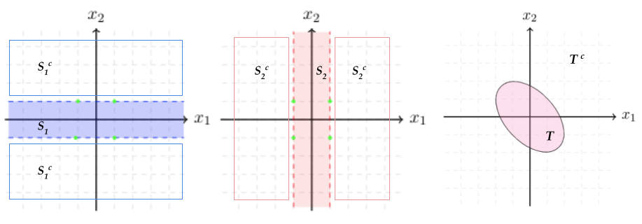
Figure 3: The mixture of partitions that corresponds to the Max-Cut problem. In figures $(a)$ and $(b)$, we partition the Euclidean space using fat hyperplanes (the blue set $S_{1}$ and the red set $S_{2}$ respectively) and their complements $S_{1}^{c}=\mathbb{R}^{d}\setminus S_{1}$ and $S_{2}^{c}=\mathbb{R}^{d}\setminus S_{2}$. The third figure $(c)$ partitions $\mathbb{R}^{d}$ using the ellipsoid $T=\{\bm{x}:\bm{x}^{T}\bm{\Sigma}^{-1}\bm{x}\leq q\}$ and its complement $T^{c}=\mathbb{R}^{d}\setminus T$ (for some $d\times d$ covariance matrix $\bm{\Sigma}$ and positive real $q$).

Fix the covariance matrix $\bm{\Sigma}=\bm{L}_{G}^{-1}\mathrm{opt}$ , i.e., $\bm{\Sigma}$ is the inverse of the Laplacian normalized by $\mathrm{opt}$. We let $T=\{\bm{x}:\bm{x}^{T}\bm{\Sigma}^{-1}\bm{x}\leq q\}$ for some positive value $q$ to be defined later (see Figure 2(b) and Figure 3(c)). Then, we let $\mathcal{T}=\{T,T^{c}\}$. We construct a mixture $\pi$ of these partitions by picking each one uniformly at random, i.e., with probability $1/(d+1)$.

Let us assume that there exists an algorithm that, given access to samples from $\mathcal{N}_{\pi}(\bm{\mu}^{\star},\bm{\Sigma})$, with known covariance $\bm{\Sigma}$, computes, in time $\mathrm{poly}(d)$, a mean vector $\bm{\mu}$ so that the output distributions are matched, i.e., $\mathrm{TV}(\mathcal{N}_{\pi}(\bm{\mu},\bm{\Sigma}),\mathcal{N}_{\pi}(\bm{\mu}^{\star},\bm{\Sigma}))$ is upper bounded by $1/d^{c}$ for some absolute constant $c>1$. Equivalently this means that the mass that $\mathcal{N}(\bm{\mu},\bm{\Sigma})$ assigns to each set $S_{i}$ and $T$ is within $\mathrm{poly}(1/d)$ of the corresponding mass that $\mathcal{N}_{\pi}(\bm{\mu}^{\star},\bm{\Sigma})$ assigns to the same set. There are two main challenges in order to prove the reduction:

1. How can we generate coarse samples from $\mathcal{N}_{\pi}(\bm{\mu}^{\star},\bm{\Sigma})$ since $\bm{\mu}^{\star}$ is the solution of the Max-Cut problem and therefore is unknown?

2. Given $\mathrm{opt}$, is it possible to pick the threshold $q$ of the ellipsoid $T=\{\bm{x}\in\mathbb{R}^{d}:\bm{x}^{T}\bm{\Sigma}^{-1}\bm{x}\leq q\}$ so that any vector $\bm{\mu}$ (rounded to belong in $\{-1,1\}^{d}$), that achieves $\mathcal{N}(\bm{\mu},\bm{\Sigma};T)\approx\mathcal{N}(\bm{\mu}^{\star},\bm{\Sigma};T)$ and $\mathcal{N}(\bm{\mu},\bm{\Sigma};S_{i})\approx\mathcal{N}(\bm{\mu}^{\star},\bm{\Sigma};S_{i})$, also achieves an approximation ratio better than $16/17$ for the Max-Cut objective ?

The key observation to answer the first question is that, by the rotation invariance of the Gaussian distribution, the probability $\mathcal{N}(\bm{\mu}^{\star},\bm{\Sigma};T)=\operatorname*{\mathbf{Pr}}_{\bm{x}\sim\mathcal{N}(\bm{\mu}^{\star},\bm{\Sigma})}\big{[}\bm{x}^{T}\bm{\Sigma}^{-1}\bm{x}\leq q\big{]}$ is a constant $p$ that only depends on the value $\mathrm{opt}$ of the Max-Cut problem. Therefore, having this value $p$, we can flip a coin with this probability and give the coarse sample $T$ if we get heads and $T^{c}$ otherwise. Similarly, the value of $\mathcal{N}(\bm{\mu}^{\star},\bm{\Sigma};S_{i})$ is an absolute constant that does not depend on $\bm{\mu}^{\star}\in\{-1,1\}^{d}$ and therefore we can again simulate coarse samples by flipping a coin with probability equal to $\mathcal{N}(\bm{\mu}^{\star},\bm{\Sigma};S_{i})$.

To resolve the second question, we first show that any vector $\bm{\mu}$ that approximately matches the probabilities of the $d$ fat halfspaces, lies very close to a corner of the hypercube, see Lemma 12. Therefore, by rounding this guess $\bm{\mu}$, we obtain exactly a corner of the hypercube without affecting the probability assigned to the ellipsoid constraint by a lot. We then show that any vector of the hypercube that almost matches the probability of the ellipsoid achieves large cut value. In particular, we prove that there exists a value for the threshold $q$ of the ellipsoid $\bm{x}^{T}\bm{\Sigma}^{-1}\bm{x}\leq q$ that makes the probability $\mathcal{N}(\bm{\mu},\bm{\Sigma};T)$ very sensitive to changes of $\bm{\mu}$. Therefore, the only way for the algorithm to match the observed probability is to find a $\bm{\mu}$ that achieves large cut value. We show the following lemma.

Lemma 10 (Sensitivity of Gaussian Probability of Ellipsoids).

Let $\mathcal{N}(\bm{\mu}^{\star},\bm{\Sigma})$, $\mathcal{N}(\bm{\mu},\bm{\Sigma})$ be $d$-dimensional Gaussian distributions. Let $\bm{v}^{\star}=\bm{\Sigma}^{-1/2}\bm{\mu}^{\star}$, $\bm{v}=\bm{\Sigma}^{-1/2}\bm{\mu}$ and assume that $\|\bm{v}\|_{2}\leq\|\bm{v}^{\star}\|_{2}=1$. Denote $q=d+\|\bm{v}^{\star}\|^{2}_{2}+\sqrt{2d+4\|\bm{v}^{\star}\|_{2}^{2}}$. Then, assuming $d$ is larger than some sufficiently large absolute constant, it holds that

$$\Big{|}\operatorname*{\mathbf{Pr}}_{\bm{x}\sim\mathcal{N}(\bm{\mu}^{\star},\bm{\Sigma})}\big{[}\bm{x}^{T}\bm{\Sigma}^{-1}\bm{x}\leq q\big{]}-\operatorname*{\mathbf{Pr}}_{\bm{x}\sim\mathcal{N}(\bm{\mu},\bm{\Sigma})}\big{[}\bm{x}^{T}\bm{\Sigma}^{-1}\bm{x}\leq q\big{]}\Big{|}\geq\frac{\|\bm{v}^{\star}\|_{2}^{2}-\|\bm{v}\|_{2}^{2}}{6\sqrt{2d+4}}-o(1/\sqrt{d})\,.$$

Notice that with $\bm{\Sigma}=\bm{L}_{G}^{-1}\mathrm{opt}$, in the above lemma, we have $\|\bm{v}^{\star}\|_{2}^{2}=1$, since $\bm{\mu}^{\star}$ achieves cut value $\mathrm{opt}$. By assumption, we know that the learning algorithm can find a guess $\bm{\mu}$ that makes the left hand side of the inequality of Lemma 10 smaller than $\mathrm{poly}(1/d)$. Thus, we obtain that, for $d$ large enough, it must be that $\|\bm{v}\|_{2}^{2}=\bm{\mu}^{T}\bm{L}_{G}\bm{\mu}/\mathrm{opt}\geq 16/17$. Therefore, $\bm{\mu}$ achieves value greater than $(16/17)\mathrm{opt}$.

Remark 3.

The transformation $\pi$ used in the above hardness result is not information preserving. In Theorem 5, we prove that it is computationally hard to find a vector $\bm{\mu}\in\mathbb{R}^{d}$ that matches in total variation the observed distribution over coarse labels. In contrast, as we will see in the upcoming Section 4.2, when the sets of the partitions are convex, we show that there is an efficient algorithm that can solve the same problem and compute some $\bm{\mu}\in\mathbb{R}^{d}$ such that $\mathrm{TV}(\mathcal{N}_{\pi}(\bm{\mu}^{\star}),\mathcal{N}_{\pi}(\bm{\mu}))$ is small regardless of whether the transformation $\pi$ is information preserving. When the transformation is information preserving, we can further show that the vector $\bm{\mu}$ that we compute will be close to $\bm{\mu}^{\star}$.

4.1.2 Sensitivity of Gaussian Probabilities

We now prove Lemma 10, namely that the probability of an ellipsoid with respect to the Gaussian distribution is sensitive to small changes of its mean.

Proof of Lemma 10.

We first observe that

$$\operatorname*{\mathbf{Pr}}_{\bm{x}\sim\mathcal{N}(\bm{\mu},\bm{\Sigma})}\big{[}\bm{x}^{T}\bm{\Sigma}^{-1}\bm{x}\leq q\big{]} =\operatorname*{\mathbf{Pr}}_{\bm{x}\sim\mathcal{N}(\bm{0},\bm{I})}\big{[}\bm{x}^{T}\bm{x}+2\bm{\mu}^{T}\bm{\Sigma}^{-1/2}\bm{x}\leq q-\bm{\mu}^{T}\bm{\Sigma}^{-1}\bm{\mu}\big{]}$$

$$=\operatorname*{\mathbf{Pr}}_{\bm{x}\sim\mathcal{N}(\bm{0},\bm{I})}\big{[}\bm{x}^{T}\bm{x}+2\bm{v}^{T}\bm{x}\leq q-\|\bm{v}\|_{2}^{2}\big{]},$$

where $\bm{v}=\bm{\Sigma}^{-1/2}\bm{\mu}$. Similarly, we have $\operatorname*{\mathbf{Pr}}_{\bm{x}\sim\mathcal{N}(\bm{\mu}^{\star},\bm{\Sigma})}\big{[}\bm{x}^{T}\bm{\Sigma}^{-1}\bm{x}\leq q\big{]}=\operatorname*{\mathbf{Pr}}_{\bm{x}\sim\mathcal{N}(\bm{0},\bm{I})}\big{[}\bm{x}^{T}\bm{x}+2(\bm{v}^{\star})^{T}\bm{x}\leq q-\|\bm{v}^{\star}\|_{2}^{2}\big{]},$ where $\bm{v}^{\star}=\bm{\Sigma}^{-1/2}\bm{\mu}^{\star}$. From the rotation invariance of the Gaussian distribution, we may assume, without loss of generality, that $\bm{v}=\|\bm{v}\|\bm{e}_{1}$ and $\bm{v}^{\star}=\|\bm{v}^{\star}\|\bm{e}_{1}$. Notice that $(\|\bm{v}\|_{2}+\bm{x}_{1})^{2}+\sum_{i=2}^{d}\bm{x}_{i}^{2}$ is a sum of independent random variables. To estimate these probabilities we are going to use the central limit theorem.

Lemma 11 (CLT, Theorem 1, Chapter XVI in [Fel57] ).

Let $X_{1},\ldots,X_{n}$ be independent random variables with $\operatorname*{\mathbf{E}}[|X_{i}|^{3}]<+\infty$ for all $i$. Let $m_{1}=\operatorname*{\mathbf{E}}[\sum_{i=1}^{n}X_{i}]$ and $m_{j}=\sum_{i=1}^{n}\operatorname*{\mathbf{E}}[(X_{i}-\operatorname*{\mathbf{E}}[X_{i}])^{j}]$. Then,

$$\operatorname*{\mathbf{Pr}}\left[\frac{(\sum_{i=1}^{n}X_{i})-m_{1}}{\sqrt{m_{2}}}\leq x\right]-\Phi(x)=m_{3}\frac{(1-x^{2})\phi(x)}{6m_{2}^{3/2}}+o\left(n/m_{2}^{3/2}\right)\,,$$

where $\Phi(\cdot)$, resp., $\phi(\cdot)$ is the CDF resp., PDF of the standard normal distribution and the convergence is uniform for all $x\in\mathbb{R}$.

Using the above central limit theorem we obtain

$$\operatorname*{\mathbf{Pr}}_{\bm{x}\sim\mathcal{N}(\bm{0},\bm{I})}\left[(\|\bm{v}^{\star}\|_{2}+\bm{x}_{1})^{2}+\sum_{i=2}^{d}\bm{x}_{i}^{2}\leq q\right]=\Phi(\bar{q}_{1})+O\left(\frac{1}{\sqrt{d}}\right)(1-\bar{q_{1}}^{2})\phi(\bar{q}_{1})+o\left(1/\sqrt{d}\right)\,,$$

where $\bar{q}_{1}=\frac{q-(d+\|\bm{v}^{\star}\|^{2}_{2})}{\sqrt{2d+4\|\bm{v}^{\star}\|^{2}_{2}}}$. Since $q=d+\|\bm{v}^{\star}\|^{2}+\sqrt{2d+4\|\bm{v}^{\star}\|^{2}_{2}}$ we obtain $\bar{q}_{1}=1$ and therefore

$$\operatorname*{\mathbf{Pr}}_{\bm{x}\sim\mathcal{N}(\bm{0},\bm{I})}\left[\bm{x}^{T}\bm{x}+2(\bm{v}^{\star})^{T}\bm{x}\leq q-\|\bm{v}^{\star}\|_{2}^{2}\right]=\Phi(1)+o\left(1/\sqrt{d}\right)\,.$$

Similarly, from the central limit theorem, we obtain

$$\operatorname*{\mathbf{Pr}}_{\bm{x}\sim\mathcal{N}(\bm{0},\bm{I})}\left[\left(\|\bm{v}\|_{2}+\bm{x}_{1}\right)^{2}+\sum_{i=2}^{d}\bm{x}_{i}^{2}\leq q\right]=\Phi(\bar{q}_{2})+O\left(\frac{1}{\sqrt{d}}\right)(1-\bar{q_{2}}^{2})\phi(\bar{q}_{2})+o\left(1/\sqrt{d}\right)\,,$$

where $\bar{q}_{2}=\frac{q-(d+\|\bm{v}\|^{2}_{2})}{\sqrt{2d+4\|\bm{v}\|^{2}_{2}}}=1+O(1/\sqrt{d})$. Therefore, we have

$$\operatorname*{\mathbf{Pr}}_{\bm{x}\sim\mathcal{N}(\bm{0},\bm{I})}\left[\bm{x}^{T}\bm{x}+2\bm{v}^{T}\bm{x}\leq q-\|\bm{v}\|_{2}^{2}\right]=\Phi(\bar{q}_{2})+o\left(1/\sqrt{d}\right)\,.$$

Moreover, we have that $\bar{q}_{2}\geq 1+(\|\bm{v}^{\star}\|_{2}^{2}-\|\bm{v}\|_{2}^{2})/(\sqrt{2d+4\|\bm{v}\|^{2}_{2}})$. Using the fact that $d$ is sufficiently large and standard approximation results on the Gaussian CDF, we obtain

$$\Phi\left(1+\frac{\|\bm{v}^{\star}\|_{2}^{2}-\|\bm{v}\|_{2}^{2}}{\sqrt{2d+4\|\bm{v}\|_{2}^{2}}}\right)-\Phi(1)\geq(\|\bm{v}^{\star}\|_{2}^{2}-\|\bm{v}\|_{2}^{2})/\left(6\sqrt{2d+4\|\bm{v}\|_{2}^{2}}\right)\,,$$

and, since $\|\bm{v}\|_{2}\leq 1$, we conclude that the left-hand side satisfies

$$\Phi\left(1+\frac{\|\bm{v}^{\star}\|_{2}^{2}-\|\bm{v}\|_{2}^{2}}{\sqrt{2d+4\|\bm{v}\|_{2}^{2}}}\right)-\Phi(1)\geq(\|\bm{v}^{\star}\|_{2}^{2}-\|\bm{v}\|_{2}^{2})/\left(6\sqrt{2d+4}\right)\,.$$

The result follows. ∎

We will also require the following sensitivity lemma about the Gaussian probability of bands, i.e., sets of the form $\{\bm{x}:|\bm{x}_{i}|\leq 1\}$. We show that the probabilities of such regions are also sensitive under perturbations of the mean of the Gaussian. This means that any vector $\bm{\mu}$ that has $\operatorname*{\mathbf{Pr}}_{\bm{x}\sim\mathcal{N}(\bm{\mu},\bm{\Sigma})}\big{[}-1\leq\bm{x}_{i}\leq 1\big{]}$ close to $\operatorname*{\mathbf{Pr}}_{\bm{x}\sim\mathcal{N}(\bm{\mu}^{\star},\bm{\Sigma})}\big{[}-1\leq\bm{x}_{i}\leq 1\big{]}$ must be very close to a corner of the hypercube.

Lemma 12 (Sensitivity of Gaussian Probability of Bands).

Let $\mathcal{N}(\bm{\mu}^{\star},\bm{\Sigma}),\mathcal{N}(\bm{\mu},\bm{\Sigma})$ be two $d$-dimensional Gaussian distributions with $\bm{e}_{i}^{T}\bm{\Sigma}\bm{e}_{i}\leq Q$, and $|\bm{\mu}_{i}^{\star}|=1$ for all $i\in[d]$. Then, for any $i\in[d]$, it holds that

$$\left|\operatorname*{\mathbf{Pr}}_{\bm{x}\sim\mathcal{N}(\bm{\mu}^{\star},\bm{\Sigma})}\big{[}-1\leq\bm{x}_{i}\leq 1\big{]}-\operatorname*{\mathbf{Pr}}_{\bm{x}\sim\mathcal{N}(\bm{\mu},\bm{\Sigma})}\big{[}-1\leq\bm{x}_{i}\leq 1\big{]}\right|\geq c\cdot\frac{\min(1,(1-|\bm{\mu}_{i}|)^{2})}{Q^{4}}\,,$$

for some absolute constant $c\in(0,1]$.

Proof.

Let us fix $i\in[d]$, define $\mu^{\star}$ (resp. $\mu$) for $\bm{\mu}^{\star}_{i}$ (resp. $\bm{\mu}_{i}$), and $\sigma^{2}=\bm{\Sigma}_{ii}$. Without loss of generality since both Gaussians have the same variance $\sigma$ by symmetry we may assume that $\mu^{\star}=1$ and $\mu\in[0,+\infty)$. We first deal with the case $\mu>1$. We have

$$\operatorname*{\mathbf{Pr}}_{\bm{x}\sim\mathcal{N}(\bm{\mu}^{\star},\bm{\Sigma})}\big{[}-1\leq\bm{x}_{i}\leq 1\big{]} -\operatorname*{\mathbf{Pr}}_{\bm{x}\sim\mathcal{N}(\bm{\mu},\bm{\Sigma})}\big{[}-1\leq\bm{x}_{i}\leq 1\big{]}$$

$$=\operatorname*{\mathbf{E}}_{t\sim\mathcal{N}(1,\sigma^{2})}\left[\bm{1}\{|t|\leq 1\}\left(1-\frac{\mathcal{N}(\mu,\sigma^{2};t)}{\mathcal{N}(1,\sigma^{2};t)}\right)\right]\,.$$

We have that since $\mu>1$ the ratio $\frac{\mathcal{N}(\mu,\sigma^{2};t)}{\mathcal{N}(1,\sigma^{2};t)}=e^{\frac{(\mu-1)(-\mu+2t-1)}{2\sigma^{2}}}$ is maximized for $t=1$ and has maximum value $e^{-\frac{(\mu-1)^{2}}{2\sigma^{2}}}$. By taking the derivative with respect to $\sigma$ we observe that the probability that $N(1,\sigma)$ assigns to $[-1,1]$ is decreasing with respect to $\sigma$ and therefore it is minimized for $\sigma=1$. We have that $\operatorname*{\mathbf{Pr}}_{t\sim\mathcal{N}(1,\sigma)}[-1<t<1]=\Omega(1/\sigma)$ and therefore $\operatorname*{\mathbf{Pr}}_{\bm{x}\sim\mathcal{N}(\bm{\mu}^{\star},\bm{\Sigma})}\big{[}-1\leq\bm{x}_{i}\leq 1\big{]}-\operatorname*{\mathbf{Pr}}_{\bm{x}\sim\mathcal{N}(\bm{\mu},\bm{\Sigma})}\big{[}-1\leq\bm{x}_{i}\leq 1\big{]}\geq C\cdot\left(1-e^{-\frac{(\mu-1)^{2}}{2\sigma^{2}}}\right).$ We can obtain the significantly weaker lower bound of $c\min(1,(1-|\mu|)^{2})$ for some absolute constant $c\in(0,1]$ by using the inequality $1-e^{-x}\geq 1/2\min(1,x)$ that holds for all $x\in[0,+\infty)$.

We now deal with the case $\mu\in[0,1)$. In that case the expression of their ratio of the densities of $\mathcal{N}(1,\sigma)$ and $\mathcal{N}(\mu,\sigma)$ derived above shows us that they cross at $t=(1+\mu)/2$. Therefore, they completely cancel out in the interval $[\mu,1]$. We have $\operatorname*{\mathbf{Pr}}_{\bm{x}\sim\mathcal{N}(\bm{\mu},\bm{\Sigma})}[-1\leq\bm{x}_{i}\leq 1]-\operatorname*{\mathbf{Pr}}_{\bm{x}\sim\mathcal{N}(\bm{\mu}^{\star},\bm{\Sigma})}[-1\leq\bm{x}_{i}\leq 1]=\operatorname*{\mathbf{Pr}}_{t\sim\mathcal{N}(\mu,\sigma)}[-1\leq t\leq\mu]-\operatorname*{\mathbf{Pr}}_{t\sim\mathcal{N}(1,\sigma)}[-1\leq t\leq\mu]=\Omega((1-\mu)/(1+\sigma^{4}))\,,$ where to obtain the last inequality we use standard approximations of Gaussian integrals. Combining the above two cases we obtain the claimed lower bound.

∎

4.1.3 The Proof of Theorem 5

We are now ready to provide the complete proof of Theorem 5. Consider an instance of Max-Cut with $|V|=d$ and optimal value $\mathrm{opt}=O(d^{2})$. Let $\bm{L}_{G}$ be the Laplacian matrix of the (connected) graph $G$. Since the minimum eigenvalue of $\bm{L}_{G}$ is $0$, we project the matrix onto the subspace $V$ that is orthogonal to $\bm{1}=(1,\ldots,1)$. We introduce a $(d-1)\times d$ partial isometry $\bm{R}$, that satisfies $\bm{R}\bm{R}^{T}=\bm{I}$ and $\bm{R}\bm{1}=\bm{0}$, i.e., $\bm{R}$ projects vectors to the subspace $V$. We consider $\bm{L}_{G}^{\prime}=\bm{R}\bm{L}_{G}\bm{R}^{T}$. It suffices to find a solution $\bm{x}\in V$ and then project back to $\mathbb{R}^{d}$: $\bm{y}=\bm{R}^{T}\bm{x}$. We note that the matrix $\bm{L}^{\prime}_{G}$ is positive definite (the smallest eigenvalue of $\bm{L}_{G}^{\prime}$ is equal to the second smallest eigenvalue of $\bm{L}_{G}$) and preserves the optimal score value, in the sense that

$$\mathrm{opt}=\max_{\bm{y}\in\mathbb{R}^{d}}\bm{y}^{T}\bm{L}_{G}\bm{y}=\max_{\bm{x}\in\mathbb{R}^{d}}(\bm{R}^{T}\bm{x})^{T}\bm{L}_{G}(\bm{R}^{T}\bm{x})=\max_{\bm{x}\in V}\bm{x}^{T}\bm{L}_{G}^{\prime}\bm{x}\,.$$

Assume that there exists an efficient black-box algorithm $\mathcal{A}$, that, given sample access to a generative process of coarse Gaussian data $\mathcal{N}_{\pi}(\bm{\mu}^{\star},\bm{\Sigma})$ with known covariance matrix $\bm{\Sigma}$, computes an estimate $\widetilde{\bm{\mu}}$ in $\mathrm{poly}(d)$ time, that satisfies

$$\mathrm{TV}(\mathcal{N}_{\pi}(\widetilde{\bm{\mu}},\bm{\Sigma}),\mathcal{N}_{\pi}(\bm{\mu}^{\star},\bm{\Sigma}))<1/d^{c}\,.$$

We choose the known covariance matrix to be equal to $\bm{\Sigma}=(\bm{L}_{G}^{\prime})^{-1}\mathrm{opt}$, where $\mathrm{opt}$ is the given optimal Max-Cut value and let $\bm{\mu}^{\star}\in\{-1,1\}^{d-1}$ be the unknown mean vector. Recall that, not only the black-box algorithm $\mathcal{A}$, but also the generative process that we design is agnostic to the true mean. However, as we will see the knowledge of the optimal value $\mathrm{opt}$ and the fact that the true mean lies in the hypercube $\{-1,1\}^{d-1}$ suffice to generate samples from the true coarse generative process $\mathcal{N}_{\pi}(\bm{\mu}^{\star},\bm{\Sigma})$.

In what follows, we will construct such a coarse generative process using the objective function and the constraints of the Max-Cut problem. Specifically, we will design a collection $\mathcal{B}=\{\mathcal{S}_{1},\dots,\mathcal{S}_{d-1},\mathcal{T}\}$ of $d$ partitions of the $d$-dimensional Euclidean space and let the partition distribution $\pi$ be the uniform probability measure over $\mathcal{B}$.

We define the partitions as follows: for any $i=1,\dots,d-1$, let $S_{i}=\{\bm{x}:-1\leq\bm{x}_{i}\leq 1\}$ and $\mathcal{S}_{i}=\{S_{i},S_{i}^{c}\}$. These $d-1$ partitions simulate the integrality constraints of Max-Cut , i.e., the solution vector should lie in the hypercube $\{-1,1\}^{d-1}$. It remains to construct $\mathcal{T}$, which corresponds to the quadratic objective of $\textsc{Max-Cut }.$ We let $T=\{\bm{x}\in\mathbb{R}^{d}:\bm{x}^{T}\bm{\Sigma}^{-1}\bm{x}\leq q\}$, for $q>0$ to be decided. Then, we let $\mathcal{T}=\{T,T^{c}\}$. Recall that the known covariance matrix $\bm{\Sigma}=(\bm{L}_{G}^{\prime})^{-1}\mathrm{opt}$ lies in $\mathbb{R}^{(d-1)\times(d-1)}$ and, so, we will use $d-1$ bands (i.e., fat hyperplanes).

The main question to resolve is how to generate efficiently samples from the designed general partition, i.e., the distribution $\mathcal{N}_{\pi}(\bm{\mu}^{\star},\bm{\Sigma})$, without knowing the value of $\bm{\mu}^{\star}$. The key observation is that, by the rotation invariance of the Gaussian distribution, the probability $\mathcal{N}(\bm{\mu}^{\star},\bm{\Sigma};T)=\operatorname*{\mathbf{Pr}}_{\bm{x}\sim\mathcal{N}(\bm{\mu}^{\star},\bm{\Sigma})}\big{[}\bm{x}^{T}\bm{\Sigma}^{-1}\bm{x}\leq q\big{]}$ is a constant $p$ that only depends on the value $\mathrm{opt}$ of the maximum cut (see the proof of Lemma 10). Therefore, having this value $p$, we can flip a coin with this probability and give the coarse sample $T$ if we get heads and $T^{c}$ otherwise. At the same time, the value of $\mathcal{N}(\bm{\mu}^{\star},\bm{\Sigma};S_{i})$ is an absolute constant that does not depend on $\bm{\mu}^{\star}\in\{-1,1\}^{d-1}$ and, therefore, we can again simulate coarse samples by flipping a coin with probability equal to $\mathcal{N}(\bm{\mu}^{\star},\bm{\Sigma};S_{i})$. More precisely, since $S_{i}$ is a symmetric interval around $0$, we have that

$$\operatorname*{\mathbf{Pr}}_{\bm{x}\sim\mathcal{N}(\bm{\mu}^{\star},\bm{\Sigma})}\big{[}-1\leq\bm{x}_{i}\leq 1]=\operatorname*{\mathbf{Pr}}_{t\sim\mathcal{N}(1,\bm{\Sigma}_{ii})}\big{[}-1\leq t\leq 1]\,.$$

Notice that the above constant only depends on the known constant $\bm{\Sigma}_{ii}$ and can be computed to very high accuracy using well known approximations of the Gaussian integral or rejection sampling. Moreover, all the probabilities $\mathcal{N}(\bm{\mu}^{\star},\bm{\Sigma};S_{i}),\mathcal{N}(\bm{\mu}^{\star},\bm{\Sigma};T)$ are at least polynomially small in $1/d$. In particular, $\mathcal{N}(\bm{\mu}^{\star},\bm{\Sigma};S_{i})$, is always larger than $\Omega(1/\sigma)\geq\mathrm{poly}(1/d)$ and smaller than $1/2$ and $\mathcal{N}(\bm{\mu}^{\star},\bm{\Sigma};T)=\Phi(1)+o(1/\sqrt{d})$ , see the proof of Lemma 10. Having these values we can generate samples from $\mathcal{N}_{\pi}$ as follows:

1. Pick one of the $d$ sets $S_{1},\ldots,S_{d-1},T$ uniformly at random.

2. Flip a coin with success probability equal to the probability of the corresponding sets and return either the set or its complement.

Giving sample access to the designed oracle with $\mathcal{B}=\{\mathcal{S}_{1},\dots,\mathcal{S}_{d-1},\mathcal{T}\}$, the black-box algorithm $\mathcal{A}$ computes efficiently and returns an estimate $\widetilde{\bm{\mu}}\in\mathbb{R}^{d-1}$, that satisfies

$$\mathrm{TV}(\mathcal{N}_{\pi}(\widetilde{\bm{\mu}},\bm{\Sigma}),\mathcal{N}_{\pi}(\bm{\mu}^{\star},\bm{\Sigma}))<o(1/d^{c})\,.$$

We proceed with two claims: $(i)$ the algorithm’s output $\widetilde{\bm{\mu}}$ should lie in a ball of radius $\mathrm{poly}(1/d)$, centered at one of the vertices of the hypercube $\{-1,1\}^{d-1}$ and $(ii)$ it will hold that the rounded vector $\widehat{\bm{\mu}}=(\mathrm{sgn}(\widetilde{\bm{\mu}}_{i}))_{1\leq i\leq d-1}\in\{-1,1\}^{d-1}$ will attain a cut score, that approximates the Max-Cut within a factor larger than $16/17$. By the algorithm’s guarantee, since $\pi$ is the uniform distribution, we get that

$$|\mathcal{N}(\widetilde{\bm{\mu}},\bm{\Sigma};T)-\mathcal{N}(\bm{\mu}^{\star},\bm{\Sigma};T)|+\sum_{i=1}^{d-1}|\mathcal{N}(\widetilde{\bm{\mu}},\bm{\Sigma};S_{i})-\mathcal{N}(\bm{\mu}^{\star},\bm{\Sigma};S_{i})|=o(1/d^{c-1})\,.$$

Hence, we get that each of the above $d$ summands is at most $o(1/d^{c-1})$.

Claim 4.

It holds that $\|\widetilde{\bm{\mu}}-\widehat{\bm{\mu}}\|_{\infty}<\epsilon$, where $\widetilde{\bm{\mu}}$ is the black-box algorithm’s estimate and $\widehat{\bm{\mu}}$ its rounding to $\{-1,1\}^{d-1}$.

Proof.

For any coordinate $i\in[d-1],$ we will apply Lemma 12 in order to bound the distance between the estimated guess and the true, based on the Gaussian mass gap in each one of the $d-1$ bands.

Note that $|\bm{\mu}^{\star}_{i}|=1$ for all $i\in[d-1]$. Also, note that the $(d-1)\times(d-1)$ matrix $\bm{L}_{G}^{\prime}$ is positive definite and the minimum eigenvalue $\lambda(\bm{L}_{G}^{\prime})$ is equal to the second smallest eigenvalue of the $d\times d$ Laplacian matrix $\bm{L}_{G}$. It holds that $\lambda(\bm{L}_{G}^{\prime})>0.$ Hence, the maximum entry of the covariance matrix $\bm{\Sigma}=(\bm{L}_{G}^{\prime})^{-1}\mathrm{opt}$ is upper bounded by $1/(\mathrm{opt}\cdot\lambda(\bm{L}_{G}^{\prime}))<Q=\mathrm{poly}(d)$ for some value $Q$. Using Lemma 12 and the algorithm’s guarantee, we have that

$$(|\widetilde{\bm{\mu}}_{i}|-1)^{2}/Q^{4}\leq|\mathcal{N}(\widetilde{\bm{\mu}},\bm{\Sigma};S_{i})-\mathcal{N}(\bm{\mu}^{\star},\bm{\Sigma};S_{i})|=o\left(1/d^{c-1}\right)\,.$$

For sufficiently large $c$, we get that each coordinate of the estimated vector $\widetilde{\bm{\mu}}$ lies in an interval, centered at either $1$ or $-1$ of length $o(1/d^{c-1})$. This implies that $\|\widetilde{\bm{\mu}}-\bm{w}\|_{\infty}<\epsilon$ for some $\epsilon=o(1/d^{c-1})$ and some vertex $\bm{w}$ of the hypercube $\{-1,1\}^{d-1}$. Hence, we have that $\widetilde{\bm{\mu}}$ should lie in a ball, with respect to the $L_{\infty}$ norm, centered at one of the vertices of the $(d-1)$-hypercube with radius of order $\epsilon$ and note that this vertex corresponds to the rounded vector $\widehat{\bm{\mu}}$ of the estimated vector. ∎

We continue by claiming that the rounded vector $\widehat{\bm{\mu}}$ attains a Max-Cut value, that approximates the optimal value $\mathrm{opt}$ withing a factor strictly larger than $16/17$.

Claim 5.

The Max-Cut value of the rounded vector $\widehat{\bm{\mu}}\in\{-1,1\}^{d-1}$ satisfies

$$\widehat{\bm{\mu}}^{T}\bm{L}_{G}^{\prime}\widehat{\bm{\mu}}>(16/17)\cdot\mathrm{opt}\,.$$

Proof.

We will make use of Lemma 10, in order to get the desired result via the Gaussian mass gap between the two means on the designed ellipsoid. In order to apply this Lemma, note that, for the true mean $\bm{\mu}^{\star}$, we have that $\|\bm{v}^{\star}\|_{2}^{2}=\|(\bm{\Sigma}^{\star})^{-1/2}\bm{\mu}^{\star}\|_{2}^{2}=((\bm{\mu}^{\star})^{T}\bm{L}_{G}^{\prime}\bm{\mu}^{\star})/\mathrm{opt}=1$, since the true mean attains the optimal Max-Cut score. Similarly, for the rounded estimated mean $\widehat{\bm{\mu}}$, the associated vector $\widehat{\bm{v}}$ satisfies $\|\widehat{\bm{v}}\|_{2}\leq 1$, since its cut value is at most $\mathrm{opt}$. So, we can apply Lemma 10 with $\bm{v}^{\star}=\bm{\Sigma}^{-1/2}\bm{\mu}^{\star}$ and $\bm{v}=\bm{\Sigma}^{-1/2}\widehat{\bm{\mu}}$ and get that

$$\frac{1-\left(\widehat{\bm{\mu}}^{T}\bm{L}_{G}^{\prime}\widehat{\bm{\mu}}\right)/\mathrm{opt}}{6\sqrt{2d+4}}-o\left(1/\sqrt{d}\right)<o\left(1/d^{c-1}\right)\,,$$

which implies that, for some small constant $c^{\prime}$, the value of the estimated mean satisfies $\widehat{\bm{\mu}}^{T}\bm{L}_{G}^{\prime}\widehat{\bm{\mu}}>(1-c^{\prime}-1/d^{c-1})\mathrm{opt}$. This implies that the algorithm $\mathcal{A}$ can approximate the Max-Cut value within a factor higher than $16/17$. ∎

Known Covariance vs. Identity Covariance.

Recall that our hardness result (Theorem 5) states that there is no algorithm with sample access to $\mathcal{N}_{\pi}({\bm{\mu}}^{\star})=\mathcal{N}_{\pi}({\bm{\mu}}^{\star},\bm{I}),$ that can compute a mean $\widetilde{\bm{\mu}}\in\mathbb{R}^{d}$ in $\mathrm{poly}(d)$ time such that $\mathrm{TV}(\mathcal{N}_{\pi}(\widetilde{\bm{\mu}}),\mathcal{N}_{\pi}(\bm{\mu}^{\star}))<1/d^{c}$ for some absolute constant $c>1$. In order to prove our hardness result, we assume that there exists such a black-box algorithm $\mathcal{A}$. Hence, to make use of $\mathcal{A}$, one should provide samples generated by a coarse Gaussian with identity covariance matrix. However, in our reduction, we show that we can generate samples from a coarse Gaussian (which is associated with the Max-Cut instance) that has known covariance matrix $\bm{\Sigma}$. Let us consider a sample $S\sim\mathcal{N}_{\pi}(\bm{\mu}^{\star},\bm{\Sigma})$. Since $\bm{\Sigma}$ is known, we can rotate the sets and give as input to the algorithm $\mathcal{A}$ the set

$$\bm{\Sigma}^{-1/2}\cdot S:=\left\{\bm{\Sigma}^{-1/2}\bm{x}:\bm{x}\in S\right\}\,,$$

i.e., we can implement the membership oracle $\mathcal{O}_{\bm{\Sigma}^{-1/2}\cdot S}(\cdot),$ assuming oracle access to $\mathcal{O}_{S}(\cdot)$. We have that $\mathcal{O}_{\bm{\Sigma}^{-1/2}\cdot S}(\bm{x})=\mathcal{O}_{S}(\bm{\Sigma}^{1/2}\bm{x})$. We continue with a couple of observations.

1. We first observe that, for any partition $\mathcal{S}$ of the $d$-dimensional Euclidean space, there exists another partition $\bm{\Sigma}^{-1/2}\cdot\mathcal{S}$ consisting of the sets $\bm{\Sigma}^{-1/2}\cdot S$, where $S\in\mathcal{S}$. Note that since $\bm{\Sigma}^{-1/2}$ is full rank, the mapping $\bm{x}\mapsto\bm{\Sigma}^{-1/2}\bm{x}$ is a bijection and so $\bm{\Sigma}^{-1/2}\cdot\mathcal{S}$ is a partition of the space with $\pi(\bm{\Sigma}^{-1/2}\cdot\mathcal{S})=\pi(\mathcal{S})$.

2. We have that $\bm{x}\in S$ if and only if $\bm{\Sigma}^{-1/2}\bm{x}\in\bm{\Sigma}^{-1/2}\cdot S$ and so

   $$\operatorname*{\mathbf{E}}_{\bm{x}\sim\mathcal{N}(\bm{\mu},\bm{\Sigma})}[\bm{1}\{\bm{x}\in S\}]=\operatorname*{\mathbf{E}}_{\bm{x}\sim\mathcal{N}(\bm{\mu},\bm{\Sigma})}[\bm{1}\{\bm{\Sigma}^{-1/2}\bm{x}\in\bm{\Sigma}^{-1/2}\cdot S\}]\,.$$

   Since it holds that $\bm{w}\sim\mathcal{N}(\bm{\mu},\bm{\Sigma})$ if and only if $\bm{w}=\bm{\Sigma}^{1/2}\bm{z}+\bm{\mu}$ with $\bm{z}\sim\mathcal{N}(\bm{0},\bm{I})$, we get for an arbitrary subset $S\subseteq\mathbb{R}^{d}$ that

   $$\operatorname*{\mathbf{E}}_{\bm{x}\sim\mathcal{N}(\bm{\mu},\bm{\Sigma})}[\bm{1}\{\bm{x}\in S\}] =\operatorname*{\mathbf{E}}_{\bm{x}\sim\mathcal{N}(\bm{0},\bm{I})}\left[\bm{1}\left\{\bm{\Sigma}^{-1/2}\left(\bm{\Sigma}^{1/2}\bm{x}+\bm{\mu}\right)\in\bm{\Sigma}^{-1/2}\cdot S\right\}\right]$$

   $$=\operatorname*{\mathbf{E}}_{\bm{x}\sim\mathcal{N}(\bm{\Sigma}^{-1/2}\bm{\mu},\bm{I})}\left[\bm{1}\{\bm{x}\in\bm{\Sigma}^{-1/2}\cdot S\}\right]\,.$$

Let us consider a set $S\subseteq\mathbb{R}^{d}$ distributed as $\mathcal{N}_{\pi}(\bm{\mu}^{\star},\bm{\Sigma}).$ This set is the one that the algorithm with the known covariance matrix works with. We are now ready to combine the above two observations in order to understand what is the input to the identity covariance matrix algorithm. We have that

$$\begin{split}\operatorname*{\mathbf{Pr}}_{S\sim\mathcal{N}_{\pi}(\bm{\mu}^{\star},\bm{\Sigma})}[S]&=\sum_{\mathcal{S}}\bm{1}\{S\in\mathcal{S}\}\pi(\mathcal{S})\mathcal{N}(\bm{\mu}^{\star},\bm{\Sigma};S)\\ &=\sum_{\mathcal{S}}\bm{1}\{S\in\mathcal{S}\}\pi(\mathcal{S})\mathcal{N}(\bm{\Sigma}^{-1/2}\bm{\mu}^{\star},\bm{I};\bm{\Sigma}^{-1/2}\cdot S)\\ &=\sum_{\bm{\Sigma}^{-1/2}\cdot\mathcal{S}}\bm{1}\{\bm{\Sigma}^{-1/2}\cdot S\in\bm{\Sigma}^{-1/2}\cdot\mathcal{S}\}\pi(\bm{\Sigma}^{-1/2}\cdot\mathcal{S})\mathcal{N}(\bm{\Sigma}^{-1/2}\bm{\mu}^{\star},\bm{I};\bm{\Sigma}^{-1/2}\cdot S)\\ &=\operatorname*{\mathbf{Pr}}_{S^{\prime}\sim\mathcal{N}_{\pi^{\prime}}(\bm{\Sigma}^{-1/2}\bm{\mu}^{\star},\bm{I})}[S^{\prime}]\,,\end{split}$$

where the set $S^{\prime}$ is distributed as $\mathcal{N}_{\pi^{\prime}}(\bm{\Sigma}^{-1/2}\bm{\mu}^{\star},\bm{I})$ where $\pi^{\prime}$ is the ’rotated’ partition distribution supported on the rotated partitions $\bm{\Sigma}^{-1/2}\cdot\mathcal{S}$ for each $\mathcal{S}$ with $\pi(\mathcal{S})>0$. We remark that the second equation follows from the second observation and the third equation from the first one. Hence, the algorithm $\mathcal{A}$ (the one that works with identity matrix) obtains the rotated sets (i.e., membership oracles) $\bm{\Sigma}^{-1/2}\cdot S$ and the (unknown) target mean vector is $\bm{u}=\bm{\Sigma}^{-1/2}\bm{\mu}^{\star}$.

4.2 Efficient Mean Estimation under Convex Partitions

In this section, we formally state and prove 2, which is stated in Section 1: we provide an efficient algorithm for Gaussian mean estimation under convex partitions. The following definition of information preservation is very similar with the one given in the introduction, see Definition 2. The difference is that we only require from $\pi$ to preserve the distances of Gaussians around the true Gaussian $\mathcal{N}(\bm{\mu}^{\star})$ as opposed to the distance of any pair of Gaussians $\mathcal{N}(\bm{\mu}^{\star})$: this is a somewhat more flexible assumption about the partition distribution $\pi$ and the true Gaussian $\mathcal{N}(\bm{\mu}^{*})$ as a pair.

Definition 13 (Information Preserving Partition Distribution for Gaussians).

Let $\alpha\in[0,1]$ and consider a $d$-dimensional Gaussian distribution $\mathcal{N}(\bm{\mu}^{\star})$. We say that $\pi$ is an $\alpha$-information preserving partition distribution with respect to the true Gaussian $\mathcal{N}(\bm{\mu}^{\star})$ if for any Gaussian distribution $\mathcal{N}(\bm{\mu})$, it holds that $\mathrm{TV}(\mathcal{N}_{\pi}(\bm{\mu}),\mathcal{N}_{\pi}(\bm{\mu}^{\star}))\geq\alpha\cdot\mathrm{TV}(\mathcal{N}(\bm{\mu}),\mathcal{N}(\bm{\mu}^{\star}))$.

We refer to Appendix C for a geometric condition, under which a partition is $\alpha$-information preserving. In particular, we prove that a partition is $\alpha$-information preserving if, for any hyperplane, it holds that the mass of the cells of the partition that do not intersect with the hyperplane is at least $\alpha$. This is true for most natural partitions, see e.g., the Voronoi diagram of Figure 1.

We continue with a formal statement of 2.

Theorem 14 (Gaussian Mean Estimation with Convex Partitions).

Let $\epsilon,\delta\in(0,1)$. Consider the generative process of coarse $d$-dimensional Gaussian data $\mathcal{N}_{\pi}(\bm{\mu}^{\star})$, as in Definition 4. Assume that the partition distribution $\pi$ is $\alpha$-information preserving and is supported on convex partitions of $\mathbb{R}^{d}$. The following hold.

1. The empirical log-likelihood objective

   $$\mathcal{L}_{N}(\bm{\mu})=\frac{1}{N}\sum_{i=1}^{N}\log\mathcal{N}(\bm{\mu};S_{i})$$

   is concave with respect to $\bm{\mu}$ where the sets $S_{i}$ for $i\in[N]$ are i.i.d. samples from $\mathcal{N}_{\pi}(\bm{\mu}^{\star})$.

2. There exists an algorithm, that draws $N=\widetilde{O}(d/(\epsilon^{2}\alpha^{2})\log(1/\delta))$ samples from $\mathcal{N}_{\pi}(\bm{\mu}^{\star})$ and computes an estimate $\widetilde{\bm{\mu}}$ that satisfies $\mathrm{TV}(\mathcal{N}(\widetilde{\bm{\mu}}),\mathcal{N}(\bm{\mu}^{\star}))\leq\epsilon\,,$ with probability at least $1-\delta$.

In this section, we discuss and establish the two structural lemmata required in order to prove Theorem 14. Our goal is to maximize the empirical log-likelihood objective

$$\mathcal{L}_{N}(\bm{\mu})=\frac{1}{N}\sum_{i=1}^{N}\log\mathcal{N}(\bm{\mu};S_{i})\,,$$ (4.1)

where the $N$ (convex) sets $S_{1},\ldots,S_{N}$ are drawn from the coarse Gaussian generative process $\mathcal{N}_{\pi}(\bm{\mu}^{\star})$. We first show that the above empirical likelihood is a concave objective with respect to $\bm{\mu}\in\mathbb{R}^{d}$. In the following lemma, we show that the log-probability of a convex set $S$, i.e., the function $\log\mathcal{N}(\bm{\mu};S)$ is a concave function of the mean $\bm{\mu}$.

Lemma 15 (Concavity of Log-Likelihood).

Let $S\subseteq\mathbb{R}^{d}$ be a convex set. The function $\log\mathcal{N}(\bm{\mu};S)$ is concave with respect to the mean vector $\bm{\mu}\in\mathbb{R}^{d}$.

In order to prove that the Hessian matrix of this objective is negative semi-definite, we use a variant of the Brascamp-Lieb inequality. Having established the concavity of the empirical log-likelihood, we next have to bound the sample complexity of the empirical log-likelihood. We prove the following lemma.

Lemma 16 (Sample Complexity of Empirical Log-Likelihood).

Let $\epsilon,\delta\in(0,1)$ and consider a generative process for coarse $d$-dimensional Gaussian data $\mathcal{N}_{\pi}(\bm{\mu}^{\star})$ (see Definition 4). Also, assume that every $\mathcal{S}\in\mathrm{supp}(\pi)$ is a convex partition of the Euclidean space. Let $N=\widetilde{\Omega}({d}/(\epsilon^{2}\alpha^{2})\log(1/\delta))$. Consider the empirical log-likelihood objective

$$\mathcal{L}_{N}(\bm{\mu})=\frac{1}{N}\sum_{i=1}^{N}\log\mathcal{N}(\bm{\mu};S_{i})\,.$$

Then, with probability at least $1-\delta$, we have that, for any Gaussian distribution $\mathcal{N}(\bm{\mu})$ that satisfies $\mathrm{TV}(\mathcal{N}(\bm{\mu}),\mathcal{N}(\bm{\mu}^{\star}))\geq\epsilon$, it holds that $\max_{\widetilde{\bm{\mu}}\in\mathbb{R}^{d}}\mathcal{L}_{N}(\widetilde{\bm{\mu}})-\mathcal{L}_{N}(\bm{\mu})\geq\Omega(\epsilon^{2}\alpha^{2})\,.$

The above lemma states that, given roughly $\widetilde{O}({d}/(\epsilon^{2}\alpha^{2}))$ samples from $\mathcal{N}_{\pi}(\bm{\mu}^{\star})$, we can guarantee that the maximizer $\widetilde{\bm{\mu}}$ of the empirical log-likelihood achieves a total variation gap at most $\epsilon$ against the true mean vector $\bm{\mu}^{\star},$ i.e., $\mathrm{TV}(\mathcal{N}(\widetilde{\bm{\mu}}),\mathcal{N}(\bm{\mu}^{\star}))\leq\epsilon$. In fact, thanks to the concavity of the empirical log-likelihood objective, it suffices to show that Gaussian distributions $\mathcal{N}(\bm{\mu})$, that satisfy $\mathrm{TV}(\mathcal{N}(\bm{\mu}),\mathcal{N}(\bm{\mu}^{\star}))>\epsilon$, will also be significantly sub-optimal solutions of the empirical log-likelihood maximization. The key idea in order to attain the desired sample complexity, is that is suffices to focus on guess vectors $\bm{\mu}$ that lie in a sphere of radius $\Omega(\epsilon)$. Technically, the proof of Lemma 16 relies on a concentration result of likelihood ratios and in the observation that, while the empirical log-likelihood objective $\mathcal{L}_{N}$ is concave (under convex partitions), the regularized objective $\mathcal{L}_{N}(\bm{\mu})+\|\bm{\mu}\|_{2}^{2}$ is convex with respect to the guess mean vector $\bm{\mu}$.

4.2.1 Concavity of Log-likelihood: Proof of Lemma 15

In this section, we show that the log-likelihood is concave when the underlying partitions are convex. The Hessian of the log-likelihood $\mathcal{L}$ for the set $S$ has a notable property. When restricted to a direction $\bm{v}\in\mathbb{R}^{d}$, the quadratic $\bm{v}^{T}(\nabla^{2}\mathcal{L})\bm{v}$ quantifies the variance reduction, observed between the distributions $\mathcal{N}_{S}$ (Gaussian conditioned on $S$) and $\mathcal{N}$ (unrestricted Gaussian, i.e., $S=\mathbb{R}^{d}$). When the set $S$ is convex (and, hence the indicator function $\bm{1}_{S}$ is log-concave), the variance of the unrestricted Gaussian is always larger than the conditional one. This intriguing result is an application of a variation of the Brascamp-Lieb inequality, due to Hargé (see Lemma 17 for the inequality that we utilize). Recall that, both the empirical and the population log-likelihood objectives are convex combinations of the function $f(\bm{\mu},\bm{\Sigma};S)=\log\mathcal{N}(\bm{\mu},\bm{\Sigma};S)$ and, hence, it suffices to show that $f$ is concave with respect to $\bm{\mu}\in\mathbb{R}^{d}$, when the set $S$ is convex.

Proof of Lemma 15.

Without loss of generality, we can take $\bm{\Sigma}=\bm{I}\in\mathbb{R}^{d\times d}$. Let $f(\bm{\mu};S)=\log\mathcal{N}(\bm{\mu},\bm{I};S)$ for an arbitrary convex set $S\subseteq\mathbb{R}^{d}$. The gradient $\nabla_{\bm{\mu}}f(\bm{\mu})$ of $f$ with respect to $\bm{\mu}$ is equal to

$$\nabla_{\bm{\mu}}\left(\log\int_{S}\frac{1}{\sqrt{(2\pi)^{d}}}\exp\left(-\frac{(\bm{x}-\bm{\mu})^{T}(\bm{x}-\bm{\mu})}{2}\right)d\bm{x}\right)=\frac{\int_{S}\bm{x}\exp(-(\bm{x}-\bm{\mu})^{T}(\bm{x}-\bm{\mu})/2)d\bm{x}}{\int_{S}\exp(-(\bm{x}-\bm{\mu})^{T}(\bm{x}-\bm{\mu})/2)d\bm{x}}-\bm{\mu}\,.$$

Hence, we get that

$$\nabla_{\bm{\mu}}f(\bm{\mu})=\operatorname*{\mathbf{E}}_{\bm{x}\sim\mathcal{N}_{S}(\bm{\mu},\bm{I})}[\bm{x}]-\bm{\mu}\,.$$

We continue with the computation of the Hessian of the function $f$ with respect to $\bm{\mu}$

$$\nabla_{\bm{\mu}}^{2}f(\bm{\mu})=-\bm{I}+\frac{\int_{S}\bm{x}(\bm{x}-\bm{\mu})^{T}\mathcal{N}(\bm{\mu},\bm{I};\bm{x})d\bm{x}}{\mathcal{N}(\bm{\mu},\bm{I};S)}-\frac{\Big{(}\int_{S}\bm{x}\mathcal{N}(\bm{\mu},\bm{I};\bm{x})d\bm{x}\Big{)}\Big{(}\int_{S}(\bm{x}-\bm{\mu})^{T}\mathcal{N}(\bm{\mu},\bm{I};\bm{x})d\bm{x}\Big{)}}{\mathcal{N}(\bm{\mu},\bm{I};S)^{2}}\,,$$

and, so, we have that

$$\nabla_{\bm{\mu}}^{2}f(\bm{\mu})=-\bm{I}+\Big{(}\operatorname*{\mathbf{E}}_{\bm{x}\sim\mathcal{N}_{S}(\bm{\mu},\bm{I})}[\bm{x}\bm{x}^{T}]-\operatorname*{\mathbf{E}}_{\bm{x}\sim\mathcal{N}_{S}(\bm{\mu},\bm{I})}[\bm{x}]\operatorname*{\mathbf{E}}_{\bm{x}\sim\mathcal{N}_{S}(\bm{\mu},\bm{I})}[\bm{x}^{T}]\Big{)}=\mathop{\mathbf{Cov}}_{\bm{x}\sim\mathcal{N}_{S}(\bm{\mu},\bm{I})}[\bm{x}]-\bm{I}\,.$$

Observe that, when $S=\mathbb{R}^{d}$, we get that both the gradient and the Hessian vanish. In order to show the concavity of $f$ with respect to the mean vector $\bm{\mu},$ consider an arbitrary vector $\bm{v}\in\mathbb{R}^{d}$ in the ball $\|\bm{v}\|_{2}=1$. We have the quadratic form

$$\bm{v}^{T}\nabla_{\bm{\mu}}^{2}f(\bm{\mu})\bm{v}=\bm{v}^{T}\mathop{\mathbf{Cov}}_{\bm{x}\sim\mathcal{N}_{S}(\bm{\mu},\bm{I})}[\bm{x}]\bm{v}-1=\operatorname*{\mathbf{E}}_{\bm{x}\sim\mathcal{N}_{S}(\bm{\mu},\bm{I})}\Big{[}\bm{(}\bm{v}^{T}\bm{x})^{2}\Big{]}-\Big{(}\operatorname*{\mathbf{E}}_{\bm{x}\sim\mathcal{N}_{S}(\bm{\mu},\bm{I})}[\bm{v}^{T}\bm{x}]\Big{)}^{2}-1\,.$$

In order to show the desired inequality, we will apply the following variant of the Brascamp-Lieb inequality.

Lemma 17 (Brascamp-Lieb Inequality, Hargé (see [Gui09])).

Let $g$ be convex function on $\mathbb{R}^{d}$ and let $S$ be a convex set on $\mathbb{R}^{d}$. Let $\mathcal{N}(\bm{\mu},\bm{\Sigma})$ be the Gaussian distribution on $\mathbb{R}^{d}$. It holds that

$$\operatorname*{\mathbf{E}}_{\bm{x}\sim N_{S}}\left[g\left(\bm{x}+\bm{\mu}-\operatorname*{\mathbf{E}}_{\bm{x}\sim\mathcal{N}_{S}}[\bm{x}]\right)\right]\leq\operatorname*{\mathbf{E}}_{\bm{x}\sim\mathcal{N}}[g(\bm{x})]\,.$$ (4.2)

We apply the above Lemma with $g(\bm{x})=(\bm{v}^{T}\bm{x})^{2}$. We get that

$$\int_{\mathbb{R}^{d}}(\bm{v}^{T}(\bm{x}+\bm{\mu}-\operatorname*{\mathbf{E}}_{y\sim\mathcal{N}_{S}(\bm{\mu},\bm{I})}\bm{y}))^{2}\cdot\frac{\bm{1}_{S}(\bm{x})\mathcal{N}(\bm{\mu},\bm{I};\bm{x})d\bm{x}}{\int_{\mathbb{R}^{d}}\bm{1}_{S}(\bm{x})\mathcal{N}(\bm{\mu},\bm{I};\bm{x})d\bm{x}}\leq\int_{\mathbb{R}^{d}}(\bm{v}^{T}\bm{x})^{2}\mathcal{N}(\bm{\mu},\bm{I};\bm{x})d\bm{x}\,.$$

Hence, we get the desired variance reduction in the direction $\bm{v}$

$$\operatorname*{\mathbf{V}}_{\bm{x}\sim\mathcal{N}_{S}(\bm{\mu},\bm{I})}[\bm{v}^{T}\bm{x}]\leq\operatorname*{\mathbf{V}}_{\bm{x}\sim\mathcal{N}(\bm{\mu},\bm{I})}[\bm{v}^{T}\bm{x}]\,,$$

that implies the concavity of the function $\log\mathcal{N}(\bm{\mu},\bm{\Sigma};S)$ for convex sets $S$ with respect to the mean vector $\bm{\mu}\in\mathbb{R}^{d}.$ ∎

4.2.2 Sample Complexity of Empirical Log-Likelihood: Proof of Lemma 16

In this section, we provide the proof of Lemma 16. This lemma analyzes the sample complexity of the empirical log-likelihood maximization $\mathcal{L}_{N}$, whose concavity (in convex partitions) was established in Lemma 15. We show that, given roughly $N=\widetilde{O}({d}/(\epsilon^{2}\alpha^{2}))$ samples from $\mathcal{N}_{\pi}(\bm{\mu}^{\star})$, we can guarantee that Gaussian distributions $\mathcal{N}(\bm{\mu})$ with mean vectors $\bm{\mu}$, that are far from the true Gaussian $\mathcal{N}(\bm{\mu}^{\star})$ in total variation distance, will also be sub-optimal solutions of the empirical maximization of the log-likelihood objective, i.e., they are far from being maximizers of the empirical log-likelihood objective. We first give an overview of the proof of Lemma 16. In Proposition 7 we provided a similar sample complexity bound for an empirical log-likelihood objective. However, in contrast to the analysis of Proposition 7, the parameter space is now unbounded – $\bm{\mu}$ can be any vector of $\mathbb{R}^{d}$ – and we cannot construct a cover of the whole space with finite size. However, thanks to the concavity of the empirical log-likelihood objective $\mathcal{L}_{N}$, we can show that it suffices to focus on guess vectors $\bm{\mu}$ that lie in a sphere $\partial\mathcal{B}$ (i.e., the boundary of a ball $\mathcal{B}$) of radius $\Omega(\epsilon)$. This argument heavily relies on the claim that the maximizer of the empirical log-likelihood $\mathcal{L}_{N}$ lies inside $\mathcal{B}$, which can be verified by monotonicity properties of the log-likelihood. Afterwards, we consider a discretization $\mathcal{C}$ of the sphere and, for any vector $\bm{\mu}\in\mathcal{C}$, we can prove that $\mathcal{L}_{N}(\bm{\mu}^{\star})-\mathcal{L}_{N}(\bm{\mu})\geq\Omega(\alpha^{2}\epsilon^{2})$. The main technical tool for this claim is a concentration result on likelihood ratios and the fact that the partition distribution is $\alpha$-information preserving. In order to extend this property to the whole sphere, we exploit the convexity (with respect to $\bm{\mu}$) of a regularized version of the empirical log-likelihood objective $\mathcal{L}_{N}(\bm{\mu})+\|\bm{\mu}\|_{2}^{2}$. The complete proof follows.

Proof of Lemma 16.

Let $\widetilde{\bm{\mu}}$ be the maximizer of the empirical log-likelihood objective

$$\widetilde{\bm{\mu}}=\arg\max_{\bm{\mu}\in\mathbb{R}^{d}}\frac{1}{N}\sum_{i=1}^{N}\log\mathcal{N}(\bm{\mu};S_{i})\,.$$

Since $\widetilde{\bm{\mu}}$ is the maximizer of the empirical objective, it is sufficient to prove that for any Gaussian $\mathcal{N}(\bm{\mu})$ whose total variation distance with $\mathcal{N}(\bm{\mu}^{\star})$ is greater than $\epsilon$, it holds that $\mathcal{L}_{N}(\bm{\mu}^{\star})-\mathcal{L}_{N}(\bm{\mu})\geq\Omega(\alpha^{2}\epsilon^{2})$.

Moreover, we know that when $\|\bm{\mu}_{1}-\bm{\mu}_{2}\|_{2}$ is smaller than some sufficiently small absolute constant, it holds $\mathrm{TV}(\mathcal{N}(\bm{\mu}_{1}),\mathcal{N}(\bm{\mu}_{2}))\geq\Omega(\|\bm{\mu}_{1}-\bm{\mu}_{2}\|_{2})$. Therefore, any Gaussian whose mean $\bm{\mu}$ is far from $\bm{\mu}^{\star}$, i.e., $\|\bm{\mu}-\bm{\mu}^{\star}\|_{2}\geq\Omega(\epsilon)$ will be in total variation distance at least $\epsilon$ from $\mathcal{N}(\bm{\mu}^{\star})$ Therefore, to prove the lemma, it suffices to prove it for Gaussians whose means lie outside of a ball $\mathcal{B}$ of radius $\rho:=\Omega(\epsilon)$ around $\bm{\mu}^{\star}$.

Since all observed sets $S_{i}$ are convex, the empirical log-likelihood objective $\mathcal{L}_{N}(\bm{\mu})$ is concave with respect to $\bm{\mu}$, see Lemma 15. Since $\mathcal{L}_{N}$ is concave, it suffices to prove that for any $\bm{\mu}$ that lies exactly on the sphere of radius $\rho$, i.e., the surface of the ball $\mathcal{B}$ it holds $\mathcal{L}_{N}(\bm{\mu}^{\star})-\mathcal{L}_{N}(\bm{\mu})\geq\Omega(\alpha^{2}\epsilon^{2})$. To prove this we first show that the maximizer of the empirical objective $\widetilde{\bm{\mu}}$ has to lie inside the ball $\mathcal{B}$. Assuming that $\widetilde{\bm{\mu}}$ lies outside of $\mathcal{B}$, let $\bm{r}_{1}$ and $\bm{r}_{2}$ be the antipodal points on the sphere $\partial\mathcal{B}$ that belong to the line $\widetilde{\bm{\mu}}$ connecting $\widetilde{\bm{\mu}}$ and $\bm{\mu}^{\star}$ and assume that $\bm{r}_{2}$ lies between $\bm{\mu}^{\star}$ and $\widetilde{\bm{\mu}}$. In that case the restriction of $\mathcal{L}_{N}$ on that line cannot be concave, since it has to be increasing from $\bm{r}_{1}$ to $\bm{\mu}^{\star}$, decreasing from $\bm{\mu}^{\star}$ to $\bm{r}_{2}$ and then increase again from $\bm{r}_{2}$ to $\widetilde{\bm{\mu}}$. Thus, $\widetilde{\bm{\mu}}$ lies inside $\mathcal{B}$. Now, by concavity of $\mathcal{L}_{N}$, we obtain that, by projecting any point $\bm{\mu}$ that lies outside of the ball $\mathcal{B}$ onto $\mathcal{B}$, we can only increase its empirical likelihood. Therefore, it suffices to consider only points that lie on the sphere $\partial\mathcal{B}$.

We will now show that the claim is true for any $\bm{\mu}\in\partial\mathcal{B}$. We can create a cover of the sphere of radius $\rho\sqrt{1+c\alpha^{2}}$, centered at $\bm{\mu}^{\star}$ for some sufficiently small absolute constant $c>0$, whose convex hull contains $\mathcal{B}$. The following lemma shows that such a cover can be constructed with $(1/(\alpha\epsilon))^{O(d)}$ points.

Lemma 18 (see, e.g., Corollary 4.2.13 of [Ver18]).

For any $\epsilon>0$, there exists an $\epsilon$-cover $\mathcal{C}$ of the unit sphere in $\mathbb{R}^{k}$, with respect to the $\ell_{2}$-norm, of size $O((1/\epsilon)^{k})$. Moreover, the convex hull of the cover $\mathcal{C}$ contains the sphere of radius $1-\epsilon$.

Since the partition distribution $\pi$ is $\alpha$-information preserving we obtain that for any $\bm{\mu}\in\mathcal{C}$, it holds $\mathrm{TV}(\mathcal{N}_{\pi}(\bm{\mu}),\mathcal{N}_{\pi}(\bm{\mu}^{\star}))\geq\Omega(\alpha\epsilon)$. Applying Lemma 8 with $x=O(\log(|\mathcal{C}|/\delta))=O(d\log(1/(\epsilon\delta)))$, we get that, with $N=\widetilde{O}(d/(\alpha^{2}\epsilon^{2})\log(1/\delta))$, with probability at least $1-\delta$, it holds that, for any $\bm{\mu}$ in the cover $\mathcal{C}$, we have

$$\mathcal{L}_{N}(\bm{\mu}^{\star})-\mathcal{L}_{N}(\bm{\mu})\geq\mathrm{TV}(\mathcal{N}_{\pi}(\bm{\mu}^{\star}),\mathcal{N}_{\pi}(\bm{\mu}))^{2}-\alpha^{2}\epsilon^{2}/2\geq\Omega(\alpha^{2}\epsilon^{2})\,.$$ (4.3)

Next, we need to extend this bound from the elements of the cover $\mathcal{C}$ to all elements of the sphere $\partial\mathcal{B}$. In what follows, in order to simplify notation, we may assume without loss of generality that $\bm{\mu}^{\star}=\bm{0}$. We are going to use the fact that $\log(\mathcal{N}(\bm{\mu};S_{i}))+\|\bm{\mu}\|_{2}^{2}/2$ is convex. To see that, write

$$\log(\mathcal{N}(\bm{\mu};S_{i}))+\|\bm{\mu}\|_{2}^{2}/2=\log\Big{(}e^{\|\bm{\mu}\|_{2}^{2}/2}\int_{S}e^{-\|\bm{x}-\bm{\mu}\|_{2}^{2}/2}d\bm{x}\Big{)}=\log\Big{(}\int_{S}e^{-\|\bm{x}\|_{2}^{2}/2+\bm{x}^{T}\bm{\mu}}d\bm{x}\Big{)},$$

which is a log-sum-exp function and thus convex (this can also be verified by directly computing the Hessian with respect to $\bm{\mu}$). This means that $\mathcal{L}_{N}(\bm{\mu})+\|\bm{\mu}\|_{2}^{2}$ is also convex with respect to $\bm{\mu}$. Let $\bm{\mu}\in\partial B$. From the construction of the cover $\mathcal{C}$, we have that its convex hull contains the sphere $\partial B$. Therefore, $\bm{\mu}$ can be written as a convex combination of points of the cover, i.e., $\bm{\mu}=\sum_{i=1}^{|\mathcal{C}|}\alpha_{i}\bm{\mu}_{i}$, where $\bm{\mu}_{i}\in\mathcal{C}$. The convexity of $\mathcal{L}_{N}(\bm{\mu})+\|\bm{\mu}\|_{2}^{2}$ implies that

$$\mathcal{L}_{N}(\bm{\mu})+\|\bm{\mu}\|_{2}^{2}\leq\sum_{i=1}^{|\mathcal{C}|}\alpha_{i}(\mathcal{L}_{N}(\bm{\mu}_{i})+\|\bm{\mu}_{i}\|_{2}^{2})\leq\max_{i}\mathcal{L}_{N}(\bm{\mu}_{i})+\rho^{2}(1+c\alpha^{2})\,,$$

where to get the last inequality we used the fact that all points of our cover $\mathcal{C}$ belong to the sphere of radius $\rho\sqrt{1+c\alpha^{2}}$. Since $\|\bm{\mu}\|_{2}^{2}=\rho^{2}$ the above inequality implies that $\mathcal{L}_{N}(\bm{\mu})\leq\max_{i}\mathcal{L}_{N}(\bm{\mu}_{i})+c\alpha^{2}\rho^{2}$. Combining this inequality with Equation (4.3), we obtain that, since $c$ is sufficiently small and $\rho=\Theta(\epsilon)$, it holds $\mathcal{L}_{N}(\bm{\mu})\leq\mathcal{L}_{N}(\bm{\mu}^{\star})-\Omega(\epsilon^{2}\alpha^{2})$. ∎

4.2.3 The Proof of Theorem 14

We conclude this section with the proof of Theorem 14. Since the likelihood function is concave (and therefore can be efficiently optimized) we focus mainly on bounding the sample complexity of our algorithm.

Proof of Theorem 14.

Let us assume that the partition distribution $\pi$ is $\alpha$-information preserving and that is supported on convex partitions of $\mathbb{R}^{d}$. Our goal is to show that there exists an algorithm, that draws $\widetilde{O}(d/(\epsilon^{2}\alpha^{2})\log(1/\delta))$ samples from $\mathcal{N}_{\pi}(\bm{\mu}^{\star})$ and computes an estimate $\widetilde{\bm{\mu}}\in\mathbb{R}^{d}$ so that $\mathrm{TV}(\mathcal{N}(\widetilde{\bm{\mu}}),\mathcal{N}(\bm{\mu}^{\star}))\leq\epsilon$ with probability at least $1-\delta$. The algorithm works as follows: it optimizes the empirical log-likelihood objective

$$\mathcal{L}_{N}(\bm{\mu})=\frac{1}{N}\sum_{i=1}^{N}\log\mathcal{N}(\bm{\mu};S_{i})\,,$$

where the samples are i.i.d. and $S_{i}\sim\mathcal{N}_{\pi}(\bm{\mu}^{\star})$ for any $i\in[N]$. Using Lemma 15, we establish that the function $\mathcal{L}_{N}$ is concave with respect to the mean $\bm{\mu}\in\mathbb{R}^{d}$. This follows from the fact that convex combinations of concave functions remain concave. From Lemma 16, we obtain that it suffices to compute a point $\bm{\mu}$ such that $\mathcal{L}_{N}(\bm{\mu})\geq\max_{\bm{\mu}^{\prime}}\mathcal{L}_{N}(\bm{\mu}^{\prime})-O(\alpha^{2}\epsilon^{2})$. Specifically, given roughly $\widetilde{O}({d}/(\epsilon^{2}\alpha^{2}))$ samples from $\mathcal{N}_{\pi}(\bm{\mu}^{\star})$, we can guarantee, with high probability, that the maximizer $\widetilde{\bm{\mu}}$ of the empirical log-likelihood achieves a total variation gap at most $\epsilon$ against the true mean vector $\bm{\mu}^{\star},$ i.e., $\mathrm{TV}(\mathcal{N}(\widetilde{\bm{\mu}}),\mathcal{N}(\bm{\mu}^{\star}))\leq\epsilon$. ∎

We proceed with a discussion about the running time of the above algorithm. Since $\mathcal{L}_{N}(\bm{\mu})$ is a concave function with respect to $\bm{\mu}$, this can be done efficiently. For example, we may perform gradient-ascent: for a fixed convex set $S\subseteq\mathbb{R}^{d}$ the gradient of the function $f(\bm{\mu})=\log\mathcal{N}(\bm{\mu};S)=\log\operatorname*{\mathbf{E}}_{\bm{x}\sim\mathcal{N}(\bm{\mu})}\left[\bm{1}\{\bm{x}\in S\}\right]$ (see Lemma 15) is equal to

$$\nabla_{\bm{\mu}}f(\bm{\mu})=\operatorname*{\mathbf{E}}_{\bm{x}\sim\mathcal{N}_{S}(\bm{\mu})}[\bm{x}]-\bm{\mu}\,.$$

In order to compute the gradient of $f$, it suffices to approximately compute $\operatorname*{\mathbf{E}}_{\bm{x}\sim\mathcal{N}_{S}(\bm{\mu})}[\bm{x}]$ $=\operatorname*{\mathbf{E}}_{\bm{x}\sim\mathcal{N}(\bm{\mu})}[\bm{x}$ $\bm{1}\{\bm{x}\in S\}]$ $/\mathcal{N}(\bm{\mu};S)\,.$ Both terms of this ratio can be estimated using independent samples from the distribution $\mathcal{N}(\bm{\mu})$ and access to the oracle $\mathcal{O}_{S}(\cdot)$, since the mean $\bm{\mu}$ is known (the current guess of the learning algorithm). Hence, the running time will be polynomial in the number of samples using, e.g., the ellipsoid algorithm.

Remark 4.

We remark that a precise calculation of the runtime would also depend on the regularity of the concave objective (Lipschitz or smoothness assumptions etc.) which in turn depend on the geometric properties of the sets. We opt not to track such dependencies since our main result is that, in this setting, the likelihood objective is concave and therefore can be efficiently optimized using standard black-box optimization techniques.

Acknowledgments

We thank the anonymous reviewers for useful remarks and comments on the presentation of our manuscript. Dimitris Fotakis and Alkis Kalavasis were supported by the Hellenic Foundation for Research and Innovation (H.F.R.I.) under the “First Call for H.F.R.I. Research Projects to support Faculty members and Researchers and the procurement of high-cost research equipment grant”, project BALSAM, HFRI-FM17-1424. Christos Tzamos and Vasilis Kontonis were supported by the NSF grant CCF-2008006.

Appendix A Training Models from Coarse Data

Consider a parameterized family of functions $\bm{x}\rightarrow f(\bm{x};\bm{w})$, where the parameters $\bm{w}$ lie in some parameter space $\mathcal{W}\subseteq\mathbb{R}^{p}.$ For instance, the family may correspond to a feed-forward neural network with $L$ layers. Given a finely labeled training sample $(\bm{x}_{1},y_{1}),\ldots,(\bm{x}_{N},y_{N})\in\mathcal{X}\times\mathcal{Y}$, the parameters $\bm{w}$ are chosen using a gradient method in order to minimize the empirical risk,

$$\mathcal{L}_{N}(\bm{w})=\frac{1}{N}\sum_{i=1}^{N}\ell(f(\bm{x}_{i};\bm{w}),y_{i})\,,$$

for some loss function $\ell:\mathcal{Y}\times\mathcal{Y}\rightarrow\mathbb{R}$ and the goal of this optimization task is to minimize the population risk function $\mathcal{L}(\bm{w})=\operatorname*{\mathbf{E}}_{(\bm{x},y)\sim\mathcal{D}(\bm{w}^{\star})}[\ell(f(\bm{x};\bm{w}),y)]$ (where the distribution $\mathcal{D}(\bm{w}^{\star})$ is unknown). For simplicity, let us focus on differentiable loss functions. Performing the SGD algorithm, we can circumvent the lack of knowledge of the population risk function $\mathcal{L}$. Specifically, instead of computing the gradient of $\mathcal{L}(\bm{w})$, the algorithm steps towards a random direction $\bm{v}$ with the constraint that the expected value of $\bm{v}$ is equal to the negative of the true gradient, i.e., it is an unbiased estimate of $-\nabla\mathcal{L}(\bm{w})$. Such a random vector $\bm{v}$ can be computed without knowing $\mathcal{D}(\bm{w}^{\star})$ using the interchangeability between the expectation and the gradient operators. Assume that the algorithm is at iteration $t\geq 1$. Let $(\bm{x},y)\sim\mathcal{D}(\bm{w}^{\star})$ be a fresh sample and define $\bm{v}_{t}$ be the gradient of the loss function with respect to $\bm{w}$, at the point $\bm{w}_{t}$, i.e.,

$$\operatorname*{\mathbf{E}}[\bm{v}_{t}|\bm{w}_{t}]=\operatorname*{\mathbf{E}}_{(\bm{x},y)\sim\mathcal{D}(\bm{w}^{\star})}\left[\nabla\ell(f(\bm{x};\bm{w}_{t}),y)\right]=\nabla\operatorname*{\mathbf{E}}_{(\bm{x},y)\sim\mathcal{D}(\bm{w}^{\star})}\left[\ell(f(\bm{x};\bm{w}_{t}),y)\right]=\nabla\mathcal{L}(\bm{w}_{t})\,.$$

Hence, an algorithm that has query access to a SQ oracle can implement a noisy version of the above iterative process (with inexact gradients, see e.g., [d’A08, DGN14, FGV17]) using the query functions $q_{i}(\bm{x},y)=\left(\nabla\ell(f(\bm{x};\bm{w}_{t}),y)\right)_{i}$ for any $i\in[p]$. Note that the algorithm knows the loss function $\ell$, the parameterized functions’ family $\{f(\cdot~{};\bm{w}):\bm{w}\in\mathcal{W}\}$ and the current guess $\bm{w}_{t}$. Specifically, the algorithm performs $p$ queries (one for each coordinate of the parameter vector) and the oracle returns to the algorithm a noisy gradient vector $\bm{r}_{t}$ that satisfies $\|\bm{r}_{t}-\nabla\mathcal{L}(\bm{w}_{t})\|_{\infty}\leq\tau$.

In our setting, we do not have access to the SQ oracle with finely labeled examples. Our main result of this section (Theorem 3) is a mechanism that enables us to obtain access to such an oracle using a few coarsely labeled examples (with high probability). Hence, we can still perform the noisy gradient descent of the previous paragraph with an additional overhead on the sample complexity, due to the reduction.

Appendix B Multiclass Logistic Regression with Coarsely Labeled Data

A first application for the above generic reduction from coarse data to statistical queries is the case of coarse multiclass logistic regression. In the standard (finely labeled) multiclass logistic regression problem, there are $k$ fine labels (that correspond to classes), each one associated with a weight vector $\bm{w}_{z}\in\mathbb{R}^{n}$ with $z\in[k]$. We can consider the weight matrix $\bm{W}\in\mathbb{R}^{k\times n}$. Given an example $\bm{x}\in\mathbb{R}^{n}$, the vector $\bm{x}$ is filtered via the softmax function $\sigma(\bm{W},\bm{x})$, which is a probability distribution over $\Delta^{k}$ with $\sigma(\bm{W},\bm{x};z)=\exp(\bm{w}_{z}^{T}\bm{x})/\sum_{y\in[k]}\exp(\bm{w}_{y}^{T}\bm{x}),z\in[k]$ and the output is the finely labeled example $(\bm{x},z)\in\mathbb{R}^{n}\times[k]$. The goal is to estimate the weight matrix $\bm{W}$, given finely labeled examples. Let us denote by $\mathcal{D}(\bm{W})$ the joint distribution over the finely labeled examples for simplicity. When we have access to finely labeled examples $(\bm{x},z)\sim\mathcal{D}(\bm{W}^{\star})$, the population log-likelihood objective $\mathcal{L}$ of the multiclass logistic regression problem

$$\mathcal{L}(\bm{W})=\operatorname*{\mathbf{E}}_{(\bm{x},z)\sim\mathcal{D}({\bm{W}^{\star}})}\Big{[}\bm{w}_{z}^{T}\bm{x}-\log\Big{(}\sum_{j\in\mathcal{Z}}\exp(\bm{w}_{j}^{T}\bm{x})\Big{)}\Big{]}\,,$$

is concave (see [FHT⁺01]) with respect to the weight matrix $\bm{W}\in\mathbb{R}^{k\times n}$ and is solved using gradient methods. On the other hand, if we have sample access only to coarsely labeled examples $(\bm{x},S)\sim\mathcal{D}_{\pi}(\bm{W}^{\star})$, the population log-likelihood objective $\mathcal{L}_{\pi}$ of the coarse multiclass logistic regression problem

$$\mathcal{L}_{\pi}(\bm{W})=\operatorname*{\mathbf{E}}_{(\bm{x},S)\sim\mathcal{D}_{\pi}(\bm{W}^{\star})}\Big{[}\log\Big{(}\sum_{z\in S}\exp(\bm{w}_{z}^{T}\bm{x})\Big{)}-\log\Big{(}\sum_{j\in\mathcal{Z}}\exp(\bm{w}_{j}^{T}\bm{x})\Big{)}\Big{]}\,,$$

which is no more concave. However, as an application of our main result (Theorem 3), we can still solve it. In fact, since we can implement statistical queries using the sample access to the coarse data generative process $\mathcal{D}_{\pi}(\bm{W}^{\star})$, we can compute the gradients of the log-likelihood objective that corresponds to the finely labeled examples. Hence, the total sample complexity of optimizing this non-convex objective is equal to the sample complexity of solving the convex problem with an additional overhead at each iteration of computing the gradients, that is given by Theorem 3.

Appendix C Geometric Information Preservation

In this section, we aim to provide some intuition behind the notion of information preserving partitions. The following result provides a geometric property for the partition distribution $\pi$. We show that if the partition distribution satisfies this particular geometric property, then it is also information preserving. We underline that the geometric property is quite important for our better understanding and it has the advantage that it is easy to verify. Hence, while the notion of information preserving distributions may be less intuitive, we believe that the geometric preservation property that we state in Lemma 19 can fulfill this lack of intuition. The property informally states that, for any hyperplane, the sets in the partition that are not cut by this hyperplane have non trivial probability mass with respect to the true Gaussian. In the case of mixtures of convex partitions, we would like the same property to hold in expectation.

Figure 4: (a) is a very rough partition that makes learning the mean impossible: Gaussians $\mathcal{N}((0,z))$ centered along the same vertical line $(0,z)$ assign exactly the same probability to all cells of the partitions and therefore, $\mathrm{TV}(\mathcal{N}_{\pi}((0,z_{1})),\mathcal{N}_{\pi}((0,z_{2})))=0$: it is impossible to learn the second coordinate of the mean. (b) is a convex partition of $\mathbb{R}^{2}$, that makes recovering the Gaussian possible.

Before stating Lemma 19, let us return to Figure 4. Observe that, in the first example with the four halfspaces, the geometric property does not hold, since there exists a line (i.e., a hyperplane) that intersects with all the sets. On the other hand, if we consider the second example with the Voronoi partition and assume that the true mean lies in the middle of the picture, we can see that any hyperplane does not intersect with a sufficient number of sets and, hence, the union of the uncut sets has non trivial probability mass for any hyperplane.

For a hyperplane $\mathcal{H}_{\bm{w},c}=\{\bm{x}\in\mathbb{R}^{d}:\bm{w}^{T}\bm{x}=c\}$ with normal vector $\bm{w}\in\mathbb{R}^{d}$ and threshold $c\in\mathbb{R}$, we denote the two associated halfspaces by $\mathcal{H}_{\bm{w},c}^{+}=\{\bm{x}\in\mathbb{R}^{d}:\bm{w}^{T}\bm{x}>c\}$ and $\mathcal{H}_{\bm{w},c}^{-}=\{\bm{x}\in\mathbb{R}^{d}:\bm{w}^{T}\bm{x}<c\}$. Before stating the next Lemma, we shortly describe what means for a hyperplane to cut a set with respect to a Gaussian $\mathcal{N}$. The set $S$ is not cut by the hyperplane $\mathcal{H}$, if it totally lies in a halfspace induced by the hyperplane, say $\mathcal{H}^{+}$, i.e., it holds that $\mathcal{N}(S)=\mathcal{N}(S\cap\mathcal{H}^{+})$.

Lemma 19 (Geometric Information Preservation).

Consider the generative process of coarse $d$-dimensional Gaussian data $\mathcal{N}_{\pi}(\bm{\mu}^{\star}),$ (see Definition 4). Consider an arbitrary hyperplane $\mathcal{H}_{\bm{w},c}$ with normal vector $\bm{w}\in\mathbb{R}^{d}$ and threshold $c\in\mathbb{R}$. For a partition $\mathcal{S}\in\mathrm{supp}(\pi)$ of $\mathbb{R}^{d}$, consider the collection that contains all the sets that are not cut by the hyperplane $\mathcal{H}_{\bm{w},c}$, i.e.,

$$U_{\bm{w},c,\mathcal{S}}=\bigcup\Big{\{}S\in\mathcal{S}:\mathcal{N}^{\star}(S\cap\mathcal{H}_{\bm{w},c}^{+})=\mathcal{N}^{\star}(S)\lor\mathcal{N}^{\star}(S\cap\mathcal{H}_{\bm{w},c}^{-})=\mathcal{N}^{\star}(S)\Big{\}}\,.$$

Assume that $\pi$ satisfies

$$\operatorname*{\mathbf{E}}_{\mathcal{S}\sim\pi}\Big{[}\mathcal{N}(\bm{\mu}^{\star};U_{\bm{w},c,\mathcal{S}})\Big{]}\geq\alpha\,,$$ (C.1)

for some $\alpha\in(0,1]$. Then, for any Gaussian distribution $\mathcal{N}(\bm{\mu})$, it holds that

$$\mathrm{TV}(\mathcal{N}_{\pi}(\bm{\mu}),\mathcal{N}_{\pi}(\bm{\mu}^{\star}))\geq C_{\alpha}\cdot\mathrm{TV}(\mathcal{N}(\bm{\mu}),\mathcal{N}(\bm{\mu}^{\star}))\,,$$

for some $C_{\alpha}$ that depends only on $\alpha$ and satisfies $C_{\alpha}=\mathrm{poly}(\alpha)$, i.e., the partition distribution is $C_{\alpha}$-information preserving.

Hence, the above geometric property is sufficient for information preservation. If we assume that the total variation distance between the true Gaussian distribution $\mathcal{N}(\bm{\mu}^{\star})$ and a possible guess $\mathcal{N}(\bm{\mu})$ is at least $\epsilon$ and the partition distribution satisfies the geometric property of Equation (C.1), we get that the coarse generative process preserves a sufficiently large gap, in the sense that $\mathrm{TV}(\mathcal{N}_{\pi}(\bm{\mu}^{\star}),\mathcal{N}_{\pi}(\bm{\mu}))\geq\mathrm{poly}(\alpha)\epsilon$. The proof of the above lemma, which relies on high-dimensional anti-concentration results on Gaussian distributions, follows.

Proof of Lemma 19.

Let us denote the true distribution by $\mathcal{N}^{\star}=\mathcal{N}(\bm{\mu}^{\star},\bm{I})$ for short. Consider an arbitrary hyperplane $\mathcal{H}_{\bm{w},c}$ with normal vector $\bm{w}\in\mathbb{R}^{d}$ and threshold $c\in\mathbb{R}$. Since the partition distribution (supported on a family of partitions $\mathcal{B}$) satisfies Equation (C.1), we have that, for the random variable $\mathcal{N}^{\star}(U_{\bm{w},c,\mathcal{S}}),$ that takes values in $[0,1]$, there exists $\alpha$ such that

$$\operatorname*{\mathbf{E}}_{\mathcal{S}\sim\pi}\Big{[}\mathcal{N}^{\star}(U_{\bm{w},c,\mathcal{S}})\Big{]}=\alpha\,.$$

We will use the following simple Markov-type inequality for bounded random variables.

Fact 1 (Lemma B.1 from [SSBD14]).

Let $Z$ be a random variable that takes values in $[0,1]$. Then, for any $\alpha\in(0,1)$, it holds that

$$\operatorname*{\mathbf{Pr}}[Z>\alpha]\geq\frac{\operatorname*{\mathbf{E}}[Z]-\alpha}{1-\alpha}\geq\operatorname*{\mathbf{E}}[Z]-\alpha\,.$$

By the 1, it holds that

$$\operatorname*{\mathbf{Pr}}_{\mathcal{S}\sim\pi}\Big{[}\mathcal{N}^{\star}(U_{\bm{w},c,\mathcal{S}})\geq\alpha/2\Big{]}\geq\alpha/2\,.$$

Hence, the mass of the “good” partitions is at least $\alpha/2$. Fix such a partition $\mathcal{S}\in\mathcal{B}$ (in the support of the partition distribution) and consider the true $\mathcal{N}^{\star}=\mathcal{N}(\bm{\mu}^{\star})$ and the guess $\mathcal{N}=\mathcal{N}(\bm{\mu})$ distributions. For this pair of distributions, consider the set

$$\mathcal{H}=\Big{\{}\bm{x}\in\mathbb{R}^{d}:\bm{x}^{T}(\bm{\mu}-\bm{\mu}^{\star})=\big{(}\|\bm{\mu}\|_{2}^{2}-\|\bm{\mu}^{\star}\|_{2}^{2}\big{)}/2\Big{\}}\,.$$

Observe that this set is a hyperplane with normal vector $\bm{\mu}^{\star}-\bm{\mu}$, that contains the midpoint $\frac{1}{2}(\bm{\mu}+\bm{\mu}^{\star})$ (see Figure 5).

Figure 5: Illustration of the worst-case set in testing the hypotheses $h_{1}=\{\bm{\mu}_{1}=\bm{\mu}^{\star}\}$ and $h_{2}=\{\bm{\mu}_{2}=\bm{\mu}^{\star}\}.$

Our main focus is to lower bound the total variation distance of the coarse distributions $\mathcal{N}^{\star}_{\pi}$ and $\mathcal{N}_{\pi}$. We claim that this lower bound can be described as a fractional knapsack problem and, hence, it is attained by a worst-case set, that (intuitively) places points as close as possible to the hyperplane $\mathcal{H}$, until its mass with respect to the true Gaussian $\mathcal{N}^{\star}$ is at least $\alpha/2$. Recall that the total variation distance between the two coarse distributions is

$$\mathrm{TV}(\mathcal{N}_{\pi},\mathcal{N}^{\star}_{\pi})=\sum_{\mathcal{S}\in\mathcal{B}}\pi(\mathcal{S})\sum_{S\in\mathcal{S}}\Big{|}\mathcal{N}(S)-\mathcal{N}^{\star}(S)\Big{|}\,.$$

So, the LHS is at least $\Theta(\alpha)$ times the absolute gap of the masses assigned by $\mathcal{N}$ and $\mathcal{N}^{\star}$ over a worst-case set that lies in a good partition (one with $\mathcal{N}^{\star}(U_{\bm{w},c,\mathcal{S}})\geq\alpha/2$). This holds since the probability to draw a good partition is at least $\alpha/2$. The following optimization problem gives a lower bound on the mass gap of a worst-case set in a good partition and, consequently, a lower bound on the total variation distance between $\mathcal{N}^{\star}_{\pi}$ and $\mathcal{N}_{\pi}$.

$$\min_{S}\Big{|}\int(\mathcal{N}(\bm{\mu}^{\star};\bm{x})-\mathcal{N}(\bm{\mu};\bm{x}))\bm{1}_{S}(\bm{x})d\bm{x}\Big{|}\,,$$

$$\text{subj. to}~{}~{}~{}\int\mathcal{N}(\bm{\mu}^{\star};\bm{x})\bm{1}_{S}(\bm{x})d\bm{x}\geq\alpha/2\,.$$

We begin with a claim about the shape of the worst case set. Let $t=(\|\bm{\mu}\|_{2}^{2}-\|\bm{\mu}^{\star}\|_{2}^{2})/2$ be the hyperplane threshold.

Claim 6.

Let $\mathcal{H}^{+}=\{\bm{x}:\bm{x}^{T}(\bm{\mu}-\bm{\mu}^{\star})<t\}$ and $\mathcal{H}^{-}=\{\bm{x}:\bm{x}^{T}(\bm{\mu}-\bm{\mu}^{\star})>t\}$. The mass of the solution of the fractional knapsack is totally contained in either $\mathcal{H}^{+}$ or $\mathcal{H}^{-}$.

Since the partition distribution satisfies Equation (C.1) with respect to the true Gaussian $\mathcal{N}(\bm{\mu}^{\star})$ and since the set $\mathcal{H}$ is a hyperplane, the probability mass that is not cut by $\mathcal{H}$ is at least $\alpha$. Hence, there exists a halfspace (either $\mathcal{H}^{+}$ or $\mathcal{H}^{-}$) with mass at least $\alpha/2$. Also, observe that the hyperplane $\mathcal{H}$ is the zero locus of the polynomial $q(\bm{x})=\|\bm{x}-\bm{\mu}\|_{2}^{2}-\|\bm{x}-\bm{\mu}^{\star}\|_{2}^{2}$ and, hence, it is the set of points where the two spherical Gaussians $\mathcal{N}(\bm{\mu})$ and $\mathcal{N}(\bm{\mu}^{\star})$ assign equal mass. We have that

$$\mathcal{H}^{+}=\Big{\{}\bm{x}:\mathcal{N}(\bm{\mu}^{\star})>\mathcal{N}(\bm{\mu})\Big{\}}\,.$$

Hence, we can assume that the worst-case set lies totally in $\mathcal{H}^{+}$ and, then, the optimization problem can be written as

$$\min_{S}\int\left(1-\frac{\mathcal{N}(\bm{\mu};\bm{x})}{\mathcal{N}(\bm{0};\bm{x})}\right)\mathcal{N}(\bm{0};\bm{x})\bm{1}_{S}(\bm{x})d\bm{x}\,,$$

$$\text{subj. to}~{}~{}~{}\int\mathcal{N}(\bm{0};\bm{x})\bm{1}_{S}(\bm{x})d\bm{x}\geq\alpha/2,~{}~{}S\in\mathcal{H}^{+}\,.$$

Without loss of generality, we assume that $\mathcal{N}^{\star}=\mathcal{N}(\bm{0},\bm{I})$ and $\mathcal{N}=\mathcal{N}(\bm{\mu},\bm{I})$. In order to design the worst-case set, since the optimization has the structure of the fractional knapsack problem, we can think of each point $\bm{x}\in\mathcal{H}^{+}$ as having weight equal to its contribution to the mass gap $(\mathcal{N}(\bm{0};\bm{x})-\mathcal{N}(\bm{\mu};\bm{x}))$ and value equal to its density with respect to the true Gaussian $\mathcal{N}(\bm{0};\bm{x})$. Hence, in order to design the worst-case set, the points $\bm{x}\in\mathcal{H}^{+}$ should be included in the set in order of increasing ratio of weight over value, until reaching a threshold $T$. So, we can define the worst-case set to be

$$S=\Big{\{}\bm{x}\in\mathcal{H}^{+}:1-\frac{\mathcal{N}(\bm{\mu};\bm{x})}{\mathcal{N}(\bm{0};\bm{x})}\leq T\Big{\}}=\Big{\{}\bm{x}\in\mathcal{H}^{+}:1-\exp(p(\bm{x}))\leq T\Big{\}}\,,$$

where $p(\bm{x})=-\frac{1}{2}(\bm{\mu}-\bm{x})^{T}(\bm{\mu}-\bm{x})+\frac{1}{2}\bm{x}^{T}\bm{x}=-\frac{1}{2}\bm{\mu}^{T}\bm{\mu}+\bm{\mu}^{T}\bm{x}$ and note that $p(\bm{x})\leq 0$ for any $\bm{x}\in\mathcal{H}^{+}$. We will use the following anti-concentration result about the Gaussian mass of sets, defined by polynomials.

Lemma 20 (Theorem 8 of [CW01]).

Let $q,\gamma\in\mathbb{R}_{+},\bm{\mu}\in\mathbb{R}^{d}$ and $\bm{\Sigma}$ in the positive semidefinite cone $\mathbb{S}^{d}_{+}$. Consider $p:\mathbb{R}^{d}\rightarrow\mathbb{R}$ a multivariate polynomial of degree at most $\ell$ and let

$$\mathcal{Q}=\Big{\{}\bm{x}\in\mathbb{R}^{d}:|p(\bm{x})|\leq\gamma\Big{\}}\,.$$

Then, there exists an absolute constant $C$ such that

$$\mathcal{N}(\bm{\mu},\bm{\Sigma};\mathcal{Q})\leq\frac{Cq\gamma^{1/\ell}}{(\operatorname*{\mathbf{E}}_{\bm{z}\sim\mathcal{N}(\bm{\mu},\bm{\Sigma})}[|p(\bm{z})|^{q/\ell}])^{1/q}}\,.$$

We can apply Lemma 20 for the quadratic polynomial $p(\bm{x})$ by setting $\gamma=\frac{\alpha^{2}}{256C^{2}}\sqrt{\operatorname*{\mathbf{E}}_{\bm{x}\sim\mathcal{N}^{\star}}[p^{2}(\bm{x})]}$ with $q=4$, where $C$ is the absolute Carbery-Wright constant. Hence, we get that the Gaussian mass of the set $\mathcal{Q}=\{\bm{x}:|p(\bm{x})|\leq\gamma\}$ is equal to

$$\mathcal{N}^{\star}(\mathcal{Q})\leq\alpha/4\,.$$

So, for any point $\bm{x}$ in the remaining $\alpha/4$ mass of the set $S$, it holds that $|p(\bm{x})|\geq\gamma$. We first observe that $\gamma$ can lower bounded by the total variation distance of $\mathcal{N}^{\star}$ and $\mathcal{N}$. It suffices to lower bound the expectation $\operatorname*{\mathbf{E}}_{\bm{x}\sim\mathcal{N}^{\star}}[p^{2}(\bm{x})]$. We have that

$$\operatorname*{\mathbf{E}}_{\bm{x}\sim\mathcal{N}^{\star}}\Big{[}p^{2}(\bm{x})\Big{]}\geq\operatorname*{\mathbf{V}}_{\bm{x}\sim\mathcal{N}^{\star}}\Big{[}p(x)\Big{]}=\operatorname*{\mathbf{V}}_{\bm{x}\sim\mathcal{N}^{\star}}\Big{[}-\frac{1}{2}\bm{\mu}^{T}\bm{\mu}+\bm{\mu}^{T}\bm{x}\Big{]}=\|\bm{\mu}\|_{2}^{2}\,,$$

and, hence

$$\gamma\geq\frac{\alpha^{2}}{256C^{2}}\cdot\|\bm{\mu}\|_{2}\,.$$

We will use the following lemma for the total variation distance of two Normal distributions.

Lemma 21 (see Corollaries 2.13 and 2.14 of [DKK⁺16]).

Let $N_{1}=\mathcal{N}(\bm{\mu}_{1},\bm{\Sigma}_{1}),N_{2}=\mathcal{N}(\bm{\mu}_{2},\bm{\Sigma}_{2})$ be two Normal distributions. Then, it holds

$$\mathrm{TV}(N_{1},N_{2})\leq\frac{1}{2}\left\|\bm{\Sigma}_{1}^{-1/2}(\bm{\mu}_{1}-\bm{\mu}_{2})\right\|_{2}+\sqrt{2}\left\|\bm{I}-\bm{\Sigma}_{1}^{-1/2}\bm{\Sigma}_{2}\bm{\Sigma}_{1}^{-1/2}\right\|_{F}\,.$$

Applying Lemma 21 to the above inequality, we get

$$\gamma\geq\frac{\alpha^{2}}{256C^{2}}\cdot\mathrm{TV}(\mathcal{N}(\bm{\mu}),\mathcal{N}(\bm{\mu}^{\star}))\,.$$

To conclude, we have to lower bound the $L_{1}$ gap between $\mathcal{N}(\bm{0},\bm{I};\bm{x})\bm{1}_{S}(\bm{x})$ and $\mathcal{N}(\bm{\mu},\bm{I};\bm{x})\bm{1}_{S}(\bm{x})$ and since $S$ lies totally in $\mathcal{H}^{+}$

$$\int_{S}(\mathcal{N}(\bm{0};\bm{x})-\mathcal{N}(\bm{\mu};\bm{x}))d\bm{x}=\operatorname*{\mathbf{E}}_{\bm{x}\sim\mathcal{N}^{\star}}\left[1-\exp(p(\bm{x}))\Big{|}\bm{1}_{S}(\bm{x})\right]\,.$$

To proceed, we distinguish two cases: First, assume that $\gamma\leq 1$ and recall that $\mathcal{Q}=\{\bm{x}:|p(\bm{x})|\leq\gamma\}$. Note that for $y\in[-1,0]$, it holds that $1-\exp(y)\geq|y|/2$ and, hence, we have that:

$$\int_{S}(\mathcal{N}(\bm{0};\bm{x})-\mathcal{N}(\bm{\mu};\bm{x}))d\bm{x}\geq\operatorname*{\mathbf{E}}_{\bm{x}\sim\mathcal{N}^{\star}}\left[\frac{|p(\bm{x})|}{2}\bm{1}_{S\setminus\mathcal{Q}}(\bm{x})\right]\geq\gamma\operatorname*{\mathbf{E}}_{\bm{x}\sim\mathcal{N}^{\star}}\left[\bm{1}_{S\setminus\mathcal{Q}}(\bm{x})\right]\geq\frac{\alpha\gamma}{4}\,,$$

and, by the lower bound for $\gamma$, we get

$$\int_{S}(\mathcal{N}(\bm{0},\bm{I};\bm{x})-\mathcal{N}(\bm{\mu},\bm{I};\bm{x}))d\bm{x}\geq C_{\alpha}\cdot\mathrm{TV}(\mathcal{N}(\bm{\mu}),\mathcal{N}(\bm{\mu}^{\star}))\,,$$

for some $C_{\alpha}=\Omega(\alpha^{3})$. Otherwise, let $\gamma>1$. Note that for $y<-1$, it holds that $1-\exp(y)\geq 1/2.$ Hence, we get that

$$\int_{S}(\mathcal{N}(\bm{0};\bm{x})-\mathcal{N}(\bm{\mu};\bm{x}))d\bm{x}\geq\operatorname*{\mathbf{E}}_{\bm{x}\sim\mathcal{N}^{\star}}\left[\frac{1}{2}\bm{1}_{S\setminus\mathcal{Q}}(\bm{x})\right]\geq\alpha/8\,.$$

In conclusion, we get that

$$\mathrm{TV}(\mathcal{N}_{\pi}^{*},\mathcal{N}_{\pi})\geq C_{\alpha}\cdot\mathrm{TV}(\mathcal{N}^{\star},\mathcal{N})\,,$$

where $C_{\alpha}=\mathrm{poly}(\alpha)$ and depends only on $\alpha$. ∎

Appendix D Literature Overview on Partial Label Learning

The problem of learning from coarse labels falls in the regime of semi-supervised learning [CSZ06] and it appears in various literature threads termed as (i) partial label learning [CST11b], (ii) ambiguous label learning [CSJT09, HB06], (iii) superset label learning [HC15] and (iv) soft label learning [CODA08]. Closely related to these tasks are the problems of learning from complementary labels [INHS17] and, more generally, learning from noisy and corrupted examples [AL88, SBH13, BS14, VRW17, LBMK20].

We stick with the term partial label learning for now since this is the most widely used. Many real-world learning tasks were solved under the framework of partial label learning such as multimedia content analysis [CSJT09, CST11b] and semantic image segmentation [PCMY15].

We refer to [JG02, NC08] and the references therein for some seminal papers in the area. Through the years, various approaches have been proposed to solve this challenging problem by utilizing major machine learning techniques, such as maximum likelihood estimation and Expectation-Maximization [JG02], convex optimization [CST11b], $k$-nearest neighbors [HB06] and error-correcting output codes [Zha14, ZYT17]. For an overview of the practical treatment on the problem, we refer the interested reader to [YZ16b, XQGZ21, WCH⁺21] (and the references therein) and more broadly to [TGH15, VEH20].

Despite extensive studies on partial label learning from an industrial perspective (applied ML), our theoretical level of understanding is still limited. A fundamental line of research deals with the statistical consistency (see e.g., [CST11b, CSGGSR14, FLH⁺20, CRB20, LXF⁺20, WCH⁺21]) and the learnability [LD14] of partial label learning algorithms. Moreover, [CGAD22] present a methodology between partial supervision and validation.

Closer to our learning from coarse labels approach are the works of [CS12] and [VRW17]. In the former, the goal is to estimate the posterior class probabilities from partially labelled data while, in the latter, the authors study a more general problem of learning from corrupted labels and aim to “invert” the corruption. This technique is inspired by the work of [NDRT13], where the authors proposed the method of unbiased estimators (which is close to the connection between random classification noise and the SQ framework of [Kea98]). This backward correction procedure of [NDRT13, CS12, VRW17] recovers the information lost from the corrupted labels (under some structural assumptions) and results in an unbiased estimate of the risk with respect to true distribution. Crucially, these works have to assume that the corruption process (i.e., the coarsening mechanism) is known. This is also commented in [CRB20]. Our SQ reduction does not require to know the mechanism; in some sense, the algorithm uses rejection sampling and learning coarse discrete distributions (which is an unsupervised learning problem) in order to invert the coarsening in the sense of [VRW17] and obtain statistical queries with respect to the distribution over the finely-labeled examples.

References

- [AD98] Javed A Aslam and Scott E Decatur. General bounds on statistical query learning and pac learning with noise via hypothesis boosting. Information and Computation, 141(2):85–118, 1998.
- [AL88] Dana Angluin and Philip Laird. Learning from noisy examples. Machine Learning, 2(4):343–370, 1988.
- [B+96] Richard Breen et al. Regression models: Censored, sample selected, or truncated data, volume 111. Sage, 1996.
- [BDH+20] Ainesh Bakshi, Ilias Diakonikolas, Samuel B Hopkins, Daniel Kane, Sushrut Karmalkar, and Pravesh K Kothari. Outlier-robust clustering of gaussians and other non-spherical mixtures. In 2020 IEEE 61st Annual Symposium on Foundations of Computer Science (FOCS), pages 149–159. IEEE Computer Society, 2020.
- [BDMN05] Avrim Blum, Cynthia Dwork, Frank McSherry, and Kobbi Nissim. Practical privacy: the sulq framework. In Proceedings of the twenty-fourth ACM SIGMOD-SIGACT-SIGART symposium on Principles of database systems, pages 128–138, 2005.
- [BDNP21] Arnab Bhattacharyya, Rathin Desai, Sai Ganesh Nagarajan, and Ioannis Panageas. Efficient statistics for sparse graphical models from truncated samples. In International Conference on Artificial Intelligence and Statistics, pages 1450–1458. PMLR, 2021.
- [BF15] Maria Florina Balcan and Vitaly Feldman. Statistical active learning algorithms for noise tolerance and differential privacy. Algorithmica, 72(1):282–315, 2015.
- [BFKV98] Avrim Blum, Alan Frieze, Ravi Kannan, and Santosh Vempala. A polynomial-time algorithm for learning noisy linear threshold functions. Algorithmica, 22(1):35–52, 1998.
- [BS14] Gilles Blanchard and Clayton Scott. Decontamination of mutually contaminated models. In Artificial Intelligence and Statistics, pages 1–9. PMLR, 2014.
- [BSS+20] Guy Bukchin, Eli Schwartz, Kate Saenko, Ori Shahar, Rogerio Feris, Raja Giryes, and Leonid Karlinsky. Fine-grained angular contrastive learning with coarse labels. arXiv preprint arXiv:2012.03515, 2020.
- [CDCM18] Zhuo Chen, Ruizhou Ding, Ting-Wu Chin, and Diana Marculescu. Understanding the impact of label granularity on cnn-based image classification. In 2018 IEEE International Conference on Data Mining Workshops (ICDMW), pages 895–904. IEEE, 2018.
- [CDGS20] Yu Cheng, Ilias Diakonikolas, Rong Ge, and Mahdi Soltanolkotabi. High-dimensional robust mean estimation via gradient descent. In International Conference on Machine Learning, pages 1768–1778. PMLR, 2020.
- [CGAD22] Maxime Cauchois, Suyash Gupta, Alnur Ali, and John Duchi. Predictive inference with weak supervision. arXiv preprint arXiv:2201.08315, 2022.
- [CODA08] Etienne Côme, Latifa Oukhellou, Thierry Denœux, and Patrice Aknin. Mixture model estimation with soft labels. In Soft Methods for Handling Variability and Imprecision, pages 165–174. Springer, 2008.
- [Coh16] A Clifford Cohen. Truncated and censored samples: theory and applications. CRC press, 2016.
- [CPCP14] Yi-Chen Chen, Vishal M Patel, Rama Chellappa, and P Jonathon Phillips. Ambiguously labeled learning using dictionaries. IEEE Transactions on Information Forensics and Security, 9(12):2076–2088, 2014.
- [CRB20] Vivien Cabannnes, Alessandro Rudi, and Francis Bach. Structured prediction with partial labelling through the infimum loss. In International Conference on Machine Learning, pages 1230–1239. PMLR, 2020.
- [CS12] Jesús Cid-Sueiro. Proper losses for learning from partial labels. Advances in neural information processing systems, 25, 2012.
- [CSGGSR14] Jesús Cid-Sueiro, Darío García-García, and Raúl Santos-Rodríguez. Consistency of losses for learning from weak labels. In Joint European Conference on Machine Learning and Knowledge Discovery in Databases, pages 197–210. Springer, 2014.
- [CSJT09] Timothee Cour, Benjamin Sapp, Chris Jordan, and Ben Taskar. Learning from ambiguously labeled images. In 2009 IEEE Conference on Computer Vision and Pattern Recognition, pages 919–926. IEEE, 2009.
- [CST11a] Timothee Cour, Ben Sapp, and Ben Taskar. Learning from partial labels. The Journal of Machine Learning Research, 12:1501–1536, 2011.
- [CST11b] Timothee Cour, Ben Sapp, and Ben Taskar. Learning from partial labels. The Journal of Machine Learning Research, 12:1501–1536, 2011.
- [CSV17] Moses Charikar, Jacob Steinhardt, and Gregory Valiant. Learning from Untrusted Data. In Proceedings of the 49th Annual ACM SIGACT Symposium on Theory of Computing, STOC 2017, Montreal, QC, Canada, June 19-23, 2017, pages 47–60, 2017.
- [CSZ06] Olivier Chapelle, Bernhard Schölkopf, and Alexander Zien. Semi-Supervised Learning (Adaptive Computation and Machine Learning). The MIT Press, 2006.
- [CW01] Anthony Carbery and James Wright. Distributional and norm inequalities for polynomials over convex bodies in . Mathematical Research Letters, 8, 05 2001.
- [d’A08] Alexandre d’Aspremont. Smooth optimization with approximate gradient. SIAM Journal on Optimization, 19(3):1171–1183, 2008.
- [DGN14] Olivier Devolder, François Glineur, and Yurii Nesterov. First-order methods of smooth convex optimization with inexact oracle. Mathematical Programming, 146(1):37–75, 2014.
- [DGTZ18] Constantinos Daskalakis, Themis Gouleakis, Christos Tzamos, and Manolis Zampetakis. Efficient Statistics, in High Dimensions, from Truncated Samples. In 59th Annual IEEE Symposium on Foundations of Computer Science (FOCS), pages 639–649. IEEE, 2018.
- [DGTZ19] Constantinos Daskalakis, Themis Gouleakis, Christos Tzamos, and Manolis Zampetakis. Computationally and statistically efficient truncated regression. In Conference on Learning Theory, pages 955–960. PMLR, 2019.
- [DKFF13] Jia Deng, Jonathan Krause, and Li Fei-Fei. Fine-grained crowdsourcing for fine-grained recognition. In Proceedings of the 2013 IEEE Conference on Computer Vision and Pattern Recognition, CVPR ’13, page 580–587, USA, 2013. IEEE Computer Society.
- [DKK+16] Ilias Diakonikolas, Gautam Kamath, Daniel M. Kane, Jerry Li, Ankur Moitra, and Alistair Stewart. Robust Estimators in High Dimensions without the Computational Intractability. In IEEE 57th Annual Symposium on Foundations of Computer Science, FOCS 2016, 9-11 October 2016, Hyatt Regency, New Brunswick, New Jersey, USA, pages 655–664, 2016.
- [DKK+17] Ilias Diakonikolas, Gautam Kamath, Daniel M. Kane, Jerry Li, Ankur Moitra, and Alistair Stewart. Being Robust (in High Dimensions) Can Be Practical. In Proceedings of the 34th International Conference on Machine Learning, ICML 2017, Sydney, NSW, Australia, 6-11 August 2017, pages 999–1008, 2017.
- [DKK+18] Ilias Diakonikolas, Gautam Kamath, Daniel M. Kane, Jerry Li, Ankur Moitra, and Alistair Stewart. Robustly Learning a Gaussian: Getting Optimal Error, Efficiently. In Proceedings of the Twenty-Ninth Annual ACM-SIAM Symposium on Discrete Algorithms, SODA 2018, New Orleans, LA, USA, January 7-10, 2018, pages 2683–2702, 2018.
- [DKK+19] I. Diakonikolas, G. Kamath, D. Kane, J. Li, J. Steinhardt, and Alistair Stewart. Sever: A robust meta-algorithm for stochastic optimization. In Proceedings of the 36th International Conference on Machine Learning, ICML 2019, pages 1596–1606, 2019.
- [DKKZ20] Ilias Diakonikolas, Daniel M Kane, Vasilis Kontonis, and Nikos Zarifis. Algorithms and sq lower bounds for pac learning one-hidden-layer relu networks. In Conference on Learning Theory, pages 1514–1539. PMLR, 2020.
- [DKS17] Ilias Diakonikolas, Daniel M Kane, and Alistair Stewart. Statistical query lower bounds for robust estimation of high-dimensional gaussians and gaussian mixtures. In 2017 IEEE 58th Annual Symposium on Foundations of Computer Science (FOCS), pages 73–84. IEEE, 2017.
- [DKTZ21] Constantinos Daskalakis, Vasilis Kontonis, Christos Tzamos, and Manolis Zampetakis. A statistical taylor theorem and extrapolation of truncated densities, 2021.
- [DKZ20] Ilias Diakonikolas, Daniel Kane, and Nikos Zarifis. Near-optimal sq lower bounds for agnostically learning halfspaces and relus under gaussian marginals. In H. Larochelle, M. Ranzato, R. Hadsell, M. F. Balcan, and H. Lin, editors, Advances in Neural Information Processing Systems, volume 33, pages 13586–13596. Curran Associates, Inc., 2020.
- [DRZ20] Constantinos Daskalakis, Dhruv Rohatgi, and Emmanouil Zampetakis. Truncated linear regression in high dimensions. In H. Larochelle, M. Ranzato, R. Hadsell, M. F. Balcan, and H. Lin, editors, Advances in Neural Information Processing Systems, volume 33, pages 10338–10347. Curran Associates, Inc., 2020.
- [DV08] John Dunagan and Santosh Vempala. A simple polynomial-time rescaling algorithm for solving linear programs. Mathematical Programming, 114(1):101–114, 2008.
- [Fel57] William Feller. An introduction to probability theory and its applications. John Wiley, 1957.
- [Fel17] Vitaly Feldman. A general characterization of the statistical query complexity. In Conference on Learning Theory, pages 785–830. PMLR, 2017.
- [FGR+17] Vitaly Feldman, Elena Grigorescu, Lev Reyzin, Santosh S Vempala, and Ying Xiao. Statistical algorithms and a lower bound for detecting planted cliques. Journal of the ACM (JACM), 64(2):1–37, 2017.
- [FGV17] Vitaly Feldman, Cristóbal Guzmán, and Santosh Vempala. Statistical query algorithms for mean vector estimation and stochastic convex optimization. In Proceedings of the Twenty-Eighth Annual ACM-SIAM Symposium on Discrete Algorithms, pages 1265–1277, 2017.
- [FHT+01] Jerome Friedman, Trevor Hastie, Robert Tibshirani, et al. The elements of statistical learning, volume 1. Springer series in statistics New York, 2001.
- [FKT20] Dimitris Fotakis, Alkis Kalavasis, and Christos Tzamos. Efficient parameter estimation of truncated boolean product distributions. In Conference on Learning Theory, pages 1586–1600. PMLR, 2020.
- [FLH+20] Lei Feng, Jiaqi Lv, Bo Han, Miao Xu, Gang Niu, Xin Geng, Bo An, and Masashi Sugiyama. Provably consistent partial-label learning. Advances in Neural Information Processing Systems, 33:10948–10960, 2020.
- [FPV15] V. Feldman, W. Perkins, and S. Vempala. On the complexity of random satisfiability problems with planted solutions. In Proceedings of the Forty-Seventh Annual ACM on Symposium on Theory of Computing, STOC, 2015, pages 77–86, 2015.
- [GGJ+20] Surbhi Goel, Aravind Gollakota, Zhihan Jin, Sushrut Karmalkar, and Adam Klivans. Superpolynomial lower bounds for learning one-layer neural networks using gradient descent. In International Conference on Machine Learning, pages 3587–3596. PMLR, 2020.
- [GGK20] Surbhi Goel, Aravind Gollakota, and Adam Klivans. Statistical-query lower bounds via functional gradients. In H. Larochelle, M. Ranzato, R. Hadsell, M. F. Balcan, and H. Lin, editors, Advances in Neural Information Processing Systems, volume 33, pages 2147–2158. Curran Associates, Inc., 2020.
- [GLB+18] Yanming Guo, Yu Liu, Erwin M Bakker, Yuanhao Guo, and Michael S Lew. Cnn-rnn: a large-scale hierarchical image classification framework. Multimedia tools and applications, 77(8):10251–10271, 2018.
- [Gou00] Christian Gourieroux. Econometrics of qualitative dependent variables. Cambridge university press, 2000.
- [Gui09] Alice Guionnet. Large random matrices, volume 1957. Springer Science & Business Media, 2009.
- [GVDLR97] Richard D Gill, Mark J Van Der Laan, and James M Robins. Coarsening at random: Characterizations, conjectures, counter-examples. In Proceedings of the First Seattle Symposium in Biostatistics, pages 255–294. Springer, 1997.
- [Hås01] Johan Håstad. Some optimal inapproximability results. Journal of the ACM (JACM), 48(4):798–859, 2001.
- [HB06] Eyke Hüllermeier and Jürgen Beringer. Learning from ambiguously labeled examples. Intelligent Data Analysis, 10(5):419–439, 2006.
- [HC15] Eyke Hüllermeier and Weiwei Cheng. Superset learning based on generalized loss minimization. In Joint European Conference on Machine Learning and Knowledge Discovery in Databases, pages 260–275. Springer, 2015.
- [HL19] Samuel B Hopkins and Jerry Li. How Hard is Robust Mean Estimation? In Conference on Learning Theory, pages 1649–1682, 2019.
- [Hub04] Peter J Huber. Robust statistics, volume 523. John Wiley & Sons, 2004.
- [INHS17] Takashi Ishida, Gang Niu, Weihua Hu, and Masashi Sugiyama. Learning from complementary labels. Advances in neural information processing systems, 30, 2017.
- [IZD20] Andrew Ilyas, Emmanouil Zampetakis, and Constantinos Daskalakis. A theoretical and practical framework for regression and classification from truncated samples. In International Conference on Artificial Intelligence and Statistics, pages 4463–4473. PMLR, 2020.
- [JG02] Rong Jin and Zoubin Ghahramani. Learning with multiple labels. Advances in neural information processing systems, 15, 2002.
- [JLL+20] Qihan Jiao, Zhi Liu, Gongyang Li, Linwei Ye, and Yang Wang. Fine-grained image classification with coarse and fine labels on one-shot learning. In 2020 IEEE International Conference on Multimedia & Expo Workshops (ICMEW), pages 1–6. IEEE, 2020.
- [JLYW19] Qihan Jiao, Zhi Liu, Linwei Ye, and Yang Wang. Weakly labeled fine-grained classification with hierarchy relationship of fine and coarse labels. Journal of Visual Communication and Image Representation, 63:102584, 2019.
- [Kea98] Michael Kearns. Efficient noise-tolerant learning from statistical queries. Journal of the ACM (JACM), 45(6):983–1006, 1998.
- [KKM18] A. R. Klivans, P. K. Kothari, and R. Meka. Efficient algorithms for outlier-robust regression. In Conference On Learning Theory, COLT 2018, pages 1420–1430, 2018.
- [KTZ19] Vasilis Kontonis, Christos Tzamos, and Manolis Zampetakis. Efficient Truncated Statistics with Unknown Truncation. In 260th Annual IEEE Symposium on Foundations of Computer Science (FOCS), pages 1578–1595. IEEE, 2019.
- [LBMK20] Michal Lukasik, Srinadh Bhojanapalli, Aditya Menon, and Sanjiv Kumar. Does label smoothing mitigate label noise? In International Conference on Machine Learning, pages 6448–6458. PMLR, 2020.
- [LD14] Liping Liu and Thomas Dietterich. Learnability of the superset label learning problem. In International Conference on Machine Learning, pages 1629–1637. PMLR, 2014.
- [LGW17] Jie Lei, Zhenyu Guo, and Yang Wang. Weakly supervised image classification with coarse and fine labels. In 2017 14th Conference on Computer and Robot Vision (CRV), pages 240–247. IEEE, 2017.
- [LRV16] Kevin A. Lai, Anup B. Rao, and Santosh Vempala. Agnostic Estimation of Mean and Covariance. In IEEE 57th Annual Symposium on Foundations of Computer Science (FOCS), pages 665–674, 2016.
- [LXF+20] Jiaqi Lv, Miao Xu, Lei Feng, Gang Niu, Xin Geng, and Masashi Sugiyama. Progressive identification of true labels for partial-label learning. In International Conference on Machine Learning, pages 6500–6510. PMLR, 2020.
- [Mad86] Gangadharrao S Maddala. Limited-dependent and qualitative variables in econometrics. Number 3. Cambridge university press, 1986.
- [Mas07] Pascal Massart. Concentration inequalities and model selection, volume 6. Springer, 2007.
- [NC08] Nam Nguyen and Rich Caruana. Classification with partial labels. In Proceedings of the 14th ACM SIGKDD international conference on Knowledge discovery and data mining, pages 551–559, 2008.
- [NDRT13] Nagarajan Natarajan, Inderjit S Dhillon, Pradeep K Ravikumar, and Ambuj Tewari. Learning with noisy labels. Advances in neural information processing systems, 26, 2013.
- [NP19] Sai Ganesh Nagarajan and Ioannis Panageas. On the Analysis of EM for truncated mixtures of two Gaussians. In 31st International Conference on Algorithmic Learning Theory (ALT), pages 955–960, 2019.
- [O+90] Art Owen et al. Empirical likelihood ratio confidence regions. The Annals of Statistics, 18(1):90–120, 1990.
- [Owe88] Art B Owen. Empirical likelihood ratio confidence intervals for a single functional. Biometrika, 75(2):237–249, 1988.
- [Owe01] Art B Owen. Empirical likelihood. CRC press, 2001.
- [PCMY15] George Papandreou, Liang-Chieh Chen, Kevin P Murphy, and Alan L Yuille. Weakly-and semi-supervised learning of a deep convolutional network for semantic image segmentation. In Proceedings of the IEEE international conference on computer vision, pages 1742–1750, 2015.
- [QCJ+20] Zengyi Qin, Jiansheng Chen, Zhenyu Jiang, Xumin Yu, Chunhua Hu, Yu Ma, Suhua Miao, and Rongsong Zhou. Learning fine-grained estimation of physiological states from coarse-grained labels by distribution restoration. Scientific Reports, 10(1):1–10, 2020.
- [RDS+15] Olga Russakovsky, Jia Deng, Hao Su, Jonathan Krause, Sanjeev Satheesh, Sean Ma, Zhiheng Huang, Andrej Karpathy, Aditya Khosla, Michael S. Bernstein, Alexander C. Berg, and Fei-Fei Li. Imagenet large scale visual recognition challenge. International journal of computer vision, 115(3):211–252, 2015.
- [RGGV15] M. Ristin, J. Gall, M. Guillaumin, and L. Van Gool. From categories to subcategories: Large-scale image classification with partial class label refinement. In 2015 IEEE Conference on Computer Vision and Pattern Recognition (CVPR), pages 231–239, 2015.
- [SBH13] Clayton Scott, Gilles Blanchard, and Gregory Handy. Classification with asymmetric label noise: Consistency and maximal denoising. In Conference on learning theory, pages 489–511. PMLR, 2013.
- [Sch86] Helmut Schneider. Truncated and censored samples from normal populations. Marcel Dekker, Inc., 1986.
- [Sha18] Ohad Shamir. Distribution-specific hardness of learning neural networks. The Journal of Machine Learning Research, 19(1):1135–1163, 2018.
- [SSBD14] Shai Shalev-Shwartz and Shai Ben-David. Understanding Machine Learning: From Theory to Algorithms. Cambridge University Press, 2014.
- [TG75] David R Thomas and Gary L Grunkemeier. Confidence interval estimation of survival probabilities for censored data. Journal of the American Statistical Association, 70(352):865–871, 1975.
- [TGH15] Isaac Triguero, Salvador García, and Francisco Herrera. Self-labeled techniques for semi-supervised learning: taxonomy, software and empirical study. Knowledge and Information systems, 42(2):245–284, 2015.
- [TKD+19] Fariborz Taherkhani, Hadi Kazemi, Ali Dabouei, Jeremy Dawson, and Nasser M Nasrabadi. A weakly supervised fine label classifier enhanced by coarse supervision. In Proceedings of the IEEE/CVF International Conference on Computer Vision, pages 6459–6468, 2019.
- [Tob58] James Tobin. Estimation of relationships for limited dependent variables. Econometrica: journal of the Econometric Society, pages 24–36, 1958.
- [TSD+20] Hugo Touvron, Alexandre Sablayrolles, Matthijs Douze, Matthieu Cord, and Hervé Jégou. Grafit: Learning fine-grained image representations with coarse labels. arXiv preprint arXiv:2011.12982, 2020.
- [VEH20] Jesper E Van Engelen and Holger H Hoos. A survey on semi-supervised learning. Machine Learning, 109(2):373–440, 2020.
- [Ver18] Roman Vershynin. High-dimensional probability: An introduction with applications in data science, volume 47. Cambridge university press, 2018.
- [VRW17] Brendan Van Rooyen and Robert C Williamson. A theory of learning with corrupted labels. J. Mach. Learn. Res., 18(1):8501–8550, 2017.
- [VW19] Santosh Vempala and John Wilmes. Gradient descent for one-hidden-layer neural networks: Polynomial convergence and sq lower bounds. In Conference on Learning Theory, pages 3115–3117. PMLR, 2019.
- [WCH+21] Hongwei Wen, Jingyi Cui, Hanyuan Hang, Jiabin Liu, Yisen Wang, and Zhouchen Lin. Leveraged weighted loss for partial label learning. In International Conference on Machine Learning, pages 11091–11100. PMLR, 2021.
- [WDS19] Shanshan Wu, Alexandros G. Dimakis, and Sujay Sanghavi. Learning distributions generated by one-layer relu networks. In Hanna M. Wallach, Hugo Larochelle, Alina Beygelzimer, Florence d’Alché-Buc, Emily B. Fox, and Roman Garnett, editors, Advances in Neural Information Processing Systems 32: Annual Conference on Neural Information Processing Systems 2019, NeurIPS 2019, December 8-14, 2019, Vancouver, BC, Canada, pages 8105–8115, 2019.
- [Wol79] MS Wolynetz. Algorithm as 139: Maximum likelihood estimation in a linear model from confined and censored normal data. Journal of the Royal Statistical Society. Series C (Applied Statistics), 28(2):195–206, 1979.
- [XQGZ21] Ning Xu, Congyu Qiao, Xin Geng, and Min-Ling Zhang. Instance-dependent partial label learning. Advances in Neural Information Processing Systems, 34, 2021.
- [YZ16a] Fei Yu and Min-Ling Zhang. Maximum margin partial label learning. In Asian conference on machine learning, pages 96–111. PMLR, 2016.
- [YZ16b] Fei Yu and Min-Ling Zhang. Maximum margin partial label learning. In Asian conference on machine learning, pages 96–111. PMLR, 2016.
- [Zha14] Min-Ling Zhang. Disambiguation-free partial label learning. In Proceedings of the 2014 SIAM International Conference on Data Mining, pages 37–45. SIAM, 2014.
- [ZYT17] Min-Ling Zhang, Fei Yu, and Cai-Zhi Tang. Disambiguation-free partial label learning. IEEE Transactions on Knowledge and Data Engineering, 29(10):2155–2167, 2017.