Nonlinear and Thermal Effects in the Absorption of Microwaves by Random Magnets

Abstract

We study the temperature dependence of the absorption of microwaves by random-anisotropy magnets. It is governed by strong metastability due to the broad distribution of energy barriers separating different spin configurations. At a low microwave power, when the heating is negligible, the spin dynamics is close to linear. It corresponds to the precession of ferromagnetically ordered regions that are in resonance with the microwave field. Previously we have shown (http://doi.org/10.1103/PhysRevB.103.214414) that in this regime a dielectric substance packed with random magnets would be a strong microwave absorber in a broad frequency range. Here we demonstrate that on increasing the power, heating and over barrier spin transitions come into play, resulting in the nonlinear behavior. At elevated temperatures the absorption of microwave power decreases dramatically, making the dielectric substance with random magnets transparent for the microwaves.

I Introduction

Random-anisotropy (RA) magnets find numerous technological applications. Their static properties have been intensively studied during the last four decades, see, e.g, Refs. RA-book, ; CT-book, ; PCG-2015, and references therein. They are materials that have ferromagnetic exchange interaction between neighboring spins but random directions of local magnetic anisotropy, either due to their amorphous structure or due to sintering from randomly oriented nanocrystals. Depending on the ratio of the ferromagnetic exchange, $J$, and local magnetic anisotropy $D_{R}$, they can be hard or soft magnets. At $D_{R}\ll J$ they consist of large ferromagnetically oriented regions, often called Imry-Ma (IM) domains, and are characterized by low coercivity and high magnetic susceptibility. In the opposite limit of large anisotropy compared to the exchange they have high coercivity and large area of the hysteresis loop. The second limit would be difficult to achieve in conventional ferromagnets due to the spin-orbit relativistic nature of the magnetic anisotropy. However, in the cintered RA magnets it is the effective magnetic anisotropy, $\tilde{D}_{R}$, that enter the problem. Since $\tilde{D}_{R}$ goes up with the average size of the nanocrystals (or amorphous structure factor), both limits can be easily realized in experiment.

The case of strong effective magnetic anisotropy is conceptually simple. It is equivalent to the array of densely packed, randomly oriented, single-domain magnetic particles. However, the case of $D_{R}\leq J$ has been subject of a significant controversy. It was initially analyzed in terms of the IM argument IM ; CSS-1986 that explores the analogy with the random walk problem: Weak random local pushes from the RA make the direction of the magnetization created by the strong exchange interaction wonder around the magnet with the ferromagnetic correlation length $R_{f}/a\propto(J/D_{R})^{2/(4-d)}$ ($a$ being the interatomic distance and $d$ being the dimensionality of the system). The validity of this argument that ignores metastable states, was later questioned by numerical studies SL-JAP1987 ; DB-PRB1990 ; DC-1991 . It was found that the RA magnets exhibit metastability and history dependence nonergodic ; GC-EPJ regardless of the strength of the RA, although the IM argument roughly holds for the average size of ferromagnetically correlated region if one begins with a fully disordered state. More recently, using random-field model, it was demonstrated that the presence of topological defects determined by the relation between the number of spin components and dimensionality of space, is responsible for the properties of random magnets GCP-PRB2013 ; PGC-PRL ; CG-PRL . Nevertheless, questions about the exact ground state, spin-spin correlations, topological defects, etc. in the RA model remain largely unanswered after a 40-year effort.

In the absence of rigorous theory describing static properties of the RA ferrromagnet, the studies of the dynamics present a significant challenge. Collective modes and their localization have been observed in amorphous ferromagnets with random local magnetic anisotropy Suran-RA ; Suran-EPL ; Suran-localization ; Suran-PRB1997 ; Suran-JAP1998 , inhomogeneous thin magnetic films McMichael-PRL2003 , submicron magnetic heterostructures Loubens-PRL2007 , and in films where inhomogeneous magnetic field was generated by a tip of a force microscope Du-PRB2014 . Complex nature of these excitations that involves longitudinal, transversal, and mixed modes has been reported. Following these experiments, analytical theory of the uniform spin resonance in a thin film of the RA ferromagnet in a nearly saturating magnetic field has been developed Saslow2018 . The dependence of the frequency of the longitudinal resonance on the magnetic field and its angle with the film have been obtained and compared with experimental findings.

Practical applications of random magnets as absorbers of microwave power typically involve zero static magnetic field. This problem is more challenging than the the problem with the saturating field because the underlying magnetic state is strongly disordered, resembling spin glasses. Zero-field resonances were observed in spin glasses in the past Monod ; Prejean ; Alloul1980 ; Schultz ; Gullikson . They were attributed Fert ; Levy ; Henley1982 to the RA arising from Dzyaloshinskii-Moriya interaction and analyzed within hydrodynamic theory HS-1977 ; Saslow1982 . Due to the lack of progress on spin glasses and random magnets, theoretical effort aimed at understanding their dynamics was largely abandoned in 1990s. Recently the authors returned to this problem using the power of modern computers within the framework of the RA magnet in zero magnetic field GC-PRB2021 . Images of spin oscillations induced by the ac field have been obtained. They confirmed earlier conjectures that collective modes in the RA ferromagnet were localized within correlated volumes that are in resonance with the ac field. It was shown that broad distribution of resonances makes such magnets excellent broadband absorbers of the microwave power that can compete with nanocomposites commonly used for that purpose nanocomposites ; carbon .

In Ref. GC-PRB2021, the power of the microwave radiation and the duration of the radiation pulse was assumed to be very weak to cause any heating or significant nonlinearity in the response of the system consisting, e.g., of a dielectric layer packed with RA magnets. Meanwhile, in certain applications such a system would be subjected to a strong microwave beam that might cause nonlinear effects and heating. Here we address the question of how they would influence absorption. We show that in a RA magnet, the absorbed energy is quickly redistrubuted over all degrees of freedom, so that the magnetic system is in equilibrium and the nonlinearity and saturation of the absorption can be effectively described in terms of heating. Then the task reduces to computing the temperature dependence of the power absorption. This allows to describe the whole process in terms of a single differential equation for the time dependence of the spin temperature. We use Monte Carlo method to prepare initial states at different temperatures, then run conservative dynamics and calculate the absorbed power based upon fluctuation-dissipation theorem. (FDT). Frequency dependence of the power shows evolution from a broad absorption peak at low temperatures to the low-absorption plateau on increasing temperature.

Practically, there is energy transfer from the spins to the atomic lattice and further to the dielectric matrix containing the RA magnets and to the substrate that it is deposited on. The transfer of energy from spins to other degrees of freedom they are interacting with, such as, e.g., phonons, is fast and effectively increases the heat capacity of the system, reducing heating to some extent. The heat flow from the magnets to the dielectric matrix and then to the substrate, that can significantly reduce the heating of the spin system by microwaves, is much slower. Here we consider microwave pulses of duration that is sufficient to heat the RA magnet but short compared to the typical times of the heat flow out of the RA magnet due to thermal conductivity. We show that sufficiently strong and long microwave pulses are heating RA magnets and make them transparent for the microwaves.

The paper is organized as follows. The RA model and relevant theoretical concepts are introduced in Section II. Sec. III describes the two numerical experiments performed in this work: (i) pumping the system by an ac field and (ii) running conservative dynamics at different temperatures and computation the absorbed power via FDT. Sec. IV reports the results of these two experiments. Our results and possible applications are discussed in Section V.

II Theory

Following Ref. GC-PRB2021, we consider a model of three-component classical spin vectors ${\bf s}_{i}$ on the lattice described by the Hamiltonian

$$\mathcal{H}=-\frac{1}{2}\sum_{i,j}J_{ij}\mathbf{s}_{i}\cdot{\bf s}_{j}-\frac{D_{R}}{2}\sum_{i}({\bf n}_{i}\cdot{\bf s}_{i})^{2}-\mathbf{h}(t)\cdot\sum_{i}{\bf s}_{i}.$$ (1)

Here the first term is the exchange interaction between nearest nearest neighbors with the coupling constant $J>0$, $D_{R}$ is the strength of the easy axis RA in energy units, ${\bf n}_{i}$ is a three-component unit vector having random direction at each lattice site, and $\mathbf{h}(t)={\bf h}_{0}\sin(\omega t)$ is the ac magnetic field in energy units. We study situations when the wavelength of the electromagnetic radiation is large compared to the size of the RA magnet, so that the time-dependent field acting on the spins is uniform across the system. In all practical cases, $h_{0}$ is small in comparison to the other terms of the Hamiltonian, so that the only type of nonlinearity can be saturation of resonances.

We assume CSS-1986 ; RA-book ; PGC-PRL that the terms taken into account are typically large compared to the dipole-dipole interaction (DDI) between the spins that we neglect. The study of the RA magnets requires systems of size greater than the ferromagnetic correlation length. Adding DDI to such problem considerably slows down the numerical procedure without changing the results in any significant way because the IM domains generated by the RA are much smaller than typical domains generated by the DDI CT-book .

In Ref. GC-PRB2021, it was shown that the microwave absorption is qualitatively similar in RA systems of different dimensions. With that in mind and to reduce computation time that becomes prohibitively long for a sufficiently large 3D system, we do most of the numerical work for the 2D model on a square lattice.

We consider conservative dynamics of the magnetic system governed by the dissipationless Landau-Lifshitz (LL) equation

$$\hbar\dot{\mathbf{s}}_{i}=\mathbf{s}_{i}\times{\bf h}_{{\rm eff},i},\quad{\bf h}_{{\rm eff},i}\equiv-\frac{\partial\mathcal{H}}{\partial\mathbf{s}_{i}}=\mathbf{h}(t)+\mathbf{H}_{\mathrm{eff},i},$$ (2)

where $\mathbf{H}_{\mathrm{eff},i}=\sum_{j}J_{ij}\mathbf{s}_{j}+D_{R}({\bf n}_{i}\cdot{\bf s}_{i}){\bf n}_{i}$ is the effective field due to the exchange and RA. It was shown in Ref. GC-PRB2021, that including a small dissipation due to the interaction of the magnetic system with other degrees of freedom does not change the results for the absorbed power since the RA magnet has a continuous spectrum of resonances and the system has its own internal damping due to the many-particle nature of the Hamiltonian, Eqs. (1). For the conservative system, the time derivative of $\mathcal{H}$ is equal to the absorbed power:

$$\dot{\mathcal{H}}(t)=P_{\mathrm{abs}}=-\dot{\mathbf{h}}(t)\cdot\sum_{i}\mathbf{s}_{i}(t).$$ (3)

An important component of the theory of classical spin systems is the dynamical spin temperature Nurdin . For the RA magnet the general expression given by Ref. Nurdin, yields

$$T_{S}=\frac{\sum_{i}\left(\mathbf{s}_{i}\times\mathbf{H}_{\mathrm{eff},i}\right)^{2}}{2\sum_{i,j}J_{ij}\mathbf{s}_{i}\cdot{\bf s}_{j}+D_{R}\sum_{i}\left[3\left(\mathbf{n}_{i}\cdot\mathbf{s}_{i}\right)^{2}-1\right]}.$$ (4)

At $T=0$, spins are aligned with their effective fields, and the numerator of this formula vanishes. At $T=\infty$, spins are completely disordered, and both terms in the denominator vanish. In a thermal state of a large system with the temperature $T$, created by Monte Carlo, $T_{S}\cong T$ up to small fluctuations.

At low temperatures and weak RA, $D_{R}\ll J$, spins are strongly correlated within large regions of the characteristic size $R_{f}$ (ferromagnetic correlation radius) defined by IM ; CSS-1986

$$\frac{R_{f}}{a}\sim\left(\frac{J}{D_{R}}\right)^{2/(4-d)},$$ (5)

where $a$ is the lattice spacing. In 3D, $R_{f}$ becomes especially large that makes computations for systems with linear size $L\gg R_{f}$ problematic. Assuming that there is no long-range order (that is the case when the magnetic state is obtained by energy minimization from a random state), one can estimate $R_{f}$ using the value of the system’s average spin

$$\mathbf{m}=\frac{1}{N}\sum_{i}\mathbf{s}_{i}$$ (6)

that is nonzero in finite-size systems. One has

$$m^{2}=\frac{1}{N^{2}}\sum_{i,j}\mathbf{s}_{i}\cdot{\bf s}_{j}=\frac{1}{N}\sum_{j}\langle{\bf s}_{i}\cdot{\bf s}_{i+j}\rangle\Rightarrow\frac{1}{N}\intop_{0}^{\infty}\frac{d^{d}r}{a^{d}}G(r),$$ (7)

where $G(r)$ is the spatial correlation function and $d$ is the dimensionality of the space. As the RA magnet has lots of metastable local energy minima, $G(r)$ depends on the initial conditions and on the details of the energy minimization routine. In 2D for $G(r)=\exp\left[-\left(r/R_{f}\right)^{p}\right]$ one obtains

$$m^{2}=K_{p}\frac{\pi R_{f}^{2}}{Na^{2}}\quad\Longrightarrow\quad\frac{R_{f}}{a}=m\sqrt{\frac{N}{\pi K_{p}}},$$ (8)

where $K_{1}=2$ and $K_{2}=1$. Having estimated $R_{f}$, one can find the number of IM domains in the system. In 2D with linear sizes $L_{x}$ and $L_{y}$ one has $N_{IM}=L_{x}L_{y}/\left(\pi R_{f}^{2}\right)$. In particular, for a system with $N=300\times 340=102000$ spins and $D_{R}/J=0.3$, energy minimization at $T=0$ starting from a random spin state yields $m\approx 0.2$1, and with $p=2$ one obtains $R_{f}/a\approx 37.8$ and $N_{IM}\approx 23$. For $D_{R}/J=1$, one obtains $m\approx 0.074$ and $R_{f}/a\approx 13.3$ that yields $N_{IM}\approx 183$. For the ratio of the $R_{f}$ values one obtains $R_{f}^{(D_{R}=0.3)}/R_{f}^{(D_{R}=1)}\approx 2.84$ that is close to the value 3.33 given by Eq. (5).

The absorbed power in the linear regime at finite temperatures can be computed using the fluctuation-dissipation theorem (FDT) relating the imaginary part of the linear susceptibility per spin, defined as

$$m_{x}(t)=h_{0}\left[\chi^{\prime}_{x}\left(\omega\right)\sin\left(\omega t\right)-\chi_{x}^{\prime\prime}\left(\omega\right)\cos\left(\omega t\right)\right],$$ (9)

($\mathbf{h}_{0}=h_{0}\mathbf{e}_{x}$) with the Fourier transfom of the autocorrelation function of the average spin:

$$\chi^{\prime\prime}{}_{x}(\omega)=\frac{\omega N}{k_{B}T}\mathrm{Re}\int_{0}^{\infty}dt\,e^{i\omega t}A_{x}(t),$$ (10)

where

$$A_{x}(t)\equiv\langle[m_{x}(t)-\langle m_{x}\rangle][m_{x}(0)-\langle m_{x}\rangle]\rangle.$$ (11)

The absorbed power per spin is related to $\chi^{\prime\prime}_{x}(\omega)$ as

$$P_{\mathrm{abs}}(\omega)=\frac{1}{2}\omega\chi^{\prime\prime}_{x}(\omega)h_{0}^{2}.$$ (12)

Because of the overall isotropy, one can symmetrize over directions and use

$$\frac{P_{\mathrm{abs}}(\omega)}{h_{0}^{2}}=\frac{\omega^{2}N}{2k_{B}T}\mathrm{Re}\int_{0}^{\infty}dt\,e^{i\omega t}A(t),$$ (13)

where $A(t)\equiv\left\langle\mathbf{m}(t)\cdot\mathbf{m}(0)\right\rangle/3.$ Here in the definition of $A(t)$ the subtraction terms were dropped as they do not make a contribution at finite frequencies.

III Numerical procedures

In this work, all computations were done for a 2D model of $300\times 340=102000$ spins on a square lattice for $D_{R}/J=1$. The frequency-dependent absorbed power for this model at $T=0$ was computed in Ref. GC-PRB2021, by pumping the system with ac fields of different frequencies. Here two numerical experiments were done.

The first experiment was pumping of the system prepared at $T=0$ by the energy minimization GCP-PRB2013 starting from a random state by the ac field of different amplitudes $h_{0}$ at a fixed frequency $\omega/J=0.075$ corresponding to the absorption maximum. The pumping routine was very long to study nonlinearity, resonance saturation, and system heating. Eq. (3) was used to compute the absorbed power.

The second experiment was extracting, using FDT, of the absorbed power $P_{\mathrm{abs}}(\omega.T)$ in the linear regime from the conservative dynamics of the system prepared by Monte Carlo at different temperatures. Using the direct method of pumping at nonzero temperature is problematic as fluctuations of $\mathbf{m}$ in a finite-size system easily dominate the response to a weak ac field $\mathbf{h}(t)$. Obtaining good results requires a very long computation to make these fluctuations average out or large values of the ac amplitude $h_{0}$ that makes the response nonlinear. Using FDT, one obtains exactly the linear response, and one computation of the conservative time evolution yields the results at all frequencies. As averaging of fluctuations is a part of this procedure as well, a long dynamical evolution is needed.

Computing a long dynamical evolution of conservative systems requires an ordinary differential-equation (ODE) solver that conserves energy. Currently, many researchers prefer simplectic solvers that conserve energy exactly. However, the precision of popular simplectic solvers is low, step error $\delta t^{3}$, while higher order symplectic methods are cumbersome. In addition, these methods do not work for systems with single-site anisotropy. On the other hand, mainstream general-purpose solvers such as Runge Kutta 4 (step error $\delta t^{5}$) and Runge Kutta 5 (step error $\delta t^{6}$) do not conserve the energy explicitly. Although the energy drift is small, it accumulates over large computation times.

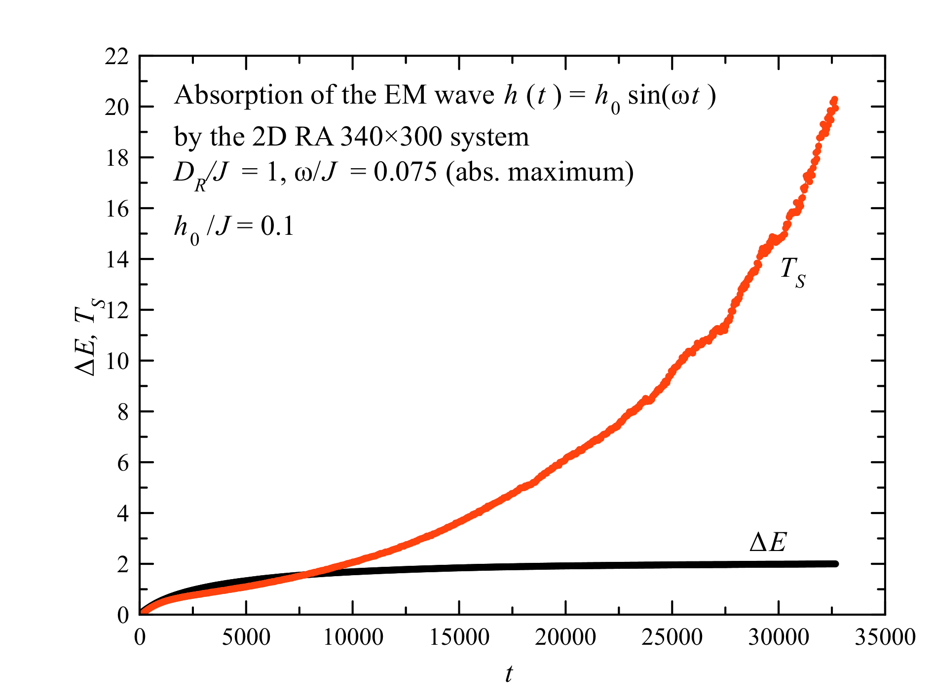
Figure 1: Time dependence of the absorbed microwave energy $\Delta E$ and of the spin temperature $T_{s}$ in the RA ferromagnet.

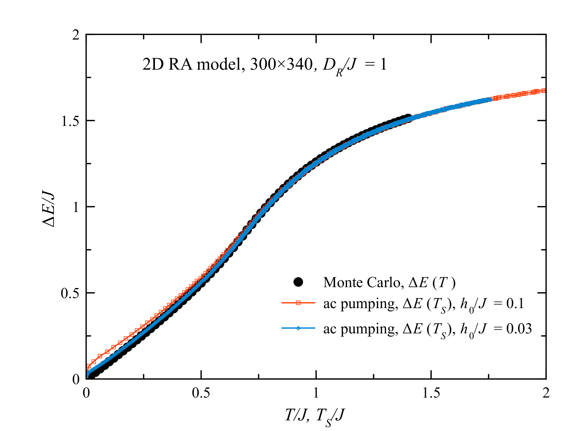
Figure 2: Absorbed energy vs Monte Carlo temperature $T$ and the spin temperature $T_{s}$.

This inconvenience can be cured by the recently proposed procedure of energy correction Garanin that can be performed from time to time to bring the system’s energy back to the expected target value. This procedure consists in a (small) rotation of each spin towards or away from the respective effective field

$$\delta{\bf s}_{i}=\xi{\bf s}_{i}\times({\bf s}_{i}\times{\bf H}_{{\rm eff},i}),$$ (14)

with $\xi$ chosen such that the ensuing energy change $\delta E=\xi\sum_{i}({\bf s}_{i}\times{\bf H}_{{\rm eff},i})$ has a required value. In the case of a free conservative dynamics, one has $\delta E=E_{0}-E$, where $E_{0}$ is the initial energy that must be conserved and $E$ is the current energy that differes from $E_{0}$ because of the accumulation of numerical errors.

In our first experiment with the ac pumping, the situation with the energy conservation is the following. The absorbed energy $E_{\mathrm{abs}}(t)=\int_{0}^{t}dt^{\prime}P_{\mathrm{abs}}(t^{\prime})$ is robust because any portion of the absorbed energy that has been counted does not change. On the contrary, the energy of the system $E\equiv\mathcal{H}$ changes because of numerical errors, even in the absence of pumping. If it changes significantly, then it begins to affect the absorbed power and the whole computation breaks down. Thus the energy of the system must be corrected so that the energy change $\Delta E(t)=E(t)-E_{0}$ is equal to the absorbed energy $E_{\mathrm{abs}}(t)$. This implies $\delta E=E_{\mathrm{abs}}-\Delta E$ in the energy-correcting transformation. In the case of pumping, this transformation should be done at the time moments when $\mathbf{h}(t)=0$, to avoid the ac field making a contribution to the energy. In this work, it was done each time a period of the pumping was completed.

In our second experiment with the free conservative dynamics and FDT, energy correction also was done with fixed time intervals. In this experiment, however, one could do a Monte Carlo update instead of correcting energy, to remove the energy drift. In both experiments, the computation time was not limited by any accuracy factors.

As the ODE solver, the fifths-order Runge-Kutta method with the time step $\delta t=0.1$ was used. As the computational tool, we employed Wolfram Mathematica with compilation of heavy-duty routines into C++ code using a C compiler installed on the computer. Most of the computations were performed on our Dell Precision Workstation having 20 cores. The computation in the first numerical experiment was not parallelized. For the second experiment, to better deal with fluctuations, we ran identical parallel computations on 16 cores available under our Mathematica licence and averaged the results. In computations, we set $J$ and all physical constants to one. The time $t$ is given in the units of $\hbar/J$.

IV Numerical results

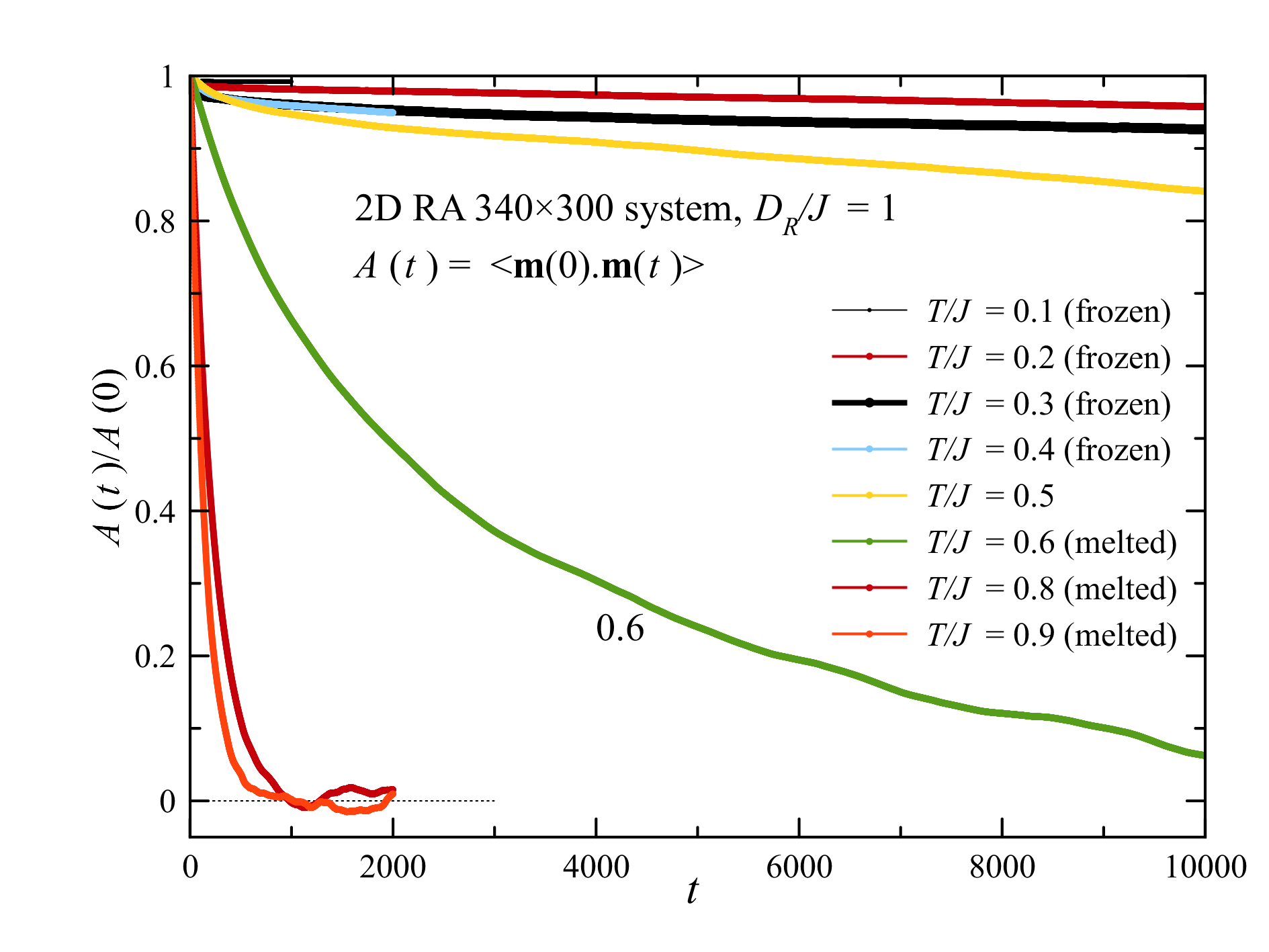
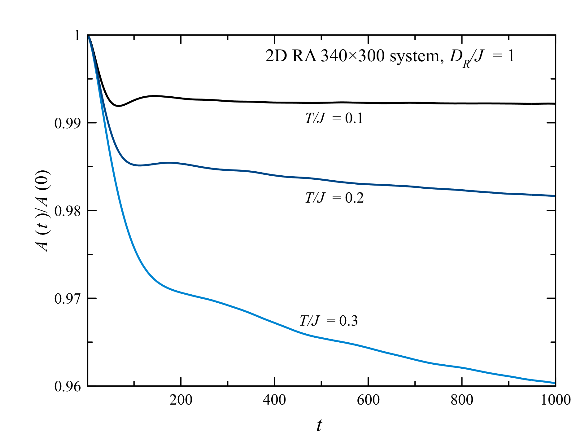
Figure 3: Autocorrelation function of the total spin at different temperatures temperatures. Upper panel: wide temperature range. Lower panel: low temperatures.

IV.1 Pumping, nonlinearity, heating

Pumping an isolated system during a long time increases its energy, that is, results in heating. For realistically small ac amplitudes, $h_{0}/J\lll 1$, the computation times required to reach a significant heating are prohibitively long. A spectacular heating can be reached for the extremely high ac amplitude $h_{0}/J=0.1$, although it requires a very long computation time. The results are shown in Fig. 1. At long times, the energy change of the system $\Delta E$ (equal to the absorbed energy $E_{\mathrm{abs}}$) reaches its maximal value corresponding to a total disordering of spins. In this state, the absorbed power is close to zero and the saturation is complete. The dynamical spin temperature $T_{S}$ defined by Eq. (4) reaches large values, as it should be. For $h_{0}/J=0.03$ that is also too large, a very long computation allowed to reach the temperature $T_{S}\approx 1.75J$.

The existence of the dynamic spin temperature $T_{S}$ allows to check if the state of the system is equilibrium during the energy-absorption process. In Fig. 2 the results above for $\Delta E(t)$ and $T_{S}(t)$ are parametrically replotted and compared with the dependence $\Delta E(T)$ computed by Monte Carlo. The parametric plots $\Delta E(T_{S})$ for $h_{0}/J=0.1$ and 0.03 perfectly coincide everywhere except the smallest $T_{S}$ where the $h_{0}/J=0.1$ curve bulges. For the $h_{0}/J=0.03$ the bulging also exists but is rather small. Both of these curves are in a good accord with the Monte Carlo curve $\Delta E(T)$. This result strongly suggests that as the RA magnet is absorbing the energy, the latter goes to all modes and the equipartition of the energy is reached. It is remarkable that the system is in equilibrium even for the huge ac amplitude $h_{0}/J=0.1$, except for the short times. For the realistically weak ac amplitudes, the equilibrium in the magnetic system should be complete.

The magnetic system being in equilibrium and having a particular spin temperature $T_{S}$ during the absorption of the microwave energy allows one to set up a single differential equation for the temperature that describes the whole process. Expressing the time derivative of the system’s energy in Eq. (3) via the heat capacity of the magnetic system $C$ and the time derivative of the spin temperature, one obtains

$$\dot{\mathcal{H}}(t)=C\dot{T}=P_{\mathrm{abs}}(\omega,T)$$ (15)

that results in a closed equation for $T(t)$

$$\dot{T}=\frac{P_{\mathrm{abs}}(\omega,T)}{C(T)}.$$ (16)

Thus, it is sufficient to compute the heat capacity of the spin system $C(T)$ by Monte Carlo and compute the absorbed power $P_{\mathrm{abs}}(\omega.T)$ at different temperatures to be able to solve the problem of heating and the resonance saturation numerically in no time! As the realistic ac field amplitudes are rather small, one can find $P_{\mathrm{abs}}(\omega.T)$ in the linear regime with the help of FDT. After the numerical solution of Eq. (16) is obtained, one can compute the absorbed energy by integration:

$$E_{\mathrm{abs}}(t)=\int_{0}^{t}dt^{\prime}P_{\mathrm{abs}}\left[\omega,T(t^{\prime})\right].$$ (17)

As the spin-lattice relaxation is rather fast, one can add the heat capacity of the lattice to that of the magnetic system. This will alleviate the negative action of heating and increase absorption. Also, the energy can flow from the magnetic particles to the dielectric matrix by heat conduction. However, this process is slow and it cannot transfer a significant energy during the time of the microwave pulse.

IV.2 Microwave power absorption by FDT

In the second numerical experiment, we ran conservative dynamical evolution of the states created by Monte Carlo at the temperatures $T/J=0.1\div 1.0$ in step of 0.1. The computation was performed in parallel on 16 processor cores until $t=t_{\max}=50000$ in most cases. From the computed dependences $\mathbf{m}(t)$ the autocorrelation function $A(t)$ entering Eq. (13) was computed and the results were averaged over the cores. Computations on our Dell Precision Workstation took five days for each temperature. The normalized autocorrelation functions $A(t)/A(0)$ at different temperatures are shown in Fig. 3. These dependences have different forms at low and elevated temperatures that can be interpreted in terms of glassy physics. Below $T/J\approx 0.6$, spins are frozen and $A(t)$ is decreasing very slowly, apparently due to bunches of spins (IM domains) crossing anisotropy barriers due to thermal agitation.

There is a fundamental unsolved question whether the RA system can be described in terms of IM domains whose magnetic moments become blocked at low temperatures due to barriers or it is a true spin-glass state. Shand-JAP2005 Since our focus is on the absorption of microwaves we do not attempt to answer this question here. In Eq. (13) for the absorbed power, the low-frequency part of $A(\omega)$ is suppressed by the factor $\omega^{2}$, so that the long-time physics is irrelevant for the absorption.

The contribution to the absorbed power comes from the short-time part of $A(t)$ that is shown in the lower panel of Fig. 3. There is an initial steep descent of $A(t)$ ending in a quasi-plateau at low temperatures. This steep descent can be interpered as caused by dephasing of precession of different IM domains in their potential wells. This precession with a quasi-continuous spectrum of frequencies is what ensures the absorption of the microwave power in a broad frequency range. As each IM domain remains precessing in its own potential well, $A(t)$ cannot change by a large amount. The latter requires flipping of IM domains over the barriers that happens at higher temperatures.

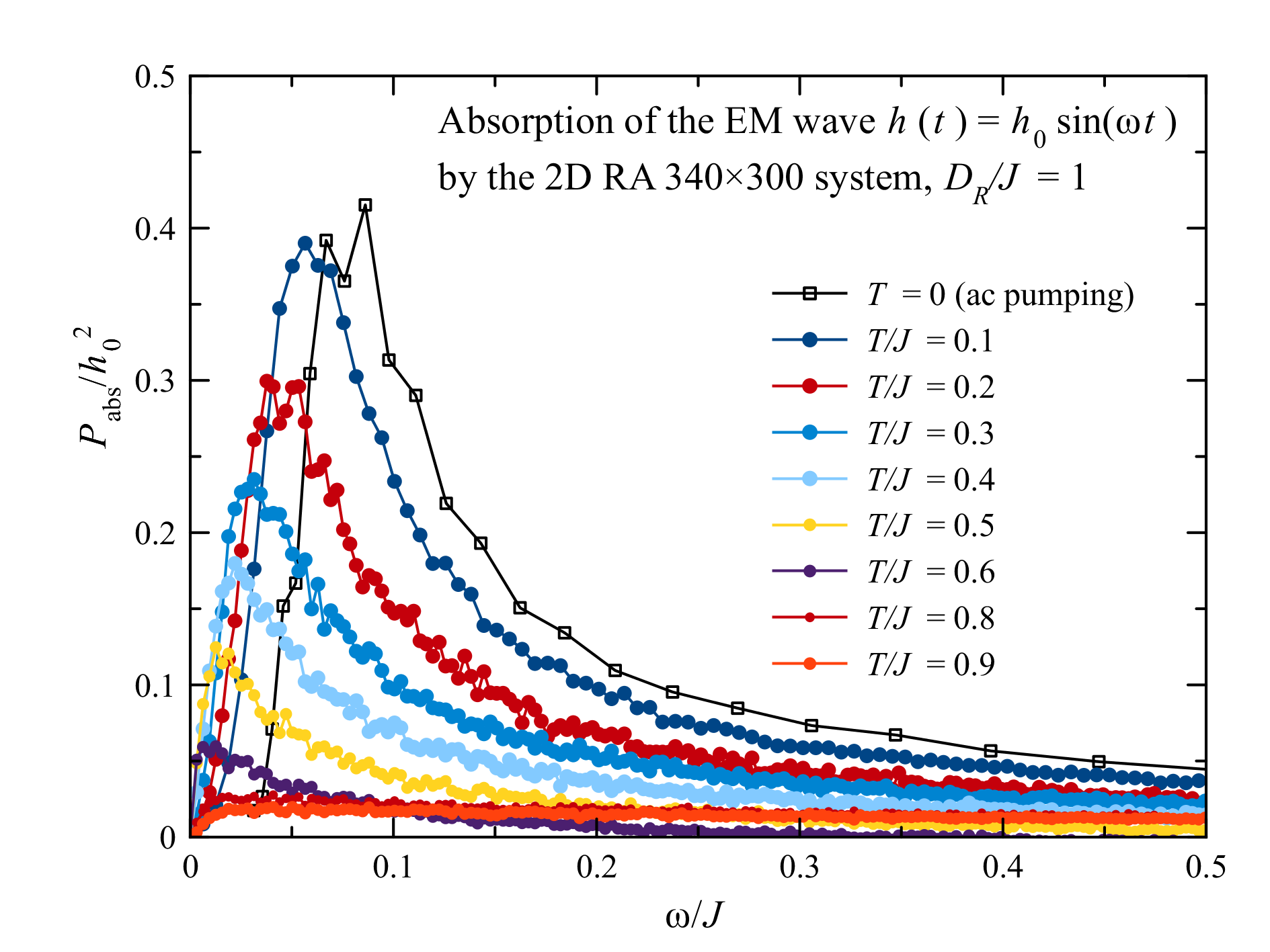
Figure 4: Frequency dependence of the absorbed microwave power at different temperatures. The ac pumping result at $T=0$ of Ref. GC-PRB2021, is shown for comparison.

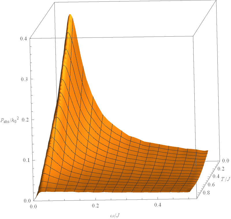
Figure 5: Dependence of the absorbed microwave power on the temperature and frequency.

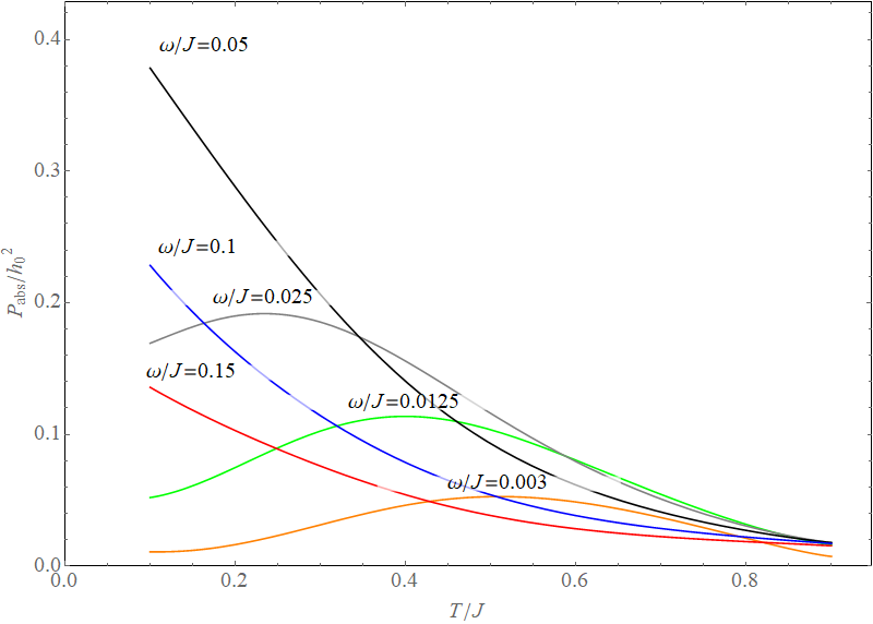
Figure 6: Temperature dependence of the absorbed microwave power at different frequencies.

Making the Fourier transform of $A(t)$ and using Eq (13), one obtaines the absorbed power $P(\omega)$ that is shown in Fig. 4. One can see that the absorption curve is getting depressed with increasing the temperature, until the absorption peak vanishes when the glassy state of the system melts. This is similar to what one observes in a system of independent resonating spins (or magnetic particles): The more thermally excited are the spins, the less they absorb. Absorption is maximal if the spins are in their ground states at $T=0$.

Fig. 5 shows the same data presented in a 3D form as $P_{\mathrm{abs}}(\omega,T)$ with the help of the approximation using Bezier functions implemented in Wolfram Mathematica.

Having built the approximation for $P_{\mathrm{abs}}(\omega,T)$, one can plot the curves $P_{\mathrm{abs}}(T)$ for different $\omega$, as shown in Fig. 6. Since the maximum of $P_{\mathrm{abs}}(\omega)$ is shifting to the left with increasing $T$, the curves $P_{\mathrm{abs}}(T)$ have a maximum for smaller $\omega$. The dependences $P_{\mathrm{abs}}(T)$ can be used in the equation for the spin temperature, Eq. (16).

V Discussion

Earlier we have shown GC-PRB2021 that RA magnets can be strong broadband absorbers of the microwave power. In this paper we have studied the temperature dependence of the power absorption. Our results answer two questions, both related to applications of microwave absorbers. The first one is a direct question of how the absorption by RA magnets depends on their temperature when they are heated by an independent source. It is answered by Fig. 4 which shows a decrease of the absorption with increasing temperature in a broad frequency range, making the system basically transparent for the microwaves at a sufficiently high temperature.

The second question is a response of the RA magnet to a microwave pulse of high power. We have shown that during the pulse, the spin system is in equilibrium and can be described in terms of the spin temperature. As typical times of spin-phonon transitions are much shorter than a microsecond, the spin system also equilibrates with the lattice. On the other hand, the time required for the flow of heat out of a dielectric layer of thickness $l$, containing densely packed RA magnets, can be estimated as $t\sim(\rho cl^{2})/k$, where $\rho$, $c$, and $k$ are the average mass density, the specific heat, and the thermal conductivity of the layer. For the layer of a few-millimeter thickness it is in the ballpark of a fraction of a second or longer, depending on the substrate. Thus, for the microwave pulses shorter than this time, the heat-conductivity mechanism is irrelevant.

A sufficiently strong pulse of microwave energy directed at such a layer, having duration in the range from microseconds to milliseconds, can greatly diminish the absorption capacity of the layer during the action of the pulse, making it transparent for the microwaves. During that time, if the layer is covering a metallic surface, the microwaves in a broad frequency range would pass it with the minimum absorption and would be reflected by the metal. This effect can be minimized by making the layer densely packed with metallic RA magnets electrically insulated from each other by a very thin dielectric coating. High thermal conductivity of such a system would greatly increase its cooling via heat conduction and would make its absorbing capabilities more resistant to high-power pulses of direct microwave energy.

References

- (1) E. M. Chudnovsky, Random Anisotropy in Amorphous Alloys, Chapter 3 in the Book: Magnetism of Amorphous Metals and Alloys, edited by J. A. Fernandez-Baca and W.-Y. Ching, pages 143-174 (World Scientific, Singapore, 1995).
- (2) E. M. Chudnovsky and J. Tejada, Lectures on Magnetism (Rinton Press, Princeton, New Jersey, 2006).
- (3) T. C. Proctor, E. M. Chudnovsky, and D. A. Garanin, Scaling of coercivity in a 3d random anisotropy model, Journal of Magnetism and Magnetic Materials, 384, 181-185 (2015).
- (4) Y. Imry and S.-k. Ma, Random-field instability of the ordered state of continuous symmetry, Physical Review Letters 35, 1399-1401 (1975).
- (5) E. M. Chudnovsky, W. M. Saslow, and R. A. Serota, Ordering in ferromagnets with random anisotropy, Physical Review B 33, 251-261 (1986).
- (6) R. A. Serota and P. A. Lee, Continuous-symmetry ferromagnets with random anisotropy, Journal of Applied Physics 61, 3965-3967 (1987).
- (7) B. Dieny and B. Barbara, XY model with weak random anisotropy in a symmetry-breaking magnetic field, Physical Review B 41, 11549-11556 (1990).
- (8) R. Dickman and E. M. Chudnovsky, chain with random anisotropy: Magnetization law, susceptibility, and correlation functions at , Physical Review B 44, 4397-4405 (1991).
- (9) D. A. Garanin, E. M. Chudnovsky, and T. Proctor, Random field xy model in three dimensions, Physical Review B 88, 224418-(21) (2013).
- (10) T. C. Proctor, D. A. Garanin, and E. M. Chudnovsky, Random fields, Topology, and Imry-Ma argument, Physical Review Letters 112, 097201-(4) (2014).
- (11) E. M. Chudnovsky and D. A. Garanin, Topological order generated by a random field in a 2D exchange model, Physical Review Letters 121, 017201-(4) (2018).
- (12) G. Suran, E. Boumaiz, and J. Ben Youssef, Experimental observation of the longitudinal resonance mode in ferromagnets with random anisotropy, Journal of Applied Physics 79, 5381 (1996).
- (13) S. Suran and E. Boumaiz, Observation and characteristics of the longitudinal resonance mode in ferromagnets with random anisotropy, Europhysics Letters 35, 615-620 (1996).
- (14) S. Suran and E. Boumaiz, Longitudinal resonance in ferromagnets with random anisotropy: A formal experimental demonstration, Journal of Applied Physics 81, 4060 (1997).
- (15) G. Suran, Z, Frait, and E. Boumaz, Direct observation of the longitudinal resonance mode in ferromagnets with random anisotropy, Physical Review B 55, 11076-11079 (1997).
- (16) S. Suran and E. Boumaiz, Longitudinal-transverse resonance and localization related to the random anisotropy in a-CoTbZr films, Journal of Applied Physics 83, 6679 (1998).
- (17) R. D. McMichael, D. J. Twisselmann, and A. Kunz, Localized ferromagnetic resonance in inhomogeneous thin film, Physical Review Letters 90, 227601-(4) (2003).
- (18) G. de Loubens, V. V. Naletov, O. Klein, J. Ben Youssef, F. Boust, and N. Vukadinovic, Magnetic resonance studies of the fundamental spin-wave modes in individual submicron Cu/NiFe/Cu perpendicularly magnetized disks, Physical Review Letters 98, 127601-(4) (2007).
- (19) C. Du, R. Adur, H. Wang, S. A. Manuilov, F. Yang, D. V. Pelekhov, and P. C. Hammel, Experimental and numerical understanding of localized spin wave mode behavior in broadly tunable spatially complex magnetic configurations, Physical Review B 90, 214428-(10) (2014).
- (20) W. M. Saslow and C. Sun, Longitudinal resonance for thin film ferromagnets with random anisotropy, Physical Review B 98, 214415-(6) (2018).
- (21) P. Monod and Y. Berthier, Zero field electron spin resonance of Mn in the spin glass state, Journal of Magnetism and Magnetic Materials 15-18,149-150 (1980).
- (22) J. J. Prejean, M. Joliclerc, and P. Monod, Hysteresis in CuMn: The effect of spin orbit scattering on the anisotropy in the spin glass state, Journal de Physique (Paris) 41, 427-435 (1980).
- (23) H. Alloul and F. Hippert, Macroscopic magnetic anisotropy in spin glasses: transverse susceptibility and zero field NMR enhancement, Journal de Physique Lettres 41, L201-204 (1980).
- (24) S. Schultz, E .M. Gulliksen, D. R. Fredkin, and M.Tovar, Simultaneous ESR and magnetization measurements characterizing the spin-glass state, Physical Review Letters 45, 1508-1512 (1980).
- (25) E. M. Gullikson, D. R. Fredkin, and S. Schultz, Experimental demonstration of the existence and subsequent breakdown of triad dynamics in the spin-glass CuMn, Physical Review Letters 50, 537-540 (1983).
- (26) A. Fert and P. M. Levy, Role of anisotropic exchange interactions in determining the properties of spin-glasses, Physical Review Letters 44,1538-1541 (1980).
- (27) P. M. Levy and A. Fert, Anisotropy induced by nonmagnetic impurities in CuMn spin-glass alloys, Physical Review B 23, 4667 (1981).
- (28) C. L. Henley, H. Sompolinsky, and B. I. Halperin, Spin-resonance frequencies in spin-glasses with random anisotropies, Physical Review B 25, 5849-5855, (1982).
- (29) B. I. Halperin and W. M. Saslow, Hydrodynamic theory of spin waves in spin glasses and other systems with noncollinear spin orientations, Physical Review B 16, 2154-2162 (1977).
- (30) W. M. Saslow, Anisotropy-triad dynamics, Physical Review Letters 48, 505-508 (1982).
- (31) D. A. Garanin and E. M. Chudnovsky, Absorption of microwaves by random-anisotropy magnets, Physical Review B 103, 214414-(11) (2021).
- (32) I. Y. Korenblit and E. F. Shender, Spin glasses and nonergodicity, Soviet Physics Uspekhi 32, 139-162 (1989).
- (33) D. A. Garanin and E. M. Chudnovsky, Ordered vs. disordered states of the random-field model in three dimensions, European Journal of Physics B 88, 81-(19) (2015).
- (34) J. V. I. Jaakko et al., Magnetic nanocomposites at microwave frequencies, in a book: Trends in Nanophysics, edited by V. Barsan and A. Aldea, pages 257-285 (Springer, New York, 2010).
- (35) X. Zeng, X. Cheng, R. Yu, and G. D. Stucky, Electromagnetic microwave absorption theory and recent achievements in microwave absorbers, Carbon 168, 606-623 (2020).
- (36) D. A. Garanin, Energy balance and energy correction in dynamics of classical spin systems, Condensed Matter arXiv:2106.14689.
- (37) W. B. Nurdin and K.-D. Schotte, Dynamical temperature for spin systems, Physical Review E 61, 3579-3582 (2000).
- (38) P. M. Shand, C. C. Stark, D. Williams, M. A. Morales, T. M. Pekarek, and D. L. Leslie-Pelecky, Spin glass or random anisotropy?: The origin of magnetically glassy behavior in nanostructured GdAl2, Journal of Applied Physics 97, 10J505-(3) (2005).