On linear power corrections in certain collider observables

Abstract

We study linear power corrections ${\cal O}(\Lambda_{\rm QCD}/Q)$ to certain collider observables. We present arguments that prove that such corrections cannot appear in observables that are inclusive with respect to QCD radiation, such as total cross sections as well as rapidity and transverse momentum distributions of color-neutral particles. Although our calculations are carried out in a simplified framework, our arguments and conclusions are applicable, with some reservations, to processes both at lepton and hadron colliders. We also show how an improved understanding of the origin of linear power corrections allows us to simplify their calculation. As an application, we compute the leading non-perturbative corrections to the $C$-parameter and the thrust in $e^{+}e^{-}$ annihilation in a generic three-jet configuration.

1 Introduction

An important part of the LHC physics program consists in the exploration of phenomena that occur at distances that are between a hundred and a thousand times smaller than the size of the proton. Thanks to the celebrated properties of Quantum Chromodynamics (QCD) such as asymptotic freedom and factorization, physics at such distances can be described using perturbation theory, where elusive quarks and gluons play the role of fundamental physical degrees of freedom.

Corrections to this perturbative picture are expected to be small, suppressed by ratios of the non-perturbative QCD parameter $\Lambda_{\rm QCD}\sim 0.3~{}{\rm GeV}$ and the typical energy scale $Q$ of the process (or observable) under consideration. This hard scale $Q$ typically ranges from a few tens to a few hundred GeV. It follows that these non-perturbative effects may change perturbative predictions by a relative amount proportional to $(\Lambda_{\rm QCD}/Q)^{n}\sim(0.01)^{n}-(0.001)^{n}$ which, depending on the value of $Q$ and of the exponent $n$, varies from a percent for $n=1$ and $Q\sim 30~{}{\rm GeV}$ to a permille and even smaller values for larger values of $Q$ and $n$.

Perturbative predictions for cross sections and distributions, on the other hand, are controlled by powers of the strong coupling constant $\alpha_{s}(Q)\sim 0.1$ for $Q\sim 30-100~{}{\rm GeV}$. Currently, perturbative computations are often performed to second or even third order in the expansion in $\alpha_{s}$, leading to theoretical predictions for hard processes which are typically accurate to within one to ten percent Heinrich:2020ybq . Further development of methods for perturbative calculations in QCD may improve the precision of such theoretical predictions, perhaps by about an order of magnitude. If this happens even for a few selected processes and observables, perturbative predictions at this precision will have to be supplemented with non-perturbative corrections provided that $\mathcal{O}((\Lambda_{\rm QCD}/Q)^{n})$ contributions with $n=1$ exist for a particular process or observable. On the other hand, non-perturbative corrections with $n>1$ are too small to be of any relevance for most hard processes at the LHC.

For color-singlet decay rates, deep-inelastic scattering structure functions and inclusive decays of heavy quarks Bigi:1993fe , it is well-known that operator product expansion techniques allow one to conclude that fully inclusive observables do not receive linear power corrections. However, it is currently not known how to generalize these results to more differential observables and to the case of hadron-hadron collisions. Indeed, at present there is no full theory of non-perturbative corrections to short-distance processes at lepton and hadron colliders. It is then not possible to predict the exponent $n$ for a generic process or observable, let alone compute the contribution of $O((\Lambda_{\rm QCD}/Q)^{n})$ terms precisely. However, it is well-understood that one source of non-perturbative corrections is present within perturbation theory itself. Indeed, the appearance of the Landau pole in the strong coupling constant leads to an intrinsic ambiguity when integrating over soft momenta. Since such an ambiguity will have to cancel with contributions that arise from physics beyond perturbation theory, it can be used as an estimate of, at least, some non-perturbative contributions.

It is well-known that the ambiguity related to the appearance of the Landau pole can be studied within the approximation of a large (and negative) number of massless fermion species (see Ref. Beneke:1998ui for a review). This approach is particularly simple if no gluons appear in a given process at leading order. Indeed, in such cases the appearance of linear power corrections can be investigated by computing $\mathcal{O}(\alpha_{s})$ corrections to the process (and observable) under consideration that originate from virtual exchanges and real emissions of massive gluons, in the limit of a small gluon mass $\lambda$, see Ref. Beneke:1998ui . The presence of terms that are linear in $\lambda$ implies that a particular observable receives leading power corrections that are of the type $\mathcal{O}(\Lambda_{\rm QCD}/Q)$, while their absence can be interpreted as an indication that non-perturbative corrections are further suppressed.

In the context of high-energy collider physics, early studies of linear power corrections were mostly focused on studying shape variables in electron-positron collisions Manohar:1994kq ; Webber:1994cp ; Akhoury:1995sp ; Dokshitzer:1995zt ; Nason:1995np ; Dokshitzer:1995qm ; Dasgupta:1996ki ; Beneke:1997sr ; Dokshitzer:1997ew ; Dokshitzer:1997iz ; Dokshitzer:1998pt , on the heavy-quark mass definition Beneke:1994sw ; Bigi:1994em , on the Drell-Yan process Beneke:1995pq ; Dasgupta:1999zm ; Korchemsky:1996iq and on jets Korchemsky:1994is ; Dasgupta:2007wa . Recently, first attempts were made to extend such studies to more complicated processes that could be considered as proxies for realistic processes at hadron colliders. In particular, appearances of linear power corrections in top production and decay processes and in the transverse momentum distribution of the $Z$ bosons produced in photon-hadron collisions were studied in Refs. FerrarioRavasio:2018ubr ; FerrarioRavasio:2020guj , respectively. In both cases, calculations were performed numerically for finite values of the gluon mass $\lambda$. The presence or absence of linear power corrections was established by a numerical extrapolation to vanishing values of $\lambda$.

In the case of the $Z$ transverse momentum distribution studied in Ref. FerrarioRavasio:2020guj , no evidence of linear power corrections was found. Although this result is fully sufficient for phenomenological purposes, it is interesting to understand if the presence or absence of such linear corrections in hard processes can be deduced on more general grounds. This is what we set out to do in this paper. Unfortunately, we are not yet able to perform an analysis of fully realistic processes since we have to restrict ourselves to cases where there are no gluons at leading order. Apart from this rather substantial restriction, we keep our discussion general. Whenever we are interested in a process that does contain gluons at leading order (e.g. the $Z$ transverse momentum distribution, or $e^{+}e^{-}$ event shapes in the three-jet region) we follow the approach of Ref. FerrarioRavasio:2020guj and use photons as proxies for hard gluons. Our main findings can be stated as follows:

• no linear powers of $\lambda$ arise from virtual corrections in generic hard processes with massless partons;

• observables that are inclusive with respect to momenta of colored final state particles do not receive ${\cal O}(\lambda)$ and, therefore, ${\cal O}(\Lambda_{\rm QCD}/Q)$ power corrections. Observables of this type include e.g. total cross sections as well as kinematic distributions of colorless particles.

From these findings it immediately follows that no linear power corrections appear in the inclusive Drell-Yan cross section Beneke:1995pq and in the rapidity distribution of the Drell-Yan pair Dasgupta:1999zm , at least away from the kinematic boundaries. Similarly, they also imply that the $Z$ transverse momentum distribution computed in the simplified model of photon-hadron collisions studied in Ref. FerrarioRavasio:2020guj also does not receive linear power corrections, even if rapidity cuts on the $Z$ boson are applied.

Our results have interesting implications for event-shape studies in $e^{+}e^{-}$ annihilation. Recently, this topic has received renewed attention in relation to the extractions of the strong coupling constant $\alpha_{s}$ from event shapes. Indeed, it was argued in Ref. Luisoni:2020efy that a better control on non-perturbative corrections is crucial for a reliable determination of $\alpha_{s}$. In particular, in Ref. Luisoni:2020efy the standard approach to computing power corrections, that consists in extrapolating them from the two-jet to the three-jet region, was criticized. By considering shape variables like the $C$-parameter that exhibit two Sudakov regions (one near the two-jet limit and the other at the three-jet symmetric point), the authors of Ref. Luisoni:2020efy argued that the coefficient of the linear power correction near the two-jet region cannot be reliably extrapolated to the three-jet one. With our formalism, we can compute the coefficient of the power corrections in the three-jet region for several shape variables, irrespective of the presence of Sudakov regions.

This paper is organized as follows. In Section 2 we study non perturbative corrections in a toy model, namely the production of two scalar color-charged particles in the decay of a massive vector boson. Within this toy model, we argue that the decay rate in this case is free of linear ${\cal O}(\Lambda_{\rm QCD}/Q)$ corrections. Rather than presenting new results, the purpose of this section is to illustrate basic features of our approach and to provide arguments that can be generalized to more complex cases. Such generalization is discussed in Section 3, which is devoted to more complex processes with additional hard particles in both the initial and final states. There, we generalize arguments given in Section 2 and argue that also in more complex cases linear ${\cal O}(\Lambda_{\rm QCD}/Q)$ terms are not present for observables that are inclusive with respect to QCD radiation.

In Sections 4 and 5 we consider the implications of our result for the calculation of shape variables in $e^{+}e^{-}$ annihilation. In particular, in Section 4 we discuss a specific observable, namely the $C$-parameter, and show how our formalism can be applied to compute non-perturbative corrections to it in an approximation where the splitting of a massive gluon into a $q\bar{q}$ pair is neglected. In Section 5 we present a general framework for dealing with a broader class of shape variables. Using this framework, we compute linear power corrections to both the thrust and the $C$-parameter distributions and compare these results with a numerical calculation at finite $\lambda$, extrapolated to $\lambda\to 0$. We find consistent results, confirming our analytical findings. We conclude in Section 6.

This paper also contains several appendices. In Appendix A we describe the computation of integrals relevant for our study. In Appendix B, we detail the analytic calculation of the various integrals that we use in our analysis of the $C$-parameter in Section 4. In Appendix C, we report technical details of the calculation of shape variables in the large-$n_{f}$ limit that we discuss in Section 5. Finally, in Appendix D we study non-perturbative corrections to the $C$-parameter in the two-jet limit.

2 A toy model: vector-boson decay to scalars

In this section, we consider the decay of a spin-one boson into two colored charged scalars $\phi$. Our goal is to understand linear power corrections in this model and present arguments that, on the one hand, can be easily verified in this simple case and, on the other hand, are sufficiently general to be applicable in more complex situations. Because of this, we refrain as much as possible from using the exact form of the various matrix elements relevant for this calculation, and instead focus on their general structure.

We investigate power corrections to the process

$$V(q)\to\phi(p_{1})+\bar{\phi}(p_{2}).$$ (1)

Following the discussion in the introduction, we do this by computing ${\cal O}(\alpha_{s})$ corrections to this process in a QCD-like theory where the gluon has a small mass $\lambda$, and by checking whether or not such corrections contain terms that are linear in $\lambda$. To keep our analysis as simple as possible, in this section we only consider the total decay rate. We will discuss more complicated processes and observables in Section 3. As stated earlier, we only consider the case of massless scalars, $p_{1}^{2}=p_{2}^{2}=0$.

We begin with the analysis of virtual corrections. There are two contributions that need to be studied – the wave-function renormalization constant for the external $\phi$ particles and the one-loop matrix element. We start with the former. We work in dimensional regularization, define the space-time dimension as $d=4-2\epsilon$, and use the Feynman gauge for simplicity. The scalar’s self-energy reads

$$\Sigma(p^{2})=(\sigma_{1}\,p^{2}+\sigma_{2}\,\lambda^{2})B(p,\lambda)+~{}{\rm terms~{}that~{}do~{}not~{}depend~{}on~{}}p^{2},$$ (2)

where

$$B(p,\lambda)=\int\frac{d^{d}k}{(2\pi)^{d}}\frac{1}{(k^{2}-\lambda^{2})(k+p)^{2}},$$ (3)

and $\sigma_{1,2}$ are two constants whose specific form is irrelevant for our discussion. Using Feynman parameters, $B(p,\lambda)$ can be written as

$$B(p,\lambda)=i\frac{\Gamma(\epsilon)}{(4\pi)^{d/2}}\int\limits_{0}^{1}\mathrm{d}x\,x^{-\epsilon}\left[\lambda^{2}-p^{2}(1-x)\right]^{-\epsilon}.$$ (4)

This representation makes it apparent that

$$B(p,\lambda)|_{p^{2}=0}\sim\lambda^{-2\epsilon},~{}~{}~{}~{}~{}~{}\lambda^{2}\left.\frac{\partial B(p,\lambda)}{\partial p^{2}}\right|_{p^{2}=0}\sim\lambda^{-2\epsilon},$$ (5)

which in turn implies that the wave-function renormalization constant $Z_{\phi}$ does not contain terms that are linear in $\lambda$.

We then move to the one-loop matrix element. There are three diagrams that contribute to it. Using the Passarino-Veltman reduction Passarino:1978jh , one can express this matrix element through four scalar integrals. Omitting color indices for simplicity, we schematically write

$$\begin{split}&{\cal M}_{1-\rm loop}(p_{1},p_{2},\lambda)=c\left(p_{1},p_{2},\lambda^{2}\right)C(p_{1},p_{2},\lambda)+b_{1}\left(p_{1},p_{2},\lambda^{2}\right)B(p_{1},\lambda)\\ &\quad\quad+b_{2}\left(p_{1},p_{2},\lambda^{2}\right)B(p_{2},\lambda)+b_{3}\left(p_{1},p_{2},\lambda^{2}\right)B(p_{1}+p_{2},0)+a\left(p_{1},p_{2},\lambda^{2}\right)A(\lambda),\end{split}$$ (6)

where $B(p,\lambda)$ is given in Eq. (3) and the other loop integrals are defined as

$$\begin{split}C(p_{1},p_{2},\lambda)=\int\frac{{\rm d}^{4}k}{(2\pi)^{4}}\frac{1}{(k^{2}-\lambda^{2})(k+p_{1})^{2}(k-p_{2})^{2}},~{}~{}~{}A(\lambda)=\int\frac{{\rm d}^{d}k}{(2\pi)^{d}}\frac{1}{(k^{2}-\lambda^{2})}.\end{split}$$ (7)

As indicated in Eq. (6), the coefficient functions $c,b_{1,2,3}$ and $a$ are rational functions of $\lambda^{2}$; this is a direct consequence of how the Passarino-Veltman reduction proceeds. It remains to consider the scalar integrals. Eq. (5) implies that $B(p_{1,2},\lambda)\sim\lambda^{-2\epsilon}$. Also, dimensional analysis dictates that $A\sim\lambda^{2-2\epsilon}$. These integrals cannot then generate odd powers of $\lambda$ upon expansion in both $\epsilon$ and $\lambda$. The case of the scalar triangle $C$ is less trivial. However, it is easy to see that it admits the following representation

$$C(p_{1},p_{2},\lambda)=\frac{i}{(4\pi)^{2}}\int\limits_{0}^{1}\frac{{\rm d}x}{q^{2}x+\lambda^{2}}\left[\ln\frac{q^{2}x}{\lambda^{2}}-i\pi\right].$$ (8)

Although it is straightforward to complete the integration over $x$ and express $C$ in terms of polylogarithmic functions, this is not necessary as the above representation makes it obvious that the function $C$ does not contain odd terms in the small-$\lambda$ expansion.

We then conclude that the behavior of the renormalized one-loop virtual amplitude in the limit of small $\lambda$ is described by the following formula

$${\cal M}^{\rm ren}_{1-\rm loop}(p_{1},p_{2},\lambda)=\omega_{1}(p_{1},p_{2})\ln^{2}\frac{q^{2}}{\lambda^{2}}+\omega_{2}(p_{1},p_{2})\ln\frac{q^{2}}{\lambda^{2}}+\omega_{3}(p_{1},p_{2})+{\cal O}(\lambda^{2}).$$ (9)

The logarithmic divergences in $\lambda^{2}$ are the usual soft-collinear singularities, that are canceled by analogous contributions in the real emission terms. Apart from that, Eq. (9) implies that the dependence on $\lambda$ in virtual corrections starts at $\mathcal{O}(\lambda^{2})$. We conclude that for the process $V\to\phi\bar{\phi}$ virtual corrections do not induce any linear sensitivity to infrared physics.

As the next step, we need to analyze the real-emission contribution

$$V(q)\to\phi(p_{1})+\bar{\phi}(p_{2})+g(k),$$ (10)

with $k^{2}=\lambda^{2}$. The amplitude of this process can be written as

$$\begin{split}{\cal M}(p_{1},p_{2},k)&=g_{s}T^{a}_{12}\left\{\frac{(2p_{1}+k)_{\mu}\epsilon^{\mu}}{(p_{1}+k)^{2}}\mathcal{M}_{0}(p_{1}+k,p_{2})\right.\\ &\left.-\frac{(2p_{2}+k)_{\mu}\epsilon^{\mu}}{(p_{2}+k)^{2}}\mathcal{M}_{0}(p_{1},p_{2}+k)+\epsilon_{\mu}\mathcal{M}_{3}^{\mu}(p_{1},p_{2},k)\right\}.\end{split}$$ (11)

The two first terms on the right hand side describe emissions by external particles while the third one describes “structure-dependent” radiation. In Eq. (11), $g_{s}$ is the strong coupling, $T^{a}_{12}$ is the generator of the $SU(3)$ color algebra in the fundamental representation and $\epsilon$ is the polarization vector of the gluon. Also, $\mathcal{M}_{0}(p_{1},p_{2})$ is the color-stripped matrix element with no extra emissions, while the structure of $\mathcal{M}_{3}$ will be discussed in the following.

It is obvious that if the emitted gluon is resolved, the amplitude squared and the phase space can be expanded in powers of $\lambda^{2}$. The situation is, however, more delicate in the soft and collinear regions where a) the amplitude develops singularities in the $\lambda\to 0$ limit and b) one becomes sensitive to restrictions on the phase space induced by the gluon mass that can be linear in $\lambda$. These regions are a potential source of linear power corrections and we now study them in detail.

We begin by discussing the emission of a soft gluon. Simple power counting arguments show that this region could give rise to linear power corrections. Indeed, consider a situation where the gluon energy $\omega$ is comparable to $\lambda$, $\omega\sim\lambda$. The phase space is proportional to $\omega\,{\rm d}\omega\,\beta\,\theta(\omega-\lambda)$, with $\beta=\sqrt{1-\lambda^{2}/\omega^{2}}$. Since for small $\lambda$ the real emission amplitude is expandable in powers of $\omega$ starting with $\mathcal{M}\sim 1/\omega$, linear terms in $\lambda$ could potentially be generated. To see whether this is the case, we need to study both the matrix element and the phase space in more detail. The power counting argument implies that linear power corrections can only originate from next-to-leading terms in the small-$\omega$ expansion of both the matrix element squared and the phase space. We now discuss how to compute them.

We consider first the matrix element, and construct an expansion of the real-emission amplitude in powers of $k$ Low:1958sn ; landau . We write

$$\begin{split}{\cal M}(p_{1},p_{2},k)&=g_{s}T^{a}_{12}\left\{\left[\frac{(2p_{1}+k)^{\mu}}{(p_{1}+k)^{2}}-\frac{(2p_{2}+k)^{\mu}}{(p_{2}+k)^{2}}\right]\mathcal{M}_{0}(p_{1},p_{2})\right.\\ &\left.+\frac{p_{1}^{\mu}}{(p_{1}k)}\frac{\partial\mathcal{M}_{0}}{\partial p_{1}^{\alpha}}k^{\alpha}-\frac{p_{2}^{\mu}}{(p_{2}k)}\frac{\partial\mathcal{M}_{0}}{\partial p_{2}^{\alpha}}k^{\alpha}+\mathcal{M}_{3}^{\mu}(p_{1},p_{2},0)+{\cal O}(k)\right\}\epsilon_{\mu}.\end{split}$$ (12)

We can determine $\mathcal{M}_{3}^{\mu}$ if we require that the above expression satisfies the Ward identity which means that upon replacing $\epsilon^{\mu}$ with $k^{\mu}$ in Eq. (12) we should get zero. We find that this is achieved if the following condition is satisfied

$$\frac{\partial\mathcal{M}_{0}}{\partial p_{1}^{\alpha}}k^{\alpha}-\frac{\partial\mathcal{M}_{0}}{\partial p_{2}^{\alpha}}k^{\alpha}+\mathcal{M}_{3}^{\alpha}k_{\alpha}=0.$$ (13)

It follows that

$$\mathcal{M}_{3}^{\alpha}=-\frac{\partial\mathcal{M}_{0}}{\partial p_{1}^{\alpha}}+\frac{\partial\mathcal{M}_{0}}{\partial p_{2}^{\alpha}}.$$ (14)

The amplitude expanded to first subleading order in $k$ then reads

$$\begin{split}{\cal M}(p_{1},p_{2},k)&=g_{s}T^{a}_{12}\left\{\left[\frac{(2p_{1}+k)_{\mu}}{(p_{1}+k)^{2}}-\frac{(2p_{2}+k)_{\mu}}{(p_{2}+k)^{2}}\right]\mathcal{M}_{0}(p_{1},p_{2})\right.\\ &\left.+\frac{p_{1,\mu}}{(p_{1}k)}\frac{\partial\mathcal{M}_{0}}{\partial p_{1}^{\alpha}}k^{\alpha}-\frac{p_{2,\mu}}{(p_{2}k)}\frac{\partial\mathcal{M}_{0}}{\partial p_{2}^{\alpha}}k^{\alpha}-\left(\frac{\partial\mathcal{M}_{0}}{\partial p_{1}^{\mu}}-\frac{\partial\mathcal{M}_{0}}{\partial p_{2}^{\mu}}\right)+\mathcal{O}(k)\right\}\epsilon^{\mu}.\end{split}$$ (15)

We now need to square this amplitude and integrate it over the phase space of the three final state particles, working through next-to-leading approximation in the soft limit. Although this can be done by choosing a particular parametrization of the three-particle phase space, we do this in a way that can be generalized to more complex cases. Consider the three-particle phase space

$$\begin{split}&{\rm dLips}(q;p_{1},p_{2},k)=\\ &\quad\quad\frac{{\rm d}^{4}p_{1}}{(2\pi)^{3}}\delta_{+}\big{(}p_{1}^{2}\big{)}\,\frac{{\rm d}^{4}p_{2}}{(2\pi)^{3}}\delta_{+}\big{(}p_{2}^{2}\big{)}\,\frac{{\rm d}^{4}k}{(2\pi)^{3}}\delta_{+}\big{(}k^{2}-\lambda^{2}\big{)}\,(2\pi)^{4}\delta^{(4)}(q-p_{1}-p_{2}-k).\end{split}$$ (16)

To expose its dependence on $\lambda$, we follow Ref. DelDuca:2019ctm and introduce a Lorentz transformation $\Lambda$ that boosts the vector $q-k$ to the vector $\kappa q$ where $\kappa=\sqrt{(q-k)^{2}/q^{2}}$. Specifically,

$$\Lambda_{\mu\nu}(q-k)^{\nu}=\sqrt{\frac{(q-k)^{2}}{q^{2}}}q_{\mu}.$$ (17)

We also find it convenient to define

$$\tilde{l}^{\mu}=\kappa^{-1}\Lambda^{\mu\nu}l_{\nu},$$ (18)

for a generic momentum $l$. It is then straightforward to obtain

$$\tilde{p}_{1}^{\mu}+\tilde{p}_{2}^{\mu}=\kappa^{-1}\Lambda^{\mu\nu}(p_{1,\nu}+p_{2,\nu})=\kappa^{-1}\Lambda^{\mu\nu}(q_{\nu}-k_{\nu})=q^{\mu}.$$ (19)

Since $\Lambda$ is a Lorentz transformation, it follows that

$$\mathrm{d}^{4}p_{1,2}\,\delta_{+}\left(p_{1,2}^{2}\right)=\kappa^{4}\mathrm{d}^{4}\tilde{p}_{1,2}\,\delta_{+}\left(\kappa^{2}\tilde{p}_{1,2}^{2}\right)=\kappa^{2}\mathrm{d}^{4}\tilde{p}_{1,2}\,\delta_{+}\left(\tilde{p}_{1,2}^{2}\right).$$ (20)

This, together with

$$\delta^{(4)}\left(q-p_{1}-p_{2}-k\right)=\delta^{(4)}\left(\kappa\Lambda^{-1}(q-\tilde{p}_{1}-\tilde{p}_{2})\right)=\kappa^{-4}\delta^{(4)}(q-\tilde{p}_{1}-\tilde{p}_{2}),$$ (21)

allows us to re-write the phase space as

$$\begin{split}{\rm dLips}(q;p_{1},p_{2},k)={\rm dLips}(q;{\tilde{p}}_{1},{\tilde{p}}_{2})\times\frac{{\rm d}^{4}k}{(2\pi)^{3}}\delta_{+}(k^{2}-\lambda^{2})\theta\big{[}(q-k)^{2}\big{]},\end{split}$$ (22)

where

$${\rm dLips}(q;{\tilde{p}}_{1},{\tilde{p}}_{2})=\frac{\mathrm{d}^{4}\tilde{p}_{1}}{(2\pi)^{3}}\delta_{+}\big{(}\tilde{p}_{1}^{2}\big{)}\,\frac{\mathrm{d}^{4}\tilde{p}_{2}}{(2\pi)^{3}}\delta_{+}\big{(}\tilde{p}_{2}^{2}\big{)}\,(2\pi)^{4}\delta^{(4)}(q-\tilde{p}_{1}-\tilde{p}_{2}).$$ (23)

We note that in Eq. (22) the dependencies on the gluon momentum and its mass are separated from the rest of the phase space.

We can now explicitly check whether or not soft gluons lead to contributions proportional to $\lambda$ in the total rate. To this end, we need to consider

$$\sigma_{R}=N^{-1}\int{\rm dLips}(q;p_{1},p_{2},k)|{\cal M}(p_{1},p_{2},k)|^{2},$$ (24)

where $N$ is an irrelevant normalization factor, expand the integrand through next-to-leading order in small $k$ and integrate over $k$. To facilitate this, we perform the Lorentz transformation discussed above. We write

$$\sigma_{R}=N^{-1}\int{\rm dLips}(q;\tilde{p}_{1},\tilde{p}_{2})\;\frac{{\rm d}^{4}k}{(2\pi)^{3}}\delta_{+}(k^{2}-\lambda^{2})\theta\big{[}(q-k)^{2}\big{]}|{\cal M}(\kappa\Lambda^{-1}{\tilde{p}}_{1},\kappa\Lambda^{-1}{\tilde{p}}_{2},k)|^{2}.$$ (25)

For soft gluons, the Lorentz transformation is small. To first order in $k$, it is straightforward to obtain

$$\Lambda_{\mu\nu}^{-1}=g_{\mu\nu}-\frac{k_{\mu}q_{\nu}-q_{\mu}k_{\nu}}{q^{2}}+\mathcal{O}(k^{2}),$$ (26)

leading to

$$p_{i}^{\mu}=\tilde{p}_{i}^{\mu}-\frac{1}{2}k^{\mu}-\frac{(kq)}{q^{2}}\tilde{p}_{i}^{\mu}+\frac{(k\tilde{p}_{i})}{q^{2}}q^{\mu}+\mathcal{O}(k^{2}),~{}~{}~{}~{}i=1,2.$$ (27)

We use $q=\tilde{p}_{1}+\tilde{p}_{2}$ and rewrite Eq. (27) as

$$\begin{split}p_{1}^{\mu}=\tilde{p}_{1}^{\mu}-\frac{1}{2}k^{\mu}-{B^{\mu\nu}k_{\nu}},\;\;\;\;p_{2}^{\mu}=\tilde{p}_{2}^{\mu}-\frac{1}{2}k^{\mu}+{B^{\mu\nu}k_{\nu}},\end{split}$$ (28)

where the antisymmetric tensor $B^{\mu\nu}$ reads

$$B^{\mu\nu}=\frac{{\tilde{p}}_{1}^{\mu}{\tilde{p}}_{2}^{\nu}-{\tilde{p}}_{2}^{\mu}{\tilde{p}}_{1}^{\nu}}{2({\tilde{p}}_{1}{\tilde{p}}_{2})}.$$ (29)

We now consider the matrix element $\mathcal{M}(p_{1},p_{2},k)$. From the discussion above it follows that it is sufficient to consider the approximation Eq. (15), that we now write in terms of the momenta $\tilde{p}_{i}$. To this end, we note that

$$(p_{1,2}+k)^{2}=k^{2}+2p_{1,2}^{\mu}k_{\mu}=2{\tilde{p}}_{1,2}^{\mu}k_{\mu}\mp 2k_{\mu}B^{\mu\nu}k_{\nu}=2({\tilde{p}}_{1,2}k),$$ (30)

and

$$2p_{1}^{\mu}+k^{\mu}=2{\tilde{p}}_{1}^{\mu}-2B^{\mu\nu}k_{\nu},~{}~{}~{}~{}~{}2p_{2}^{\mu}+k^{\mu}=2{\tilde{p}}_{2}^{\mu}+2B^{\mu\nu}k_{\nu}.$$ (31)

We also introduce the soft current

$$J^{\mu}=\frac{{\tilde{p}}_{1}^{\mu}}{({\tilde{p}}_{1}k)}-\frac{{\tilde{p}}_{2}^{\mu}}{({\tilde{p}}_{2}k)},$$ (32)

and use Eq. (15) to write the expansion of the matrix elements in powers of $k$ as

$$\begin{split}&{\cal M}(\kappa\Lambda^{-1}{\tilde{p}}_{1},\kappa\Lambda^{-1}{\tilde{p}}_{2},k)=g_{s}T^{a}_{12}\left\{\left[J^{\mu}-B^{\mu\nu}k_{\nu}\left(\frac{1}{({\tilde{p}}_{1}k)}+\frac{1}{({\tilde{p}}_{2}k)}\right)\right]\mathcal{M}_{0}({\tilde{p}}_{1},{\tilde{p}}_{2})\right.\\ &\quad\quad\quad\quad\quad\quad\quad-\frac{J^{\mu}}{2}\left(\frac{\partial\mathcal{M}_{0}}{\partial{\tilde{p}}_{1}^{\alpha}}+\frac{\partial\mathcal{M}_{0}}{\partial{\tilde{p}}_{2}^{\alpha}}\right)k^{\alpha}-J^{\mu}\left(\frac{\partial\mathcal{M}_{0}}{\partial{\tilde{p}}_{1}^{\alpha}}-\frac{\partial\mathcal{M}_{0}}{\partial{\tilde{p}}_{2}^{\alpha}}\right)B^{\alpha\beta}k_{\beta}\\ &\quad\quad\quad\quad\quad\quad\quad\left.+\frac{{\tilde{p}}_{1}^{\mu}}{({\tilde{p}}_{1}k)}\frac{\partial\mathcal{M}_{0}}{\partial{\tilde{p}}_{1}^{\alpha}}k^{\alpha}-\frac{{\tilde{p}}_{2}^{\mu}}{({\tilde{p}}_{2}k)}\frac{\partial\mathcal{M}_{0}}{\partial{\tilde{p}}_{2}^{\alpha}}k^{\alpha}-\left(\frac{\partial\mathcal{M}_{0}}{\partial{\tilde{p}}_{1,\mu}}-\frac{\partial\mathcal{M}_{0}}{\partial{\tilde{p}}_{2,\mu}}\right)+\mathcal{O}(k)\right\}\epsilon_{\mu}.\end{split}$$ (33)

Computing the square of this amplitude is straightforward. One can replace the sum over the gluon polarizations with $-g^{\mu\nu}$ since the Ward identity is satisfied. Contracting the soft current $J_{\mu}$ with the various structures that appear in Eq. (33), we obtain

$$J^{\mu}\frac{{\tilde{p}}_{1,\mu}}{({\tilde{p}}_{1}k)}=-J^{\mu}\frac{{\tilde{p}}_{2,\mu}}{({\tilde{p}}_{2}k)}=\frac{1}{2}J^{\mu}J_{\mu}=-\frac{({\tilde{p}}_{1}{\tilde{p}}_{2})}{({\tilde{p}}_{1}k)({\tilde{p}}_{2}k)},\;\;\;J_{\mu}B^{\mu\nu}k_{\nu}=-1.$$ (34)

Using these results, we find that all derivatives of the leading order amplitude drop out from the matrix element squared and we obtain

$$\begin{split}\sum_{\rm col,pol}|{\cal M}(\kappa\Lambda^{-1}{\tilde{p}}_{1},\kappa\Lambda^{-1}{\tilde{p}}_{2},k)|^{2}=\sum_{\rm col}|{\cal M}_{0}({\tilde{p}}_{1},{\tilde{p}}_{2})|^{2}\times\\ g_{s}^{2}C_{F}\times\frac{2({\tilde{p}}_{1}{\tilde{p}}_{2})}{({\tilde{p}}_{1}k)({\tilde{p}}_{2}k)}\left[1-\frac{({\tilde{p}}_{1}k)}{({\tilde{p}}_{1}{\tilde{p}}_{2})}-\frac{({\tilde{p}}_{2}k)}{({\tilde{p}}_{1}{\tilde{p}}_{2})}+{\cal O}(k^{2})\right].\end{split}$$ (35)

In Eq. (35), we need to sum over the gluon polarizations but it is not necessary to sum over the polarizations of the decaying particle.

We are now ready to ascertain whether soft gluon emission leads to linear power corrections. To do this, we study the ratio

$$\frac{\sigma_{R}}{\sigma_{LO}}=g_{s}^{2}C_{F}{\cal R}(q^{2}),$$ (36)

where

$${\cal R}(q^{2})=\int\frac{{\rm d}^{4}k}{(2\pi)^{3}}\delta_{+}(k^{2}-\lambda^{2})\theta\big{[}(q-k)^{2}\big{]}\frac{2({\tilde{p}}_{1}{\tilde{p}}_{2})}{({\tilde{p}}_{1}k)({\tilde{p}}_{2}k)}\left[1-\frac{({\tilde{p}}_{1}k)}{({\tilde{p}}_{1}{\tilde{p}}_{2})}-\frac{({\tilde{p}}_{2}k)}{({\tilde{p}}_{1}{\tilde{p}}_{2})}+{\cal O}(k^{2})\right].$$ (37)

In principle, we need to integrate this formula over soft gluon momenta but it is actually easier to integrate it over all possible values of $k$. Since the region of large gluon momenta only gives rise to quadratic terms in $\lambda$, it is safe to extend the integration region. The computation of the integrals in Eq. (37) is described in Appendix A where it is proven that they do not contain terms which are linear in $\lambda$. We conclude that

$$\begin{split}{\cal R}(q^{2})=\omega^{(2)}_{R}(q)\ln^{2}\frac{q^{2}}{\lambda^{2}}+\omega^{(1)}_{R}(q)\ln\frac{q^{2}}{\lambda^{2}}+\omega^{(0)}_{R}(q)+{\cal O}(\lambda^{2}).\end{split}$$ (38)

Eq. (38) implies that the emission of soft gluons does not generate $\mathcal{O}(\lambda)$ contributions to the total decay rate.

Since we work at next-to-leading order in the soft expansion, one may wonder whether soft scalars give rise to linear terms in $\lambda$. To study this situation, consider the matrix element in Eq. (11). We are interesting in its behavior in the limit $p_{1}\to 0$. Momentum conservation then implies that both $p_{2}$ and $k$ are large. Since $\epsilon_{\mu}k^{\mu}=0$ and since ${\cal M}_{3}$ is non-singular in the $p_{1}\to 0$ limit, we conclude that the matrix element is not singular for $p_{1}\to 0$. This, together with the fact that the phase space is proportional to $E_{1}{\rm d}E_{1}$, allows us to conclude that also this kinematic region cannot produce terms that are linear in $\lambda$.

The last potentially problematic region is the hard-collinear one. For definiteness we will consider the kinematic configuration where the gluon momentum is collinear to the outgoing momentum $p_{1}$. To study this region, we employ the Sudakov decomposition to parametrize the gluon momentum $k$ and write

$$k=zp_{1}+\beta p_{2}+k_{\perp}.$$ (39)

Then, introducing $s_{12}=2(p_{1}p_{2})$, we write

$${\rm d}^{4}k\;\delta_{+}(k^{2}-\lambda^{2})=\frac{s_{12}}{2}\;{\rm d}z\;{\rm d}\beta\;{\rm d}^{2}\vec{k}_{\perp}\;\delta_{+}(s_{12}z\beta-\vec{k}_{\perp}^{2}-\lambda^{2})\to\frac{{\rm d}z\;{\rm d}^{2}\vec{k}_{\perp}}{2z}\Bigg{|}_{\beta\to\frac{\lambda^{2}+\vec{k}_{\perp}^{2}}{s_{12}z}},$$ (40)

where in the last step we have integrated over $\beta$ to remove the $\delta$-function. The $z\to 0,1$ limits correspond to the soft-gluon and soft-scalar cases that we have already discussed. In the hard-collinear region, $k_{\perp}$ should be integrated from zero to some value which is large compared to the gluon mass and $z$ should be integrated between some minimal value that is much larger than $\lambda/q$ to $z\sim 1$. Inspection of propagators shows that they are quadratic in $\lambda$. Indeed,

$$\frac{1}{(p_{1}+k)^{2}}=\frac{z}{\lambda^{2}(1+z)+\vec{k}_{\perp}^{2}},\;\;\;\frac{1}{(p_{2}+k)^{2}}=\frac{1}{s_{12}z+\lambda^{2}}.$$ (41)

We conclude that the contribution of the hard-collinear region leads to an expansion in powers of $\lambda^{2}/q^{2}$ and cannot produce terms that are linear in $\lambda$ unless linear terms in $k_{\perp}$ appear.

The presence of such linear terms in $k_{\perp}$ is, in principle, possible in processes where more particles are involved. For example, suppose that there is another particle with momentum $p_{3}$ in the process. Then considering the collinear region $k||p_{1}$ and writing the Sudakov decomposition for $p_{3}=z_{3}p_{1}+\beta_{3}p_{2}+p_{3\perp}$, we find

$$\frac{1}{(p_{3}+k)^{2}}\sim\frac{1}{s_{12}z\beta_{3}+...+k_{\perp,\mu}\,p_{3\perp}^{\mu}}.$$ (42)

Since in the hard-collinear region $s_{12}z\beta_{3}\sim 1$ and $k_{\perp}\sim\lambda$, we can expand the above propagator in powers of $k_{\perp}$. If the integration over the directions of $k_{\perp}$ is not restricted, all odd powers of $k_{\perp}$ disappear. Even powers of $k_{\perp}$, on the other hand, correspond to even powers of $\lambda$. Hence also in this case the hard-collinear region does not give rise to linear power corrections. Finally, we note that, since collinear radiation is local in momentum space, this conclusion is general and applies to any process, regardless of its complexity.

To conclude, in this section we have studied the process $V\to\phi\bar{\phi}(+g)$ and provided general arguments showing that no contributions that are linear in the gluon mass can appear. While this result is neither surprising nor new (see e.g. Beneke:1998ui for a generic discussion of decay rates), we avoided using explicit formulas for the matrix elements and for the phase space in the hope that the above arguments can be then easily generalized to more complex processes and observables. Indeed, the next section is devoted to the discussion of such generalization, for a broader class of processes which occur at both leptonic and hadronic colliders.

3 General case

We now turn to the discussion of more general cases and study processes at lepton and hadron colliders, with the usual caveat that we do not consider processes that involve gluons at leading order. Although our discussion is general, for simplicity we focus on cases where only two massless color-charged partons are present in the Born amplitude (i.e. where there is only one emitting QCD dipole), while keeping the number of colorless particles arbitrary. One of our motivations for studying this case is the analysis of the $Z$ transverse momentum distribution in photon-proton collisions in Ref. FerrarioRavasio:2020guj that we would like to understand analytically. Also, we wish to develop a general formalism that allows one to deal with non-perturbative corrections to a large class of event-shape variables.

Compared to the discussion of Section 2, if we consider “hadron” colliders we should also study the renormalization of parton distribution functions (PDFs). However, at least as long as the collinear factorization framework holds, PDFs renormalization is process-independent, and can be then studied in deep-inelastic scattering. But there an operator product expansion allows one to conclude on very general grounds that power corrections start at $\mathcal{O}((\Lambda_{\rm QCD}/Q)^{2})$, and no linear terms are present. We then only need to discuss virtual and real corrections, in analogy with what we did in Section 2. We devote the next two subsections to this.

3.1 Virtual corrections

To study $\mathcal{O}(\lambda)$ contributions arising from virtual corrections, we need to consider both the wave-function renormalization constant and the one-loop amplitude. However, a simple calculation shows that even in the case of quarks the former can be expanded in powers of $\lambda^{2}$ and $\ln\lambda$, so that it cannot give rise to linear power corrections. Hence, we only need to investigate one-loop amplitudes.

We have discussed virtual corrections in the toy model of the previous section where we argued that Passarino-Veltman reduction combined with explicit formulas for scalar integrals that contribute to the one-loop matrix element for the $V\to\bar{\phi}\phi$ process makes it obvious that virtual corrections possess an expansion in powers of $\lambda^{2}$ and logarithms of $\lambda$. To generalize this discussion, we note that the Passarino-Veltman reduction argument remains valid also for more complex processes, but the scalar integrals that one obtains are more complicated.

The analysis in the previous section was based on an explicit computation of the three-point function $C(p_{1},p_{2},\lambda)$. To understand what happens in the case of more complex integrals, it is useful to go back to that computation and ask whether an expansion of the three-point function in powers of $\lambda$ can be constructed directly in the momentum representation. The answer to this question is known Smirnov:1997gx . To obtain such an expansion, one writes the following identity

$$C(p_{1},-p_{2},\lambda)=\int\frac{{\rm d}^{d}k}{(2\pi)^{4}}\left[T^{\gamma}_{\lambda}+T^{(1)}_{k^{2}}+T^{(2)}_{k^{2}}\right]\frac{1}{(k^{2}-\lambda^{2})(p_{1}+k)^{2}\;(p_{2}+k)^{2}},$$ (43)

where the three operators produce particular Taylor expansions of various propagators. Specifically,

$$\begin{split}&T^{\gamma}_{\lambda}\frac{1}{k^{2}-\lambda^{2}}=\frac{1}{k^{2}}\sum\limits_{j=0}^{\infty}\left(\frac{\lambda^{2}}{k^{2}}\right)^{j},\;\;\;T^{(i)}_{k^{2}}\frac{1}{(p_{i}+k)^{2}}=\frac{1}{2(p_{i}k)}\sum\limits_{j=0}^{\infty}\left(\frac{-k^{2}}{2(p_{i}k)}\right)^{j},\;i=1,2.\end{split}$$ (44)

It is obvious that the operator $T^{\gamma}_{\lambda}$ produces terms that only contain even powers of $\lambda$. To see that this is also the case for $T^{(1,2)}_{k^{2}}$, consider the $j$-th term in the expansion generated by $T^{(1)}_{k^{2}}$

$$\int\frac{{\rm d}^{d}k}{(2\pi)^{4}}\frac{(-k^{2})^{j}}{(k^{2}-\lambda^{2})(2p_{1}k)^{j+1}\;(p_{2}+k)^{2}}.$$ (45)

Using the Sudakov decomposition

$$k=\alpha p_{1}+\beta p_{2}+k_{\perp},$$ (46)

it is easy to see that upon rescaling $k_{\perp}\to\lambda k_{\perp}$ and $\alpha\to\lambda^{2}\alpha$, the $j$-th term in the sum scales as $(\lambda^{2})^{j}$, modulo logarithmic corrections. We conclude that the triangle $C(p_{1},-p_{2},\lambda)$ can be expanded in powers of $\lambda^{2}$ and no linear corrections can be generated, in agreement with the explicit result of Section 2.

We note that the reason why the three operators $T_{\lambda^{2}}^{\gamma}$, $T^{(i)}_{k^{2}}$, $i=1,2$, are needed to expand the three-point function in powers of $\lambda$ is as follows. Starting from the Sudakov decomposition, it is possible to recognize Smirnov:1997gx that only three kinematic configurations may contribute to the expansion of the three-point function $C$ in power of $\lambda$. They are

$$\begin{split}&\alpha\sim\beta\sim\frac{k_{\perp}}{s_{12}}\gg\lambda;\;\;\;\alpha\sim\frac{\lambda^{2}}{s_{12}},\;k_{\perp}\sim\lambda,\;\beta\sim 1;\;\;\;\;\beta\sim\frac{\lambda^{2}}{s_{12}},\;k_{\perp}\sim\lambda,\;\alpha\sim 1,\end{split}$$ (47)

where $s_{12}=2(p_{1}p_{2})$. These three regimes correspond to the $T^{\gamma}_{\lambda^{2}},T_{k^{2}}^{(1)}$ and $T_{k^{2}}^{(2)}$ operators, respectively (see Ref. Smirnov:1997gx and references therein for more details).

We continue with the discussion of more complex scalar integrals. A typical case that arises e.g. in the computation of corrections to the $Z$-boson transverse momentum distribution is the four-point function that, in addition to the three propagators that appear in $C(p_{1},-p_{2},\lambda)$, contains a further propagator that does not go on the mass-shell in any of the singular limits (i.e. when $k$ becomes soft or collinear to external particles). We write

$$D(p_{1},p_{2},p_{3},\lambda)=\int\frac{{\rm d}^{d}k}{(2\pi)^{d}}\frac{1}{(k^{2}-\lambda^{2})(p_{1}+k)^{2}\;(p_{2}+k)^{2}\;(q+k)^{2}},$$ (48)

where $p_{1}^{2}=p_{2}^{2}=p_{3}^{2}=0$, $q^{2}=(p_{2}+p_{3})^{2}\neq 0$. The expansion of $D$ in powers of $\lambda$ proceeds in the same way as for the three-point function. We find

$$D(p_{1},p_{2},p_{3},\lambda)=\int\frac{{\rm d}^{d}k}{(2\pi)^{d}}\left[T^{\gamma}_{\lambda}+T^{(1)}_{k^{2}}+T^{(2)}_{k^{2}}\right]\frac{1}{(k^{2}-\lambda^{2})(p_{1}+k)^{2}\;(p_{2}+k)^{2}\;(q+k)^{2}}.$$ (49)

The way the three operators act on the off-shell propagator follows from the scalings of various Sudakov parameters in relevant regions, cf. Eq. (47). Then, the operator $T^{\gamma}_{\lambda}$ does nothing to the last propagator whereas the operators $T^{(1,2)}_{k^{2}}$ produce its expansion in powers of $\alpha,k^{2}$ and $k_{\perp,\mu}\,q^{\mu}_{\perp}$ or in powers of $\beta,k^{2}$ and $k_{\perp,\mu}\,q^{\mu}_{\perp}$, respectively. It follows that the operator $T^{\gamma}_{\lambda}$ generates an expansion in powers of $\lambda^{2}$. The action of the operator $T^{(1)}_{k^{2}}$ leads to integrals of the following type

$$\int\frac{{\rm d}^{d}k}{(2\pi)^{d}}\frac{\{k^{2},(p_{2}k),k_{\perp}^{2}\}^{j}}{(k^{2}-\lambda^{2})(2p_{1}k)^{l}\;(p_{2}+k)^{2}\;\big{[}q^{2}+2(qp_{2})(kp_{1})/(p_{1}p_{2})\big{]}^{m}},$$ (50)

where we made use of the fact that upon averaging over directions of $k_{\perp}^{\mu}$ all odd powers of $q_{\perp,\mu}\,k^{\mu}_{\perp}$ disappear. Also, numerator terms such as $(k_{\perp,\mu}\,q^{\mu}_{\perp})^{2n}$ can be rewritten upon azimuthal integration in terms of $k_{\perp}^{2}$ and $q_{\perp}^{2}$. Upon rescaling $\alpha\to\lambda^{2}\alpha,k_{\perp}\to\lambda k_{\perp}$, we observe that the integral in Eq. (50) is proportional to $(\lambda^{2})^{j}$. The analysis of how the operator $T^{(2)}_{k^{2}}$ acts on the integrand leads to the same conclusion. It follows that also the box integral $D(p_{1},p_{2},p_{3},\lambda)$ can be expanded in powers of $\lambda^{2}$.

Using the Passarino-Veltman procedure, higher-point integrals can be reduced to boxes, triangles, bubbles and tadpoles. The latter two can be straightforwardly expanded in powers of $\lambda^{2}$ and $\ln\lambda$, as shown in the previous section. Box and triangle integrals that do not develop infrared and collinear singularities in the $\lambda\to 0$ limit can be expanded in powers of $\lambda^{2}$ in a straightforward way. In fact, for such integrals, the first correction to the $\lambda\to 0$ limit scales as ${\cal O}(\lambda^{2})$. Integrals that do develop infrared and collinear singularities, on the other hand, can be related to the box and triangle cases discussed above. We therefore conclude that virtual corrections for generic processes with massless particles do not generate linear power corrections.

3.2 Real radiation

We now discuss real corrections. Specifically, we consider a generic process $I\to F$, where $I$ and $F$ are short-hand notations for the collection of initial and final state particles, respectively, and study the real-emission corrections $I\to F+g$ where $g$ is a gluon with mass $\lambda$. We imagine that there are two and only two massless partons with QCD charges each of which can be either in the initial or in the final state. We do not consider cases when one of these partons is a gluon. On the other hand, we allow for an arbitrary number of (massless or massive) QCD-neutral particles.

From the discussion in Section 2, it follows that to expose the infrared sensitivity we only need to consider singular kinematic configurations. Furthermore, in Section 2 we argued that collinear emissions do not lead to linear power corrections. Since collinear emissions are local in momentum space, the argument of Section 2 holds for generic processes. We then only need to consider soft radiation.

When discussing the toy model of Section 2, we have argued that soft scalars do not lead to linear power corrections. One may wonder if the same conclusion also holds for soft quarks. To study this, consider a quark with momentum $p^{\mu}=E(1,\vec{n})$, where the energy $E$ is small, $E\to 0$. The phase space volume element of a massless quark is proportional to $E{\rm d}E$ and the most singular contribution to any matrix element squared is proportional to $E/(2(pk)+\lambda^{2})^{2}$ where one power of the energy in the numerator comes from the density matrix of a soft quark. Hence, the contribution of the small-energy region arises from energies that are proportional to $\lambda^{2}$ and is then given by

$$\int\limits_{0}^{E_{\rm max}}E{\rm d}E\;\frac{E}{(2(pk)+\lambda^{2})^{2}}\sim c+\mathcal{O}(\lambda^{2}),$$ (51)

where $c$ is independent of $\lambda$. We conclude that soft quarks cannot produce contributions that are linear in $\lambda$.

As a result, we reach the conclusion that we only need to investigate the emission of soft gluons. From the discussion in Section 2 it follows that it is sufficient to expand both the matrix element and the phase space in the soft limit retaining the first subleading (i.e. next-to-eikonal) terms. In the remainder of this section, we discuss how to do this for processes which are more general than the one discussed in Section 2. We need to consider three distinct cases: the two QCD partons are in the final state (“final-final” dipole), one parton is in the initial state and the other one is in the final state (“initial-final” dipole) and, finally, both partons are in the initial state (“initial-initial” dipole). In what follows, we study these three cases separately. For definiteness, we will always denote the momenta of the partons that form the dipole as $p_{1}$ and $p_{2}$, irrespective of whether they are in the initial or in the final state.

3.2.1 Final-final dipole

We consider a process where colorless particles with a total momentum $p_{I}$ produce final state particles with momenta $p_{1},p_{2},p_{3},...,p_{N}$

$$p_{I}\to p_{1}+p_{2}+p_{3}...+p_{N}.$$ (52)

Particles with momenta $p_{1,2}$ have QCD charges; all other particles are colorless. We only consider cases where the QCD-charged partons are massless, $p_{1}^{2}=p_{2}^{2}=0$. For ease of notation, in this section we will assume that also the non-QCD final-state particles are massless. To explore power corrections in this situation, we consider the emission of a massive gluon with momentum $k$ and mass $\lambda$. Momentum conservation then reads

$$p_{I}\to p_{1}+p_{2}+p_{3}...+p_{N}+k.$$ (53)

We note that since, by construction, there is only one gluon participating in the process, the non-Abelian nature of QCD is immaterial and Ward identities are trivially satisfied.

As we discussed in Section 2, to study soft-gluon emission it is convenient to construct mappings of hard final state particles

$$p_{i}\longrightarrow\tilde{p}_{i}=\tilde{p}_{i}(\{p_{j}\},k),\;\;\;i=1...N,$$ (54)

that preserve both the on-shell conditions $\tilde{p}_{i}^{2}=p_{i}^{2},\;i=1...N$, and the momentum conservation constraint

$$p_{I}=\sum_{i=1}^{N}\tilde{p}_{i}=\sum_{i=1}^{N}\;p_{i}+k.$$ (55)

As we argued in Section 2, since we are interested in linear power corrections, we only require these mappings to first order in the gluon momentum $k$. We now discuss how to construct them. Although we only need to find one particular mapping that satisfies the above requirements, we keep our discussion general as different mappings may offer different advantages and disadvantages when used in practical applications. One assumption is that the mappings behave as

$$p^{\mu}_{i}=\tilde{p}^{\mu}_{i}+K_{i}^{\mu\nu}k_{\nu}+\mathcal{O}(k_{0}^{2})$$ (56)

for small gluon momentum, where the tensors $K_{i}^{\mu\nu}$ are constructed using the momenta $\tilde{p}_{i}$ and the metric tensor. The momentum-conservation constraint implies

$$\sum\tilde{p}^{\mu}_{i}=\sum p^{\mu}_{i}+k^{\mu}\;\;\Rightarrow\;\;\sum K^{\mu\nu}_{i}k_{\nu}=-k^{\mu}.$$ (57)

We also require our mapping to satisfy the following form of the on-shell condition

$$p_{i}^{2}=(1+\lambda_{i}){\tilde{p}}_{i}^{2},$$ (58)

where $\lambda_{i}$ are analytic functions of momenta. Using Eq. (56), we find

$$2\tilde{p}_{i,\mu}K_{i}^{\mu\nu}k_{\nu}=\lambda_{i}{\tilde{p}_{i}}^{2}.$$ (59)

We note that $\lambda_{i}\sim\mathcal{O}(k)$.

We are now in position to express the phase-space element for final-state particles in terms of the momenta ${\tilde{p}}_{i}$. We write

$$\begin{split}{\rm d}{\rm Lips}(p_{I};p_{1},..,p_{N},k)=\left[\prod\limits_{i=1}^{N}\frac{{\rm d}^{4}p_{i}}{(2\pi)^{3}}\delta_{+}(p_{i}^{2})\right]\;[\mathrm{d}k]\;(2\pi)^{4}\delta^{(4)}\left(p_{I}-\sum\limits_{i=1}^{N}p_{i}-k\right)\\ =\left[\prod\limits_{i=1}^{N}\frac{{\rm d}^{4}\tilde{p}_{i}}{(2\pi)^{3}}\delta_{+}\big{(}{\tilde{p}}_{i}^{2}(1+\lambda_{i})\big{)}\right]\;[\mathrm{d}k]\;\frac{\partial(p_{1},...,p_{N})}{\partial(\tilde{p}_{1},...,\tilde{p}_{N})}\;(2\pi)^{4}\delta^{(4)}\left(p_{I}-\sum\limits_{i=1}^{N}\tilde{p}_{i}\right),\end{split}$$ (60)

with $[\mathrm{d}k]=\mathrm{d}^{4}k/(2\pi)^{3}\;\delta_{+}(k^{2}-\lambda^{2})$. We now make use of the fact that we only need this expression to first order in $k$. Then, using a relation between the determinant and the trace of a matrix that is nearly the identity matrix and the fact that $\lambda_{i}\sim k$, we find

$${\rm d}{\rm Lips}(p_{I};p_{1},..,p_{N},k)\approx{\rm d}{\rm Lips}(p_{I};\tilde{p}_{1},..,\tilde{p}_{N})\;\frac{{\rm d}^{4}k}{(2\pi)^{3}}\;\delta_{+}(k^{2}-\lambda^{2})\;J,$$ (61)

where

$$J=1-\sum\limits_{i=1}^{N}\lambda_{i}+\sum\limits_{i=1}^{N}\frac{\partial K_{i}^{\mu\nu}}{\partial\tilde{p}_{i}^{\mu}}k_{\nu}.$$ (62)

To proceed further, we need to specify the mapping explicitly. To this end, we focus on the so-called dipole-local mappings, i.e. mappings where the momenta of the particles that do not belong to the radiating dipole are not transformed. By assumption, the dipole in our case is formed by the final state particles with momenta $p_{1,2}$. Therefore, we choose $K_{i}=0$ for $i=3,4..,N$. Furthermore, we want to construct $K_{1,2}^{\mu\nu}$ using only $\tilde{p}_{1,2}$ and the metric tensor. Then, writing the most general form of $K_{i=1,2}^{\mu\nu}$

$$K_{i}^{\mu\nu}=\left(a_{i}{\tilde{p}}_{1}^{\mu}{\tilde{p}}_{1}^{\nu}+b_{i}{\tilde{p}}_{2}^{\mu}{\tilde{p}}_{2}^{\nu}+c_{i}{\tilde{p}}_{1}^{\mu}{\tilde{p}}_{2}^{\nu}+d_{i}{\tilde{p}}_{2}^{\mu}{\tilde{p}}_{1}^{\nu}\right)+e_{i}g^{\mu\nu},$$ (63)

and using Eq. (57) together with the fact that the coefficients of the tensor do not depend on $k$, we find the following constraints

$$a_{1}+a_{2}=0,\;b_{1}+b_{2}=0,\;c_{1}+c_{2}=0,\;d_{1}+d_{2}=0,\;e_{1}+e_{2}=-1.$$ (64)

The requirement that ${\tilde{p}}_{i,\mu}K_{i}^{\mu\nu}k_{\nu}\propto{\tilde{p}}_{i}^{2}$ leads to the following set of equations

$$\begin{split}&a_{1}\,{\tilde{p}}_{1}^{2}+d_{1}\,({\tilde{p}}_{1}{\tilde{p}}_{2})+e_{1}\propto{\tilde{p}}_{1}^{2},\;\;\ b_{1}\,({\tilde{p}}_{1}{\tilde{p}}_{2})+c_{1}\,{\tilde{p}}_{1}^{2}\propto{\tilde{p}}_{1}^{2},\\ &b_{2}\,{\tilde{p}}_{2}^{2}+c_{2}\,({\tilde{p}}_{1}{\tilde{p}}_{2})+e_{2}\propto{\tilde{p}}_{2}^{2},\;\;\ a_{2}\,({\tilde{p}}_{1}{\tilde{p}}_{2})+d_{2}\,{\tilde{p}}_{2}^{2}\propto{\tilde{p}}_{2}^{2}.\end{split}$$ (65)

In total, Eqs. (64,65) provide 9 equations for the ten unknowns $a_{i},b_{i},c_{i},d_{i},e_{i}$. We decide to express the solution in terms of $e_{1}$. It reads

$$a_{1,2}=b_{1,2}=0,~{}~{}~{}c_{2}=-c_{1}=\frac{1+e_{1}}{({\tilde{p}}_{1}{\tilde{p}}_{2})},~{}~{}~{}d_{2}=-d_{1}=\frac{e_{1}}{({\tilde{p}}_{1}{\tilde{p}}_{2})},~{}~{}~{}e_{2}=-1-e_{1}.$$ (66)

Denoting $e_{1}=-\alpha$, we finally obtain

$$\begin{split}&K_{1}^{\mu\nu}=-\alpha g^{\mu\nu}-\frac{(1-\alpha){\tilde{p}}_{1}^{\mu}{\tilde{p}}_{2}^{\nu}-\alpha{\tilde{p}}_{2}^{\mu}{\tilde{p}}_{1}^{\nu}}{({\tilde{p}}_{1}{\tilde{p}}_{2})},\\ &K_{2}^{\mu\nu}=-(1-\alpha)g^{\mu\nu}+\frac{(1-\alpha){\tilde{p}}_{1}^{\mu}{\tilde{p}}_{2}^{\nu}-\alpha{\tilde{p}}_{2}^{\mu}{\tilde{p}}_{1}^{\nu}}{({\tilde{p}}_{1}{\tilde{p}}_{2})}.\end{split}$$ (67)

It is now straightforward to finalize the computation of the phase-space transformation. We find

$$\begin{gathered}\lambda_{1}=-2(1-\alpha)\,\frac{(\tilde{p}_{2}k)}{(\tilde{p}_{1}\tilde{p}_{2})},~{}~{}~{}~{}\lambda_{2}=-2\alpha\,\frac{(\tilde{p}_{1}k)}{(\tilde{p}_{1}\tilde{p}_{2})},\\ \frac{\partial K_{1}^{\mu\nu}}{\partial\tilde{p}_{1}^{\mu}}=-(3-4\alpha)\frac{\tilde{p}_{2}^{\nu}}{(\tilde{p}_{1}\tilde{p}_{2})},~{}~{}~{}~{}\frac{\partial K_{2}^{\mu\nu}}{\partial\tilde{p}_{2}^{\mu}}=(1-4\alpha)\frac{\tilde{p}_{1}^{\nu}}{(p_{1}\tilde{p}_{2})}.\end{gathered}$$ (68)

With the help of these equations, the Jacobian of the transformation $J$ in Eq. (62) is found to be

$$J=1+(1-2\alpha)\frac{({\tilde{p}}_{1}k)-({\tilde{p}}_{2}k)}{({\tilde{p}}_{1}{\tilde{p}}_{2})}.$$ (69)

The integration over $k$ is restricted by the same condition that we discussed in Section 2. In particular, writing $q=\tilde{p}_{1}+\tilde{p}_{2}$ and using momentum conservation $p_{1}+p_{2}=q-k$, we find that the condition $(q-k)^{2}>0$ puts an upper bound on the possible values of $k$.

Before continuing, we now briefly comment on the form of the transformation Eq. (67). First, if we compare it with the analogous transformation in Section 2, we immediately see that the mapping used there corresponds to the symmetric case $\alpha=1/2$. This case is particularly simple because the phase-space Jacobian does not receive linear corrections. For the sake of generality, however, in this section we will keep $\alpha$ arbitrary. Second, it is interesting to note that the mapping Eq. (67) automatically satisfies nice infrared conditions. The soft limit is not particularly interesting, since for $k\to 0$ one has $p_{i}={\tilde{p}}_{i}$ by construction. The collinear limit is however less trivial. In this case, if we formally replace $k$ with $\eta\,p_{1}$, we find $p_{1}=(1-\eta)\,{\tilde{p}}_{1}$ and $p_{2}={\tilde{p}}_{2}$, which is exactly what we expect from a collinear-safe mapping. An analogous result holds for the $k\to\eta\,p_{2}$ case.

Having studied the phase-space transformation, we need to discuss the matrix element and its integration. Since we only have one QCD dipole, the matrix element squared summed over gluon and quark polarizations can be written in the following way

$$|{\cal M}|^{2}(\{p_{i}\},k)=\frac{A(\{p_{i}\},k)}{(p_{1}+k)^{2}(p_{2}+k)^{2}}+\frac{B_{1}(\{p_{i}\},k)}{[(p_{1}+k)^{2}]^{2}}+\frac{B_{2}(\{p_{i}\},k)}{[(p_{2}+k)^{2}]^{2}}.$$ (70)

The functions $A,B_{1,2}$ are polynomials in $k$. The limiting behavior of the function $A$ follows from the standard soft approximation. Hence, we can write

$$A(\{p_{i}\},k)=a_{0}(\{p_{i}\})+a_{1}^{\mu}(\{p_{i}\})k_{\mu}+{\cal O}(k^{2}),$$ (71)

where $a^{\mu}_{1}(\{p_{i}\})$ is a four-vector that, in principle, depends on all vectors $p_{i}$. To understand the contributions proportional to $B_{1,2}$, we note that they can only appear from squares of diagrams where a gluon is emitted and absorbed by the same line. Focusing on the function $B_{1}$ for the sake of definiteness, we can write

$$\frac{B_{1}(\{p_{i}\},k)}{[(p_{1}+k)^{2}]^{2}}\propto-g^{\mu\nu}\frac{1}{[(p_{1}+k)^{2}]^{2}}{\rm Tr}\left[(\hat{p}_{1}+\hat{k})\gamma_{\mu}\hat{p}_{1}\gamma_{\nu}\left(\hat{p}_{1}+\hat{k}\right).....\right],$$ (72)

where we have used $\sum\epsilon_{\mu}\epsilon^{*}_{\nu}=-g_{\mu\nu}$ to sum over gluon polarizations. A simple computation then gives

$$B_{1}(\{p_{i}\},k)=\lambda^{2}\big{[}b_{10}(\{p_{i}\})+b_{11}^{\mu}(\{p_{i}\})k_{\mu}\big{]}-(p_{1}+k)^{2}\,b_{11}^{\mu}(\{p_{i}\})k_{\mu}.$$ (73)

A similar calculation shows that $B_{2}$ admits an analogous decomposition. The term proportional to $(p_{1}+k)^{2}$ in Eq. (73) removes the double pole in Eq. (70); therefore, it can be treated together with the term $A/(p_{1}+k)^{2}/(p_{2}+k)^{2}$ in Eq. (70). Finally, power counting arguments show that contributions of the form $\lambda^{2}/[(p_{i}+k)^{2}]^{2}$ are not required since, due to the $\lambda^{2}$ suppression, the small $k$-region in these integrals only produces $\mathcal{O}(\lambda^{2})$ contributions.

What remains to do is to integrate the amplitude squared, expanded through first order in $k$, over the gluon phase space, after the $p\to\tilde{p}$ transformation is performed. To remap the matrix element squared, we use Eq. (70) but we discard double poles, for the reasons we just explained. Writing the propagators as

$$(p_{1,2}+k)^{2}=2({\tilde{p}}_{i}k)\pm(1-2\alpha)\lambda^{2}\mp 2(1-2\alpha)\frac{({\tilde{p}}_{1}k)({\tilde{p}}_{2}k)}{({\tilde{p}}_{1}{\tilde{p}}_{2})}.$$ (74)

and expanding them to next-to-leading order in $k\sim\lambda$, we obtain.

$$\frac{1}{(p_{1,2}+k)^{2}}=\frac{1}{(2{\tilde{p}}_{i}k)}\left(1\mp(1-2\alpha)\frac{\lambda^{2}}{2({\tilde{p}}_{i}k)}\pm(1-2\alpha)\frac{({\tilde{p}}_{1}k)({\tilde{p}}_{2}k)}{({\tilde{p}}_{i}k)({\tilde{p}}_{1}{\tilde{p}}_{2})}\right).$$ (75)

We now consider theoretical predictions for an observable that is inclusive with respect to QCD radiation. It follows that

$${\cal O}(p_{1}+p_{2}+k;p_{3},..,p_{N})={\cal O}({\tilde{p}}_{1}+{\tilde{p}}_{2};{\tilde{p}}_{3},..,{\tilde{p}}_{N}).$$ (76)

For such observables, we can write

$$\begin{split}\frac{1}{\mathcal{O}}\frac{{\rm d}\sigma}{{\rm d}{\rm Lips}(p_{I};{\tilde{p}}_{1},...,{\tilde{p}}_{N})}&=N^{-1}g_{s}^{2}C_{F}\;|{\cal M}_{0}(\{{\tilde{p}}_{i}\})|^{2}\;\int\;\frac{\mathrm{d}^{4}k}{(2\pi)^{3}}\;\delta_{+}(k^{2}-\lambda^{2})\theta\big{[}(q-k)^{2}\big{]}\\ &\times\frac{2({\tilde{p}}_{1}{\tilde{p}}_{2})}{({\tilde{p}}_{1}k)({\tilde{p}}_{2}k)}\left[1+v^{\mu}k_{\mu}-(1-2\alpha)\left(\frac{\lambda^{2}}{2({\tilde{p}}_{1}k)}-\frac{\lambda^{2}}{2({\tilde{p}}_{2}k)}\right)\right],\end{split}$$ (77)

where $N$ is an irrelevant normalization factor and the vector $v^{\mu}$ depends on momenta ${\tilde{p}}_{i}$; its exact form is not important for our purposes. We note that the upper bound on $k$-integration follows from the constraint $\theta[(q-k)^{2}]$. In principle, since Eq. (77) refers to the expansion around the soft $k\sim\lambda$ region, the integration could have been restricted accordingly. However, since our goal is to understand whether ${\cal O}(\lambda)$ terms appear in the differential cross section, we can extend the integration to all values of $k$ since the region where $k$ is hard does not generate linear ${\cal O}(\lambda)$ terms. A discussion of the integrals that appear in Eq. (77) is given in Appendix A where we show that they can be written as a power series in $\lambda^{2}$.

We conclude that arbitrary differential cross sections that are inclusive w.r.t. the QCD radiation are free of linear power corrections. On the other hand, if one computes an observable that is sensitive to gluon momenta, linear sensitivity can appear. We discuss this case in details in Sections 4 and 5.

3.2.2 Initial-final dipole

In this section, we generalize the discussion of Section 3.2.1 to the case where one of the radiating partons is in the initial state and the other one is in the final state. This is relevant for example for the production of a vector boson with non-vanishing transverse momentum in hadronic collisions. At the Born level, we write

$$p_{1}+p_{3}\to p_{2}+p_{F},$$ (78)

where we have assigned momenta in such a way that partons with momenta $p_{1,2}$ form the dipole and $p_{F}$ stands for the momenta of the colorless particles. Since our formalism in its current form cannot deal with gluons in the Born process, we follow the same approach as in Ref. FerrarioRavasio:2020guj and consider quark-photon collisions

$$q(p_{1})+\gamma(p_{3})\to q(p_{2})+X(p_{F}).$$ (79)

We are interested in constructing a local dipole mapping that involves the partons $p_{1}$ and $p_{2}$ and that can be used to understand linear power corrections in this process. At variance with the discussion of the previous section, when constructing the mapping for the initial-state parton we require that the direction of its momentum does not change. Then, writing the transformation for $p_{1}$ as

$$p_{1}^{\mu}={\tilde{p}}_{1}^{\mu}+(\kappa_{1}k){\tilde{p}}_{1}^{\mu},$$ (80)

and using momentum conservation

$$p_{1}-p_{2}-k={\tilde{p}}_{1}-{\tilde{p}}_{2},$$ (81)

we derive

$$p_{2}^{\mu}={\tilde{p}}_{2}^{\mu}+(\kappa_{1}k){\tilde{p}}_{1}^{\mu}-k^{\mu}.$$ (82)

Similar to the case of final-final dipoles, we require that the on-shell conditions are not affected by the mapping. This is obviously the case for Eq. (80) which implies

$$p_{1}^{2}=\big{(}1+2(\kappa_{1}k)+\mathcal{O}(k^{2})\big{)}\,{\tilde{p}}_{1}^{2},$$ (83)

for any $\kappa_{1}$. The equation for $p_{2}^{2}$ is more informative. We find

$$p_{2}^{2}={\tilde{p}}_{2}^{2}+2({\tilde{p}}_{1}{\tilde{p}}_{2})(\kappa_{1}k)-2({\tilde{p}}_{2}k)+\mathcal{O}(k^{2}).$$ (84)

Hence, to satisfy the condition $p_{2}^{2}\propto{\tilde{p}}_{2}^{2}$, we require

$$2\left[({\tilde{p}}_{1}{\tilde{p}}_{2})\kappa_{1}^{\mu}-{\tilde{p}}_{2}^{\mu}\right]k_{\mu}=0.$$ (85)

Since $\kappa_{1}$ is $k$-independent, it follows that

$$\kappa_{1}^{\mu}=\frac{{\tilde{p}}_{2}^{\mu}}{({\tilde{p}}_{1}{\tilde{p}}_{2})}.$$ (86)

In summary, for an initial-final dipole we find the following momenta mappings

$$\begin{split}p_{1}^{\mu}=\left(1+\frac{(\tilde{p}_{2}k)}{(\tilde{p}_{1}\tilde{p}_{2})}\right)\tilde{p}_{1}^{\mu},\;\;\;\;p_{2}^{\mu}=\tilde{p}_{2}^{\mu}+\frac{(\tilde{p}_{2}k)}{(\tilde{p}_{1}\tilde{p}_{2})}\tilde{p}_{1}^{\mu}-k^{\mu}.\end{split}$$ (87)

We note that also in this case this mapping is well-behaved in the soft and collinear limits. Indeed, by construction, in the soft $k\to 0$ limit one has $p_{i}\to{\tilde{p}}_{i}$. If we formally replace $k$ with $\eta\,p_{1}$, we obtain $p_{1}=(1+\eta)\,{\tilde{p}}_{1}$, $p_{2}={\tilde{p}}_{2}$. Similarly, for $k\to\eta\,p_{2}$ we obtain $p_{1}={\tilde{p}}_{1}$, $p_{2}=(1-\eta)\,{\tilde{p}}_{2}$.

Next, we consider the phase-space transformation. The calculation proceeds exactly as in the case of the final-final dipole in the previous section except that in the current case, we only integrate over the momentum $p_{2}$. Since $p_{2}^{2}={\tilde{p}}_{2}^{2}$, the parameter $\lambda_{2}$ from the previous section should be set to zero. Also, using the result for the Jacobian

$$\frac{\partial(p_{2})}{\partial({\tilde{p}}_{2})}=1+\frac{({\tilde{p}}_{1}k)}{({\tilde{p}}_{1}{\tilde{p}}_{2})},$$ (88)

and the momentum conservation, we obtain

$${\rm dLips}(p_{1},p_{3};p_{2},p_{F},k)={\rm dLips}(\tilde{p}_{1},\tilde{p}_{3};\tilde{p}_{2},\tilde{p}_{F})\;\frac{{\rm d}^{4}k}{(2\pi)^{3}}\;\delta_{+}(k^{2}-\lambda^{2})\left(1+\frac{({\tilde{p}}_{1}k)}{({\tilde{p}}_{1}{\tilde{p}}_{2})}\right),$$ (89)

where $p_{3}={\tilde{p}}_{3}$. Similarly to what we saw in the final-final case, the integral over the gluon momentum is constrained by the requirement $(q-k)^{2}<0$, where $q={\tilde{p}}_{1}-{\tilde{p}}_{2}$, which is assumed in Eq. (89).

To compute hadronic cross sections, we need to convolute the partonic phase space and the matrix element squared with parton distribution functions. We write

$$\begin{split}{\rm d}\sigma_{R}&=\int{\rm d}x_{1}{\rm d}x_{3}\;f_{q}(x_{1})\;f_{\gamma}(x_{3})\\ &\times{\rm dLips}(x_{1}P_{1},x_{3}P_{3};p_{2},p_{F},k)\frac{|{\cal M}(x_{1}P_{1},x_{3}P_{3},p_{2},...,k)|^{2}}{2s_{\rm hadr}x_{1}x_{3}},\end{split}$$ (90)

where $P_{1,3}$ are the momenta of the incoming hadrons, $s_{\rm hadr}=2(P_{1}P_{3})$ is the hadronic center-of-mass energy squared and $f_{q,\gamma}$ are the quark and photon parton distribution functions. We now interpret Eq. (87) as a transformation rule for $x_{1}$. Indeed, writing $p_{1}=x_{1}P_{1}$ and $\tilde{p}_{1}=\tilde{x}_{1}P_{1}$ we find through linear order in $k$

$$x_{1}=\tilde{x}_{1}+\frac{(\tilde{p}_{2}k)}{(\tilde{p}_{2}P_{1})}=\tilde{x}_{1}+\xi(k,\tilde{p}_{2}).$$ (91)

We then use the phase space transformation and obtain

$$\begin{split}{\rm d}\sigma_{R}=&\int{\rm d}\tilde{x}_{1}{\rm d}x_{3}f_{q}\left(\tilde{x}_{1}+\xi(k,\tilde{p}_{2})\right)\,f_{\gamma}(x_{3})\;{\rm dLips}(\tilde{x}_{1}P_{1},x_{3}P_{3};\tilde{p}_{2},p_{F})\;\\ &\times\frac{{\rm d}^{4}k}{(2\pi)^{3}}\;\delta_{+}(k^{2}-\lambda^{2})\left(1+\frac{(P_{1}k)}{(P_{1}{\tilde{p}}_{2})}\right)\frac{\big{|}{\cal M}\big{(}(\tilde{x}_{1}+\xi)P_{1},x_{3}P_{3},\tilde{p}_{2},...,k\big{)}\big{|}^{2}}{2s_{\rm hadr}\big{(}\tilde{x}_{1}+\xi(k,\tilde{p}_{2})\big{)}x_{3}}.\end{split}$$ (92)

Under the assumption that $x_{1}$ is a regular point, the above equation can be expanded in $\xi$. Since $\xi$ appears in the argument of the quark distribution function $f_{q}$ we write

$$f_{q}\left(\tilde{x}_{1}+\xi\right)=f_{q}(\tilde{x}_{1})+f^{\prime}_{q}(\tilde{x}_{1})\xi+\mathcal{O}(k^{2}).$$ (93)

Similarly, the amplitude can be expanded up to next-to-eikonal level in a way that is analogous to what we have discussed in Section 3.2.1. The only difference is the expansion of the two singular propagators that now read

$$\begin{split}&\frac{1}{(p_{1}-k)^{2}}=-\frac{1}{2(\tilde{p}_{1}k)}\left(1-\frac{(\tilde{p}_{2}k)}{(\tilde{p}_{1}\tilde{p}_{2})}+\frac{\lambda^{2}}{2(p_{1}k)}\right)+\mathcal{O}(\lambda),\\ &\frac{1}{(p_{2}+k)^{2}}=\frac{1}{2(\tilde{p}_{2}k)}\left(1-\frac{(\tilde{p}_{1}k)}{(\tilde{p}_{1}\tilde{p}_{2})}+\frac{\lambda^{2}}{2(\tilde{p}_{2}k)}\right)+\mathcal{O}(\lambda).\end{split}$$ (94)

Combining these results, we find that we again need to consider integrals that are identical to the ones for the final-final case. As we have already said, all such integrals are discussed in Appendix A where it is shown that they can be expanded in powers of $\lambda^{2}$. We conclude that also in this case there are no linear power corrections to kinematics distributions of final-state QCD-neutral particles. Among other things, this implies that the transverse momentum of a vector boson does not receive linear power corrections even if rapidity cuts are imposed, at least in our simplified “hadron-photon” setup.

3.2.3 Initial-initial dipole

In this section, we consider the case where both radiating partons are in the initial state. For concreteness, we study the Drell-Yan process

$$q(p_{1})+\bar{q}(p_{2})\to V(p_{V}).$$ (95)

Although it is well-known that the cross section of this process does not receive linear power corrections Beneke:1995pq , we study it using our formalism for completeness. We begin by considering a suitable phase-space mapping for the process

$$q(p_{1})+\bar{q}(p_{2})\to V(p_{V})+g(k),$$ (96)

where $k^{2}=\lambda^{2}$. We focus on local mappings. We would like to preserve the directions of both $p_{1}$ and $p_{2}$, so we look for mappings of the form

$$\begin{split}&p_{1}=\big{(}1+(\kappa_{1}k)\big{)}\,\tilde{p}_{1},\\ &p_{2}=\big{(}1+(\kappa_{2}k)\big{)}\,\tilde{p}_{2},\\ &p_{V}=\tilde{p}_{V}+(\kappa_{1}k)\,\tilde{p}_{1}+(\kappa_{2}k)\,\tilde{p}_{2}-k.\end{split}$$ (97)

We note that the above mappings automatically satisfy the momentum conservation condition $p_{1}+p_{2}-(p_{V}+k)=\tilde{p}_{1}+\tilde{p}_{2}-\tilde{p}_{V}$ and also preserve the on-shell condition for the incoming partons. Requiring that the vector boson remains on the mass shell $p_{V}^{2}={\tilde{p}}_{V}^{2}$, we obtain

$$\big{(}(\kappa_{1}k)+(\kappa_{2}k)\big{)}({\tilde{p}}_{1}{\tilde{p}}_{2})-(k{\tilde{p}}_{1})-(k{\tilde{p}}_{2})=0.$$ (98)

Clearly, this equation does not have a unique solution for the two vectors $\kappa_{1,2}$. However, we can require that the transformation does not change the rapidity of the vector boson $Y_{V}$ in the laboratory frame. Using $P_{1,2}$ to denote momenta of the colliding hadrons, we find

$$e^{-2Y_{V}}=\frac{(P_{1}p_{V})}{(P_{2}p_{V})}=\frac{(P_{1}\tilde{p}_{V})+(\kappa_{2}k)(P_{1}{\tilde{p}}_{2})-(P_{1}k)}{(P_{2}\tilde{p}_{V})+(\kappa_{1}k)(P_{2}{\tilde{p}}_{1})-(P_{2}k)}.$$ (99)

Hence, if we choose

$$\kappa_{1}^{\mu}=\frac{P_{2}^{\mu}}{(P_{2}{\tilde{p}}_{1})}=\frac{{\tilde{p}}_{2}^{\mu}}{({\tilde{p}}_{1}{\tilde{p}}_{2})},\;\;\;\kappa_{2}^{\mu}=\frac{P_{1}^{\mu}}{(P_{1}{\tilde{p}}_{2})}=\frac{{\tilde{p}}_{1}^{\mu}}{({\tilde{p}}_{1}{\tilde{p}}_{2})},$$ (100)

we find

$$e^{-2Y_{V}}=\frac{(P_{1}p_{V})}{(P_{2}p_{V})}=\frac{(P_{1}{\tilde{p}}_{V})}{(P_{2}{\tilde{p}}_{V})}.$$ (101)

It is easy to check that the choice of $\kappa_{i}$-vectors in Eq. (100) satisfies the on-shell conditions Eq. (98). Once again, Eq. (100) leads to mappings which are well-behaved in the soft and collinear limits.

We now consider the phase space. Since

$$\begin{split}\frac{\mathrm{d}^{4}p_{V}}{(2\pi)^{3}}\delta_{+}(p_{V}^{2}-m_{V}^{2})(2\pi)^{4}\delta^{(4)}(p_{1}+p_{2}-p_{V}-k)=\\ \frac{\mathrm{d}^{4}{\tilde{p}}_{V}}{(2\pi)^{3}}\delta_{+}({\tilde{p}}_{V}^{2}-m_{V}^{2})(2\pi)^{4}\delta^{(4)}({\tilde{p}}_{1}+{\tilde{p}}_{2}-{\tilde{p}}_{V}),\end{split}$$ (102)

there is no Jacobian factor in this case. However, similar to the initial-final case, we have to consider changes in the momenta of the colliding partons. We interpret them as changes in Bjorken $x_{1,2}$. The corresponding formulas read

$$x_{1}=\tilde{x}_{1}+\frac{(P_{2}k)}{(P_{1}P_{2})}+\mathcal{O}(k^{2})\;\;\;\;x_{2}=\tilde{x}_{2}+\frac{(P_{1}k)}{(P_{1}P_{2})}+\mathcal{O}(k^{2}).$$ (103)

Then, similar to the initial-final case, we have to expand the parton distribution functions in Taylor series to account for the difference between $\tilde{x}_{1,2}$ and $x_{1,2}$. The rest of the argument proceeds in full analogy with final-final and initial-final cases. The expansion of the amplitude squared leads to integrals over the gluon momentum $k$ that are identical to the ones discussed in Appendix A, where it is shown that they do not contain ${\cal O}(\lambda)$ terms. This allows us to conclude that the cross section and rapidity distribution of a color singlet production at hadron colliders is free of linear power correction.

4 A first application to event-shape variables: the $C$-parameter

As we have mentioned, an interesting application of the framework developed in the previous sections is the study of non-perturbative corrections to $e^{+}e^{-}$ event-shape variables, for generic kinematic configurations. In this section, we perform a semi-realistic analysis of one of such variables, the so-called $C$-parameter. In the case of a vector boson with momentum $q$ decaying into $N$ massless final state particles with momenta $p_{1},...,p_{N}$, the $C$-parameter reads

$$C(\{p_{1},...,p_{N}\};q)=3-3\sum_{i>j}\frac{(p_{i}p_{j})^{2}}{(p_{i}q)(p_{j}q)}.$$ (104)

We will also use the same definition for the case of massive final-state particles.

We are interested in computing power corrections to this observable in a situation that approximates a three-jet configuration in $e^{+}e^{-}$ annihilations. Since our formalism does not allow us to deal with processes that contain gluons at leading order, we follow the same approach as in the previous section and use photons as proxies for hard gluons. We then consider the process

$$V(q)\to q(p_{1})+\bar{q}(p_{2})+\gamma(p_{3}),$$ (105)

and study $\mathcal{O}(\Lambda_{\rm QCD}/Q)$ power corrections to the $C$-parameter Eq. (104) that may arise in this case. To this end, we follow the approach described in the previous sections and study ${\cal O}(\alpha_{s})$ corrections to the process in Eq. (105) in a theory where gluons are given a small mass $\lambda$.

We note that this way of computing ${\cal O}(\Lambda_{\rm QCD}/Q)$ corrections to the $C$-parameter is not fully justified since the definition of this observable involves momenta of all particles in the final state. For this reason, if one pursues the standard approach to power corrections that relates computations with large number of massless fermions to calculations with massive gluons, a computation of the $C$-parameter for the five-particle final state becomes necessary. We discuss such a computation in Section 5. In this section we consider a simplified setup where we neglect gluon splitting $g^{*}\to q\bar{q}$ and consider the massive gluon as a final state particle. This allows us to directly apply ideas of the previous sections to a relatively simple but non-trivial example and to provide a connection between the general arguments of Section 3 and numerical calculations of event shapes in Section 5.

To compute ${\cal O}(\alpha_{s})$ corrections to the process in Eq. (105) we need to account for virtual and real-emission contributions. We have argued in the previous section that virtual corrections cannot produce linear terms in $\lambda$; for this reason we discard them and focus only on the real-emission ones. Hence, we consider the process

$$V(q)\to q(p_{1})+\bar{q}(p_{2})+\gamma(p_{3})+g(k),$$ (106)

with $k^{2}=\lambda^{2}$. To define what needs to be computed, we consider the cumulative distribution of the $C$-parameter

$$\Sigma(c)=\int\limits_{c}^{1}\mathrm{d}c^{\prime}\frac{\mathrm{d}\sigma}{\mathrm{d}c^{\prime}}.$$ (107)

To determine the non-perturbative corrections to $\Sigma(c)$ we need to calculate

$$\Sigma(c)=\int\mathrm{d}\sigma_{R}\,\theta\big{[}C(p_{1},p_{2},p_{3},k;q)-c\big{]},$$ (108)

where ${\rm d}\sigma_{R}$ is the differential cross section of the process in Eq. (106)

$$\mathrm{d}\sigma_{R}=N^{-1}{\rm dLips}(q;p_{1},p_{2},p_{3},k)\,|\mathcal{M}(p_{1},p_{2},p_{3},k)|^{2}.$$ (109)

From our discussion in the previous section it follows that we only need to study kinematic configurations where the gluon is soft. We then proceed as outlined in Section 3, remap the momenta $p_{i}\to{\tilde{p}}_{i}$ and expand the matrix element in the soft limit retaining next-to-leading terms. To discuss modifications of the observable, we split $C$ into two contributions

$$C(p_{1},p_{2},p_{3},k;q)\equiv 3+C_{3}(p_{1},p_{2},p_{3};q)+C_{k}(p_{1},p_{2},p_{3},k;q),$$ (110)

where

$$C_{3}(p_{1},p_{2},p_{3};q)=-3\sum\limits_{i<j=1}^{3}\frac{(p_{i}p_{j})^{2}}{(p_{i}q)(p_{j}q)},~{}~{}~{}C_{k}(p_{1},p_{2},p_{3},k;q)=-3\sum\limits_{i=1}^{3}\frac{(kp_{i})^{2}}{(kq)(p_{i}q)}.$$ (111)

Then, it follows from Eq. (110), that

$$\begin{split}&C_{3}(p_{1},p_{2},p_{3};q)=C_{3}({\tilde{p}}_{1},{\tilde{p}}_{2},{\tilde{p}}_{3};q)+v^{\mu}k_{\mu}+\mathcal{O}(k^{2}),\\ &C_{k}(p_{1},p_{2},p_{3},k;q)=C_{k}({\tilde{p}}_{1},{\tilde{p}}_{2},{\tilde{p}}_{3},k;q)+\mathcal{O}(k^{2}).\end{split}$$ (112)

where $v=v({\tilde{p}}_{1},{\tilde{p}}_{2},{\tilde{p}}_{3};q)$ is a vector whose specific form will not be needed. Finally, to account for changes in the $C$-parameter due to an emission of a soft gluon, we expand the $\theta$-function to first order in $k$ and write

$$\begin{split}\theta\big{[}C(p_{1},p_{2},p_{3},k;q)-c\big{]}\approx&\theta\big{[}C({\tilde{p}}_{1},{\tilde{p}}_{2},{\tilde{p}}_{3};q)-c\big{]}\\ &+\delta\big{(}C({\tilde{p}}_{1},{\tilde{p}}_{2},{\tilde{p}}_{3};q)-c\big{)}\,\big{[}v^{\mu}k_{\mu}+C_{k}(p_{1},p_{2},p_{3},k;q)\big{]}.\end{split}$$ (113)

We now combine the required changes in the phase space, the matrix element and the observable and write

$$\Sigma(c) \approx N^{-1}\int{\rm dLips}(q;{\tilde{p}}_{1},{\tilde{p}}_{2},{\tilde{p}}_{3})\int[\mathrm{d}k]|\mathcal{M}(p_{1},p_{2},p_{3},k)|^{2}\times$$ (114)

$$\Big{\{}\theta\big{[}C({\tilde{p}}_{1},{\tilde{p}}_{2},{\tilde{p}}_{3};q)-c\big{]}J\,+\delta\big{[}C({\tilde{p}}_{1},{\tilde{p}}_{2},{\tilde{p}}_{3};q)-c\big{]}\left(v_{\mu}k^{\mu}+C_{k}\right)\Big{\}}.$$

In the above formula

$$[\mathrm{d}k]=\frac{\mathrm{d}^{4}k}{(2\pi)^{3}}\delta_{+}(k^{2}-\lambda^{2})\theta\big{[}(q-k)^{2}\big{]},$$ (115)

and $J$ is the Jacobian of the transformation discussed in Section 3. Using arguments presented in Section 3 we conclude that the only potential source of ${\cal O}(\lambda)$ corrections to $\Sigma(c)$ is the term $C_{k}$. Since $C_{k}$ is proportional to the four-momentum of the soft gluon, the amplitude $|\mathcal{M}(p_{1},p_{2},p_{3},k)|^{2}$ in the relevant terms can be taken in the leading soft approximation. We find

$${\cal T}_{\lambda}\Sigma(c)=\frac{\alpha_{s}}{2\pi}C_{F}\int\frac{1}{N}{\rm dLips}(q;\{{\tilde{p}}_{i}\})\delta\big{(}C(\{{\tilde{p}}_{i}\};q)-c\big{)}|\mathcal{M}({\tilde{p}}_{1},{\tilde{p}}_{2},{\tilde{p}}_{3})|^{2}{\cal T}_{\lambda}I_{c}(\{{\tilde{p}}_{i}\};q;\lambda),$$ (116)

where

$$I_{c}({\tilde{p}}_{1},{\tilde{p}}_{2},{\tilde{p}}_{3};q;\lambda)=8\pi^{2}\int\frac{\mathrm{d}^{4}k}{(2\pi)^{3}}\delta_{+}(k^{2}-\lambda^{2})\theta\big{[}(q-k)^{2}\big{]}\frac{2({\tilde{p}}_{1}{\tilde{p}}_{2})}{({\tilde{p}}_{1}k)({\tilde{p}}_{2}k)}C_{k}({\tilde{p}}_{1},{\tilde{p}}_{2},{\tilde{p}}_{3},k),$$ (117)

and the operator ${\cal T}_{\lambda}$ is defined to extract the ${\cal O}(\lambda)$ contribution from the function it acts upon.

We will now explain how the function $I_{c}$ can be computed. To this end, we use the definition of $C_{k}$ in Eq. (110) and write

$$I_{c}({\tilde{p}}_{1},{\tilde{p}}_{2},{\tilde{p}}_{3};q;\lambda)=3\sum\limits_{i=1}^{3}I_{c}^{(i)},$$ (118)

with

$$I_{c}^{(i)}=-8\pi^{2}\,\frac{2({\tilde{p}}_{1}{\tilde{p}}_{2})}{(q{\tilde{p}}_{i})}\int\frac{\mathrm{d}^{4}k}{(2\pi)^{3}}\delta_{+}(k^{2}-\lambda^{2})\theta\big{[}(q-k)^{2}\big{]}\frac{(k{\tilde{p}}_{i})^{2}}{(k{\tilde{p}}_{1})(k{\tilde{p}}_{2})(kq)}.$$ (119)

It is convenient to compute these integrals in the rest frame of $q$. We find

$$I_{c}^{(i)}=-\frac{4({\tilde{p}}_{1}{\tilde{p}}_{2})}{\sqrt{q^{2}}}\frac{(q{\tilde{p}}_{i})}{(q{\tilde{p}}_{1})(q{\tilde{p}}_{2})}\int\limits_{\lambda}^{\omega_{\rm max}}\mathrm{d}\omega\,\beta\;W^{(i)},$$ (120)

where $\beta=\sqrt{1-\lambda^{2}/\omega^{2}}$ and $\omega_{\rm max}$ is an upper integration limit imposed by the condition $(q-k)^{2}>0$. Since we are only interested in the linear dependence on $\lambda$, the explicit form of $\omega_{\rm max}$ is irrelevant. Also, we have defined

$$W^{(i)}=\int\frac{\mathrm{d}\Omega_{k}}{4\pi}\frac{\big{(}1-\beta\vec{n}\cdot\vec{n}_{i}\big{)}^{2}}{\big{(}1-\beta\vec{n}\cdot\vec{n}_{1}\big{)}\big{(}1-\beta\vec{n}\cdot\vec{n}_{2}\big{)}}$$ (121)

where $\vec{n}_{i}$ and $\vec{n}$ are unit vectors that define the directions of the spatial components of the momentum ${\tilde{p}}_{i}$ and of the gluon momentum $k$, respectively. The functions $W^{(i)}$ can be written as linear combinations of three integrals. They are

$$\begin{split}&I_{12}=\int\frac{\mathrm{d}\Omega_{k}}{4\pi}\frac{1}{(1-\beta\vec{n}\cdot\vec{n}_{1})(1-\beta\vec{n}\cdot\vec{n}_{2})},\\ &I_{1}=\int\frac{\mathrm{d}\Omega_{k}}{4\pi}\frac{1}{(1-\beta\vec{n}\cdot\vec{n}_{1})}=\int\frac{\mathrm{d}\Omega_{k}}{4\pi}\frac{1}{(1-\beta\vec{n}\cdot\vec{n}_{2})},\\ &I_{0}=\int\frac{\mathrm{d}\Omega_{k}}{4\pi}.\end{split}$$ (122)

Indeed, using the momentum conservation condition $\sum\limits_{i=1}^{3}E_{i}\,\vec{n}_{i}=0$, one can write

$$\begin{split}W^{(1)}&=W^{(2)}=\left[1-\frac{2(1-x_{3})}{x_{1}x_{2}}\right]I_{0}+\frac{2(1-x_{3})}{x_{1}x_{2}}I_{1},\\ W^{(3)}&=\frac{4I_{12}}{x_{3}^{2}}+\frac{2(x_{1}^{2}+x_{2}^{2})(1-x_{3})}{x_{1}x_{2}x_{3}^{2}}(I_{1}-I_{0})-\frac{4(x_{1}+x_{2})}{x_{3}^{2}}I_{1}+\left(\frac{x_{1}+x_{2}}{x_{3}}\right)^{2}I_{0},\end{split}$$ (123)

where $x_{i}=2E_{i}/\sqrt{q^{2}}=2({\tilde{p}}_{i}q)/q^{2}$.

To compute $I_{c}^{(i)}$ we require the following integrals, see Eq. (120):

$$\left\{\mathcal{I}_{0},\mathcal{I}_{1},\mathcal{I}_{12}\right\}=\int\limits_{\lambda}^{\omega_{\rm max}}\mathrm{d}\omega\,\beta\times\left\{I_{0},I_{1},I_{12}\right\}.$$ (124)

Their calculation is described in Appendix B, where we show that

$$\mathcal{T}_{\lambda}\;\mathcal{I}_{0}=-\frac{\pi}{2}\lambda,~{}~{}~{}\mathcal{T}_{\lambda}\;\mathcal{I}_{1}=0,~{}~{}~{}\mathcal{T}_{\lambda}\;\mathcal{I}_{12}=0.$$ (125)

Hence, the linear-$\lambda$ dependence of the functions $W^{(i)}$ reads

$${\cal T}_{\lambda}W^{(i)}=\frac{\pi\lambda}{2}\overline{W}^{(i)},$$ (126)

where

$$\overline{W}^{(1)}=\overline{W}^{(2)}=\frac{2(1-x_{3})}{x_{1}x_{2}}-1,~{}~{}~{}\overline{W}^{(3)}=\frac{2(x_{1}^{2}+x_{2}^{2})(1-x_{3})}{x_{1}x_{2}x_{3}^{2}}-\left(\frac{x_{1}+x_{2}}{x_{3}}\right)^{2}.$$ (127)

Putting everything together, we find

$${\cal T}_{\lambda}I_{c}=-6\pi\left(\frac{\lambda}{\sqrt{q^{2}}}\right)\left[\frac{({\tilde{p}}_{1}{\tilde{p}}_{2})}{(q{\tilde{p}}_{2})}\overline{W}^{(1)}+\frac{({\tilde{p}}_{1}{\tilde{p}}_{2})}{(q{\tilde{p}}_{1})}\overline{W}^{(2)}+\frac{({\tilde{p}}_{1}{\tilde{p}}_{2})(q{\tilde{p}}_{3})}{(q{\tilde{p}}_{1})(q{\tilde{p}}_{2})}\overline{W}^{(3)}\right].$$ (128)

We can use this result in Eq.(116) to compute the ${\cal O}(\lambda)$ correction to $\Sigma(c)$. Finally, we note that it is customary to present results for the non-perturbative corrections as a shift with respect to the perturbative differential distribution. In our case, this reads

$$\begin{split}\delta_{\rm NP}&\equiv-\frac{\mathcal{T}_{\lambda}\Sigma(c)}{{\mathrm{d}\sigma}/{\mathrm{d}c}}\\ &=-\frac{\alpha_{s}}{2\pi}C_{F}\times\frac{\int{\rm dLips}(q;{\tilde{p}}_{1},{\tilde{p}}_{2},{\tilde{p}}_{3})\delta\big{(}C({\tilde{p}}_{1},{\tilde{p}}_{2},{\tilde{p}}_{3})-c\big{)}|\mathcal{M}({\tilde{p}}_{1},{\tilde{p}}_{2},{\tilde{p}}_{3})|^{2}\,\mathcal{T}_{\lambda}I_{c}}{\int{\rm dLips}(q;{\tilde{p}}_{1},{\tilde{p}}_{2},{\tilde{p}}_{3})\delta\big{(}C({\tilde{p}}_{1},{\tilde{p}}_{2},{\tilde{p}}_{3})-c\big{)}|\mathcal{M}({\tilde{p}}_{1},{\tilde{p}}_{2},{\tilde{p}}_{3})|^{2}}.\end{split}$$ (129)

Eq. (129) allows one to immediately compute $\mathcal{O}(\Lambda_{\rm QCD}/Q)$ corrections to the $C$-parameter for a generic three-jet configuration. However, as we have already said the analysis of this section is only semi-realistic since we are neglecting $g^{*}\to q\bar{q}$ splitting. We deal with the fully realistic case in the next section.

5 Event-shape variables: the general case

In the previous section, we explained how to simplify a computation of linear power corrections to the $C$-parameter in a generic three-jet configuration using an improved understanding of potential sources of ${\cal O}(\lambda)$ terms. However, the scope of the semi-analytic computation described there is limited since we neglected the splitting of a massive gluon into a $q\bar{q}$ pair. The goal of this section is to develop a general framework that will utilize findings reported earlier in this paper and will allow us to compute linear power corrections numerically for (almost) any shape variable in general kinematic configurations in a straightforward way.

5.1 Shape variables in the $\gamma^{*}\rightarrow d\bar{d}\gamma$ process in the large-$n_{f}$ approximation

To explain our approach, we consider the process $\gamma^{*}\rightarrow d\bar{d}\gamma$. We assume that only $d$-quarks couple to photons and all other $n_{f}$ quarks only couple to gluons. In the large-$n_{f}$ limit, the dominant corrections arise from the emission of virtual or real gluons dressed with fermion bubbles Beneke:1998ui , see Fig. 1.

$$\stackrel{{\scriptstyle\includegraphics[height=63.23624pt]{figs/virt}\qquad\includegraphics[height=63.23624pt]{figs/real}\qquad\includegraphics[height=63.23624pt]{figs/realqq}}}{{\phantom{zzzz}({\rm v})\phantom{zzzzzzzzzzzzzzzzzzzzzz}({\rm g})\phantom{zzzzzzzzzzzzzzzzzzzzz}({\rm q\bar{q}})}}$$

Figure 1: A sample of the radiative corrections that need to be included in order to compute the all-order $\alpha_{s}(\alpha_{s}n_{f})^{n}$ corrections to the process $\gamma^{*}\to d\bar{d}\gamma$.

The solid blob in the gluon propagator in that figure implies that fermion loops have been accounted for to all orders; its exact definition follows from the recursion relation

$$\raisebox{-14.22636pt}{\includegraphics[height=25.29604pt]{figs/dressedGluon}}.$$ (130)

As we already mentioned in the introduction, the large-$n_{f}$ prediction for an observable ${O}$ can be obtained by computing the NLO QCD corrections to its expectation value; such computation, however, should be performed with a massive gluon. Before discussing how the findings of the previous sections allow us to easily obtain predictions for a wide class of observables, we introduce some notation. We denote the expectation value of $O$ with $\langle O\rangle$ and indicate with a superscript the perturbative order at which $\langle O\rangle$ is computed. For example, $\langle O\rangle^{(0)}$ represents the Born-level result, $\langle O\rangle^{(1)}$ represents the $\mathcal{O}(\alpha_{s})$ correction and so on. Finally, a subscript on $O$ indicates the number of final-state particles that are used for the calculation of the observable. To give a concrete example, we consider the cumulative distribution of the $C$-parameter, see Eq. (107). In this notation, the Born-level result is denoted by

$$\begin{split}\langle O\rangle^{(0)}=\mathcal{N}\int{\rm dLips}(q;p_{1},p_{2},p_{3})|\mathcal{M}(p_{1},p_{2},p_{3})|^{2}O_{3},\end{split}$$ (131)

where $O_{3}=\theta\big{[}C(p_{1},p_{2},p_{3};q)-c\big{]}$ and $\mathcal{N}$ is a normalization factor that we will specify shortly. The calculation of $\mathcal{O}(\alpha_{s})$ corrections due to a gluon with mass $\lambda$ is instead denoted by

$$\begin{split}\langle O\rangle^{(1)}_{g^{*}}&=\mathcal{N}\int{\rm dLips}(q;p_{1},p_{2},p_{3})\,2\Re\left[\mathcal{M}(p_{1},p_{2},p_{3})\mathcal{M}^{*}_{\rm 1-loop}(p_{1},p_{2},p_{3},\lambda)\right]O_{3}\\ &+\mathcal{N}\int{\rm dLips}(q;p_{1},p_{2},p_{3},k)|\mathcal{M}(p_{1},p_{2},p_{3},k)|^{2}O_{3+1},\end{split}$$ (132)

with $O_{3}$ defined after Eq. (131) and $O_{3+1}=\theta\big{[}C(p_{1},p_{2},p_{3},k;q)-c\big{]}$. In what follows, we choose to normalize our results to the LO rate for the process $\gamma^{*}\to d\bar{d}$, i.e.

$$\mathcal{N}^{-1}=\int{\rm dLips}(q;p_{1},p_{2})|\mathcal{M}(p_{1},p_{2})|^{2}\equiv\sigma_{0}.$$ (133)

Finally, we introduce the short-hand notation

$$\mathrm{d}\Phi_{3}={\rm dLips}(q;p_{1},p_{2},p_{3}),~{}~{}~{}\mathrm{d}\Phi_{3+1}={\rm dLips}(q;p_{1},p_{2},p_{3},k),$$ (134)

where $k$ denotes the massive gluon with $k^{2}=\lambda^{2}$ and

$$\begin{split}&B(\Phi_{3})=|\mathcal{M}(p_{1},p_{2},p_{3})|^{2},\\ &V^{(\lambda)}(\Phi_{3})=2\Re\left[\mathcal{M}(p_{1},p_{2},p_{3})\mathcal{M}^{*}_{\rm 1-loop}(p_{1},p_{2},p_{3},\lambda)\right],\\ &R_{g^{*}}^{(\lambda)}(\Phi_{3+1})=|\mathcal{M}(p_{1},p_{2},p_{3},k)|^{2}.\end{split}$$ (135)

The connection between the massive-gluon calculation and non-perturbative corrections is well-known. One can write Beneke:1998ui

$$\langle O\rangle=\langle O\rangle^{(0)}+\frac{\kappa Q}{2\alpha_{s}\beta_{0}}\left[\frac{\mathrm{d}\langle O\rangle^{(1)}_{g^{*}}}{\mathrm{d}\lambda}\right]_{\lambda=0}\left(\frac{\Lambda_{\rm QCD}}{Q}\right)+\dots$$ (136)

where $\alpha_{s}=\alpha_{s}(\mu)$, $\beta_{0}$ is the first coefficient of the $\beta$-function and $\kappa$ is an overall normalization which depends on the resummation prescription. Ellipses in Eq. (136) stand for higher-order corrections, both perturbative and non-perturbative. A linear power correction is present in Eq. (136) provided that the derivative of $\langle O\rangle^{(1)}_{\lambda}$ with respect to $\lambda$ does not vanish for $\lambda\to 0$. In what follows, we will discuss non-perturbative corrections to various quantities. However, unless stated otherwise we will always present results for $\lambda\,\mathrm{d}\langle O\rangle^{(1)}_{g^{*}}/\mathrm{d}\lambda$, without multiplying them by the other coefficients in Eq. (136).

So far, we have only considered final states with a massive gluon. However, if the definition of the observable ${O}$ is sensitive to the presence of final-state quarks, then contributions where a massive gluon splits into a $q\bar{q}$ pair have to be accounted for. A detailed discussion of how to do this can be found e.g. in Refs. FerrarioRavasio:2018ubr ; FerrarioRavasio:2020guj , which use the same notation that we have just introduced. Here, we limit ourselves to quote the final result. To account for $g^{*}\to q\bar{q}$ splitting, one has to replace

$$\langle O\rangle^{(1)}_{g^{*}}\longrightarrow\langle O\rangle^{(1)}_{\lambda}=T_{\rm{V}}(\lambda)+T_{\rm{R}}(\lambda)+T_{\rm{R}}^{\Delta}(\lambda),$$ (137)

in Eq. (136), with FerrarioRavasio:2018ubr ; FerrarioRavasio:2020guj

$$T_{\rm{V}}(\lambda) = \mathcal{N}\int\mathrm{d}\Phi_{3}V^{(\lambda)}(\Phi_{3})O_{3},$$ (138)

$$T_{\rm{R}}(\lambda) = \mathcal{N}\int\mathrm{d}\Phi_{3+1}R^{(\lambda)}_{g^{*}}(\Phi_{3+1})O_{3+1},$$ (139)

$$T_{\rm{R}}^{\Delta}(\lambda) = \mathcal{N}\frac{3\pi}{\alpha_{s}T_{F}}\lambda^{2}\int\mathrm{d}\Phi_{3+2}\delta\left(\lambda^{2}-(l_{1}+l_{2})^{2}\right)R_{q\bar{q}}(\Phi_{3+2})[O_{3+2}-O_{3+(2)}].$$ (140)

In Eq. (140), $\mathrm{d}\Phi_{3+2}={\rm dLips}(q;p_{1},p_{2},p_{3},l_{1},l_{2})$ is the phase space for the process

$$\gamma^{*}(q)\to d(p_{1})+\bar{d}(p_{2})+\gamma(p_{3})+q(l_{1})+\bar{q}(l_{2}),$$ (141)

and $R_{q\bar{q}}$ is the corresponding matrix element squared

$$R_{q\bar{q}}(\Phi_{3+2})=|\mathcal{M}(p_{1},p_{2},p_{3},l_{1},l_{2})|^{2}.$$ (142)

Also, $O_{3+2}$ is the observable computed with the momenta of the $d\bar{d}\gamma q\bar{q}$ final state, while $O_{3+(2)}$ is the observable computed using the momenta $p_{1},p_{2},p_{3}$ and $k=l_{1}+l_{2}$. In our example, $O_{3+2}=\theta\big{[}C(p_{1},p_{2},p_{3},l_{1},l_{2})-c\big{]}$ and $O_{3+(2)}=\theta\big{[}C(p_{1},p_{2},p_{3},l_{1}+l_{2})-c\big{]}$. As we have said, in general $O$ can be any (infrared safe) function of the final-state kinematics. The only requirement that we impose at this stage is that it should vanish in the two-jet limit where the three-jet calculation diverges.

We note that Eqs. (138) and (139) exhibit logarithmic singularities in the $\lambda\to 0$ limit that, however, cancel in the sum. Since Eq. (137) should be finite in that limit, Eq. (140) should be finite as well; technically, this happens because the expression in the square bracket in that equation vanishes in the soft limit. Also, we point out that for observables inclusive with respect to $g^{*}\to q\bar{q}$ splittings, the contribution shown in Eq. (140) would vanish and in this case the computation with massive gluons and the large-$n_{f}$ calculation would be identical. However, since for observables that we are interested in final states with a massive gluon never appear, the contribution shown in Eq. (140) can be seen as a required correction to the calculation with a massive gluon, where the difference in the observable computed with the $q{\bar{q}}$ pair and with the massive gluon is added. In fact, as we will see in more detail below, the term proportional to $O_{3+(2)}$ in Eq. (140) and the one proportional to $O_{3+1}$, Eq. (139), cancel each other exactly.

A careful reader could have noticed that there are unregulated soft and collinear divergences in contributions that we account for even if we make sure to stay in the 3-jet region by, e.g. imposing a cut on the $C$-parameter. These singularities arise when the final state photon is collinear to one of the primary quarks or when it is soft and, instead, the radiated gluon (eventually decaying into the $q\bar{q}$ pair) is hard and at large angle. It should be clear from the results of the previous sections that kinematic regions with a hard gluon cannot produce linear power corrections and we ignore them here. A more extensive discussion of how we treat these contributions is given in the next subsection and in Appendix C, where we also provide more details about the full large-$n_{f}$ calculation including its connection to the all-orders perturbative expansion shown in Fig. 1.

5.2 Simplified computation of the linear term

The results presented in the previous subsection provide a simple recipe for studying non-perturbative corrections to event shapes. Indeed, one has to perform a calculation with a massive gluon, which eventually splits into a $q\bar{q}$ pair, and then extrapolate the result of such computation to small values of $\lambda$. To do so, one requires the full matrix element for the $\gamma^{*}\to d\bar{d}\gamma(q\bar{q})$ process as well as virtual corrections to the $\gamma^{*}\to d\bar{d}\gamma$ process. For this reason, such a calculation is as complicated as any computation with a multiparticle final state can be.

In this subsection we will explain how this procedure can be dramatically simplified provided that the goal is to determine ${\cal O}(\lambda)$ terms only. Indeed, we will show that in order to determine linear power correction to a generic infrared-safe observable all that needs to be known is the amplitude of the Born process $\gamma^{*}\to d\bar{d}\gamma$, the eikonal current for the emission of an off-shell soft gluon and the matrix element for its splitting into a quark-antiquark pair.

To prove this statement, we proceed as follows. First we notice that the 5-body phase space for the final state $d\bar{d}\gamma q{\bar{q}}$ can be factorized into a product of a 4-body phase space for the production of a virtual gluon together with a $d\bar{d}\gamma$ final state and a 2-body phase space that describes the decay of this gluon into a $q\bar{q}$ pair. We write

$$\begin{split}\mathrm{d}\Phi_{3+2}\delta(\lambda^{2}-(l_{1}+l_{2})^{2})&={\rm dLips}(q;p_{1},p_{2},p_{3},l_{1},l_{2})\delta\big{(}\lambda^{2}-(l_{1}+l_{2})^{2}\big{)}\\ &=\left.\frac{1}{2\pi}{\rm dLips}(q;p_{1},p_{2},p_{3},k)\,\mathrm{d}\Phi_{\operatorname{split}}\right|_{k^{2}=\lambda^{2}},\end{split}$$ (143)

with

$$\mathrm{d}\Phi_{\operatorname{split}}={\rm dLips}(k;l_{1},l_{2})\,.$$ (144)

For ease of notation we did not indicate that $\mathrm{d}\Phi_{\operatorname{split}}$ depends on $l_{1}$ and $l_{2}$. Furthermore, as we discussed in the preceding sections, the 4-body phase space for the $d\bar{d}\gamma g^{*}$ final state can be factorized into a 3-body phase space for $d\bar{d}\gamma$ (the underlying Born configuration) and a radiation phase space for the gluon

$${\rm dLips}(q;p_{1},p_{2},p_{3},k)={\rm dLips}(q;\tilde{p}_{1},\tilde{p}_{2},\tilde{p}_{3})\,\mathrm{d}\Phi_{\operatorname{rad}}.$$ (145)

Again for ease of notation we do not show the dependence of $\mathrm{d}\Phi_{\operatorname{rad}}$ on $\tilde{p}_{1\ldots 3}$ and $k$. As explained in the previous sections, this factorization is performed by expressing the momenta of the 4-body phase space as a function of the underlying Born four-momenta $\tilde{p}_{1\ldots 3}$ and the gluon momentum $k$, see Eq. (61). For convenience, we define $\mathrm{d}\Phi_{\operatorname{rad}}$ to include also the Jacobian of this momenta transformation. Finally, we identify

$${\rm dLips}(q;\tilde{p}_{1},\tilde{p}_{2},\tilde{p}_{3})=\mathrm{d}\Phi_{3}.$$ (146)

Using the notation introduced above, we now show that one can write $\langle O\rangle_{\lambda}^{(1)}$ in Eq. (137) as follows

$$\langle O\rangle_{\lambda}^{(1)}=\frac{1}{\sigma_{0}}\int\mathrm{d}\Phi_{3}\Bigg{\{}V_{\lambda}O_{3}+\int\mathrm{d}\Phi_{\operatorname{rad}}M_{\mu\nu}(k,\lambda)\int\mathrm{d}\Phi_{\operatorname{split}}P^{\mu\nu}_{\operatorname{split}}O_{3+2}\Bigg{\}}.$$ (147)

In this equation, $M^{\mu\nu}$ is the amplitude squared for the production of the $d\bar{d}\gamma g^{*}$ final state stripped of the polarization vectors of the virtual gluon $g^{*}$. Thus

$$\sum_{\lambda}M^{\mu\nu}\epsilon^{*,\lambda}_{\mu}\epsilon^{\lambda}_{\nu}=-M^{\mu\nu}g_{\mu\nu}=R^{(\lambda)}_{g^{*}}(\Phi_{3+1}),$$ (148)

where $R^{(\lambda)}_{g^{*}}$ is defined in Eq. (135). The $P^{\mu\nu}_{\operatorname{split}}$ factor in Eq. (147) is proportional to the matrix element squared for the decay of a virtual gluon with mass $\lambda$ into a $q\bar{q}$ pair with momenta $l_{1}$ and $l_{2}$. More precisely, we define it to be

$$P^{\mu\nu}_{\operatorname{split}}=\frac{6\pi}{\lambda^{2}}{\rm tr}(\not{l}_{1}\gamma^{\mu}\not{l}_{2}\gamma^{\nu}),$$ (149)

so that the following equation holds

$$\int\mathrm{d}\Phi_{\operatorname{split}}P^{\mu\nu}_{\operatorname{split}}=-g^{\mu\nu}+\frac{k^{\mu}k^{\nu}}{\lambda^{2}}.$$ (150)

Since, on the other hand,

$$\frac{4\pi\alpha_{s}T_{F}}{\lambda^{4}}M_{\mu\nu}{\rm tr}(\not{l}_{1}\gamma^{\mu}\not{l}_{2}\gamma^{\nu})=R^{(\lambda)}_{q{\bar{q}}},$$ (151)

it also follows that

$$\frac{3\pi\lambda^{2}}{\alpha_{s}T_{F}}R^{(\lambda)}_{q{\bar{q}}}=(2\pi)M_{\mu\nu}\,P^{\mu\nu}_{\rm split}\,.$$ (152)

This equation, combined with the normalization condition for $P^{\mu\nu}_{\operatorname{split}}$ in Eq. (150), makes it clear that the terms proportional to $O_{3+1}$ and $O_{3+(2)}$ in Eqs. (139) and (140) cancel out and disappear from Eq. (147).

To proceed further, we rewrite Eq. (147) as

$$\langle O\rangle_{\lambda}^{(1)} = \frac{1}{\sigma_{0}}\int\mathrm{d}\Phi_{3}\Bigg{\{}\int\mathrm{d}\Phi_{\operatorname{rad}}M_{\mu\nu}(k,\lambda)\bigg{[}\int\mathrm{d}\Phi_{\operatorname{split}}P^{\mu\nu}_{\operatorname{split}}O_{3+2}+O_{3}\,g^{\mu\nu}\bigg{]}\Bigg{\}}$$ (153)

$$+ \frac{1}{\sigma_{0}}\int\mathrm{d}\Phi_{3}\left\{\int\mathrm{d}\Phi_{\operatorname{rad}}M_{\mu\nu}(k,\lambda)(-g^{\mu\nu})+V_{\lambda}\right\}O_{3}.$$

It is clear from the results of the previous sections that no linear power corrections can arise from the second line of the above equation, that includes virtual corrections and real emission contribution integrated over the radiation phase space. We therefore can write

$${\cal T}_{\lambda}\langle O\rangle_{\lambda}^{(1)}={\cal T}_{\lambda}\;\sigma_{0}^{-1}\int\mathrm{d}\Phi_{3}\Bigg{\{}\int\mathrm{d}\Phi_{\operatorname{rad}}M_{\mu\nu}(k,\lambda)\bigg{[}\int\mathrm{d}\Phi_{\operatorname{split}}P^{\mu\nu}_{\operatorname{split}}O_{3+2}+O_{3}\,g^{\mu\nu}\bigg{]}\Bigg{\}},$$ (154)

where the operator ${\cal T}_{\lambda}$, introduced in the previous section, extracts ${\cal O}(\lambda)$ terms from the expression that it acts upon. We note that the second line in Eq. (153) has a finite $\lambda\to 0$ limit since virtual and integrated real corrections are combined there. Hence, since the complete result is infrared finite, also the first line in Eq. (153) should have a finite $\lambda\to 0$ limit. This implies that the quantity upon which $\mathcal{T}_{\lambda}$ acts in Eq. (154) starts at $\mathcal{O}(\lambda^{0})$ and contains higher-order terms in the $\lambda$-expansion.

In principle, Eq. (154) already provides a method for computing linear power correction to shape variables that is much simpler than the full large-$n_{f}$ calculation. However, it can be simplified even further. Indeed, an important simplification arises if we observe that in Eq. (154) the term in square brackets vanishes when $k$ becomes collinear to the primary quarks, as long as the shape variable is infrared and collinear safe. In fact, in this limit $O_{3+2}$ becomes equal to $O_{3}$, and the integral of $P^{\mu\nu}_{\rm split}$ becomes equal to $-g^{\mu\nu}$. It seems reasonable to assume that in the hard collinear limit the left-over of the collinear cancellation does not yield terms linear in $\lambda$. This is easy to see in the thrust case, where a hard collinear splitting changes the momentum of the splitting parton by an amount that is proportional to the square of the splitting angle, and the sum of the projections of the momenta of the pair onto the thrust axis is equal to the projection of the total. We should, however, worry that this may not be the case for all shape variables. Indeed, a generic shape variable may involve terms

$$\int\frac{\mathrm{d}^{2}\vec{k}_{\perp}}{\vec{k}_{\perp}^{2}+\lambda^{2}}|\vec{k}_{\perp}|f(\varphi),$$ (155)

where $\vec{k}_{\perp}$ is the transverse momentum of the splitting, $\varphi$ is its azimuthal angle, and $f(\varphi)$ is a function that does not vanish upon azimuthal integration. In this case, hard collinear region may produce ${\cal O}(\lambda)$ terms. In what follows, we assume that shape variables that we consider do not give rise to such terms, i.e. that if any term linear in the absolute value of the transverse momentum does arise, it vanishes upon azimuthal integration.

Given the above clarifications about admissible shape variables, we conclude that for them linear power corrections can only arise from the emission of soft massive gluons. However, as we pointed out already, the expression in the square bracket in Eq. (154) vanishes in the soft limit so that the full integral does not yield ${\cal O}(\ln\lambda)$ terms. It follows then that linear terms can only arise from the leading soft-singular part of $M^{\mu\nu}$. Therefore we can substitute

$$M_{\mu\nu}(k,\lambda)\to B(\Phi_{3})P_{\mu\nu}^{\rm soft}(\Phi_{3+1}),$$ (156)

where $B$ is the Born matrix element, see Eq. (135), and $P^{\mu\nu}_{\operatorname{soft}}(\Phi_{3+1})$ is the soft factor that arises from the product of eikonal currents that describe emission of a soft massive gluon in the above process. Eq. (154) can then be rewritten as

$$\begin{split}{\cal T}_{\lambda}\langle O\rangle_{\lambda}^{(1)}=&{\cal T}_{\lambda}\,\sigma_{0}^{-1}\int\mathrm{d}\Phi_{3}\,B(\Phi_{3})\times\\ &\int\mathrm{d}\Phi_{\rm rad}\,P_{\mu\nu}^{(\operatorname{soft})}(\Phi_{3+1})\Bigg{[}\int\mathrm{d}\Phi_{\operatorname{split}}P^{\mu\nu}_{\operatorname{split}}O_{3+2}+g^{\mu\nu}\,O_{3}\Bigg{]}.\end{split}$$ (157)

Since the term in the square bracket vanishes in the soft limit, in principle it is not necessary to use an exact phase space to compute ${\cal O}(\lambda)$ terms in Eq. (157). However, for a numerical computation it is often convenient to integrate over the exact phase space and in this case additional issues arise since the soft factor $P^{\mu\nu}_{\operatorname{soft}}(\Phi_{3+1})$ may develop unwanted singularities as we now explain. Indeed, $P^{\mu\nu}_{\operatorname{soft}}(\Phi_{3+1})$ can be expressed in terms of the original momenta

$$P^{\mu\nu}_{\operatorname{soft}}(k)=4g_{s}^{2}C_{F}\left(\frac{p_{1}^{\mu}}{(p_{1}+k)^{2}}-\frac{p_{2}^{\mu}}{(p_{2}+k)^{2}}\right)\left(\frac{p_{1}^{\nu}}{(p_{1}+k)^{2}}-\frac{p_{2}^{\nu}}{(p_{2}+k)^{2}}\right)\,,$$ (158)

or the momenta after the mapping

$$\tilde{P}^{\mu\nu}_{\operatorname{soft}}(k)=4g_{s}^{2}C_{F}\left\{\left(\frac{\tilde{p}_{1}^{\mu}}{(\tilde{p}_{1}k)}-\frac{\tilde{p}_{2}^{\mu}}{(\tilde{p}_{2}k)}\right)\left(\frac{\tilde{p}_{1}^{\nu}}{(\tilde{p}_{1}k)}-\frac{\tilde{p}_{2}^{\nu}}{(\tilde{p}_{2}k)}\right)\right\}.$$ (159)

If the integration over $k$ is restricted to soft momenta, the two equations are equivalent. However, if one uses the soft approximation outside its range of validity, spurious divergences may appear. We now discuss two examples of this, and how we deal with it. Consider the situation where $p_{1}$ becomes soft so that in the rest frame of ${\tilde{p}}_{1}+{\tilde{p}}_{2}$ (i.e. of $p_{1}+p_{2}+k)$ the gluon recoils against $p_{2}$ and becomes collinear to $\tilde{p}_{1}$. Although this is not a singular configuration of the full process, Eq. (159) develops a collinear ${\tilde{p}}_{1}||k$ divergence, even if the original $p_{1}$ and $k$ are not collinear to each other. This singularity in Eq. (159) is spurious, and it would be removed by terms in the momentum mapping beyond the soft approximation that we are neglecting. To remedy this situation, it is sufficient to restrict the integration over the radiation phase space, to exclude regions where $p_{1}$ or $p_{2}$ are soft. We do this by inserting a $\theta$-function into $\mathrm{d}\Phi_{\rm rad}$ in Eq. (157)

$$\mathrm{d}\Phi_{\rm rad}\to\mathrm{d}\Phi_{\rm rad}\;\theta\left(\eta-\frac{(\tilde{p}_{1}k)+(\tilde{p}_{2}k)}{(\tilde{p}_{1}\tilde{p}_{2})}\right),$$ (160)

with $0<\eta<1$. We will not show this $\theta$-function in what follows but it is always assumed to be present in $\mathrm{d}\Phi_{\rm rad}$.

Similarly, care is needed to deal with kinematic regions where emitted photon is either soft or collinear to one of the primary quarks, but the gluon is hard. This region also contributes to shape variables in the three-jet regions, and its contribution is divergent. However, since in this case the gluon must be hard, no linear terms in $\lambda$ can arise in this case. We thus suppress this region multiplying the amplitude by the factor

$$\frac{1}{(\tilde{p}_{1}+k)^{2}(\tilde{p}_{2}+k)^{2}}\times\left[\frac{1}{(\tilde{p}_{1}+\tilde{p}_{3})^{2}(\tilde{p}_{2}+\tilde{p}_{3})^{2}}+\frac{1}{(\tilde{p}_{1}+k)^{2}(\tilde{p}_{2}+k)^{2}}\right]^{-1},$$ (161)

that dampens the photon-(anti)quark collinear singularity and approaches one if the gluon is unresolved, so that it does not affect ${\cal O}(\lambda)$ terms.

Finally, since the integration over $k$ in Eq. (157) is not restricted to the soft region, there are, in principle, terms associated with hard gluons that contribute at ${\cal O}(\lambda^{0})$. To remove them, we write

$${\cal T}_{\lambda}\langle O\rangle^{(1)}_{\lambda}={\cal T}_{\lambda}\sigma_{0}^{-1}\;\int\mathrm{d}\Phi_{3}B(\Phi_{3})\Bigg{\{}\Bigg{[}\int\mathrm{d}\Phi_{\rm rad}P_{\mu\nu}^{(\operatorname{soft})}\left[\int\mathrm{d}\Phi_{\operatorname{split}}P^{\mu\nu}_{\operatorname{split}}O_{3+2}+g^{\mu\nu}O_{3}\right]\Bigg{]}$$

$$\quad\quad-\Bigg{[}\int\mathrm{d}\Phi_{\rm rad}P_{\mu\nu}^{(\operatorname{soft})}\left[\int\mathrm{d}\Phi_{\operatorname{split}}P^{\mu\nu}_{\operatorname{split}}O_{3+2}+g^{\mu\nu}O_{3}\right]\Bigg{]}^{\lambda=0}\Bigg{\}}.$$ (162)

We now note that, since the observable $O$ is infrared safe, then $O_{3+2}\to O_{3+1}$ if $\lambda\to 0$. This allows us to rewrite this equation as

$${\cal T}_{\lambda}\langle O\rangle^{(1)}_{\lambda}={\cal T}_{\lambda}\sigma_{0}^{-1}\;\int\mathrm{d}\Phi_{3}B(\Phi_{3})\times\Bigg{\{}\Bigg{[}\int\mathrm{d}\Phi_{\rm rad}P_{\mu\nu}^{(\operatorname{soft})}\left[\int\mathrm{d}\Phi_{\operatorname{split}}P^{\mu\nu}_{\operatorname{split}}O_{3+2}+g^{\mu\nu}O_{3}\right]\Bigg{]}$$

$$\quad\quad-\bigg{[}\int\mathrm{d}\Phi_{\rm rad}P_{\mu\nu}^{(\operatorname{soft})}(-g^{\mu\nu})(O_{3+1}-O_{3})\bigg{]}^{\lambda=0}\Bigg{\}}.\phantom{aaaaaaa}$$ (163)

Eq. (163) is our final result for the calculation of linear power corrections to shape variables. Compared to a full large-$n_{f}$ calculation, the formula in Eq. (163) is remarkably simple. Indeed, it only requires the knowledge of the matrix element of the Born process and eikonal factors that describe the soft emission of a massive gluon and its splitting into a $q\bar{q}$ pair.

We now proceed with the discussion of how to implement Eq. (163) in a numerical program. First, we note that the integration over radiation variables can be suitably arranged so that the cancellation among the two terms in the curly brackets occurs locally enhancing the efficiency of the numerical integration. To perform such an integration, we generate random phase-space points in the $\mathrm{d}\Phi_{3}\,\mathrm{d}\Phi_{\rm rad}$ phase space. We then compute the weight associated with the phase-space Jacobians and the product of the Born amplitude squared and the contracted soft factor $P^{({\rm soft})}_{\mu\nu}(-g^{\mu\nu})$. Given the $d\bar{d}\gamma g^{*}$ kinematic configuration, the $q\bar{q}$ splitting kinematics is instead generated by a hit-and-miss technique, exploiting the normalization of the $P^{\mu\nu}_{\rm split}$ factor. The integration weight is then used to fill the histograms of the shape variables, computed both for the $3+2$ and for the underlying Born phase space.

Although it is obvious that ${\cal O}(\lambda)$ power corrections cannot depend on the phase-space mapping, such independence provides a non-trivial check on the implementation of the numerical computation. Hence, we have used the following mappings in our computer program:

1. a mapping that preserves the direction of $p_{1}$, i.e. such that $\tilde{p}_{1}\propto p_{1}$. This corresponds to the general mapping discussed in Section 3.2.1 with $\alpha=0$;

2. a mapping that preserves the direction of the difference $\vec{p}_{2}-\vec{p}_{1}\propto\vec{\tilde{p}}_{2}-\vec{\tilde{p}}_{1}$ in the dipole rest frame. This corresponds to the general mapping discussed in Section 3.2.1 with $\alpha=1/2$;

3. a mapping that preserves the thrust direction of the dipole system in the dipole rest frame. In fact, this mapping is not linear in $k$ for small $k$. However, the non-linear term cancels after the azimuthal integration over $k$, and thus also this mapping is acceptable.

The above mappings are all of dipole-local type as defined in Section 3. Besides these mappings, we have also considered the so-called global mapping of Ref. Dasgupta:2020fwr . All these mappings can be expanded linearly in $k$ for small $k$, and we have checked that all of them give compatible results when used for the computation of ${\cal O}(\lambda)$ terms, as expected.

As a further check, we compare the two alternative formulae for the soft eikonal factors Eqs. (158,159) and found no significant differences.

5.3 Comparison with the result of Section 4

As a first non-trivial check of the numerical approach based on Eq. (163), we compute the $C$-parameter distribution neglecting the splitting of the virtual gluon into a $q\bar{q}$ pair and compare it with the result of Section 4. To this end, we need to remove the $g^{*}\to q\bar{q}$ splitting from Eq. (163). This can be done by simply replacing $O_{3+2}$ with $O_{3+(2)}$ there, which corresponds to the computation of the $C$-parameter using momenta $p_{1},p_{2},p_{3},k$, where $k=l_{1}+l_{2}$, instead of $p_{1},p_{2},p_{3},l_{1},l_{2}$. As in Section 4, we adopt Eq. (104) for the definition of the $C$-parameter in the massive case. We then compute $\delta_{\rm NP}$ defined in Eq. (129) both from a direct numerical integration of Eq. (129) and from a general-purpose numerical code based on Eq. (163). In what follows, we refer to the approach based on Eq. (129) as semi-analytic, and to the one based on Eq. (163) as numerical.

Results for $\delta_{\rm NP}$ obtained with the two methods are reported in Fig. 2.

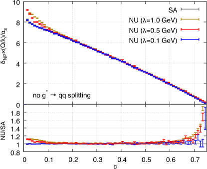
Figure 2: The non-perturbative shift $\delta_{\rm NP}$ for the $C$-parameter defined in Eq. (129), stripped of the $\lambda/Q$ and $\alpha_{s}$ factor, computed with the semi-analytic result of Eq. (129) (labeled SA), and using the numerical implementation of Eq. (163) (labeled NU). The splitting $g^{*}\to q\bar{q}$ is not included. For the numerical calculation, we use $Q=100$ GeV and three different values of $\lambda$.

While the semi-analytic result is linear in $\lambda$ by construction, the numerical one also contains higher powers of $\lambda$ so that the linear term only dominates in the $\lambda\to 0$ limit. This explains the differences between the numerical results obtained with different values of $\lambda$, and also the residual differences between the semi-analytic and numerical results. We also notice that, as we approach the endpoint regions $c=0$ and $c=3/4$, subleading powers of $\lambda$ become more important, thus explaining the larger differences between the semi-analytic and numerical results there. Overall, we observe good agreement between the results obtained with the two methods.

5.4 Comparison with the full large-$n_{f}$ calculation

As a second test of our approach, we compute coefficients of ${\cal O}(\lambda)$ terms for various observables using Eq. (163) and compare them with the result of a full numerical calculation performed in the large-$n_{f}$ approximation. This comparison is shown in Fig. 3 for the differential distributions of the $C$-parameter and the thrust.

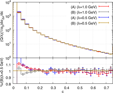
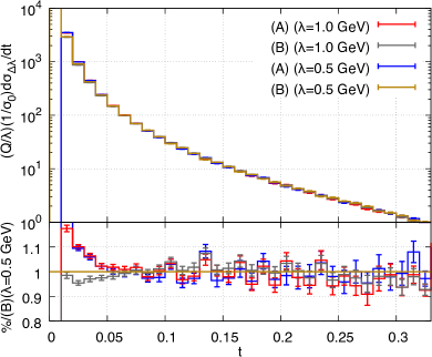
Figure 3: Non-perturbative shift in the differential distributions for the $C$-parameter (left) and the thrust (right), obtained from Eq. (163) (A), and from a full calculation in the large-$n_{f}$ limit (B). Results are shown for the process $\gamma^{*}\to d\bar{d}\gamma$, with $Q=100$ GeV and $\lambda=1$ GeV, $\lambda=0.5$ GeV.

In all cases, we perform the computation for $\lambda=0.5~{}{\rm GeV}$ and $\lambda=1~{}{\rm GeV}$. For the numerical approach based on Eq. (163), we use the mapping (ii) and Eq. (158) for the soft amplitude in the numerical implementation of Eq. (163). Details of the full calculation are reported in Appendix C.

Since the results shown in Fig. 3 are divided by $\lambda$, the agreement between the $\lambda=0.5~{}{\rm GeV}$ and $\lambda=1~{}{\rm GeV}$ cases indicates that the dependence of the observable on $\lambda$ is indeed linear and that Eq. (163) captures the $\lambda$-dependence correctly. For values of the $C$-parameter $c\lesssim 0.15$ and the thrust $t\lesssim 0.07$, the results of the exact calculation performed for two values of $\lambda$ deviate from each other and from the result obtained with the help of Eq. (163). This is an indication of the fact that higher powers of $\lambda$ become important in these regions so that smaller values of $\lambda$ need to be used for these values of $c$ and $t$ to enable the extraction of $\mathcal{O}(\lambda)$ terms from the large-$n_{f}$ computation. Apart from this caveat, Fig. 3 gives strong evidence that one can use Eq. (163) to compute linear power corrections to generic shape variables.

5.5 Non-perturbative correction as a shift in the shape variable

Having verified a simplified method for computing linear power corrections to generic shape observables, we can now use it to derive non-perturbative corrections to them. We will start with a brief overview of the history of such computations.

Non-perturbative corrections to shape variables in the two-jet limit have been considered in Refs. Manohar:1994kq ; Webber:1994cp ; Dokshitzer:1995zt ; Nason:1995np ; Dokshitzer:1995qm ; Dasgupta:1996ki ; Nason:1996pk ; Beneke:1997sr ; Dokshitzer:1997ew ; Dokshitzer:1997iz ; Dokshitzer:1998pt ; Campbell:1998qw ; Luisoni:2020efy (for a review see Ref. Beneke:1998ui ). These non-perturbative corrections are usually employed together with the perturbative ones, as well as with resummations, to extract the strong coupling constant $\alpha_{s}$ from data on $e^{+}e^{-}$ annihilation into hadrons Abbate:2010xh ; Hoang:2015hka ; Catani:1998sf ; Gehrmann:2012sc ; Davison:2009wzs . Non-perturbative corrections are usually fitted in the two-jet region and then extrapolated to the three-jet region, where the value of the strong coupling constant is determined. This approach relies on the assumption that non-perturbative corrections in the three- and two-jet regions are the same.

In a recent paper Luisoni:2020efy , an attempt has been made to gain some insight into the behaviour of these power corrections away from the two-jet limit. The authors of Ref. Luisoni:2020efy studied the $C$-parameter distribution, that, besides the Sudakov region at $c=0$, has a second Sudakov region at $c=3/4$, corresponding to the symmetric three-jets configuration. The presence of this second region allows for a calculation of non-perturbative effects using techniques identical to the ones used for the two-jet region. It was found Luisoni:2020efy that there is significant difference between power corrections in two Sudakov regions. Moreover, it was observed in Ref. Luisoni:2020efy that power corrections in the region where $\alpha_{s}$ is measured strongly depend on the model used to interpolate between the two Sudakov regions. Clearly these results call for a better understanding of the dependence of non-perturbative corrections on the three-jet kinematics.

In the previous sections, we have shown how to compute linear power corrections in the three-jet region in a simplified model with $d\bar{d}\gamma$ final state. Hence, we are in the position to compare our findings in this simplified setup with the approximate results of Ref. Luisoni:2020efy . Conversely, we should be able to reproduce the ratio of non-perturbative corrections in the three-jet symmetric point to the non-perturbative corrections in the two-jet limit obtained in Ref. Luisoni:2020efy ; such a comparison should provide a further test of our numerical approach.

To set up the comparison, we follow the same approach as discussed in Section 4 where it was shown that the non-perturbative corrections to a cumulant of the $C$-parameter can be computed as follows

$$\delta_{\rm NP}(c)=-\frac{{\cal T}_{\lambda}\Sigma(c)}{{\rm d}\sigma(c)/{\rm d}c}.$$ (164)

Although this result was derived in Section 4 for a massive gluon in the final state, it is clear that it also holds if the $g^{*}\to q\bar{q}$ splitting is accounted for.

The non-perturbative correction $\delta_{\rm NP}(c)$ defined in Eq. (164) can be computed directly as a function of $c$ using numerical approach described earlier in this section. However, it is customary to separate it into a normalization factor $h$ that describes non-perturbative corrections in the two-jet region and a $c$-dependent function $\zeta_{q\bar{q}}(c)$ that parametrizes the dependence of non-perturbative corrections on three-jet kinematics. Hence, we write

$$\delta_{\rm NP}(c)=h\zeta_{q\bar{q}}(c).$$ (165)

In principle, the non-perturbative correction in the two-jet region can be computed in the same way as the one in the three-jet region. However, since the two-jet cross section is proportional to $\delta(c)$ in a fixed-order calculation, it is more convenient to relate $h$ with the average value of the $C$-parameter computed in the two-jet region. Indeed, since

$$\frac{{\rm d}\sigma}{{\rm d}c}=\sigma\delta(c+h),$$ (166)

the average value of the $C$-parameter computed for two-jet events is just $-h$. Hence, we can write

$$h=-{\cal T}_{\lambda}\langle C\rangle^{(1)}_{\lambda},$$ (167)

where because of the two-jet constraints the expectation value has to be computed starting from the Born process $\gamma^{*}\to d\bar{d}$.

We compute $h$ numerically for a multitude of different values of $\lambda$; upon linear extrapolation to $\lambda=0$, we obtain

$$h=-9.21(1)\;\left(\frac{\alpha_{s}\lambda}{Q}\right).$$ (168)

This result is consistent with the value $15\pi^{2}/16=9.253$ reported in Ref. Smye:2001gq ; we attribute the differences between numerical and analytic results to higher powers of $\lambda$ that are present in the numerical computation.

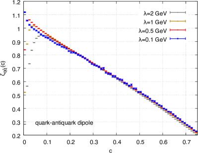
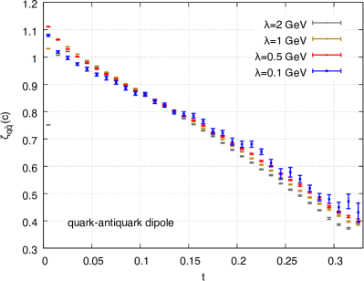
Figure 4: The function $\zeta_{q{\bar{q}}}(c)$ for the $C$-parameter and for thrust $t=1-T$, obtained using $Q=100$ GeV and $\lambda=2$ GeV, $\lambda=1$ GeV, $\lambda=0.5$ GeV and $\lambda=0.1$ GeV. The normalization factor $h$ was taken equal to $-(\lambda/Q)\alpha_{s}\times 15\pi^{2}/16$ for the $C$-parameter, and $-(\lambda/Q)\alpha_{s}\times 5\pi/8$ for thrust.

Having determined the normalization coefficient, we can now turn to the discussion of the function $\zeta_{q{\bar{q}}}$ that parametrizes the dependence of non-perturbative corrections on the $C$-parameter. We plot $\zeta_{q{\bar{q}}}$ in Fig. 4; these results are obtained with $\lambda=2~{}{\rm GeV}$ and $\lambda=1$ GeV. We note that for small values of $C$, $\zeta_{q{\bar{q}}}$ approaches unity. This is explained by the fact that soft emissions factorize independently. So, in the dominant region where both the photon and the gluon are soft, the gluon behaves as if it was radiated by a $q\bar{q}$ dipole (see Appendix D).

Near the three-jet symmetric point, that corresponds to $c=3/4$, we find $\zeta_{q{\bar{q}}}(3/4)=0.226(2)$ for $\lambda=0.1~{}{\rm GeV}$. This value is consistent with the one found in Ref. Luisoni:2020efy , provided that only the radiation of the quark dipole in the abelian limit is considered. We note, however, that since the normalization used here and in Ref. Luisoni:2020efy differ, we can only compare ratios of $\zeta$-functions computed in Luisoni:2020efy ; in what follows we will always consider $\zeta_{\rm LMS}(c)=\zeta(c)/\zeta(0)$ when we quote results of Ref. Luisoni:2020efy . With this clarification, and after setting $C_{A}=0$ in Eq. (18) of Ref. Luisoni:2020efy , we find $\zeta_{\rm LMS}(3/4)=0.224$, consistent with our result.

5.6 Including radiation from the quark-gluon dipoles

The results described so far have been obtained for the $\gamma^{*}\to d{\bar{d}}\gamma$ process and not for the much more interesting case of $\gamma^{*}\to d\bar{d}g$. As we explained in the introduction, this is a well-known limitation of the large-$n_{f}$ approach to computing non-perturbative corrections since processes with gluons at the Born level cannot be dealt with in the theoretical framework employed in this paper.

Although we do not currently know how to overcome this limitation, the structure of the results that we obtained allows us to speculate that, perhaps, it is straightforward to do so. Indeed, our final result shows that linear power corrections to shape variables are captured by the soft approximation to the full matrix element of the $\gamma^{*}\to d\bar{d}\gamma+g$ process. For the cases that we considered so far, the soft approximation originates from a color dipole formed by the $d\bar{d}$ pair. It is tempting to speculate that for the real three-jet production process $\gamma^{*}\to d\bar{d}g$ we can compute linear power corrections by simply considering the emission of an additional soft massive gluon by all the QCD dipoles $d\bar{d}$, $dg$ and $\bar{d}g$ that are present in this case. We emphasize that we cannot prove this statement at this point, but we believe that it provides a reasonable conjecture.

Since the contributions of the three dipoles simply add up, we can write

$$\zeta(x)=\zeta_{q{\bar{q}}}(x)\frac{C_{F}-C_{A}/2}{C_{F}}+\zeta_{qg}(x)\frac{C_{A}}{C_{F}}\,,$$ (169)

where we have exploited the fact that the $dg$ and ${\bar{d}}g$ dipoles contribute equally. We have defined $\zeta_{qg}(x)$ in the same way as $\zeta_{q{\bar{q}}}(x)$ discussed in the previous sub-section, except that we now assume that the radiating dipole is $dg$ (or $\bar{d}g$). We keep, however, the same color factor and the same normalization $h$ used for the $q\bar{q}$ case; hence the $1/C_{F}$ factors in Eq. (169).

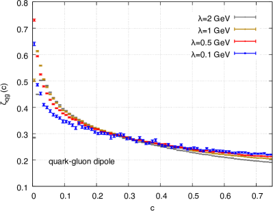
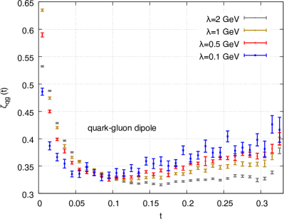
Figure 5: The functions $\zeta_{qg}(c)$ and $\zeta_{qg}(t)$ for the $C$-parameter and for thrust $t=1-T$, obtained using $Q=100$ GeV and $\lambda=2$ GeV, $\lambda=1$ GeV, $\lambda=0.5$ GeV and $\lambda=0.1$ GeV. See text for details.

In Fig. 5 we display the function $\zeta_{qg}$ for the $C$-parameter and the thrust. We observe that in both cases $\zeta_{qg}$ approaches $0.5$ for small $c$ and $t$. This is easily understood, since in this limit $\zeta$ in Eq. (169) should be one by angular ordering arguments and, since $\zeta_{q{\bar{q}}}$ approaches one, it follows that $\zeta_{qg}$ approaches $0.5$ (see Appendix D). In the symmetric three-jet limit $\zeta_{qg}$ approaches the same value as $\zeta_{q{\bar{q}}}$. This is a consequence of the fact that in the symmetric limit the $q{\bar{q}}$ and $qg$ dipoles are geometrically equivalent and, once the color factors are removed, they should give the same results.

We notice that the precision of the numerical result for the $qg$ dipole is inferior to the $q{\bar{q}}$ one and also that near the symmetric point it is worse for thrust than for the $C$-parameter. The first issue is probably related to the fact that the hard emitting gluon is generally softer than the emitting quarks. Thus the effective $Q$ of the emission is smaller in the $qg$ case, leading to larger non-perturbative effects, since they are proportional to $\lambda/Q$. Regarding thrust, we recall that it vanishes in the symmetric three-jet configuration at Born level. This is different for the $C$-parameter, which approaches a constant there.

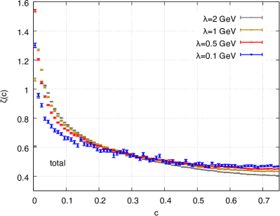
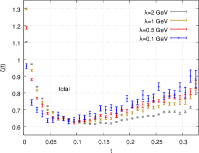
Figure 6: The functions $\zeta(c)$ and $\zeta(t)$ for the $C$-parameter and for thrust $t=1-T$, obtained using $Q=100$ GeV and $\lambda=2$ GeV, $\lambda=1$ GeV, $\lambda=0.5$ GeV and $\lambda=0.1$ GeV. See text for details.

In Fig. 6 we plot $\zeta$ defined in Eq. (169) for the $C$-parameter and for thrust. The results for the $C$-parameter can be compared to Figs. 1 and 3 of Ref. Luisoni:2020efy ; we note again that predictions of Ref. Luisoni:2020efy need to be rescaled so that they assume the value $1$ at $c=0$. The normalized curves agree at the three-jet symmetric point, $c=0.75$, where our result computed for $\lambda=0.1$ is $0.479(5)$, and the (re-scaled) result obtained in Ref. Luisoni:2020efy is $0.476$; the difference can be attributed to terms proportional to $\lambda^{2}$. Among the various extrapolations of the function $\zeta$ presented in Ref. Luisoni:2020efy , their $\zeta_{{\rm b},3}$ curve seems to be the closest to our result.

As a final comment, we notice that for both the $C$-parameter and the thrust, the non-perturbative correction that we computed here is smaller than the one obtained by extrapolating it from the two-jet region to a symmetric point, especially in the case of the $C$-parameter. In Ref. Luisoni:2020efy a fit to $\alpha_{s}$ using the $C$-parameter was given under various assumptions about the shape of the function $\zeta(c)$. For the function $\zeta_{{\rm b},3}$ that, as we said, is closest to our results, the authors of Ref. Luisoni:2020efy extract the value of the strong coupling constant $\alpha_{s}=0.117(3)$. This result is in much better agreement with the world average value $\alpha_{s}=0.118(1)$ as compared to $\alpha_{s}=0.112(2)$ obtained in Ref. Hoang:2015hka using a more conventional treatment of non-perturbative effects. It would be interesting to see if also for the thrust a similar improvement can be achieved.

6 Conclusions

Understanding non-perturbative corrections to collider processes is an interesting problem in theoretical particle physics that received surprisingly little attention in the recent past. However, thanks to the rapid development of the precision physics program at the LHC a case for a better control of non-perturbative effects in hadron collisions becomes stronger.

A possible way to investigate them is to make use of the asymptotic nature of QCD perturbation theory and estimate these effects by studying the ambiguities of a purely perturbative treatment. These ambiguities are related to the infrared pole in the running of the coupling constant. For simple enough processes they can be identified by computing ${\cal O}(\alpha_{s})$ corrections in an abelian version of QCD with a massive gluon, and extracting terms that are non-analytic in $\lambda^{2}$, where $\lambda$ is the gluon mass. From a phenomenological point of view, of particular importance are linear non-perturbative corrections $\mathcal{O}(\Lambda_{\rm QCD}/Q)$. Their presence is exposed by the appearance of $\mathcal{O}(\lambda)$ terms in the massive gluon calculation.

While many explicit computations within the massive gluon framework have been performed in the past, we believe that there is a lack of general understanding of how to approach computations of ${\cal O}(\lambda)$ corrections to a generic scattering process or observable. In a certain sense, this is not surprising since understanding of these $\mathcal{O}(\lambda)$ terms requires a theory of soft effects at next-to-leading power which is more complicated than the familiar soft limit of scattering amplitudes and cross sections.

In this paper, we have shown that it is possible to demonstrate on rather general grounds that many terms that arise at next-to-leading power from the expansions of both phase spaces and matrix elements for typical processes and observables do not produce ${\cal O}(\lambda)$ terms. This result allows us to argue that certain (simplified) collider processes and observables cannot receive linear power corrections. An interesting example of this is the transverse momentum distribution of vector bosons in proton-photon collisions that even if rapidity cuts are applied does not contain $\mathcal{O}(\lambda)$ terms.

We have also shown that an improved understanding of how ${\cal O}(\lambda)$ terms may arise allows us to calculate non-perturbative corrections to shape variables away from Sudakov regions both analytically and numerically. To this end, we have derived a formula that allows us to compute linear power corrections to a generic shape variable in a three-jet configuration. This remarkably simple formula only involves the matrix element of the Born process and soft-radiation eikonal functions of color dipoles. As an application, we have used our formalism to compute non-perturbative corrections to the $C$-parameter and compared it with the result of Ref. Luisoni:2020efy which is based on an interpolation between the two-jet limit ($c=0$) and the three-jet symmetric point ($c=3/4$). As expected, we have found that we can reproduce the results of Ref. Luisoni:2020efy for $c=0$ and $c=3/4$. Between these two points, our results are close to one of the interpolations presented in Ref. Luisoni:2020efy whereas they differ significantly from a few other interpolations provided in that reference. This, of course, is not unexpected since interpolations by their very nature are subject to significant uncertainties.

Our analysis is based on the large-$n_{f}$ approach to the study of non-perturbative corrections; for this reason currently it cannot be applied to processes with gluons at the Born level. It would be interesting to understand how to extend this formalism to deal with these cases as well. Such an extension is, of course, very interesting for hadron collider processes. Also, as we have shown, it may lead to improvements in the description of three-jet events and to more reliable extractions of the strong coupling constant from $e^{+}e^{-}$ data. We look forward to study this interesting problem in the future.

Appendix A Soft integrals

In this appendix, we discuss integrals of the form

$$\vec{I}(v,\tilde{p}_{1,2})=\int[\mathrm{d}k]\theta\left[(k-q)^{2}\right]\frac{(\tilde{p}_{1}\tilde{p}_{2})}{\left(\tilde{p}_{1}k\right)\left(\tilde{p}_{2}k\right)}\left\{1,\frac{(k\,v)}{q^{2}},\frac{\lambda^{2}}{(k\,p_{1,2})}\right\},$$ (170)

where $[\mathrm{d}k]=\mathrm{d}^{4}k\,\delta_{+}(k^{2}-\lambda^{2})/(2\pi)^{3}$ and $v$ is a generic vector, $q=\tilde{p}_{1}+\tilde{p}_{2}$ and $\tilde{p}_{i}^{2}=0$, $i=1,2$. To compute these integrals, in a way that works for all types of dipoles, it is convenient to use Sudakov decomposition. We will discuss the computation for final-final dipole but the calculation can be repeated for initial-final and initial-initial ones with small modifications. We write

$$k=\alpha\,{\tilde{p}}_{1}+\beta\,{\tilde{p}}_{2}+k_{\perp}.$$ (171)

Since $2({\tilde{p}}_{1}{\tilde{p}}_{2})=q^{2}$, we find

$${\rm d}^{4}k\,\delta_{+}(k^{2}-\lambda^{2})\theta\big{[}(q-k)^{2}\big{]}=\frac{q^{2}}{2}{\rm d}\alpha\,{\rm d}\beta\,{\rm d}^{2}\vec{k}_{\perp}\delta(q^{2}\alpha\beta-\vec{k}_{\perp}^{2}-\lambda^{2})\theta\big{[}q^{2}-q^{2}(\alpha+\beta)+\lambda^{2}\big{]},$$ (172)

and

$$2({\tilde{p}}_{1}k)=q^{2}\beta,\;\;\;2({\tilde{p}}_{2}k)=q^{2}\alpha.$$ (173)

When we apply the Sudakov decomposition to all integrals in Eq. (170), we find

$$(v\,k)=({\tilde{p}}_{1}v)\alpha+({\tilde{p}}_{2}v)\beta+(v\,k_{\perp}).$$ (174)

Since this is the only dependence on the $k_{\perp}$-direction that appears in the integrals, the last term in the above equation vanishes after azimuthal integration. Therefore, for the integrals in Eq. (170) the following replacement holds true

$$(v\,k)\to({\tilde{p}}_{1}v)\alpha+({\tilde{p}}_{2}v)\beta.$$ (175)

It follows that to compute Eq. (170) we require the following integrals

$$\frac{1}{16\pi^{2}}\int{\rm d}\alpha\;{\rm d}\beta\;\theta(q^{2}\alpha\beta-\lambda^{2})\theta\big{[}q^{2}(1-\alpha-\beta)+\lambda^{2}\big{]}\frac{1}{\alpha\beta}\left\{1,\alpha,\frac{\lambda^{2}}{\alpha},\frac{\lambda^{2}\beta}{\alpha},\frac{\lambda^{2}\beta^{2}}{\alpha},\frac{\lambda^{4}\beta}{\alpha^{2}}\right\}.$$ (176)

To compute them, we need to know the integration boundaries. They are found from the two $\theta$-functions in the above equation. Suppose that we first integrate over $\beta$. Then,

$$\frac{\lambda^{2}}{q^{2}\alpha}<\beta<1-\alpha+\frac{\lambda^{2}}{q^{2}}.$$ (177)

Boundaries for the subsequent $\alpha$ integration follow from the condition

$$\frac{\lambda^{2}}{q^{2}\alpha}<1-\alpha+\frac{\lambda^{2}}{q^{2}},$$ (178)

which can be re-written as

$$(\alpha-1)\left(\alpha-\frac{\lambda^{2}}{q^{2}}\right)<0.$$ (179)

It follows that the integration interval for $\alpha$ is

$$\frac{\lambda^{2}}{q^{2}}<\alpha<1.$$ (180)

It is then straightforward to see that the various integrals shown in Eq. (170) can be written in terms of the following ones

$$\int\limits_{\lambda^{2}/q^{2}}^{1}\frac{{\rm d}\alpha}{\alpha}\;\int\limits_{\lambda^{2}/(q^{2}\alpha)}^{1-\alpha+\lambda^{2}/q^{2}}\frac{{\rm d}\beta}{\beta}\left\{1,\alpha,\frac{\lambda^{2}}{\alpha},\frac{\lambda^{2}\beta}{\alpha},\frac{\lambda^{2}\beta^{2}}{\alpha},\frac{\lambda^{4}\beta}{\alpha^{2}}\right\}.$$ (181)

This representation makes it completely obvious that the integrals in Eq. (170) are actually functions of $\lambda^{2}$.

Appendix B Computation of the $\mathcal{I}_{i}$ integrals

In this appendix, we compute the integrals

$$\left\{\mathcal{I}_{0},\mathcal{I}_{1},\mathcal{I}_{12}\right\}=\int\limits_{\lambda}^{\omega_{\rm max}}\mathrm{d}\omega\,\beta\times\left\{I_{0},I_{1},I_{12}\right\}$$ (182)

introduced in Section 4, see Eq. (124). The $I_{i}$ integrals are defined in Eq. (122), $\beta=\sqrt{1-\frac{\lambda^{2}}{\omega^{2}}}$ and $\omega_{\rm max}$ is a kinematic bound whose precise form is not important.

We are interested in the small-$\lambda$ expansion of the integrals in Eq. (182). The $\mathcal{I}_{0}$ integral does contain linear terms in $\lambda$. Indeed

$$\mathcal{I}_{0}=\int\limits_{\lambda}^{\omega_{\rm max}}\mathrm{d}\omega\,\beta\,I_{0}=\int\limits_{\lambda}^{\omega_{\rm max}}\mathrm{d}\omega\,\beta=\omega_{\rm max}-\frac{\pi}{2}\lambda+\mathcal{O}(\lambda^{2})$$ (183)

We now study $\mathcal{I}_{1}$. A simple calculation shows that

$$I_{1}=\int\frac{\mathrm{d}\Omega_{k}}{4\pi}\frac{1}{1-\beta\vec{n}\cdot\vec{n}_{1}}=\frac{1}{2\beta}\ln\frac{1+\beta}{1-\beta}.$$ (184)

Integrating by parts, it is then straightforward to obtain

$$\mathcal{I}_{1}=\frac{1}{2}\int\limits_{\lambda}^{\omega_{\rm max}}\mathrm{d}\omega\ln\frac{1+\beta}{1-\beta}=\frac{1}{2}\left[\omega_{\rm max}\ln\frac{\omega_{\rm max}+\sqrt{\omega_{\rm max}^{2}-\lambda^{2}}}{\omega_{\rm max}-\sqrt{\omega_{\rm max}^{2}-\lambda^{2}}}-2\sqrt{w_{\rm max}^{2}-\lambda^{2}}\right],$$ (185)

which implies that for small $\lambda$ the integral $\mathcal{I}_{1}$ can be expanded in powers of $\lambda^{2}$.

To understand whether $\mathcal{I}_{12}$ contains $\mathcal{O}(\lambda)$ terms in the small-$\lambda$ expansion, we need to compute $I_{12}$. To this end, we first combine the two propagators using Feynman parameters

$$I_{12}=\int\limits_{0}^{1}\mathrm{d}x\int\frac{\mathrm{d}\Omega_{k}}{4\pi}\frac{1}{\big{(}1-\beta\vec{n}\cdot\vec{\eta}\big{)}^{2}},$$ (186)

where

$$\eta=x\vec{n}_{1}+(1-x)\vec{n}_{2}.$$ (187)

Choosing the $z$ axis along $\eta$ and integrating over the relative angle we find

$$I_{12}=\int\limits_{0}^{1}\frac{\mathrm{d}x}{1-\beta^{2}\,\vec{\eta}\,^{2}}=\int\limits_{0}^{1}\frac{\mathrm{d}x}{1-\beta^{2}\big{(}1-4x(1-x)s_{12}^{2}\big{)}},$$ (188)

where $s_{12}=\sin(\theta_{12}/2)$. Using the $x\to 1-x$ symmetry of the integrand, it is then easy to obtain

$$I_{12}=\frac{1}{2\beta s_{12}\sqrt{1-\beta^{2}c_{12}^{2}}}\ln\frac{\sqrt{1-\beta^{2}c_{12}^{2}}+\beta s_{12}}{\sqrt{1-\beta^{2}c_{12}^{2}}-\beta s_{12}},$$ (189)

where $c_{12}^{2}=1-s_{12}^{2}=\cos^{2}(\theta_{12}/2)$. We can now investigate the small-$\lambda$ behaviour of $\mathcal{I}_{12}$:

$$\mathcal{I}_{12}=\frac{1}{2s_{12}}\int\limits_{\lambda}^{\omega_{\rm max}}\frac{\mathrm{d}\omega}{\sqrt{1-\beta^{2}c_{12}^{2}}}\ln\frac{\sqrt{1-\beta^{2}c_{12}^{2}}+\beta s_{12}}{\sqrt{1-\beta^{2}c_{12}^{2}}-\beta s_{12}}.$$ (190)

To compute this integral, we change variables $\omega\to\beta$, with

$$\mathrm{d}\omega=\lambda\frac{\beta\mathrm{d}\beta}{(1-\beta^{2})^{3/2}},$$ (191)

and $\beta\to r$ with

$$r=\frac{\beta s_{12}}{\sqrt{1-\beta^{2}c_{12}^{2}}},~{}~{}~{}\mathrm{d}\beta=\frac{s_{12}^{2}\mathrm{d}r}{(c_{12}^{2}r^{2}+s_{12}^{2})^{3/2}}.$$ (192)

We obtain

$$\mathcal{I}_{12}=\frac{\lambda}{2s_{12}^{3}}\int\limits_{0}^{r_{\rm max}}\frac{\mathrm{d}r\,r}{(1-r^{2})^{3/2}}\ln\frac{1+r}{1-r}=\frac{\lambda}{2s_{12}^{3}\sqrt{1-r_{\rm max}^{2}}}\left(\ln\frac{1+r_{\rm max}}{1-r_{\rm max}}-2r_{\rm max}\right),$$ (193)

where $r_{\rm max}=\beta_{\rm max}s_{12}/\sqrt{1-\beta_{\rm max}^{2}c_{12}^{2}}$ and $\beta_{\rm max}=\sqrt{1-\lambda^{2}/w_{\rm max}^{2}}$. It is straightforward to show that the expansion of Eq. (193) in $\lambda$ does not contain $\mathcal{O}(\lambda)$ terms.

Appendix C Full calculation of the shape variables in the large-$n_{f}$ limit

In this appendix we describe computation of QCD corrections to the process $\gamma^{*}\to d\bar{d}+\gamma$ in the large-$n_{f}$ approximation. The exact result of the large-$n_{f}$ calculation can be expressed as FerrarioRavasio:2018ubr

$$\langle O\rangle=\langle O\rangle^{(0)}-\frac{1}{b_{0}\alpha_{s}}\int_{0}^{\infty}\frac{\mathrm{d}\lambda}{\pi}\frac{\mathrm{d}\langle O\rangle^{(1)}_{\lambda}}{d\lambda}\arctan\frac{\pi b_{0}\alpha_{s}}{1+b_{0}\alpha_{s}\log\frac{\lambda^{2}}{\mu_{c}^{2}}},$$ (194)

where $\langle O\rangle_{\lambda}^{(1)}$ is defined in Eq. (137) and

$$\mu_{c}=\mu e^{\frac{5}{6}},~{}~{}~{}b_{0}=-\frac{n_{f}T_{F}}{3\pi}.$$ (195)

By expanding Eq. (194) in $\alpha_{s}$, one obtains a factorial growth associated with a linear renormalon. This leads to an ambiguity of the fully-resummed series corresponding to Eq. (136) (see Appendix A of Ref. FerrarioRavasio:2020guj ).

For the full calculation, we start from Eq. (137). The required amplitudes have been analytically calculated using symbolic manipulation software MAXIMA maxima . The scalar integrals needed for the computation of the virtual corrections have been calculated with the COLLIER library Denner:2016kdg . The virtual contribution is infrared finite, since the gluon mass regulates infrared singularities. We have used dimensional regularization to regularize and extract ultraviolet divergences.

Integration over the phase space of final-state particles in the process $\gamma^{*}\to d\bar{d}\gamma$ diverges in the two-jet limit. To ensure that numerical computations are restricted to a three-jet region, we introduced a suppression factor

$$F_{\rm{supp}}=C^{2},$$ (196)

where $C$ is the $C$-parameter, that vanishes in the two-jet limit regulating the integral. This factor is then divided out when computing distributions and cross sections with cuts. As a result, we are able to obtain correct results as long as we do not attempt to compute observables sensitive to the two-jet region.

The real corrections are obtained by adding the emission of a massive gluon in all possible ways to the Born diagram. Integrating over its momentum, the real emission corrections are affected by collinear divergences, that arise when the photon becomes collinear to one of the primary quarks. These configurations can contribute to the three-jet cross section if the radiated gluon is hard and not collinear. Such singularities are dealt with routinely by the POWHEG-BOX framework Alioli:2010xd , that we adopt for our calculation.

Singularities associated with soft or collinear gluons are regulated by the gluon mass $\lambda$ and manifest themselves as terms proportional to $\log{\lambda}$ raised to second or first power. Similar logarithmic contributions, but with the opposite sign, arise from the virtual corrections, such that the sum of real and virtual corrections is free of $\log\lambda$ terms.

A carefully-constructed importance sampling near the singular regions is needed in order to reliably estimate the $\lambda\to 0$ behaviour. We divide the real contribution into three regions

$$R= R^{(1)}+R^{(2)}+R^{(3)},$$ (197)

where

$$R^{(1)}= \frac{f_{d\gamma}^{2}+f_{\bar{d}\gamma}^{2}}{f_{d\gamma}^{2}+f_{\bar{d}\gamma}^{2}+f_{dg}^{2}+f_{\bar{d}g}^{2}}R,$$ (198)

$$R^{(2)}= \frac{f_{dg}^{2}}{f_{d\gamma}^{2}+f_{\bar{d}\gamma}^{2}+f_{dg}^{2}+f_{\bar{d}g}^{2}}R,$$ (199)

$$R^{(3)}= \frac{f_{\bar{d}g}^{2}}{f_{d\gamma}^{2}+f_{\bar{d}\gamma}^{2}+f_{dg}^{2}+f_{\bar{d}g}^{2}}R,$$ (200)

and

$$f_{ij}=\frac{E_{i}+E_{j}}{(k_{i}+k_{j})^{2}}.$$ (201)

Here, $k_{i}$ and $E_{i}$ denote the four-momentum and the energy of the particle $i$. $R$ is a short-hand notation for the $R^{(\lambda)}_{g^{*}}(\Phi_{3+1})$ appearing in Eq. (139). The different contributions $R^{(i)}$ in Eq. (197) correspond to different kinematic configurations of $d\bar{d}\gamma g$ final state. For example $R^{(1)}$ corresponds to the region where the final state photon becomes collinear to either the $d$ or $\bar{d}$ quark, whereas $R^{(2)}$ and $R^{(3)}$ project on regions where emitted gluon becomes collinear to $d$ and $\bar{d}$, respectively.

The contribution of region (1) is handled in the POWHEG-BOX Alioli:2010xd , which implements the required subtractions of IR singularities associated with configurations containing a soft or a collinear photon. The remaining two regions are finite, but require dedicated importance sampling of the region that becomes singular in the limit $\lambda\to 0$.

Finally, we compute the amplitude for the process $\gamma^{*}\to d\bar{d}\gamma q\bar{q}$. This contribution is IR finite in the $\lambda\to 0$ limit, but is affected by QED singularity associated with the final state photon. We thus proceed as for region (1) case, by evaluating it within the POWHEG-BOX framework. We also computed the process $\gamma^{*}\to d\bar{d}\gamma$ at NLO with a massless gluon and subtracted its result from the $\lambda$-dependent one in order to isolate the linear term.

The shape variable distributions are obtained in a standard way, by computing each contribution to sufficient accuracy so that after the cancellation of $\ln^{2}\lambda$, $\ln\lambda$ and $\lambda^{0}$ terms one can extract the $\lambda$ dependence with enough precision.

Appendix D On the two-jet limit of $C$

In this appendix we elaborate more on the two-jet limit of the cumulant of shape variables within our framework. For simplicity, we focus upon the case of the $C$-parameter, following the calculation of Section 4.

We consider first the process $\gamma^{*}\to q(p_{1})+\bar{q}(p_{2})+\gamma(p_{3})$. Extending the notation of Section 4, we define the “double underlying” Born momenta $\hat{p}_{1}$ and $\hat{p}_{2}$ as follows:

• If ${\tilde{p}}_{3}$ becomes collinear to ${\tilde{p}}_{1}$, then $\hat{p}_{1}\approx{\tilde{p}}_{1}+{\tilde{p}}_{3}$ and $\hat{p}_{2}\approx{\tilde{p}}_{2}$,

• If ${\tilde{p}}_{3}$ becomes collinear to ${\tilde{p}}_{2}$, then $\hat{p}_{2}\approx{\tilde{p}}_{2}+{\tilde{p}}_{3}$ and $\hat{p}_{1}\approx{\tilde{p}}_{1}$,

• If ${\tilde{p}}_{3}$ becomes soft, then $\hat{p}_{2}\approx{\tilde{p}}_{2}$ and $\hat{p}_{1}\approx{\tilde{p}}_{1}$.

We want to show that, in the two-jet limit, the non-perturbative correction of the cumulant of $C$ becomes proportional to the non-perturbative correction to the average value of $C$ in the $\gamma^{*}\to q\bar{q}$ process. Three observations are needed to prove this:

• As $c$ approaches zero, the Born cross section has two collinear-singular regions, when the photon is collinear to either primary quark; a soft singular region, when the photon is soft; and two soft-collinear regions, when the photon is both collinear and soft.

• The correction to the $C$-parameter due to the emission of a soft gluon, i.e. the $C_{k}$ function of Eq. (111), has a smooth limit if any pair of the 1, 2 and 3 particles become collinear, as well as if one of them becomes soft. In particular, if ${\tilde{p}}_{3}$ becomes soft or collinear to either ${\tilde{p}}_{1}$ or ${\tilde{p}}_{2}$ we have

  $$C_{k}(\Phi_{3},k)=-3\sum_{i=1}^{3}\frac{(k{\tilde{p}}_{i})^{2}}{(kq)({\tilde{p}}_{i}q)}\rightarrow-3\sum_{i=1}^{2}\frac{(k\hat{p}_{i})^{2}}{(kq)(\hat{p}_{i}q)}=C_{k}(\Phi_{2},k)$$ (202)

  where we have written collectively $\{{\tilde{p}}_{1},{\tilde{p}}_{2},{\tilde{p}}_{3}\}=\Phi_{3}$ and $\{\hat{p}_{1},\hat{p}_{2}\}=\Phi_{2}$.

• The eikonal factor in Eq. (117) only depends upon the direction of the radiating partons, and not upon the absolute value of their momenta.

For the $q\bar{q}\gamma$ final state, we only have to consider the the case of emission from the quark-antiquark dipole. Our result for the non-perturbative correction, Eq. (129) can be written concisely as

$$\delta_{\rm NP}\equiv-\frac{\mathcal{T}_{\lambda}\Sigma(c)}{{\mathrm{d}\sigma}/{\mathrm{d}C}}=-\frac{\alpha_{s}}{2\pi}C_{F}\times\frac{\int\mathrm{d}\Phi_{3}\delta\big{(}C(\Phi_{3})-c\big{)}|\mathcal{M}(\Phi_{3})|^{2}\,\mathcal{T}_{\lambda}I_{c}(\Phi_{3})}{\int\mathrm{d}\Phi_{3}\delta\big{(}C(\Phi_{3})-c\big{)}|\mathcal{M}(\Phi_{3})|^{2}},$$ (203)

where

$$I_{c}(\Phi_{3};q;\lambda)=8\pi^{2}\int\frac{\mathrm{d}^{4}k}{(2\pi)^{3}}\delta_{+}(k^{2}-\lambda^{2})\theta\big{[}(q-k)^{2}\big{]}\frac{2({\tilde{p}}_{1}{\tilde{p}}_{2})}{({\tilde{p}}_{1}k)({\tilde{p}}_{2}k)}C_{k}(\Phi_{3},k),$$ (204)

and $\mathcal{T}_{\lambda}$ is an operator that takes out the term linear in $\lambda$ from the expression it is applied to. For both the collinear and the soft limits of the Born configuration, the integrand in Eq. (204) becomes

$$\frac{({\tilde{p}}_{1}{\tilde{p}}_{2})}{({\tilde{p}}_{1}k)({\tilde{p}}_{2}k)}C_{k}(\Phi_{3},k)\rightarrow\frac{(\hat{p}_{1}\hat{p}_{2})}{(\hat{p}_{1}k)(\hat{p}_{2}k)}C_{k}(\Phi_{2},k).$$ (205)

Thus, in these limits

$$I_{c}(\Phi_{3};q;\lambda)\rightarrow I_{c}(\Phi_{2};q;\lambda),$$ (206)

that can be taken out of the integrand in Eq. (203), yielding

$$\delta_{\rm NP}\underset{c\to 0}{\approx}-\frac{\alpha_{s}}{2\pi}C_{F}\times\mathcal{T}_{\lambda}I_{c}(\Phi_{2};q;\lambda).$$ (207)

Eq. (207) can be immediately interpreted as the non perturbative correction to the average value of $C$ in the two jet case. Note that $c\to 0$ does not imply that ${\tilde{p}}_{3}$ is either soft or collinear. We could also have ${\tilde{p}}_{1}$ or ${\tilde{p}}_{2}$ soft, or collinear to each other. What is important is that for all dominant singular contributions in the amplitude $I_{c}$ can be taken out of the integral.

We now consider the $\gamma^{*}\to q\bar{q}g$ process, and use the conjecture for non-perturbative corrections that we have described in the text. In comparison to the $\gamma^{*}\to q\bar{q}\gamma$ case, we now have to consider $qg$ dipoles as well. For the $q(p_{1})g(p_{3})$ dipole, the eikonal factor in Eq. (205) becomes

$$\frac{({\tilde{p}}_{1}{\tilde{p}}_{3})}{({\tilde{p}}_{1}k)({\tilde{p}}_{3}k)}C_{k}(\Phi_{3},k).$$ (208)

When ${\tilde{p}}_{2}$ is collinear to ${\tilde{p}}_{3}$, it reduces to

$$\frac{({\tilde{p}}_{1}{\tilde{p}}_{3})}{({\tilde{p}}_{1}k)({\tilde{p}}_{3}k)}C_{k}(\Phi_{3},k)\underset{p_{2}\parallel p_{3}}{\approx}\frac{(\hat{p}_{1}\hat{p}_{2})}{(\hat{p}_{1}k)(\hat{p}_{2}k)}C_{k}(\Phi_{2},k),$$ (209)

as before. However, when ${\tilde{p}}_{1}$ is collinear to ${\tilde{p}}_{3}$ it becomes zero. In this case then

$$\delta_{\rm NP}\underset{c\to 0}{\approx}-\frac{1}{2}\times\frac{\alpha_{s}}{2\pi}C_{F}\times\mathcal{T}_{\lambda}I_{c}(\Phi_{2};q;\lambda).$$ (210)

This result follows because the most enhanced regions when $c\to 0$ are the soft-collinear ones, but only one of the two contributes, hence the factor of one half.

The above reasoning is corroborated by an explicit evaluation of the final result of Section 4, Eq. (128). Setting

$$x_{1}=1-zx_{3},\quad x_{2}=1-(1-z)x_{3}$$ (211)

in that equation, we find that

$${\cal T}_{\lambda}I_{c}\approx-6\pi\left(\frac{\lambda}{\sqrt{q^{2}}}\right)\times 2,$$ (212)

for both the soft $x_{3}\to 0$ and the two collinear $z\to 0$, $z\to 1$ limits. To extend this result to the quark-gluon dipole, we still start from Eq. (128) but assume that 1 and 2 are the quark and the gluon, and 3 is the antiquark. We now use the parametrization

$$x_{1}=1-zx_{2},\quad x_{3}=1-(1-z)x_{2}.$$ (213)

The singular regions of the Born amplitude are then given by $x_{2}\to 0$ and $z\to 0$, $z\to 1$. In this case we find

$${\cal T}_{\lambda}I_{c}\approx-6\pi\left(\frac{\lambda}{\sqrt{q^{2}}}\right)\times\xi,$$ (214)

with $\xi\to 2$ for $z\to 0$, $\xi\to 0$ for $z\to 1$, and $\xi\to 4z^{2}-6z+2$ for $x_{2}\to 0$. Restricting ourself to the most singular regions, i.e. the soft-collinear ones, we see that indeed only one of the two regions contributes, as we have said before.

We further remark that the soft-collinear approximation is enough to get these results, that can thus be considered consequences of angular ordering. In the quark-antiquark dipole case, the result follows also from the full soft factorization that applies in abelian theories. In this case we expect that the limit is reached earlier. This is not the case for the $qg$ dipole, since the Born level gluon and gluon emitted by the $qg$ dipole do not factorize simultaneously in the soft limit.

References

- (1) G. Heinrich, Collider Physics at the Precision Frontier, Phys. Rept. 922 (2021) 1–69, [2009.00516].
- (2) I. I. Y. Bigi, M. A. Shifman, N. G. Uraltsev and A. I. Vainshtein, QCD predictions for lepton spectra in inclusive heavy flavor decays, Phys. Rev. Lett. 71 (1993) 496–499, [hep-ph/9304225].
- (3) M. Beneke, Renormalons, Phys. Rept. 317 (1999) 1–142, [hep-ph/9807443].
- (4) A. V. Manohar and M. B. Wise, Power suppressed corrections to hadronic event shapes, Phys. Lett. B 344 (1995) 407–412, [hep-ph/9406392].
- (5) B. R. Webber, Estimation of power corrections to hadronic event shapes, Phys. Lett. B 339 (1994) 148–150, [hep-ph/9408222].
- (6) R. Akhoury and V. I. Zakharov, On the universality of the leading, 1/Q power corrections in QCD, Phys. Lett. B 357 (1995) 646–652, [hep-ph/9504248].
- (7) Y. L. Dokshitzer and B. R. Webber, Calculation of power corrections to hadronic event shapes, Phys. Lett. B 352 (1995) 451–455, [hep-ph/9504219].
- (8) P. Nason and M. H. Seymour, Infrared renormalons and power suppressed effects in e+ e- jet events, Nucl. Phys. B 454 (1995) 291–312, [hep-ph/9506317].
- (9) Y. L. Dokshitzer, G. Marchesini and B. R. Webber, Dispersive approach to power behaved contributions in QCD hard processes, Nucl. Phys. B 469 (1996) 93–142, [hep-ph/9512336].
- (10) M. Dasgupta and B. R. Webber, Power corrections and renormalons in fragmentation functions, Nucl. Phys. B 484 (1997) 247–264, [hep-ph/9608394].
- (11) M. Beneke, V. M. Braun and L. Magnea, Phenomenology of power corrections in fragmentation processes in e+ e- annihilation, Nucl. Phys. B 497 (1997) 297–333, [hep-ph/9701309].
- (12) Y. L. Dokshitzer and B. R. Webber, Power corrections to event shape distributions, Phys. Lett. B 404 (1997) 321–327, [hep-ph/9704298].
- (13) Y. L. Dokshitzer, A. Lucenti, G. Marchesini and G. P. Salam, Universality of 1/Q corrections to jet-shape observables rescued, Nucl. Phys. B 511 (1998) 396–418, [hep-ph/9707532].
- (14) Y. L. Dokshitzer, A. Lucenti, G. Marchesini and G. P. Salam, On the universality of the Milan factor for 1 / Q power corrections to jet shapes, JHEP 05 (1998) 003, [hep-ph/9802381].
- (15) N. Agarwal, A. Mukhopadhyay, S. Pal and A. Tripathi, Power corrections to event shapes using eikonal dressed gluon exponentiation, JHEP 03 (2021) 155, [2012.06842].
- (16) M. Beneke and V. M. Braun, Heavy quark effective theory beyond perturbation theory: Renormalons, the pole mass and the residual mass term, Nucl. Phys. B 426 (1994) 301–343, [hep-ph/9402364].
- (17) I. I. Y. Bigi, M. A. Shifman, N. G. Uraltsev and A. I. Vainshtein, The Pole mass of the heavy quark. Perturbation theory and beyond, Phys. Rev. D 50 (1994) 2234–2246, [hep-ph/9402360].
- (18) M. Beneke and V. M. Braun, Power corrections and renormalons in Drell-Yan production, Nucl. Phys. B 454 (1995) 253–290, [hep-ph/9506452].
- (19) M. Dasgupta, Power corrections to the differential Drell-Yan cross-section, JHEP 12 (1999) 008, [hep-ph/9911391].
- (20) G. P. Korchemsky, Power corrections in Drell-Yan production beyond the leading order, in 28th International Conference on High-energy Physics, 10, 1996. hep-ph/9610207.
- (21) G. P. Korchemsky and G. F. Sterman, Nonperturbative corrections in resummed cross-sections, Nucl. Phys. B 437 (1995) 415–432, [hep-ph/9411211].
- (22) M. Dasgupta, L. Magnea and G. P. Salam, Non-perturbative QCD effects in jets at hadron colliders, JHEP 02 (2008) 055, [0712.3014].
- (23) S. Ferrario Ravasio, P. Nason and C. Oleari, All-orders behaviour and renormalons in top-mass observables, JHEP 01 (2019) 203, [1810.10931].
- (24) S. Ferrario Ravasio, G. Limatola and P. Nason, Infrared renormalons in kinematic distributions for hadron collider processes, JHEP 06 (2021) 018, [2011.14114].
- (25) G. Luisoni, P. F. Monni and G. P. Salam, -parameter hadronisation in the symmetric 3-jet limit and impact on fits, Eur. Phys. J. C 81 (2021) 158, [2012.00622].
- (26) M. van Beekveld, W. Beenakker, E. Laenen and C. D. White, Next-to-leading power threshold effects for inclusive and exclusive processes with final state jets, JHEP 03 (2020) 106, [1905.08741].
- (27) M. A. Ebert, I. Moult, I. W. Stewart, F. J. Tackmann, G. Vita and H. X. Zhu, Subleading power rapidity divergences and power corrections for qT, JHEP 04 (2019) 123, [1812.08189].
- (28) G. Passarino and M. J. G. Veltman, One Loop Corrections for e+ e- Annihilation Into mu+ mu- in the Weinberg Model, Nucl. Phys. B 160 (1979) 151–207.
- (29) F. E. Low, Bremsstrahlung of very low-energy quanta in elementary particle collisions, Phys. Rev. 110 (1958) 974–977.
- (30) V. B. Berestetskiĭ, E. M. Lifshits, L. P. Pitaevskiĭ, J. B. Sykes and J. S. Bell, Quantum electrodynamics. Landau, L. D., 1908-1968. Teoreticheskaia fizika (Izd. 2-e). English; v. 4. Butterworth-Heinemann, Oxford, 2nd ed. ed., 1982.
- (31) V. Del Duca, N. Deutschmann and S. Lionetti, Momentum mappings for subtractions at higher orders in QCD, JHEP 12 (2019) 129, [1910.01024].
- (32) V. A. Smirnov, Asymptotic expansions of two loop Feynman diagrams in the Sudakov limit, Phys. Lett. B 404 (1997) 101–107, [hep-ph/9703357].
- (33) M. Dasgupta, F. A. Dreyer, K. Hamilton, P. F. Monni, G. P. Salam and G. Soyez, Parton showers beyond leading logarithmic accuracy, Phys. Rev. Lett. 125 (2020) 052002, [2002.11114].
- (34) P. Nason and B. R. Webber, Nonperturbative corrections to heavy quark fragmentation in e+ e- annihilation, Phys. Lett. B 395 (1997) 355–363, [hep-ph/9612353].
- (35) J. M. Campbell, E. W. N. Glover and C. J. Maxwell, Determination of Lambda(QCD) from the measured energy dependence of 1 - thrust, Phys. Rev. Lett. 81 (1998) 1568–1571, [hep-ph/9803254].
- (36) R. Abbate, M. Fickinger, A. H. Hoang, V. Mateu and I. W. Stewart, Thrust at with Power Corrections and a Precision Global Fit for , Phys. Rev. D 83 (2011) 074021, [1006.3080].
- (37) A. H. Hoang, D. W. Kolodrubetz, V. Mateu and I. W. Stewart, Precise determination of from the -parameter distribution, Phys. Rev. D 91 (2015) 094018, [1501.04111].
- (38) S. Catani and B. R. Webber, Resummed C parameter distribution in e+ e- annihilation, Phys. Lett. B 427 (1998) 377–384, [hep-ph/9801350].
- (39) T. Gehrmann, G. Luisoni and P. F. Monni, Power corrections in the dispersive model for a determination of the strong coupling constant from the thrust distribution, Eur. Phys. J. C 73 (2013) 2265, [1210.6945].
- (40) R. A. Davison and B. R. Webber, Non-Perturbative Contribution to the Thrust Distribution in e+ e- Annihilation, Eur. Phys. J. C 59 (2009) 13–25, [0809.3326].
- (41) G. E. Smye, On the 1/Q correction to the C - parameter at two loops, JHEP 05 (2001) 005, [hep-ph/0101323].
- (42) Maxima, Maxima, a Computer Algebra System. Version 5.43.2. http://maxima.sourceforge.net/, 2020.
- (43) A. Denner, S. Dittmaier and L. Hofer, Collier: a fortran-based Complex One-Loop LIbrary in Extended Regularizations, Comput. Phys. Commun. 212 (2017) 220–238, [1604.06792].
- (44) S. Alioli, P. Nason, C. Oleari and E. Re, A general framework for implementing NLO calculations in shower Monte Carlo programs: the POWHEG BOX, JHEP 06 (2010) 043, [1002.2581].