Number of solitons produced from a large initial pulse in the generalized NLS dispersive hydrodynamics theory

Abstract

We show that the number of solitons produced from an arbitrary initial pulse of the simple wave type can be calculated analytically if its evolution is governed by a generalized nonlinear Schrödinger equation provided this number is large enough. The final result generalizes the asymptotic formula derived for completely integrable nonlinear wave equations like the standard NLS equation with the use of the inverse scattering transform method.

I Introduction

It is well known that if a nonlinear wave system supports propagation of solitons with some polarity (bright or dark ones), then a large enough initial pulse with the same polarity evolves at asymptotically large times to a sequence of $N$ separate solitons with some amount of linear radiation. The number $N$ of soliton depends on the initial data and for $N\gg 1$ the energy contained in linear radiation is negligibly small compared with the solitons’ energy in the main approximation with respect to the small parameter $1/N\ll 1$. Consequently, the number of solitons $N$ is one of the most important characteristics of the initial pulse. Besides that, it is relatively easy to measure $N$ experimentally. Thus, the possibility to predict the number of solitons from the initial data is an important task in the theory of nonlinear waves.

If dynamics of the system under consideration is described by a completely integrable wave equation, then the number of solitons is equal to the number of eigenvalues of the associated linear spectral problem (see, e.g., [1, 2]). Consequently, for large number $N\gg 1$ one can apply the quasiclassical WKB method to the linear spectral problem and obtain the asymptotic formula for $N$. For example, in case of the famous KdV equation

$$u_{t}+6uu_{x}+u_{xxx}=0$$ (1)

such a formula was first obtained by Karpman [3] and it reads

$$N\approx\frac{1}{\pi}\int_{-\infty}^{\infty}\sqrt{u_{0}(x)}\,dx,\qquad N\gg 1,$$ (2)

where $u_{0}(x)$ is the initial distribution of the amplitude $u$ and $N$ is the number of eigenvalues of the Schrödinger spectral problem [4, 1, 2] with the “potential” $u_{0}(x)$. A similar formula was derived in Ref. [5] for the NLS equation

$$i\psi_{t}+\frac{1}{2}\psi_{xx}-|\psi|^{2}\psi=0$$ (3)

associated with the Zakharov-Shabat spectral problem [6]. This formula is conveniently formulated in terms of the initial data for the hydrodynamics-like form of Eq. (3) obtained by means of the Madelung substitution

$$\psi(x,t)=\sqrt{\rho(x,t)}\exp(i\phi(x,t)),\qquad\phi_{x}=u(x,t),$$ (4)

so that the NLS equation reduces to the system

$$\begin{split}&\rho_{t}+(\rho u)_{x}=0,\\ &u_{t}+uu_{x}+\rho_{x}+\left(\frac{\rho_{x}^{2}}{8\rho^{2}}-\frac{\rho_{xx}}{4\rho}\right)_{x}=0.\end{split}$$ (5)

In the context of the Gross-Pitaevskii theory [7, 8] of Bose-Einstein condensates of diluted gases, $\rho$ has the meaning of the gas density and $u$ is its flow velocity. This interpretation becomes especially clear in the limit of large pulses with their characteristic size $l\gg 1$. Then the space derivative has the order of magnitude $\partial_{x}\sim l^{-1}\ll 1$ and the last term in the second equation (5) can be neglected. Hence we arrive at equations of Euler hydrodynamics

$$\rho_{t}+(\rho u)_{x}=0,\qquad u_{t}+uu_{x}+\rho_{x}=0$$ (6)

for a compressible fluid with the equation of state $P=\frac{1}{2}\rho^{2}$, where $P$ plays the role of “pressure”.

Dynamics of such a gas is conveniently described with the use of the variables

$$r^{\pm}=\frac{1}{2}u\pm\sqrt{\rho}$$ (7)

called Riemann invariants, so that Eqs. (6) acquire a diagonal form

$$\begin{split}&\frac{\partial r^{+}}{\partial t}+\frac{1}{2}(3r^{+}+r^{-})\frac{\partial r^{+}}{\partial x}=0,\\ &\frac{\partial r^{-}}{\partial t}+\frac{1}{2}(r^{+}+3r^{-})\frac{\partial r^{-}}{\partial x}=0.\end{split}$$ (8)

The Gross-Pitaevskii equation has dark soliton solutions [9] propagating in the form of dips along a uniform background $\rho=\overline{\rho},u=\overline{u}$. If the initial distributions $\overline{\rho}_{0}(x),\overline{u}_{0}(x)$ correspond to a large dip in the density, $0<\overline{\rho}_{0}(x)<\overline{\rho}$ and $\overline{u}_{0}(x)\to 0$ as $|x|\to\infty$, then we can transform them to distributions of the Riemann invariants $r_{0}^{\pm}(x)=\overline{u}_{0}(x)/2\pm\sqrt{\overline{\rho}_{0}(x)}$. The asymptotic formulas for a number of dark solitons moving in the positive or negative direction are given, correspondingly, by the equations [5]

$$N_{\pm}=\frac{1}{\pi}\int_{-\infty}^{\infty}\sqrt{(\pm\overline{r}-r_{0}^{+}(x))(\pm\overline{r}-r_{0}^{-}(x))}\,dx,$$ (9)

where $\overline{r}=\sqrt{\overline{\rho}}$.

Less rigorous simple approach to this problem was suggested in Ref. [10] for the whole AKNS hierarchy [11] associated with $2\times 2$-matrix spectral problem written in an equivalent scalar form [12]. Naturally, in case of Eq. (3) it reproduces Eq. (9) (see Ref. [13]). The approach of Refs. [10, 13] is based on the supposition that the solution of the linear spectral problem (the Baker-Akhiezer function) corresponding to the periodic nonlinear wave keeps its form for slightly modulated waves and can be formally continued to the initial state where it becomes a quasiclassical eigenfunction of the spectral problem.

For not completely integrable equations the associated linear spectral problem does not exist and the above approach becomes impossible. Since the process of formation of solitons from an initially smooth pulse is universal from physical point of view and, generally speaking, it does not depend on the fact whether the wave equation is completely integrable or not, other ideas are necessary. An alternative approach was suggested in Refs. [14, 15] and it was based on the Gurevich-Pitaevskii theory of dispersive shock waves (DSWs). According to this theory, transformation of an initially smooth pulse goes through several stages. In the first stage, the pulse changes its form remaining smooth up to the moment of wave breaking when the dispersionless approximation breaks down due to appearance of infinite space derivatives (“gradient catastrophe”). After the wave breaking moment, the second stage starts during which the pulse in the simplest case consists of two parts—a smooth part for which the dispersionless approximation remains correct, and the DSW part represented by a modulated periodic solution of the nonlinear wave equation under consideration where the modulation parameters obey the Whitham modulation equations [17] (see also review articles [18, 19] for more details). In Whitham approximation, the boundary between the two parts is sharp and it is called the small-amplitude edge of the DSW. At last, in the third asymptotic stage of the pulse’s evolution its smooth part becomes negligibly small and the whole pulse evolves to a sequence of separate solitons. The method of Refs. [14, 15] was based on the assumption that the solution of the Whitham equations at the small-amplitude edge of the DSW can be formally prolonged to the smooth part of the pulse. The necessary parameters of the DSW at its small-amplitude edge can be obtained in the important case of initial simple waves with one of the Riemann invariants constant by El’s method [20]. Although the results of this approach were confirmed in several particular cases by their comparison with the results of numerical solutions, it hardly can be considered as obvious, because the Whitham equations are obtained by averaging over fast nonlinear wave oscillations, whereas there are no any oscillations in the smooth part of the pulse and introduction of their wave vector here looks quite artificial. Therefore other approach based on clearer physical ideas seems very desirable.

Recently a new approach has been suggested in Refs. [19, 21]. It is based on an old remark of Gurevich and Pitaevskii [22] that at the mentioned above second stage of evolution the number $N(t)$ of oscillations (wave crests) inside the DSW part increases with time according to the equation

$$\frac{dN}{dt}=\frac{1}{2\pi}k(v_{g}-v_{ph}),$$ (10)

where $k$ is the wave number and $v_{g},v_{ph}$ are the group and the phase velocities, correspondingly, of the wave at the small-amplitude edge of the DSW. If we denote the background amplitude at this edge as $u$ then the dependence $k=k(u)$ can be found by El’s method and the dependence $t=t(u)$ along the path of the small-amplitude edge can be found by the method of Ref. [23]. As a result, Eq. (10) can be integrated along the path of the small-amplitude edge and in the limit $t\to\infty$ we obtain the total number of crests in the DSW which evolve eventually to separate solitons. As was shown in Refs. [21, 24] for several simple particular cases, this method yields the formulas for the number of solitons coinciding with those derived by the method of Refs. [14, 15], so in these cases the formulas are justified by a more reliable approach.

In this paper, we consider the problem of calculation of the number of solitons produced from a simple-wave type of an initial pulse which evolves according to the generalized NLS (gNLS) equation

$$i\psi_{t}+\frac{1}{2}\psi_{xx}-\frac{1}{p}|\psi|^{2p}\psi=0.$$ (11)

It reduces to the standard NLS equation (3) for $p=1$, but for $p\neq 1$ it is not completely integrable. Various forms of nonlinearity in the gNLS equation are used in nonlinear physics. In particular, the regime $2/3<p<1$ describes the superfluid BEC–Bardeen–Cooper–Schrieffer transition in ultracold Fermi gases [25] and the case $p=2/3$ of the so-called unitary limit has drawn considerable attention (see, e.g., [26] and reference therein). Besides that, Eq. (11) with different values of $p$ are very useful and convenient for the study of various properties of dispersive Euler hydrodynamics [27] since it models both integrable and non-integrable situations amenable to analytical study. Here we show that the formula for the number of solitons can be derived by the direct method of Refs. [19, 21] and this formula can be used in applications and general nonlinear physics investigations.

II Basic formulas

We shall present here the basic formulas necessary for derivation of the expression for the number $N$ of solitons.

II.1 Simple waves

We assume that at the dispersionless stage of evolution before the wave breaking moment the pulse has a form of a simple wave. Actually, this is not a serious restriction imposed on the form of the pulse, since for quite arbitrary initial conditions the dispersionless evolution leads in a natural way to splitting the pulse to two pulses propagating in opposite directions and they both are of the simple wave type. Besides that, simple wave pulses can be created by a proper choice of the initial conditions as it happens, for example, in the flow caused by a unidirectional motion of a piston (see, e.g., [28]).

Equations of the dispersionless approximation for Eq. (11) can be obtained by means of substitution (4) into it, separation of real and imaginary parts and neglecting the dispersive terms with higher order space derivatives. As a result, we obtain the Euler equations

$$\rho_{t}+(\rho u)_{x}=0,\qquad u_{t}+uu_{x}+\rho^{p-1}\rho_{x}=0$$ (12)

corresponding to the equation of state $P=\rho^{p+1}/(p+1)$. It is convenient to define the “sound velocity” variable

$$c=\sqrt{dP/d\rho}=\rho^{p/2}.$$ (13)

Then for the Riemann invariants

$$r_{\pm}=\frac{u}{2}\pm\frac{c}{p}$$ (14)

Eqs. (12) transform to

$$\partial_{t}r_{\pm}+(u\pm c)\partial_{x}r_{\pm}=0,$$ (15)

where the characteristic velocities $v_{\pm}=u\pm c$ have simple physical meaning—they correspond to waves propagating with the sound velocity $c=c(\rho)$ downstream or upstream, correspondingly.

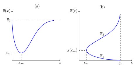
Figure 1: (a) The initial distribution of the local sound velocity $\overline{c}(x)$. (b) The inverse function $\overline{x}(c)$ has two branches $x_{1}(c)$ and $x_{2}(c)$.

In a simple wave one of the Riemann invariants is constant and, to be definite, we assume that $r_{-}=u/2-c/p=-\overline{c}_{0}/p$, where $\overline{c}_{0}$ is the sound velocity far from the localized initial pulse. Then the flow velocity $u(x,t)$ is expressed in terms of the distribution $c(x,t)$ of the local sound velocity,

$$u(x,t)=\frac{2}{p}(c(x,t)-\overline{c}_{0}),$$ (16)

hence $r_{+}=(2c(x,t)-\overline{c}_{0})/p$ and Eq. (15) for $r_{+}$ is transformed to the equation

$$\frac{\partial c}{\partial t}+\frac{1}{p}[(2+p)c-2\overline{c}_{0}]\frac{\partial c}{\partial x}=0.$$ (17)

This is the well known Hopf equation (see, e.g., [29]) and its solution reads

$$x-\frac{1}{p}[(2+p)c-2\overline{c}_{0}]t=\overline{x}(c),$$ (18)

where $\overline{x}(c)$ is the function inverse to the initial distribution $c=\overline{c}(x)$ of the sound velocity (13). We are interested in the initial distributions in the form of localized dips in the uniform state with $c=\overline{c}_{0}$ (see Fig. 1(a)). Hence, the inverse function has two branches $x=\overline{x}_{1,2}(c)$ (see Fig. 1(b)), and each branch gives the solution (18) which defines in implicit form the function $c=c(x,t)$. Evolution of the profile $c=c(x,t)$ leads to wave breaking and, to simplify the notation, we assume that the wave breaking moment corresponds to $t=0$.

II.2 Dispersion relation and El’s equation

After the wave breaking moment a DSW is generated and its small amplitude edge starts its motion along the smooth part of the pulse. Actually, this edge is represented by a linear wave packet propagating with the group velocity of linear waves. The corresponding dispersion relation can be easily found after linearization of Eq. (11) and it can be written in the form (see, e.g., [27])

$$\omega(k,c)=k\left(u\pm\sqrt{c^{2}+k^{2}/4}\right).$$ (19)

The background distribution $c=c(x,t)$ is changing according to the Hopf equation (17) which should be combined with the Hamilton equations

$$\frac{dx}{dt}=\frac{\partial\omega}{\partial k},\qquad\frac{dk}{dt}=-\frac{\partial\omega}{\partial x}$$ (20)

for the packet’s motion. As a simple consequence of these three equations we easily obtain [21] the equation

$$\frac{dk}{dc}=\frac{(\partial\omega/\partial c)_{k}}{u+c-(\partial\omega/\partial k)_{c}}.$$ (21)

This equation was first obtained by El [20] from the small-amplitude limit of the Whitham equations. Its derivation from Hamilton’s equations demonstrates its much wider applicability region. For example, it was applied in Ref. [30] to propagation of localized wave packets along arbitrary large scale smooth simple waves. In case of motion of the small-amplitude edge of a DSW it should be solved with the initial condition

$$k(\overline{c}_{0})=0$$ (22)

which means that the wave breaking occurs at the boundary with the undisturbed region where $c=\overline{c}_{0}$ and in the Whitham approximation the DSW at the initial wave breaking moment shrinks to a point without any oscillations inside.

To solve this equation, it is convenient to introduce the variable [14]

$$\alpha(c)=\sqrt{1+\frac{k^{2}(c)}{4c^{2}}},\qquad k(c)=2c\sqrt{\alpha^{2}(c)-1},$$ (23)

so that Eq. (21) transforms to

$$\frac{d\alpha}{dc}=-\frac{(1+\alpha)(2/p-1+2\alpha)}{c(1+2\alpha)},$$ (24)

which can be easily solved with the initial condition $\alpha(\overline{c}_{0})=1$ to give [27]

$$\frac{c(\alpha)}{\overline{c}_{0}}=\left(\frac{2}{1+\alpha}\right)^{\frac{p}{3p-2}}\left(\frac{2+p}{2-p+2p\alpha}\right)^{\frac{2(p-1)}{3p-2}}.$$ (25)

The function $c=c(\alpha)$ can be inverted in three particular cases [27]:

$$\begin{split}&p=1,\quad\alpha(c)=\frac{2\overline{c}_{0}}{c}-1,\\ &p=2,\quad\alpha(c)=\frac{1}{2}\left(\sqrt{1+8\left(\frac{\overline{c}_{0}}{c}\right)^{2}}-1\right),\\ &p=\frac{1}{2},\quad\alpha(c)=\frac{1}{16}\left(5\sqrt{\frac{\overline{c}_{0}}{c}\left(25\frac{\overline{c}_{0}}{c}-16\right)}+25\frac{\overline{c}_{0}}{c}-24\right).\end{split}$$ (26)

Substitution of these formulas into Eq. (23) yields explicit expressions for the function $k(c)$.

II.3 Path of the small amplitude edge

The small amplitude edge propagates with the group velocity

$$\frac{dx}{dt}=\frac{d\omega}{dk}=\frac{2}{p}(c-\overline{c}_{0})+c(\alpha(c)-\alpha^{-1}(c)).$$ (27)

According to Ref. [23], this equation must be compatible with the solution (18), where $c$ equals to the local value of the sound velocity at the point of location of the wave packet. This condition leads to the linear equation

$$\frac{c(\alpha-1)(2\alpha+1)}{\alpha}\frac{dt}{dc}-\frac{2+p}{p}t=\overline{x}^{\prime}(c),$$ (28)

which should be solved first with the initial condition $t(\overline{c}_{0})=0$. Easy integration yields

$$\begin{split}t=t_{1}(c)&=\frac{1}{\sqrt{c(\alpha(c)-1)}}\left(\frac{\alpha(c)+1}{2-p+2p\alpha(c)}\right)^{\frac{1}{3p-2}}\\ &\times\int_{\overline{c}_{0}}^{c}dc^{\prime}\frac{\overline{x}_{1}(c^{\prime})}{\sqrt{c^{\prime}(\alpha(c^{\prime})-1)}(2\alpha(c^{\prime})+1)}\\ &\times\left(\frac{2-p+2p\alpha(c^{\prime})}{\alpha(c^{\prime})+1}\right)^{\frac{1}{3p-2}}\end{split}$$ (29)

for the motion of the wave packet along the branch $x_{1}(c)$: at the moment $t$ the small-amplitude edge is located at the point with the local value of the sound velocity $c$. The expression (29) is correct up to the moment $t_{m}=t_{1}(c_{m})$ when the edge reaches the point with the minimal value $c_{m}$ of the local sound velocity. It is worth noticing that the dispersionless solution (18) preserves the minimal value $c_{m}$ in the distribution $c=c(x,t)$, so $c_{m}$ does not depend on $t$. For $t>t_{m}$ the edge propagates along the solution (18) corresponding to the second branch $\overline{x}_{2}(c)$. Accordingly, Eq. (28) should be solved with the initial condition $t(c_{m})=t_{m}$ and the solution reads

$$\begin{split}t=t_{2}(c)&=\frac{1}{\sqrt{c(\alpha(c)-1)}}\left(\frac{\alpha(c)+1}{2-p+2p\alpha(c)}\right)^{\frac{1}{3p-2}}\\ &\times\Bigg{\{}\int_{\overline{c}_{0}}^{c_{m}}dc^{\prime}\frac{\overline{x}_{1}(c^{\prime})}{\sqrt{c^{\prime}(\alpha(c^{\prime})-1)}(2\alpha(c^{\prime})+1)}\\ &\times\left(\frac{2-p+2p\alpha(c^{\prime})}{\alpha(c^{\prime})+1}\right)^{\frac{1}{3p-2}}\\ &+\int_{c_{m}}^{c}dc^{\prime}\frac{\overline{x}_{2}(c^{\prime})}{\sqrt{c^{\prime}(\alpha(c^{\prime})-1)}(2\alpha(c^{\prime})+1)}\\ &\times\left(\frac{2-p+2p\alpha(c^{\prime})}{\alpha(c^{\prime})+1}\right)^{\frac{1}{3p-2}}\Bigg{\}}.\end{split}$$ (30)

Substitution of the above two formulas into $x(c)=\overline{x}_{1,2}(c)+\frac{1}{p}[(2+p)c-2\overline{c}_{0}]t_{1,2}(c)$ gives the coordinate of the edge at the moment $t(c)$, but we do not need these expressions here.

III Number of solitons

Integration of formula (10) with the use of the dispersion relation (19) gives the total number of wave crests containing in the DSW,

$$N=\frac{1}{8\pi}\int_{0}^{\infty}\frac{k^{3}}{\sqrt{c^{2}+k^{2}/4}}\,dt,$$ (31)

so our task is to evaluate this integral. To this end we pass to integration over $c$ and substitute (23) for $k=k(c)$,

$$N=\frac{1}{\pi}\int\frac{c^{2}}{\alpha(c)}(\alpha^{2}(c)-1)^{3/2}\frac{dt}{dc}dc.$$ (32)

In fact, this integral consists of two parts: first with integration from $\overline{c}_{0}$ to $c_{m}$ with $t=t_{1}(c)$ and second with integration from $c_{m}$ to $\overline{c}_{0}$ with $t=t_{2}(c)$. The derivative $dt/dc$ can be excluded with the use of Eq. (28) and as a result we obtain

$$\begin{split}N=&\frac{1}{\pi}\int_{\overline{c}_{0}}^{c_{m}}\frac{c(\alpha-1)^{1/2}(\alpha+1)^{3/2}}{2\alpha+1}\\ &\times\left[\frac{2+p}{p}(t_{2}-t_{1})+\overline{x}_{2}-\overline{x}_{1}\right]dc.\end{split}$$ (33)

Integration over $c$ can be replaced by integration over $\alpha$ with help of Eq. (24),

$$\begin{split}N=&\frac{p}{\pi}\int_{1}^{\alpha_{m}}\frac{c^{2}(\alpha)(\alpha^{2}-1)^{1/2}}{2-p+2p\alpha}\\ &\times\left[\frac{2+p}{p}(t_{2}-t_{1})+\Phi_{2}-\Phi_{1}\right]d\alpha,\end{split}$$ (34)

where $\alpha_{m}=\alpha(c_{m})$ and $\Phi(\alpha)\equiv\left.\overline{x}^{\prime}(c)\right|_{c=c(\alpha)}$.

When we substitute here the expressions (29) and (30) for $t_{1}$ and $t_{2}$ as well as Eq. (25) for $c(\alpha)$, we obtain the double integral which can be simplified by integration by parts:

$$\begin{split}&\frac{2+p}{\pi}\int_{1}^{\alpha_{m}}\frac{c^{2}(\alpha)(\alpha^{2}-1)^{1/2}}{2-p+2p\alpha}(t_{2}-t_{1})d\alpha\\ &=\frac{1}{\pi}\int_{c_{m}}^{\overline{c}_{0}}\frac{c\alpha\sqrt{\alpha^{2}-1}(\overline{x}^{\prime}_{2}-\overline{x}^{\prime}_{1})}{2\alpha+1}dc.\end{split}$$ (35)

The remaining terms are transformed to

$$\begin{split}&\frac{p}{\pi}\int_{1}^{\alpha_{m}}\frac{c^{2}(\alpha)(\alpha^{2}-1)^{1/2}}{2-p+2p\alpha}(\Phi_{2}-\Phi_{1})d\alpha\\ &=\frac{1}{\pi}\int_{c_{m}}^{\overline{c}_{0}}\frac{c(\alpha+1)\sqrt{\alpha^{2}-1}(\overline{x}^{\prime}_{2}-\overline{x}^{\prime}_{1})}{2\alpha+1}dc,\end{split}$$ (36)

and the sum of the above two expressions yields

$$N=\frac{1}{\pi}\int_{c_{m}}^{\overline{c}_{0}}c(\alpha^{2}-1)^{1/2}(\overline{x}^{\prime}_{2}-\overline{x}^{\prime}_{1})dc.$$ (37)

At last, we replace integration over the interval $c_{m}\leq c\leq\overline{c}_{0}$ by integration over $x$ and take into account Eq. (23) to obtain the final formula

$$N=\frac{1}{2\pi}\int_{-\infty}^{\infty}k(\overline{c}(x))dx,$$ (38)

where $\overline{c}(x)$ is the initial distribution of the local sound velocity. In this expression the function $k(c)$ is obtained by substitution of the function $\alpha(c)$ into Eq. (23). For example, in case $p=1$ of the standard NLS equation we have for $\alpha(c)$ the first expression in Eq. (30), hence $k(c)=4\sqrt{\overline{c}_{0}(\overline{c}_{0}-c)}$ and Eq. (38) reduces to

$$N=\frac{2}{\pi}\int_{-\infty}^{\infty}\sqrt{\overline{c}_{0}(\overline{c}_{0}-\overline{c}(x))}dx.$$ (39)

This formula coincides with formula (9) for $N_{+}$, since for the simple wave initial conditions we have $r_{-}=-\overline{c}_{0},r_{+}=2\overline{c}(x)-\overline{c}_{0}$.

We have obtained Eq. (38) by direct calculation without artificial introduction of the distribution of wave numbers $k(\overline{c}(x))$ along a smooth initial state, as it was done in Refs. [14, 15]. Thus, our derivation makes the assumption about existence of such a distribution quite plausible (see [21]).

IV Comparison with numerical solutions

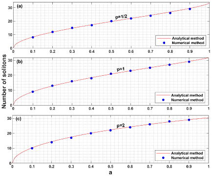
Figure 2: The number of solitons produced from the initial pulse (40) for $l=20$ and different values of $a$. Solid lines correspond to (a) $p=1/2$; (b) $p=1$; and (c) $p=2$ calculated according to the analytical formula (38).

Here we support our analytical theory by comparison of its predictions with the results of numerical solutions of the gNLS equation. We take the initial distribution of the local sound velocity $c=\rho^{p/2}$ in the form

$$\overline{c}(x)=\left[1-\frac{a}{\cosh^{2}(x/l)}\right]^{p/2},$$ (40)

where $a$ denotes the depth of the initial dip in the density distribution and $l$ is its half-length. The initial disturbance must be a simple wave in our approach, so we define the initial distribution of the flow velocity by the formula

$$\overline{u}_{0}(x)=\frac{2}{p}(\overline{c}(x)-\overline{c}_{0}).$$ (41)

Equations (4) allow us to find the initial field $\psi(x,0)$.

In our numerical experiments we choose $l=20$ and change $a$ in the interval $0.1\leq a\leq 0.9$ with the step $\Delta a=0.1$. Such a choice makes the numerical calculations not too time consuming and clearly demonstrates the dependence of the number of solitons on $a$. We have done these calculations for $p=1/2,1$ and 2, when the function $k(\overline{c}(x))$ is given by the explicit formulas (23) and (26). The results of our calculations are presented in Fig. 2. As one can see, the agreement is very good.

V Conclusion

We have shown that the method of calculation of the number of solitons produced from an initial pulse of the simple wave type works very well for the generalized NLS equation having various physical application. The resulting formula (38) has the structure suggested earlier in Ref. [14, 15] on the basis of some suppositions about the properties of solutions of Whitham modulation equations and our derivation makes these suppositions quite plausible. Thus, the developed method and the general formula (38) become a useful tool for predictions of the number of solitons in experiments performed with media whose evolution is described by nonlinear wave equations not belonging to a specific class of completely integrable equations.

- [1] V. E. Zakharov, S. V. Manakov, S. P. Novikov, and L. P. Pitaevskii, The Theory of Solitons: The Inverse Scattering Method, (Nauka, Moscow, 1980) (translation: Consultants Bureau, 1984).
- [2] A. C. Newell, Solitons in Mathematics and Physics, (SIAM, Philadelphia, 1985).
- [3] V. I. Karpman, Phys. Lett. A 25, 708 (1967).
- [4] C. S. Gardner, J. M. Greene, M. D. Kruskal, and R. M. Miura, Phys. Rev. Lett. 19, 1095 (1967).
- [5] S. Jin, C. D. Levermore, D. W. McLaughlin, Comm. Pure Appl. Math., 52, 613 (1999).
- [6] V. E. Zakharov, A. B. Shabat, Zh. Eksp. Teor. Fiz., 64, 1627 (1973) [Sov. Phys. JETP, 37, 823 (1973)].
- [7] E. P. Gross, Nuovo Cimento, 20, 454 (1961).
- [8] L. P. Pitaevskii, Zh. Eksp. Teor. Fiz. 40, 646 (1961) [Sov. Phys. JETP, 13, 451 (1961)].
- [9] T. Tsuzuki, J. Low Temp. Phys. 4, 441 (1971).
- [10] A. M. Kamchatnov, R. A. Kraenkel, B. A. Umarov, Phys. Lett. A 287, 223 (2001).
- [11] M. J. Ablowitz, D. J. Kaup, A. C. Newell, H. Segur, Stud. Appl. Math., 53, 249-315 (1974).
- [12] A. M. Kamchatnov and R. A. Kraenkel, J. Phys. A: Math. Gen. 35, L13 (2002).
- [13] A. M. Kamchatnov, R. A. Kraenkel, B. A. Umarov, Phys. Rev. E 66, 036609 (2002).
- [14] G. A. El, A. Gammal, E. G. Khamis, R. A. Kraenkel, and A. M. Kamchatnov, Phys. Rev. A 76, 053813 (2007).
- [15] G. A. El, R. H. J. Grimshaw, N. F. Smyth, Physica D 237, 2423 (2008).
- [16] A. V. Gurevich, L. P. Pitaevskii, Zh. Eksp. Teor. Fiz. 65, 590 (1973) [Sov. Phys. JETP, 38, 291 (1974)].
- [17] G. B. Whitham, Proc. R. Soc. Lond. A 283, 238 (1965).
- [18] G. A. El, M. A. Hoefer, Physica D 333, 11 (2016).
- [19] A. M. Kamchatnov, Usp. Fiz. Nauk, 191, 52 (2021) [Physics-Uspekhi, 64, 48 (2021)].
- [20] G. A. El, Chaos, 15, 037103 (2005).
- [21] A. M. Kamchatnov, Chaos, 30, 123148 (2020).
- [22] A. V. Gurevich, L. P. Pitaevskii, Zh. Eksp. Teor. Fiz. 93, 871 (1987) [Sov. Phys. JETP, 66, 490 (1987)].
- [23] A. M. Kamchatnov, Phys. Rev. E 99, 012203 (2019).
- [24] A. M. Kamchatnov, Zh. Eksp. Teor. Fiz., 159, 76 (2021) [JETP, 132, 63 (2021)].
- [25] W. Ketterle, M. W. Zwierlein, Riv. Nuovo Cimento, 31, 247 (2008).
- [26] E. A. Kuznetsov, M. Yu. Kagan, and A. V. Turlapov, Phys. Rev. A 101, 043612 (2020).
- [27] M. A. Hoefer, J. Nonlinear Sci. 24, 525 (2014).
- [28] L. D. Landau and E. M. Lifshitz, Fluid Mechanics, (Pergamon, Oxford, 1959).
- [29] G. B. Whitham, Linear and Nonlinear Waves, (Wiley Interscience, New York, 1974).
- [30] A. M. Kamchatnov and D. V. Shaykin, Phys. Fluids, 33, 052120 (2021).