Mixture-Based Correction for Position and Trust Bias in Counterfactual Learning to Rank

Abstract.

In counterfactual learning to rank (CLTR) user interactions are used as a source of supervision. Since user interactions come with bias, an important focus of research in this field lies in developing methods to correct for the bias of interactions. inverse propensity scoring (IPS) is a popular method suitable for correcting position bias. affine correction (AC) is a generalization of IPS that corrects for position bias and trust bias. IPS and AC provably remove bias, conditioned on an accurate estimation of the bias parameters. Estimating the bias parameters, in turn, requires an accurate estimation of the relevance probabilities. This cyclic dependency introduces practical limitations in terms of sensitivity, convergence and efficiency.

We propose a new correction method for position and trust bias in CLTR in which, unlike the existing methods, the correction does not rely on relevance estimation. Our proposed method, mixture-based correction (MBC), is based on the assumption that the distribution of the click-through rates over the items being ranked is a mixture of two distributions: the distribution of click-through rates for relevant items and the distribution of click-through rates for non-relevant items. We prove that our method is unbiased. The validity of our proof is not conditioned on accurate bias parameter estimation. Our experiments show that MBC, when used in different bias settings and accompanied by different learning to rank algorithms, outperforms AC, the state-of-the-art method for correcting position and trust bias, in some settings, while performing on par in other settings. Furthermore, MBC is orders of magnitude more efficient than AC in terms of the training time.

1. Introduction

learning to rank (LTR) is the practice of using supervision to train a ranking function. Traditional LTR methods use explicit relevance labels produced by human annotators (Liu, 2009). In contrast, CLTR uses historical interactions, such as clicks, as labels. Unlike costly manual labels, clicks are available in large amounts for almost no additional cost. The downside of using clicks as relevance labels, however, is bias. Clicks suffer from different types of bias, such as position bias, selection bias, trust bias, etc. (Joachims et al., 2005) As a result of bias, the probability of a click is not the same as the probability of relevance. Thus, in order to use clicks as relevance labels, we should first correct for the bias (Wang et al., 2016; Joachims et al., 2017).

A number of techniques have been proposed to debias clicks and to estimate the probability of relevance based on the probability of clicks. A well-known method is inverse propensity scoring (IPS) (Joachims et al., 2017; Wang et al., 2016), which corrects for the position bias in clicks. IPS relies on the examination hypothesis, i.e., an item is clicked if it is examined and perceived to be relevant by a user. As the name suggests, in IPS clicks are re-weighed by the inverse of the examination probability, a.k.a. propensity. IPS is proved to be unbiased when the clicks suffer from position bias (Joachims et al., 2017). affine correction (AC) generalizes IPS to also correct for trust bias (Vardasbi et al., 2020b). AC has been proved to be unbiased when the clicks suffer from both position and trust bias. The proofs of the unbiasedness of IPS and AC depend on knowledge of the bias parameters. Accurately estimating the bias parameters, in turn, depends on obtaining accurate relevance estimations, which is as hard as the LTR problem itself. In the literature, this cyclic dependency is solved by a regression-based EM (rbEM) algorithm that simultaneously learns the ranker as well as the bias parameters (Wang et al., 2018; Agarwal et al., 2019; Vardasbi et al., 2020b). We argue that integration of a regression function into the standard Expectation-Maximization (EM) leads to a number of practical limitations in terms of (1) sensitivity to the regression function, (2) a lack of guarantees that EM converges to a zero gradient, and (3) low efficiency of the algorithm.

We break the curse of cyclic dependency by proposing a novel debiasing method, mixture-based correction (MBC). Inspired by the idea of score distributions (Arampatzis et al., 2009), we assume that the probability of seeing a specific click-through rate (CTR) for an item at a position in a ranking is a mixture of CTR probabilities for relevant and non-relevant items appearing on that position. More specifically, we assume that an item is clicked if, and only if, one of the following two disjoint events occurs: (1) a user examines the item and the item is actually relevant (i.e., this is a click on a relevant item), or (2) the user examines the item, the item is not relevant, but the user clicks on it anyway due a certain bias, e.g., trust in the search engine (Agarwal et al., 2019) or visual attractiveness of the item (Chen et al., 2012) (i.e., this is a click on a non-relevant item). For each position in a ranking, MBC estimates the distribution of CTRs for these two events and calculates the full distribution of CTRs on that position as their mixture. Then, the probability of relevance for a given item is calculated by Bayes’ rule, as the posterior probability of relevance, given the observed CTR over that item. Finally, the estimated probabilities of relevance are used as labels in a standard LTR algorithm.

We prove that MBC gives an unbiased estimator of the probability of relevance, without any prior knowledge of the bias parameter values. This is a step forward, as IPS and AC do rely on prior knowledge of the bias parameter values to be unbiased. Below, we show theoretically how inaccurate bias parameters prevent AC from completely removing bias.

We confirm our theoretical advances with a set of semi-synthetic experiments. We show that the ranking performance of different LTR algorithms, trained on the relevance estimates of MBC, always converges to the ranking performance where the true relevance labels are available. We also compare MBC with the state-of-the-art correction method for position and trust bias, i.e., AC. We compare them by training LTR algorithms over MBC’s and AC’s respective corrected outputs. We show that in several cases MBC outperforms AC by filling the gap between AC’s ranking performance and the true relevance case. Finally, since both MBC and AC depend to the assumption of a click model to infer and correct for the bias, we conduct robustness experiments in terms of click model mismatch. Specifically, we show that when clicks adhere to the Dependent Click Model (DCM) or the User Browsing Model (UBM), but a different click model, such as the Position-Based Model (PBM), is assumed by the correction methods, MBC is more robust, i.e., its ranking performance is affected less compared to AC.

In summary, the contributions of the paper are:

1. We propose a new debiasing method,  mixture-based correction (MBC), for correcting position and trust bias, and prove its unbiasedness. Our proof is stronger than the unbiasedness proofs for existing methods, as it does not rely on the assumption that the bias parameters are known.

2. We show experimentally that, when used with LTR methods, MBC outperforms AC, the state-of-the-art correction method for position and trust bias, in several settings, while having similar performance in other settings.

3. We show that MBC is orders of magnitude faster than AC, in terms of the training time.

4. We provide experimental evidence that MBC is more robust to click model mismatch compared to AC.

2. Background

The majority of prior work on unbiased LTR, tries to correct for the mismatch between the distribution of clicks and relevance probability due to bias. Bias in clicks means that not all relevant items have the same a priori chance of being clicked. E.g., position bias means that relevant items at the top of a result list usually absorb more clicks than lower ranked relevant items (Joachims et al., 2005); and trust bias means that users trust a search engine and click on higher ranked non-relevant items more than lower ranked items (Agarwal et al., 2019). Usually, these types of bias are modeled with the help of click models (Chuklin et al., 2015).

Below, we review existing methods for correcting position and trust bias. After discussing AC as the state-of-the-art correction method for position and trust bias, we analyze its relevance estimation error and show how inaccurate bias parameters cause AC to remain biased. We also discuss other work related to this paper.

2.1. A review of AC

Agarwal et al. (2019) notice that IPS is still biased when there is also trust bias. In the presence of trust bias, the click probability should be written as follows (for brevity we drop the $(\cdot\mid q,d,k)$ conditions from all the probabilities, where $q$ and $d$ represent the query and item and $k$ is the item position in the results list.):

(1) $$\begin{split}P(C=1)=~{}&P(E=1)\cdot P(R=1)\cdot P(C=1\mid R=1,E=1)\\ ~{}&+P(E=1)\cdot P(R=0)\cdot P(C=1\mid R=0,E=1)\\ =~{}&\alpha P(R=1)+\beta.\end{split}$$

where $C$, $E$ and $R$ indicate click, examination and relevance binary indicators. Vardasbi et al. (2020b) prove that the following correction gives an unbiased estimate of the relevance in this situation:

(2) $$\hat{r}_{q,d}=\frac{c_{q,d,k}-\beta_{q,d,k}}{\alpha_{q,d,k}}.$$

where $c_{q,d,k}$ is the click over document $d$ of query $q$ at position $k$; $\alpha$ and $\beta$ are bias parameters (Eq. 1); and $\hat{r}_{q,d}$ is the estimated relevance of $d$.

2.2. regression-based EM

IPS and AC are unbiased only if the value of the bias parameters such as $\alpha$ and $\beta$ are known, or accurately estimated. Since the standard EM requires the availability of multiple sessions of the same query with different items ordering to work properly (Chapelle and Zhang, 2009), Wang et al. (2018) proposed to use regression-based EM (rbEM) to solve the sparsity problem. In the rbEM, the $P(R=1\mid q,d)$ values obtained in the M-step are first used to fit a regression function, and then, the output of this regression function is used in the next E-step. Though rbEM leads to good results in the CLTR framework with IPS and AC (Agarwal et al., 2019; Vardasbi et al., 2020b; Wang et al., 2018), in this paper we argue that the integration of a regression function into the EM leads to multiple practical limitations, as we explain in Appendix A.1.

2.3. Error analysis of AC

Let us denote the true relevance of document $d$ to query $q$ by $r_{q,d}$, and the probability $P(r_{q,d}=1)$ by $\gamma_{q,d}$. In the presence of trust bias, according to Eq. (1), we have:

(3) $$\mathbb{E}_{c}\left[c_{q,d,k}\right]=\alpha_{q,d,k}\cdot\gamma_{q,d}+\beta_{q,d,k}.$$

In what follows we drop the subscripts for brevity.

Supposing $\alpha^{\prime}$ and $\beta^{\prime}$ are estimates of $\alpha$ and $\beta$ obtained from the rbEM algorithm, AC estimates $r$ as follows:

(4) $$\hat{r}=\frac{c-\beta^{\prime}}{\alpha^{\prime}}.$$

In order to have an unbiased estimator, we need to ensure that $\mathbb{E}_{c}\left[\hat{r}\right]=\mathbb{E}_{r}\left[r\right]$. Therefore, we are interested in $e=\left|\hat{r}-r\right|$. Using Eq. (1), we can calculate the expectation as follows:

(5) $$\begin{split}\mathbb{E}_{c,r}\left[e\right]&=\gamma\left|1-\frac{\alpha+\beta-\beta^{\prime}}{\alpha^{\prime}}\right|+\left(1-\gamma\right)\left|\frac{\beta-\beta^{\prime}}{\alpha^{\prime}}\right|\\ &=\gamma\frac{|\Delta\alpha+\Delta\beta|-|\Delta\beta|}{\alpha^{\prime}}+\frac{|\Delta\beta|}{\alpha^{\prime}},\end{split}$$

where $\Delta\beta=\beta^{\prime}-\beta$ and $\Delta\alpha=\alpha^{\prime}-\alpha$ are estimation errors of the bias parameters. It is important to have the average error converge to zero as the number of sessions associated with the query grows. Eq. (5) shows that only when $\Delta\alpha\rightarrow 0$ and $\Delta\beta\rightarrow 0$, i.e., when the parameter estimations obtained from rbEM are accurate, this is the case. In summary, inaccurate bias parameters estimations cause the AC method to remain biased, even with infinitely many training sessions.

2.4. Mixture of distributions

Our assumption of having a mixture of relevant and non-relevant distributions is related to score distribution models (Arampatzis et al., 2009). But MBC differs in two important ways. First, unlike scores, clicks are feedback and constitute a source of supervision. This makes CLTR used with MBC a supervised learning algorithm as opposed to the unsupervised algorithms based on score distribution models. Second, a score distribution model is built over the corresponding list of items for a single query, whereas our mixture model is built over the items with the same examination probability for different queries. In this sense, our model has a global view over all queries, while the score distribution models have a local view over one query.

2.5. Other related work

Instead of using rbEM, Ai et al. (2018) propose to use the Dual Learning Algorithm (DLA). DLA is shown to be effective in estimating the bias parameters and leading to an unbiased LTR. However, it only models the position bias and it is not clear how it can be extended to work with trust bias.

Qin et al. (2020) use rbEM to estimate the attribute-based propensity, which considers different platforms and feedback sources in addition to the items positions. Dai et al. (2020) define a utility based on the click probability and propose to optimize that utility directly, instead of optimizing retrieval metrics with the hope that they may indirectly improve the CTR. Their approach solves the problem of bias parameter estimation by directly learning a position-aware click model from user interactions.

What our proposed method, MBC, contributes on top of the related work discussed above is that it breaks the cyclic dependency between the bias parameters and relevance probability. This means that in MBC the bias parameters are inferred only using the user interactions, without any direct reliance on the relevance probabilities. In other words, in existing methods relevance estimation is unbiased if the bias parameters are accurately set, and the bias parameters can be set accurately if the relevance estimation is precise. In contrast, with MBC, the correction and bias parameter estimation are performed at the same time, without any reliance on relevance estimation. This enables us to avoid the use of regression functions inside the EM algorithm, which is shown in Appendix A to have practical limitations.

Finally, in (Chandar and Carterette, 2018; Vardasbi et al., 2020a) it is argued that a mismatch between the actual model of clicks and the assumed click model for correction hurts ranking performance of the correction methods. We address this issue by showing that MBC is robust to click model mismatch, specifically, when actual clicks adhere to DCM or UBM while MBC assumes PBM for correction.

3. Mixture-based Correction

In this section, we explain our  mixture-based correction (MBC) method and prove that it gives an unbiased estimate of relevance.

3.1. Method

Our idea is to infer the relevance of an item to a user’s query based on the observed CTR for that query-item pair. Similarly to previous work on CLTR, we assume that user clicks on search results follow the examination hypothesis (Joachims et al., 2017; Ai et al., 2018; Agarwal et al., 2019; Wang et al., 2018; Oosterhuis and de Rijke, 2020; Vardasbi et al., 2020b), that is, a click on an item (or, consequently, the CTR for that item) is affected only by how likely the item is to be examined and perceived relevant by a user. So there are two components, namely, examination and relevance of an item, that contribute to a click on the item. Our goal is to estimate the relevance component.

To rule out the examination component, we consider items with the same examination probability $P(E=1)$. In practice, $P(E=1)$ is not known and one needs a click model to decide which items have the same $P(E=1)$. We will address this issue later in this section. For now, assume that we know which items have the same $P(E=1)$.

For a set of items with the same examination probability $P(E=1)$ there is a certain distribution of CTRs, $P(CTR=x)$. Assuming binary relevance, this distribution has two parts: one for relevant items and one for non-relevant items. So $P(CTR=x)$ can be seen as a mixture of two separate distributions: the distribution $P(CTR=x\mid R=1)$ of CTRs of relevant items and the distribution $P(CTR=x\mid R=0)$ of CTRs of non-relevant items. Formally:

$$P(CTR=x)= \ P(R=1)\cdot P(CTR=x\mid R=1)$$

(6) $${}+\ P(R=0)\cdot P(CTR=x\mid R=0).$$

Now, we can reach our goal and calculate the probability of relevance based on the observed CTR using Bayes’ rule:

(7) $$P(R=1\mid CTR=x)=\frac{P(R=1)\cdot P(CTR=x\mid R=1)}{P(CTR=x)}.$$

These relevance probabilities can ultimately be used for CLTR. Algorithm 1 summarizes the above steps of MBC.

For our MBC method to work, it remains to discuss two things:

Input: click-through rates

Output: Estimates of relevance probability

1 Constitute sets of items with the same $P(E=1)$;

2 forall set of items with the same $P(E=1)$ do

3       Fit a 2-component mixture model to Eq. (3.1);

4       Output the relevance of items according to Eq. (7);

5      

6 end forall

Algorithm 1 mixture-based correction

(1) How to estimate the mixture in Eq. (3.1) (Line 3 in Alg. 1); and (2) How to get items with the same examination probability (Line 1 in Alg. 1).

This is what we turn to next.

Mixture estimation

To infer distributions $P(CTR=x\mid R=i)$ and priors $P(R=i)$ for $i\in\{0,1\}$ in Eq. (3.1), parametric approaches can be used. For example, we can assume a Gaussian or a binomial mixture model. As is common with parametric mixture models, we use standard EM to learn the above distributions and priors (McLachlan and Basford, 1988).

The limitation of the parametric approach to estimating mixtures is that it depends on the choice of the underlying parametric distribution (e.g., Gaussian, binomial, etc). However, in Sec. 3.2, we show that as long as there are enough clicks, the choice of this distribution is not essential to our method. Also, in our experiments in Sec. 5.5, we compare Gaussian and binomial mixture distributions and show that, in practice, both converge to the same performance.

Items with the same examination

The MBC method works on sets of items with the same examination probability. Note that MBC does not require the exact values of examination probabilities, it only requires to know which items have the same examination. To detect the desired sets of items, we propose to use click models (Chuklin et al., 2015).

For instance, we can assume that clicks adhere to the PBM as is common in CLTR (Joachims et al., 2017; Ai et al., 2018; Agarwal et al., 2019; Wang et al., 2018; Oosterhuis and de Rijke, 2020; Vardasbi et al., 2020b). In PBM, all items at the same position in a results list have the same examination probability. And that is all we need from the assumed click model. For cascade models, such as the DCM (Guo et al., 2009) and the UBM (Dupret and Piwowarski, 2008), all items at the same position and with the same pattern of relevant items above them have the same examination probability. In the case of DCM and UBM, the desired set of items can be detected recursively: to collect items with the same examination probability at position $k$, we first use MBC to detect all relevant items at positions above $k$, and then we group items with the same pattern of relevant items above $k$. Note that this recursive process is not cyclic: the grouping of clicks at rank $k$ depends on the reliability of the model at rank $k-1$. Again, no parameter estimation for the assumed click models is required.

Remark 1.

Detecting items with the same examination may seem a bottleneck in real world scenarios. For MBC to work properly, the distributions of relevant and non-relevant CTRs should be separable. This means that the condition of items with the same examination can be loosened by items with almost the same examination. To elaborate, suppose a set of items are considered whose examination probabilities are either $\theta$ or $\theta^{\prime}$. Each examination probability leads to one distribution for relevant CTRs, and one for non-relevant CTRs: there are two relevant CTR distributions and two non-relevant CTR distributions in the set. The relevant (non-relevant) CTR distribution of all the items in the set is itself a mixture of two distributions corresponding to $\theta$ and $\theta^{\prime}$. As long as these two relevant/non-relevant distributions of all items are separable, MBC would be able to distinguish relevant items from non-relevants, and the LTR remains unbiased. This argument is easily extended to cases with more than two different examination probabilities. We will discuss this remark more in Sec. 5.3 and give a toy example for further clarifications.

In the remainder of this section, we prove that the MBC inferred relevance labels are unbiased estimations of the true relevance labels. Consequently, a LTR algorithm trained on these corrected values will be an unbiased LTR.

3.2. Unbiasedness of MBC

In this paper, similar to most previous work on online LTR and CLTR, we assume that clicks on different sessions are independent (Chuklin et al., 2015; Zoghi et al., 2017; Oosterhuis and de Rijke, 2018; Joachims et al., 2017; Ai et al., 2018; Agarwal et al., 2019; Wang et al., 2018; Oosterhuis and de Rijke, 2020; Jagerman et al., 2019; Vardasbi et al., 2020b, a). As discussed in Sec. 3.1, we consider the set of items with almost the same examination probability and fit a mixture model for each such set. We assume that clicking on a relevant item is a random variable with mean $\mu_{1}$ and variance $\sigma^{2}_{1}$. Similarly, clicking on a non-relevant item has mean $\mu_{0}$ and variance $\sigma^{2}_{0}$. For a unique query, repeated in $n$ sessions, assume the clicks over the item $x$ are given by $\{c^{(x)}_{1},c^{(x)}_{2},\ldots,c^{(x)}_{n}\}$. We prove that the CTR defined as

(8) $$v_{x}=\frac{c^{(x)}_{1}+c^{(x)}_{2}+\cdots+c^{(x)}_{n}}{n},$$

can be used to estimate the relevance of $x$, given that $n$ is large enough.

Theorem 3.1.

Assuming independent clicks in different sessions, the clustering of the CTR signal into relevant and non-relevant items converges in probability to the true relevance of the items.

Proof.

Based on the assumptions, the $c^{(x)}_{i}$’s constitute a sequence of independent and identically distributed (i.i.d.) random variables. According to the Central Limit Theorem (CLT), as $n$ grows, $v_{x}$ will converge in probability to $\mathbb{E}_{c}\left[c^{(x)}_{i}\right]$, which is either $\mu_{0}$ or $\mu_{1}$. We are interested in the case where a full recovery of mixture models is possible, i.e., one can fully separate the distribution of relevant CTRs from the distribution of non-relevant CTRs. The variance of $v_{x}$ diminishes linearly by $n$. Consequently, given any threshold value for the variance for which a full recovery is possible, there is a sufficiently large $n$ that leads to the given threshold value. This means that there exists an $n$ such that a full recovery of the mixture components is possible. ∎

We used the Central Limit Theorem for the proof of Theorem 3.1, which does not rely on any specific distribution. In order to get a better understanding of what constitutes a sufficiently large $n$ for full recovery, we discuss the special case of a Gaussian mixture. There is a rich literature on the analysis of the recoverability of Gaussian mixture models (see, e.g., Chen and Yang, 2020). In (Lu and Zhou, 2016) a simple condition is given for almost full recovery of Gaussian mixtures, which translates to the setting of this paper as follows:

(9) $$n=\Omega\left(\left(\frac{\max(\sigma_{0},\sigma_{1})}{\mu_{1}-\mu_{0}}\right)^{2}\right).$$

This means that for any $\mu_{i}$ and $\sigma_{i}$ values, if we increase the number of sessions $n$ so that Eq. (9) holds, the CTR of relevant and non-relevant items can be almost fully separated. In our experiments, where the parameters are set based on previous real-world studies such as (Agarwal et al., 2019), Eq. (9) becomes $n=\Omega(1)$ and we find $n\geq 15$ to be a suitable value based on the convergence of ranking performance.

4. Experimental setup

In this section, we discuss the experimental setup used to demonstrate the effectiveness of our proposed MBC method. Following previous CLTR studies (Joachims et al., 2017; Ai et al., 2018; Jagerman et al., 2019; Agarwal et al., 2019; Oosterhuis and de Rijke, 2020; Vardasbi et al., 2020b), we measure the effectiveness of click debiasing by the ranking performance of LTR when used on top of debiasing methods. Our experiments are performed on two publicly available LTR datasets with query-document features and relevance labels, while clicks are simulated.

4.1. Datasets

As a regular choice in LTR research (Joachims et al., 2017; Ai et al., 2018; Oosterhuis and de Rijke, 2020; Jagerman et al., 2019; Vardasbi et al., 2020b), we use two popular LTR datasets: Yahoo! Webscope (Chapelle and Chang, 2011) and MSLR-WEB30k (Qin and Liu, 2013). For each query, these datasets contain a list of documents with human-generated 5-level relevance labels. Yahoo! has 29 670 queries, 23.84 documents per query on average, and uses 700-feature vectors to represent query-documents; MSLR has 31 339 queries, 120.19 documents per query, and uses 136 features. We use the default provided training, validation and test splits for each dataset. We only use the first fold of MSLR.

4.2. Click simulation

In our experiments, we measure the performance of LTR trained on user clicks. The Yahoo! and MSLR datasets, however, do not contain click information. Following a long line of previous studies (Joachims et al., 2017; Ai et al., 2018; Oosterhuis and de Rijke, 2020; Jagerman et al., 2019; Vardasbi et al., 2020b; Hofmann et al., 2011), we simulate clicks as follows.

Production ranker

First, we simulate a production ranker that is used to create a ranked list of items for each query. Following (Joachims et al., 2017), we train a LTR method on a very small number of randomly selected queries. The intuition is to provide a production ranker that is better than a random ranker, but still has room for improvement. We select 20 random queries from each dataset and use LambdaMART (Burges, 2010) to train a production ranker. To train LambdaMART, we use the LightGBM package (version 3.2.1.99) (Ke et al., 2017) with the following parameters: 300 trees, 31 leaves and a learning rate of $0.05$. Training in this way with 20 queries gives us a decent ranker that performs considerably better than a random ranker, while still having room for improvement. Hence, we can exploit user interactions to improve this production ranker.

The production ranker is then used to rank items for each query. We cut the list of items at top-$m$, as do real-world search engines. We report results for $m=20$. We also performed experiments with the top-$50$, but since the results showed no significant difference compared to the top-$20$, we do not report them in the paper.

User clicks

To simulate clicks, we follow previous studies on trust bias (Agarwal et al., 2019; Vardasbi et al., 2020b). Given a list of items returned by the production ranker for a query $q$, we first compute the click probability for each item $x$ and position $k$ using Eq. (1) and the PBM assumption. (For experiments in Sec. 5.3 we replace PBM with DCM and UBM.) Then, for each item $x$ and position $k$ we simulate a click by sampling from this Bernoulli distribution. Unless stated otherwise, we use $8M$ clicks (with uniformly repeated queries) to train the correction methods. In our experiments, both MBC and AC begin to converge to their final performance after $2M$ clicks. We choose $8M$ to be on the safe side. Eq. (1) depends on two quantities: (1) relevance probabilities; and (2) bias parameters. We will discuss both bellow.

Relevance probabilities

Both datasets used in our experiments provide graded relevance labels. For simulating the clicks in a graded relevance setting, a transformation function is required to change the integer grades into valid relevance probabilities. We employ the following two strategies, assuming $y\in\{0,\ldots,y_{\max}\}$ is the relevance grade:

1. Binarized: Following (Joachims et al., 2017; Vardasbi et al., 2020b) relevance probability can itself be binary: $P(R=1\mid y)=1\quad\text{iff}\quad y>\frac{y_{\max}}{2}$.

2. Graded: The grades can also be turned into probabilities using a linear transformation (Oosterhuis and de Rijke, 2021): $P(R=1\mid y)=\frac{y}{y_{\max}}$.

Bias parameters

Similarly to (Joachims et al., 2017; Ai et al., 2018; Oosterhuis and de Rijke, 2020; Jagerman et al., 2019; Vardasbi et al., 2020b), the position bias for a position $k$ is computed as $P(E=1\mid k)=k^{-\eta}$, where the parameter $\eta$ controls the severity of the position bias. Usually, $\eta=1$ is considered in the CLTR literature (Joachims et al., 2017; Ai et al., 2018; Vardasbi et al., 2020b). In our experiments we consider $\eta\in\{1,2\}$.

For the trust bias, we follow (Vardasbi et al., 2020b) and for each position $k$ compute the parameters as follows:

(10) $$P(C=1\mid R=1,E=1,k) =1-\frac{\min(k,20)+1}{100}$$

(11) $$P(C=1\mid R=0,E=1,k) =\frac{0.65}{\min(k,10)}.$$

4.3. learning to rank

We train a LTR method over the corrected output of different click debiasing methods. In order to show the consistency of our results over different LTR methods, we use two LTR approaches: (1) LambdaMART(Burges, 2010); and (2) DNN, a neural network similar to that of (Vardasbi et al., 2020b). The LambdaMART implementation of LightGBM only works with integer labels, but the input of LTR in our experiments is the relevance probability, which is non-integer. To solve this problem, we made some minor modifications to the source code of LightGBM in order to make it work with non-integer inputs as well. The changed source files are included in the code repository of this paper (see the end of the paper for the link).

4.4. Baselines

We compare the results of MBC to those of AC (Vardasbi et al., 2020b), the state-of-the-art click debiasing method for position and trust bias. We do not include IPS in our comparison, since (1) it cannot correct for trust bias, and (2) ACis a generalization of IPS that leads to the same performance when trust bias is absent (Vardasbi et al., 2020b). In summary, we compare the ranking performance of LTR trained on debiased clicks of our MBC method, with the following settings:

1. Ideal-AC: AC with true bias parameters. This gives the highest potential of AC and is not realistic, since it uses the true values for bias parameters;

2. AC: LTR trained on debiased clicks of AC, using rbEM for propensity estimation (See A.2 for the choice of regression function);

3. No correction: LTR trained on clicks without any debiasing;

4. Relevance probabilities: LTR trained on the true relevance probabilities, obtained from the true relevance labels. This depends on the strategy that is used to transform the integer relevance grades into probabilities (see paragraph Relevance probabilities in Sec. 4.2).

In our experiments, we use the same LTR algorithm for all the methods listed above, so that any differences in ranking performance are solely due to the correction method, and no other factors such as LTR performance.

4.5. Metrics

We measure the ranking performance of different methods by Normalized Discounted Cumulative Gain (NDCG). As we are evaluating using graded relevance datasets, other metrics such as MAP cannot be used. All reported nDCG@10 results are an average of eight independent runs. We use the Student’s t-test to determine significant differences.

5. Results

Our experimental results are centered around three benefits of MBC compared to AC. The first – and most important – benefit is the ranking performance (Sec. 5.2) and efficiency (Sec. 5.4) improvement. The second is its robustness to click model mismatch (Sec. 5.3). The third benefit is that it requires almost no hyper-parameter tuning as opposed to rbEM. Since MBC is based on a standard mixture model, it is free of the so-called hyper-parameters prevalent in deep learning models. On the other hand, rbEM uses a regression function that has a significant impact on the effectiveness and efficiency of the unbiased LTR algorithm (as we show in Appendix A.2).

5.1. An insider’s look into corrected clicks

Before proceeding with the main experimental analysis, we compare the shape of the corrected clicks obtained from MBC and AC. This qualitative analysis is insightful in understanding the intrinsic difference between the two methods.

	Position $1$	Position $9$
Estimated $P(R=1)$	CTR	CTR

Figure 1. Correction comparison of our MBC method with AC in inferring the relevance label from the observed CTR.

Fig. 1 looks into the corrected CTR of MBC and AC. In this figure, the CTR in two different positions of a ranked list are observed. We used the binarized relevance probability (Sec. 4) in this figure for simpler illustration purposes. We see that with enough sessions per query, the relevant and non-relevant items become completely disjoint. Consequently, MBC is able to correctly distinguish between the relevant and non-relevant items and infer their relevance label. The complex transformation of CTRs into relevance labels in MBC allows for accurate estimations of relevance. On the other hand, the linearity of AC leads to wider range of relevance labels, scattered around the true values of zero and one.

Table 1. NDCG@10 comparison of MBC and AC on Yahoo! Webscope and MSLR-WEB30k datasets. Superscripts ^∗ and ^† indicate significance compared to the other correction method with $p<0.01$ and $p<0.1$, respectively.

		Yahoo! Webscope				MSLR-WEB30k
		Normal bias ($\eta=1$)		Severe bias ($\eta=2$)		Normal bias ($\eta=1$)		Severe bias ($\eta=2$)
		Binarized	Graded	Binarized	Graded	Binarized	Graded	Binarized	Graded
LambdaMART	Trained using clicks
	No Correction	0.692	0.691	0.689	0.689	0.400	0.402	0.396	0.397
	AC	0.758	0.763	0.725	0.740	0.426	0.477†	0.337	0.431
	MBC	0.760∗	0.767†	0.753∗	0.748∗	0.428	0.474	0.420∗	0.454∗
	Trained using oracle knowledge
	Ideal-AC	0.758	0.771	0.725	0.740	0.423	0.486	0.337	0.432
	Rel. Probs	0.759	0.774	0.759	0.774	0.429	0.491	0.429	0.491
DNN	Trained using clicks
	No Correction	0.713	0.716	0.710	0.707	0.401	0.415	0.402	0.400
	AC	0.736	0.746∗	0.736	0.746∗	0.404	0.448∗	0.405	0.448∗
	MBC	0.744∗	0.744	0.741∗	0.740	0.406	0.440	0.419∗	0.439
	Trained using oracle knowledge
	Ideal-AC	0.742	0.749	0.737	0.746	0.409	0.451	0.405	0.446
	Rel. Probs	0.743	0.750	0.743	0.750	0.416	0.453	0.416	0.453

5.2. Ranking performance of MBC and AC

In this section, we try to answer the main research question of this paper:

1. How does the MBC method perform compared to AC as the state-of-the-art method for correcting position and trust bias?

In order to determine the effectiveness of methods in debiasing clicks, we measure the ranking performance of a selected LTR algorithm trained over the corrected output of MBC and AC.

Table 1 shows the comparison of MBC and AC in terms of NDCG@10. In this table, we compare the performance for different LTR algorithms: LambdaMART and DNN, and different strategies for transforming relevance grades to probabilities: binarized and graded.

The results show that in most cases MBC performs significantly better than AC. When LambdaMART is used as the LTR algorithm, MBC significantly outperforms AC on both datasets, both binarized and graded settings and both bias severity cases ($\eta=1$ and $\eta=2$), the only exception being the graded MSLR with normal position bias. Things are different for the DNN case. AC significantly outperforms MBC in the graded setting in both datasets. We also see that, with a single correction method, in some settings LambdaMART performs better than DNN, while in others DNN is the winner. Considering the LTR algorithm as a hyperparameter, i.e. for each correction method in each setting, selecting the LTR with the higher ranking performance, we can claim that MBC corrects more effectively than AC, as the best performing MBC leads to better results than the best performing AC. For instance, in graded Yahoo! with severe bias, the best performing AC is obtained from DNN: $0.746$ vs $0.740$, while the best performing MBC is due to LambdaMART: $0.748$ vs $0.740$. We see that LambdaMART MBC outperforms DNN AC in this case.

As can be seen in Table 1, there is a gap between AC (where the bias parameters are estimated using rbEM) and Ideal-AC (where the bias parameters are assumed to be known by an oracle). This shows the dependency of AC on the accuracy of the bias parameters. As a reminder, this dependency is one of our motivations to propose the novel MBC method.

With severe position bias ($\eta=2$), as a result of very low examination probabilities, we observe a noticeable drop in the performance of AC and Ideal-AC in some cases. Specifically, for the binarized MSLR with LambdaMART, we observe that AC performs even worse than the no correction case. This observation underlines the need for variance reduction techniques for the AC method.

Remark 2.

We see that in some of the binarized cases, MBC performs slightly better than the Rel. Probs case, which may seem counterintuitive. The reason is that the evaluation is performed on the graded test set for comparability considerations. As a result, the relevance grades of $\{3,4\}$ as well as $\{0,1,2\}$ are treated the same in the training, but distinguished in evaluation. This is further observable in comparing the Rel. Probs in the binarized and graded settings: the binarized Rel. Probs is not the theoretical upper bound for the ranking performance, the graded Rel. Probs is.

Table 2. NDCG@10 comparison of MBC and AC with PBM assumption on Yahoo! Webscope and MSLR-WEB30k datasets, when cascade models are used for simulating the clicks.

		Yahoo! Webscope				MSLR-WEB30k
		DCM		UBM		DCM		UBM
		Binarized	Graded	Binarized	Graded	Binarized	Graded	Binarized	Graded
LambdaMART	No Correction	0.694	0.691	0.691	0.690	0.405	0.402	0.397	0.400
	AC	0.739	0.753	0.753	0.759	0.411†	0.469	0.387	0.474∗
	MBC	0.752∗	0.760∗	0.756∗	0.763†	0.407	0.477∗	0.410∗	0.469
	Rel. Probs	0.756	0.770	0.756	0.770	0.409	0.485	0.409	0.485
DNN	No Correction	0.709	0.712	0.709	0.716	0.407	0.407	0.391	0.406
	AC	0.728	0.733	0.736	0.743	0.364	0.433	0.402	0.445∗
	MBC	0.741∗	0.743∗	0.741∗	0.742	0.408∗	0.446∗	0.410†	0.441
	Rel. Probs	0.743	0.749	0.743	0.749	0.412	0.453	0.412	0.453

5.3. Click model mismatch

Next, we investigate the effect of a mismatch between a click model that generates clicks and a click model that is used for debiasing:

1. How do MBC and AC methods perform when PBM is assumed for debiasing, whereas user clicks adhere to a different click model?

This is an important question as in reality none of the existing click models can fit user clicks perfectly and there is always a mismatch between a click model that user clicks adhere to and the one that is assumed for debiasing.

In this section, we want to examine the robustness of different correction methods in terms of their assumed click model. Specifically, we simulate clicks based on two well-known models: DCM (Guo et al., 2009), that is a cascade-based click model, and UBM (Dupret and Piwowarski, 2008), that has features of both position-based and cascade-based models. In order to have realistic experiments, we learn the parameters of these click models using the Yandex dataset, which contains a large amount of clicks from a production search engine, and the PyClick library. Since the Yandex dataset has the top-$10$ results, the parameters are obtained for the top-$10$ and our experiments in this section are reported for the top-$10$ setting. Then, we use the learned parameters to simulate clicks similarly to Sec. 4.2, this time using DCM and UBM instead of PBM.

For each case, we debias clicks using MBC and AC with the PBM click model. Table 2 shows the ranking performance of these correction methods.

We observe that MBC always improves over the no correction case, while AC fails to do so in some cases: Binarized UBM with LambdaMART and Binarized DCM with DNN. Furthermore, in most cases, there is a gap between the corrections and the Rel. Probs performance. This gap is due to the mismatch between the actual and assumed click models.

Comparing MBC and AC, we see that MBC outperforms AC in most cases, suggesting that our MBC method is more robust to the click model mismatch. This observation coincides with our expectation, since MBC does not rely on the parameters of click models: as long as the click probabilities over relevant and non-relevant items are separable for each position, MBC with PBM works fine. In other words, unlike AC where the examination probability of each position is estimated by a single value, in MBC different items at the same position are allowed to have different examination probabilities (see Remark 1).

To further illustrate the difference, we give a toy example. Suppose there are two sets of sessions $S_{1}$ and $S_{2}$ such that the true (hidden) examination probability of an item at position $4$ is $0.8$ for sessions in $S_{1}$ and $0.4$ for sessions in $S_{2}$ respectively. Using Eq. 10, the probabilities of click at position $4$ on a relevant item are $0.768$ and $0.384$ and on a non-relevant item are $0.13$ and $0.065$ for sessions in $S_{1}$ and $S_{2}$ respectively. The best AC can do is to estimate the examination probability by the average of $\frac{0.8+0.4}{2}=0.6$, leading to inaccurate relevant probabilities for items in both sets of sessions. MBC, instead, separates the CTRs obtained from sessions. Given enough sessions from each set, a clustering method similar to what we use in MBC, can distinguish between relevant CTRs with mean $\in\{0.768,0.384\}$ and non-relevant CTRs with mean $\in\{0.13,0.065\}$. In other words, as long as the minimum relevant click probability is greater than the maximum non-relevant click probability, MBC manages to separate the two distributions.

5.4. Efficiency of MBC

We measured the running time of MBC and AC on multiple cores of Intel(R) Xeon(R) Gold 5118 CPU @2.30GHz. Here, we only report the time required for correcting clicks, since the LTR part is the same in both MBC and AC. MBC, requires around $110$ seconds to estimate the mixture distributions and correct clicks. Each iteration of the rbEM parameter estimation for AC requires $370$ seconds for fitting the regression function and around $50$ additional seconds to update the bias parameters and target relevance probabilities. The fact that at least 30 iterations are required to get a decent performance of AC (see App. A.2) means that AC requires a minimum of $(370+50)\cdot 30=12600$ seconds to correct clicks. This means that MBC runs approximately $114$ times faster than AC.

Of course, the choice of the regression function plays an important role in the above computations. However, it is worth noting that even with a magical zero-time regression function, AC would still require around $50\cdot 30=1500$ seconds for updating the bias parameters and target relevance probabilities. This hypothetical setting gives a lower bound of around $13$ times for the efficiency superiority of our MBC method over AC.

5.5. MBC with different mixture distributions

MBC relies on mixture models for correcting the clicks. In this section, we will address this question:

1. How do different assumptions for the distribution model of mixture components affect the correction quality?

Particularly, to compare different distribution shapes, we execute two variations of MBC:

1. MBC (Gaussian): A Gaussian (normal) distribution is usually the default choice for modeling real world data, and due to the Central Limit Theorem it is usually a safe choice.

2. MBC (Binomial): We include a Binomial distribution test, since the clicks are usually considered to have a Bernoulli distribution which makes CTR, follow a Binomial distribution.

	nDCG@10
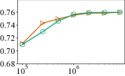
		Number of Training Clicks

Figure 2. Ranking comparison of different mixture distributions for MBC in term of nDCG@10 with respect to different numbers of clicks on Yahoo! Webscope dataset.

Fig. 2 shows the effect of the assumed distribution shape on the performance of MBC. These experiments coincide with the theory provided in Sec. 3. However, we observe that the Gaussian model converges faster than Binomial model. We hypothesize that, since the Binomial model is less generalizable than the Gaussian model, it cannot recover the signal in the presence of high levels of noise in the low data regime.

6. Conclusion

We have proposed a new correction method for position and trust bias, to be used in CLTR, and we have proven its unbiasedness. Our method, mixture-based correction, assumes that the distribution of CTRs of different items is a mixture of two distributions: relevant and non-relevant. Once this mixture is estimated, the relevant items are easily identified and can be used to train a LTR algorithm. Consequently, correction and learning to rank are two separate phases in our MBC method. This breaks the cyclic dependency between bias parameter estimation and relevance inference in existing correction methods. Unlike those methods, in which the unbiasedness relies on accurate bias parameters estimation, the unbiasedness proof of MBC does not rely on knowledge of relevance. This solves some of the practical limitations of the existing methods for correcting position and trust bias which depend on the bias parameter estimation and usually use the rbEM for that.

Particularly, we have found that the cyclic dependency in the existing methods, leads to at least three practical limitations: (1) Severe sensitivity to the choice of the regression function; (2) EM not necessarily converging towards the zero gradient; and, (3) Low efficiency due to repeated use of the regression function. MBC is a new approach that solves all of these limitations as a side benefit.

We have performed extensive semi-synthetic experiments to analyze the strength of MBC at correcting click bias. Our experiments show that MBC outperforms AC, the state-of-the-art correction method for position and trust bias, in most of the settings. Furthermore, we have provided evidence that MBC is more robust to the click model mismatch, compared to AC.

There are several directions that can be followed for the future work: (1) Using non-parametric approaches for estimating the mixtures. (2) Testing on more complex click models than PBM, as MBC is easier to extend to more complex click models than AC.

Code and data

To facilitate the reproducibility of the reported results, this work only made use of publicly available data and our experimental implementation is publicly available at https://github.com/AliVard/MBC.

Appendix A Analysis of regression-based EM

In this Appendix, we list and discuss about three specific practical limitations of rbEM with IPS and AC. As stated earlier, in AC and IPS there is an inherent cyclic dependency between relevance and bias parameters which leads to the use of iterative algorithms like EM. All of the limitations we list here come from the fact that standard EM cannot be used to infer the bias parameters and a regression function has to be used in the middle. Needless to say, these practical limitations do not apply to MBC.

A.1. Practical limitations of rbEM for AC

Sensitivity to the choice of regression function

In rbEM with AC, the regression function is responsible for providing the relevance probabilities in the M-step. This means that the EM is no longer using the values obtained through the likelihood maximization, but an estimate of them obtained from the regression function. Consequently, the performance of EM greatly depends on the performance of the underlying regression function. We show empirically that different choices for the regression function lead to different performances in the ranking of the final unbiased LTR algorithm.

Not necessarily converging to zero gradient

Unlike standard EM, rbEM is not guaranteed to move in the direction of zero gradient. The reason is simple: in the M-step of rbEM, the relevance probabilities that maximize the likelihood function are replaced with the outputs of the regression function, in favor of addressing the otherwise unavoidable sparsity issue. Therefore, the convergence proof of the standard EM, no longer holds for rbEM. Our observations suggest that when using the rbEM, more iterations does not necessarily mean better performance, as opposed to the standard EM.

Low efficiency

The rbEM, by design, requires a regression function to be fitted to the relevance probabilities at each maximization step of the EM algorithm. We have discussed this issue in Sec. 5.4.

A.2. Instability of rbEM for AC

In practice, rbEM is used to estimate the bias parameters for AC. In this set of experiments, we address the following two questions about the performance of rbEM for AC:

1. What is the impact of the choice of regression function for rbEM on the ranking performance of AC?

2. How does the ranking performance of rbEM AC vary as a function of the number of iterations?

Neither of the above questions concern the standard EM, as discussed before. Introducing a regression function in an EM algorithm is a powerful idea to solve the issues of standard EM in CLTR, but it also brings its concerns as well.

We try different regression functions with different loss functions and report the ranking performance on different iterations of rbEM. We use the following regression functions: (1) LambdaMART; and (2) a neural network similar to that of (Vardasbi et al., 2020b). Since the regression function is used for fitting to relevance probabilities, we use the cross entropy loss. Following the literature, we test two cross entropy variations: (1) Sigmoid cross entropy, similar to (Wang et al., 2018; Agarwal et al., 2019); (2) Soft-min-max cross entropy, similar to (Vardasbi et al., 2020b).

	Yahoo! Webscope	MSLR-WEB30k
nDCG@10
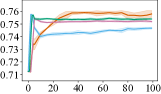
	EM iteration	EM iteration

Figure 3. Regression-based EM ranking performance with different regression functions with respect to EM iterations. Left: Yahoo! Webscope dataset; right: MSLR-WEB30k dataset.

Fig. 3 summarizes the ranking performance of AC with rbEM, with different regression functions, as a function of EM iterations. Based on the observations in this figure, the answers to the questions of this section are: big and a lot. Concerning the first question, we see that different regression functions lead to large differences in ranking performance. More interestingly, the ordering of the regression functions is not preserved in different datasets.

The second question is about the change of the performance as the number of EM iterations increases. Fig. 3 shows that the ranking performance does not always improve with more EM iterations. On the Yahoo! Webscope dataset, the DNN with sigmoid loss has a slight performance drop at iteration 80. On the MSLR-WEB30k dataset, the performance of DNN with sigmoid loss is decreasing between iterations 20 and 50. Another observation relating to the EM iterations are the sudden performance drops at some iterations: DNN with Soft-min-max loss in both datasets. These observations indicate that, unlike the standard EM, the rbEM cannot necessarily be trusted with regard to iterations: The performance is not always increasing with the number of iterations.

Based on the above discussions and according to Fig. 3, our choice for the rbEM baseline for comparison with other methods is as follows: We chose the DNN with sigmoid cross entropy loss function as the regression function. When there are no anomalies, the DNN Sigmoid performs well up until iteration 100. In the cases where there is an anomaly, we use the results of the last iteration before the anomaly.

References

- (1)
- Agarwal et al. (2019) Aman Agarwal, Xuanhui Wang, Cheng Li, Michael Bendersky, and Marc Najork. 2019. Addressing Trust Bias for Unbiased Learning-to-Rank. In The World Wide Web Conference. ACM, 4–14.
- Ai et al. (2018) Qingyao Ai, Keping Bi, Cheng Luo, Jiafeng Guo, and W Bruce Croft. 2018. Unbiased Learning to Rank with Unbiased Propensity Estimation. In The 41st International ACM SIGIR Conference on Research & Development in Information Retrieval. ACM, 385–394.
- Arampatzis et al. (2009) Avi Arampatzis, Stephen Robertson, and Jaap Kamps. 2009. Score Distributions in Information Retrieval. In Advances in Information Retrieval Theory. Springer, 139–151.
- Burges (2010) Christopher J.C. Burges. 2010. From RankNet to LambdaRank to LambdaMART: An Overview. Technical Report MSR-TR-2010-82. Microsoft.
- Chandar and Carterette (2018) Praveen Chandar and Ben Carterette. 2018. Estimating Clickthrough Bias in the Cascade Model. In Proceedings of the 27th ACM International Conference on Information and Knowledge Management. 1587–1590.
- Chapelle and Chang (2011) Olivier Chapelle and Yi Chang. 2011. Yahoo! Learning to Rank Challenge Overview. Journal of Machine Learning Research 14 (2011), 1–24.
- Chapelle and Zhang (2009) Olivier Chapelle and Ya Zhang. 2009. A Dynamic Bayesian Network Click Model for Web Search Ranking. In Proceedings of the 18th International Conference on World Wide Web. ACM, 1–10.
- Chen et al. (2012) Danqi Chen, Weizhu Chen, Haixun Wang, Zheng Chen, and Qiang Yang. 2012. Beyond Ten Blue Links: Enabling User Click Modeling in Federated Web Search. In Proceedings of the Fifth ACM International Conference on Web Search and Data Mining. 463–472.
- Chen and Yang (2020) Xiaohui Chen and Yun Yang. 2020. Cutoff for Exact Recovery of Gaussian Mixture Models. arXiv preprint arXiv:2001.01194 (2020).
- Chuklin et al. (2015) Aleksandr Chuklin, Ilya Markov, and Maarten de Rijke. 2015. Click Models for Web Search. Morgan & Claypool Publishers.
- Dai et al. (2020) Xinyi Dai, Jiawei Hou, Qing Liu, Yunjia Xi, Ruiming Tang, Weinan Zhang, Xiuqiang He, Jun Wang, and Yong Yu. 2020. U-rank: Utility-oriented Learning to Rank with Implicit Feedback. In Proceedings of the 29th ACM International Conference on Information & Knowledge Management.
- Dupret and Piwowarski (2008) Georges E Dupret and Benjamin Piwowarski. 2008. A User Browsing Model to Predict Search Engine Click Data from Past Observations. In Proceedings of the 31st Annual International ACM SIGIR Conference on Research and Development in Information Retrieval. 331–338.
- Guo et al. (2009) Fan Guo, Chao Liu, and Yi Min Wang. 2009. Efficient Multiple-click Models in Web Search. In Proceedings of the Second ACM International Conference on Web Search and Data Mining. ACM, 124–131.
- Hofmann et al. (2011) Katja Hofmann, Shimon Whiteson, and Maarten de Rijke. 2011. Balancing Exploration and Exploitation in Learning to Rank Online. In Advances in Information Retrieval. Springer, 251–263.
- Jagerman et al. (2019) Rolf Jagerman, Harrie Oosterhuis, and Maarten de Rijke. 2019. To Model or to Intervene: A Comparison of Counterfactual and Online Learning to Rank from User Interactions. In Proceedings of the 42nd International ACM SIGIR Conference on Research & Development in Information Retrieval. ACM, 15–24.
- Joachims et al. (2005) Thorsten Joachims, Laura Granka, Bing Pan, Helene Hembrooke, and Geri Gay. 2005. Accurately Interpreting Clickthrough Data as Implicit Feedback. In Proceedings of the 28th Annual International ACM SIGIR Conference on Research and Development in Information Retrieval. ACM, 154–161.
- Joachims et al. (2017) Thorsten Joachims, Adith Swaminathan, and Tobias Schnabel. 2017. Unbiased Learning-to-Rank with Biased Feedback. In Proceedings of the Tenth ACM International Conference on Web Search and Data Mining. ACM, 781–789.
- Ke et al. (2017) Guolin Ke, Qi Meng, Thomas Finley, Taifeng Wang, Wei Chen, Weidong Ma, Qiwei Ye, and Tie-Yan Liu. 2017. LightGBM: A Highly Efficient Gradient Boosting Decision Tree. In Advances in Neural Information Processing Systems. 3146–3154.
- Liu (2009) Tie-Yan Liu. 2009. Learning to Rank for Information Retrieval. Foundations and Trends in Information Retrieval 3, 3 (2009), 225–331.
- Lu and Zhou (2016) Yu Lu and Harrison H Zhou. 2016. Statistical and Computational Guarantees of Lloyd’s Algorithm and its Variants. arXiv preprint arXiv:1612.02099 (2016).
- McLachlan and Basford (1988) Geoffrey J McLachlan and Kaye E Basford. 1988. Mixture models: Inference and applications to clustering. Vol. 38. M. Dekker New York.
- Oosterhuis and de Rijke (2018) Harrie Oosterhuis and Maarten de Rijke. 2018. Differentiable Unbiased Online Learning to Rank. In Proceedings of the 27th ACM International Conference on Information and Knowledge Management. ACM, 1293–1302.
- Oosterhuis and de Rijke (2020) Harrie Oosterhuis and Maarten de Rijke. 2020. Policy-Aware Unbiased Learning to Rank for Top-k Rankings. In Proceedings of the 43rd International ACM SIGIR Conference on Research and Development in Information Retrieval. ACM, 489–498.
- Oosterhuis and de Rijke (2021) Harrie Oosterhuis and Maarten de Rijke. 2021. Unifying Online and Counterfactual Learning to Rank: A Novel Counterfactual Estimator that Effectively Utilizes Online Interventions. In Proceedings of the 14th ACM International Conference on Web Search and Data Mining. ACM, 463–471.
- Qin and Liu (2013) Tao Qin and Tie-Yan Liu. 2013. Introducing LETOR 4.0 datasets. arXiv preprint arXiv:1306.2597 (2013).
- Qin et al. (2020) Zhen Qin, Suming J Chen, Donald Metzler, Yongwoo Noh, Jingzheng Qin, and Xuanhui Wang. 2020. Attribute-based Propensity for Unbiased Learning in Recommender Systems: Algorithm and Case Studies. In Proceedings of the 26th ACM SIGKDD International Conference on Knowledge Discovery & Data Mining. ACM, 2359–2367.
- Vardasbi et al. (2020a) Ali Vardasbi, Maarten de Rijke, and Ilya Markov. 2020a. Cascade Model-based Propensity Estimation for Counterfactual Learning to Rank. In Proceedings of the 43rd International ACM SIGIR Conference on Research and Development in Information Retrieval. ACM, 2089–2092.
- Vardasbi et al. (2020b) Ali Vardasbi, Harrie Oosterhuis, and Maarten de Rijke. 2020b. When Inverse Propensity Scoring does not Work: Affine Corrections for Unbiased Learning to Rank. In Proceedings of the 29th ACM International Conference on Information & Knowledge Management. ACM, 1475–1484.
- Wang et al. (2016) Xuanhui Wang, Michael Bendersky, Donald Metzler, and Marc Najork. 2016. Learning to Rank with Selection Bias in Personal Search. In Proceedings of the 39th International ACM SIGIR conference on Research and Development in Information Retrieval. ACM, 115–124.
- Wang et al. (2018) Xuanhui Wang, Nadav Golbandi, Michael Bendersky, Donald Metzler, and Marc Najork. 2018. Position Bias Estimation for Unbiased Learning to Rank in Personal Search. In Proceedings of the Eleventh ACM International Conference on Web Search and Data Mining. ACM, 610–618.
- Zoghi et al. (2017) Masrour Zoghi, Tomas Tunys, Mohammad Ghavamzadeh, Branislav Kveton, Csaba Szepesvari, and Zheng Wen. 2017. Online Learning to Rank in Stochastic Click Models. arXiv preprint arXiv:1703.02527 (2017).