Renormalization group analysis of Dirac fermions with random mass

Abstract

Two-dimensional (2D) disordered superconductor (SC) in class D exhibits a disorder-induced quantum multicritical phenomenon among diffusive thermal metal (DTM), topological superconductor (TS), and conventional localized (AI) phases. To characterize the quantum tricritical point where these three phases meet, we carry out a two-loop renormalization group (RG) analysis for 2D Dirac fermion with random mass in terms of the $\epsilon$-expansion in the spatial dimension $d=2-\epsilon$. In 2D ($\epsilon=0$), the random mass is marginally irrelevant around a clean-limit fixed point of the gapless Dirac fermion, while there exists an IR unstable fixed point at finite disorder strength that corresponds to the tricritical point. The critical exponent, dynamical exponent, and scaling dimension of the (uniform) mass term are evaluated around the tricritical point by the two-loop RG analysis. Using a mapping between an effective theory for the 2D random-mass Dirac fermion and the (1+1)-dimensional Gross-Neveu model, we further deduce the four-loop evaluation of the critical exponent, and the scaling dimension of the uniform mass around the tricritical point. Both the two-loop and four-loop results suggest that criticalities of a AI-DTM transition line as well as TS-DTM transition line are controlled by other saddle-point fixed point(s) at finite uniform mass.

I Introduction

Low-energy fermionic excitation in $p$-wave superconductors with broken time-reversal and spin-rotational symmetries [1] has a ‘real-valued’ character of its creation being identical to its annihilation (Majorana fermion). Such exotic excitations appear also as low-energy fractionalized magnetic excitations in certain quantum spin models [2], which could be realized in Mott insulators with heavy magnetic ions [3]. Experimental realizations of the Majorana particles acquire a lot of recent interests in condensed matter experiments, while it was suggested that quenched disorders may play crucial role in these experiments [4, 5, 6, 7, 8, 9]. Two-dimensional (2D) class-D disordered superconductor (SC) models [10] are canonical models of Majorana quasiparticles in the presence of the disorder potentials. The class-D disordered SC models have three fundamental phases: topological superconductor (TS) phases with quantized thermal Hall conductance $\kappa_{xy}$ in the unit of $\pi^{2}k^{2}_{B}T/6h$ ($T$ is the temperature, $k_{B}$ is the Boltzmann constant and $h$ is the Plank constant) [11, 12, 13], a diffusive thermal metal (DTM) phase, and conventional Anderson localized (AI) phase with $\kappa_{xy}=0$. Natures of quantum phase transitions among these three fundamental phases have been under active debate for decades, while a number of the numerical studies have been carried out on network models and lattice models [1, 11, 14, 15, 16, 17, 18, 19, 20, 21, 22, 23, 8, 24].

A phase diagram of the class-D disordered SC models has a close connection with a phase diagram of a 2D $\pm J$ random bond Ising model (RBIM). In an exact mapping between the RBIM and disordered fermion models, the diffusive thermal metal phase is absent [1, 25, 14, 16]. Cho and Fisher (CF) [11] found a mapping from the RBIM into a Chalker-Coddington network model (disordered fermion models) [26]. In the phase diagram of the CF network model, all the three fundamental phases appear and a TS-DTM transition line, AI-DTM transition line, and AI-TS transition line meet at a quantum tricritical point. Critical nature of the tricritical point as well as those of the three transition lines have been veiled in mystery. Latest numerical studies of the CF model implies a possibility of an additional fixed-point structure along the AI-TS transition line, which is seemingly related to a Nishimori point in the RBIM [16, 18, 19].

In this paper, we clarify universal scaling properties around the tricritical point (TCP) and the three phase transition lines on the basis of the renormalization group (RG) analysis of 2D Dirac fermion with random Dirac mass. The 2D Dirac fermion is an effective theory for a topological phase transition between two topologically distinct gapped phases in a clean limit, where a change of a uniform Dirac mass term $m$ induces the topological transition. The transition point in the clean limit is described by a 2D gapless Dirac fermion. Any on-site disorder potentials in the 2D gapless Dirac fermion are marginal around the clean-limit fixed point. Particle-hole symmetry in the class D symmetry restricts a form of the disorders to be of the Dirac-mass type. It is known that the Dirac-mass type disorder is marginally irrelevant around the clean-limit fixed point [27]. In this paper, we demonstrate that an infrared (IR) unstable fixed point appears at a finite critical disorder strength, $g=g_{c}$ (Fig. 1), using the two-loop RG analyses and its extension up to the four-loop level. The IR unstable fixed point corresponds to the TCP, where the three phases in the class D systems meet in their phase diagrams. From the clean-limit fixed point to the fixed point at $g=g_{c}$ runs a topological phase transition line, that intervenes between the two gapped phases; AI with $\kappa_{xy}=0$ and TS with $\kappa_{xy}\neq 0$ (Fig. 1). We evaluate a scaling dimension of the uniform Dirac mass and dynamical exponent around the fixed point at $g=g_{c}$ at the two-loop level, and find that the uniform Dirac mass $m$ as well as a deviation of the disorder strength from the critical disorder strength, $\delta g\equiv g-g_{c}$, are relevant scaling variables; Fig. 1. This determines the renormalization group (RG) flow around the TCP as well as the scaling properties of the three transition lines. Namely, the criticality of the TS-AI transition line is controlled by the clean-limit fixed point, while the criticalities of the DTM-TS phase transition and the DTM-AI phase transition are controlled by other theories with finite uniform mass $m$. Using a mapping between an effective model for the random-mass Dirac fermions and Gross-Neveu (GN) model together with preceding four-loop RG calculation of the GN model, we further discuss the scaling dimensions of the uniform mass $m$ and the disorder strength $\delta g$ around the TCP [28, 29, 30]. Both two-loop and four-loop results suggest that the tricritical point (TCP) is unstable in the IR limit (Fig. 1).

The organization of this paper is as follows. In the next section, we introduce two-dimensional (2D) random-mass Dirac fermions as a low-energy theory for Bogoliubov excitations in a disordered $p_{x}+ip_{y}$ superconductor on a lattice. The theory has two controlled parameters; a disorder strength of the random-mass type, and the uniform mass that induces the topological phase transition between two gapped phases with distinct topological numbers. In Sec. III, we introduce an effective low-energy theory for the 2D random-mass Dirac fermions, generalize it in general spatial dimension $d$, and discuss the renormalizability of the effective theory in $d\leq 2$. In Sec. IV, we use minimal subtraction method in $d=2-\epsilon$ and derive two-loop renormalization group (RG) equations for the disorder strength. We obtain an anomalous dimension of the uniform mass as well as the dynamical exponent up to the two-loop level in Sec. IV. In Sec. V, we analyze the RG equation and obtain the critical disorder strength for the TCP, the scaling dimensions of the random mass and dynamical exponent around the TCP. In Sec. VI, we discuss a relation between the effective theory for the 2D random-mass Dirac fermions and (1+1)D SU(N) Gross-Neveu model. The relation gives the four-loop evaluations of the critical disorder strength $g_{c}$ as well as scaling dimensions of the uniform mass $m$ and disorder strength $\delta g$ around the TCP. Sec. VII is devoted to summary and discussion.

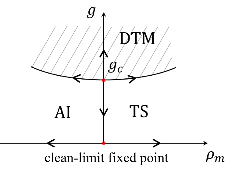
Figure 1: Schematic phase diagram for one-component Dirac fermion with random Dirac mass. DTM is a diffusive thermal metal phase, TS and AI stand a gapped phase with the non-zero topological integer ($C=-1$) and a gapped phase with zero topological integer ($C=0$) respectively. The topological integers in the gapped phases characterize the thermal Hall conductivity as $\kappa_{xy}=C\pi^{2}k^{2}_{B}T/6h$. The vertical axis $g$ represents the disorder strength of the Dirac-mass type and the horizontal axis represents the uniform Dirac mass $m$; $\rho_{m}$ is a dimensionless renormalized mass. A critical point ($g=g_{c}$) at $\rho_{m}=0$ is a tricritical point. The arrow stands for the renormalization group (RG) flow determined by the two-loop and four-loop RG analyses.

II Tight-binding model of spinless $p_{x}+ip_{y}$ superconductor

A square-lattice model of spinless fermions with $p_{x}+ip_{y}$ Cooper pairing and the random chemical-potential type disorder is considered  [31, 32],

$$\mathcal{H}/2= \sum_{\bm{j}}\big{(}\varepsilon_{\bm{j}}+\mu\big{)}\hat{c}_{\bm{j}}^{\dagger}\hat{c}_{\bm{j}}+t\sum_{\bm{j},\mu=x,y}\big{[}\hat{c}_{\bm{j}+\bm{e}_{\mu}}^{\dagger}\hat{c}_{\bm{j}}+\text{h.c.}\big{]}$$

$$+ \Delta\sum_{\bm{j}}\big{[}i\hat{c}_{\bm{j}+\bm{e}_{x}}^{\dagger}\hat{c}_{\bm{j}}^{\dagger}+\hat{c}_{\bm{j}+\bm{e}_{y}}^{\dagger}\hat{c}_{\bm{j}}^{\dagger}+\text{h.c.}\big{]},$$ (1)

with uniform chemical potential $\mu$, nearest-neighbor hopping amplitude $t$ and superconducting pairing amplitude $\Delta\in\mathbb{R}$. Here $\bm{j}\equiv(j_{x},j_{y})$ denotes the lattice vectors, and $\bm{e}_{x}$ and $\bm{e}_{y}$ are primitive unit vectors in $x$ and $y$ direction, respectively. $\varepsilon_{\bm{j}}\in[-W/2,W/2]$ is a short-ranged on-site chemical-potential-type random potential,

$$\langle{\varepsilon_{\bm{i}}\rangle_{\text{dis}}}=0,\quad\langle{\varepsilon_{\bm{i}}\varepsilon_{\bm{j}}\rangle_{\text{dis}}}=\delta_{\bm{i},\bm{j}}W^{2}/2,$$ (2)

where $\langle\cdots\rangle_{\text{dis}}$ stands for Gaussian disorder average. $W$ represents the disorder strength of the random potential. With a two-components Nambu vector,

$$\Psi_{\bm{j}}=\begin{pmatrix}\hat{c}_{\bm{j}}\\ \hat{c}_{\bm{j}}^{\dagger}\end{pmatrix},\quad\Psi_{\bm{j}}^{\dagger}=\begin{pmatrix}\hat{c}_{\bm{j}}^{\dagger}&\hat{c}_{\bm{j}}\end{pmatrix},$$ (3)

the Hamiltonian in Eq. (1) is written as a Bogoliubov-de Gennes (BdG) form,

$$\mathcal{H}=\sum_{\bm{j}}\Psi_{\bm{j}}^{\dagger}\big{[}\mathbb{H}\big{]}_{\bm{j},\bm{m}}\Psi_{\bm{m}}=\sum_{\bm{j}}\Psi_{\bm{j}}^{\dagger}\big{[}\big{(}\varepsilon_{\bm{j}}+\mu\big{)}\sigma_{3}\big{]}\Psi_{\bm{j}}$$

$$+t\!\ \sum_{\bm{j}}\sum_{\mu=x,y}\big{[}\Psi_{\bm{j}+\bm{e}_{\mu}}^{\dagger}\big{(}\sigma_{3}\big{)}\Psi_{\bm{j}}+\mathrm{h.c.}\big{]}$$

$$+i\Delta\!\ \sum_{\bm{j}}\big{[}\Psi_{\bm{j}+\bm{e}_{x}}^{\dagger}\big{(}\sigma_{1}\big{)}\Psi_{\bm{j}}+\Psi_{\bm{j}+\bm{e}_{y}}^{\dagger}\big{(}\sigma_{2}\big{)}\Psi_{\bm{j}}+\mathrm{h.c.}\big{]}$$ (4)

with the three Pauli matrices $\sigma_{i}\,(i=1,2,3)$. The BdG Hamiltonian in Eq. (4) satisfies a particle-hole symmetry,

$$\mathbb{C}\mathbb{H}^{\rm T}\mathbb{C}^{-1}=-\mathbb{H},$$ (5)

with $[\mathbb{C}]_{{\bm{j}},{\bm{m}}}=\delta_{{\bm{j}},{\bm{m}}}\sigma_{1}$. The Hamiltonian also breaks the time-reversal symmetry. The Hamiltonian belongs to the class D in the 10-fold AZ symmetry class classification [10].

The quasi-particle (Bogoliubov) excitation is a gapped excitation, except for $\mu=0,\pm 4t$. At $\mu=0,\pm 4t$, the Bogoliubov excitation forms point nodes at high symmetric momentum points. Especially, when $\mu=-4t$, the particle and the hole bands form a gapless Dirac-cone dispersion around $(k_{x},k_{y})=(0,0)$,

$$\mathbb{H}(\bm{k})\simeq \begin{pmatrix}m-t(k_{x}^{2}+k_{y}^{2})&2\Delta(k_{x}-ik_{y})\\ 2\Delta(k_{x}+ik_{y})&-m+t(k_{x}^{2}+k_{y}^{2})\end{pmatrix}.$$ (6)

A finite $m\equiv\mu+4t$ endows the gapless Dirac fermion with a finite gap. In the gapped phase, the bulk state is characterized by a quantized thermal Hall conductivity $\kappa_{xy}=C\pi^{2}k^{2}_{B}T/6h$ with $C$ a quantized integer number [12]. The gapless point $m=0$ separates the two gapped phases with the quantized number $C=0$ ($m<0$) and $C=-1$ ($m>0$). The low-energy effective theory around $m\simeq 0$ and around the $\Gamma$ point ($\bm{k}\simeq 0$) is described by a Dirac fermion Hamiltonian for a slowly-varying component of the Nambu field $\psi({\bm{r}})$,

$$\hat{H}_{0}= \int d^{2}\bm{x}\,\psi^{\dagger}(\bm{x})\big{(}v\bm{\sigma}\cdot\hat{\bm{p}}+m\sigma_{3}\big{)}\psi(\bm{x}),$$ (7)

with $\hat{\bm{p}}\equiv-i\bm{\partial}\equiv(-i\partial_{x},-i\partial_{y})$, $\bm{\sigma}\equiv(\sigma_{1},\sigma_{2})$, a uniform mass term $m$ and a Dirac fermion’s velocity $v\equiv 2\Delta$. The Dirac fermion Hamiltonian generally describes a phase transition between two gapped phases with their topological numbers being different from each other by one. The gapped phase with $C=0$ stands for a topologically trivial band insulator phase or a conventional Anderson insulator (AI) phase that is adiabatically connect to the topologically trivial band insulator. The gapped phase with $C=\pm 1$ represents a topological superconductor (TS) phase. Whether the positive $m$ corresponds to TS or AI phase depends on a global topology of the BdG Hamiltonian in the clean limit; the Dirac fermion Hamiltonian can only tell that when the positive $m$ corresponds to TS with $C=-1$ (AI) phase, then the negative $m$ corresponds to AI (TS with $C=+1$) phase. For simplicity, we call the positive (negative) $m$ side to be in the TS (AI) phase throughout this paper.

The chemical-potential type disorder in the tight-binding Hamiltonian Eq. (4) results in a Dirac-mass-type disorder potential in the Dirac Hamiltonian,

$$\hat{H}\big{[}\{V_{3}({\bm{r}})\}\big{]}=\hat{H}_{0}+\int d^{2}\bm{x}V_{3}(\bm{x})\psi^{\dagger}(\bm{x})\sigma_{3}\psi(\bm{x}).$$ (8)

$V_{3}(\bm{x})$ is the Dirac-mass-type disorder potential, which is short-ranged and obeys the Gaussian distribution under a quenched average $\langle\cdots\rangle_{\rm dis}$, i.e. $\langle V_{3}(\bm{r})\rangle_{\text{dis}}=0$, $\langle V_{3}(\bm{x})V_{3}(\bm{x}^{\prime})\rangle_{\text{dis}}=\Delta_{3}\delta^{2}(\bm{x}-\bm{x}^{\prime})$. The disordered Dirac Hamiltonian keeps the particle-hole symmetry.

III Field theory for the random-mass Dirac fermion

Disorder-averaged Green functions for the disordered single-particle Dirac Hamiltonian can be systematically treated by a replica method [33, 34]. In the replica method, $R$-numbers of the identical free Dirac fermion Hamiltonians of $\hat{H}_{0}$ are replicated together with an elastic-scattering interaction among the replicated Dirac fermions,

$$S_{\text{eff}}=\int d\tau\int d^{2}\bm{x}\,\psi_{\alpha}^{\dagger}(\bm{x},\tau)\big{(}\partial_{\tau}+v\bm{\sigma}\cdot\hat{\bm{p}}+m\sigma_{3}\big{)}\psi_{\alpha}(\bm{r},\tau)$$

$$\ -\frac{\Delta_{3}}{2}\int d\tau d\tau^{\prime}\int d^{2}\bm{x}\big{(}\psi_{\alpha}^{\dagger}\sigma_{3}\psi_{\alpha}\big{)}_{\bm{x},\tau}\big{(}\psi_{\beta}^{\dagger}\sigma_{3}\psi_{\beta}\big{)}_{\bm{x},\tau^{\prime}},$$ (9)

with replica indices $\alpha,\beta=1,\cdots R$. Here the summation over the replica indices are omitted in Eq. (9), and will be omitted in the following unless mentioned otherwise. The disordered-averaged connected Green functions for the disordered single-particle Hamiltonian are equivalent to Green functions for the replicated effective action $S_{\rm eff}$ in a zero-replica limit ($R\rightarrow 0$); e.g. see the appendix A.

Based on the equivalence, we will argue renormalizability of $S_{\rm eff}$ around the gapless point ($m=0$) and the clean limit ($\Delta_{3}=0$) in the replica limit $(R\rightarrow 0)$. To put it generally, we consider the replica action $S_{\rm eff}$ in general spatial dimensions. The $d$-dimensional action at the gapless point takes a form of,

$$S_{\text{eff}}= S_{0}+S_{I},$$

$$S_{0}= \int d^{d}\bm{x}d\tau\,\psi_{\alpha}^{\dagger}(\bm{x},\tau)\,\big{(}\partial_{\tau}-iv\bm{\gamma}\cdot\bm{\nabla}\big{)}\psi_{\alpha}(\bm{x},\tau)$$ (10)

$$S_{I}= -\frac{\Delta_{3}}{2}\int d^{d}\bm{x}d\tau d\tau^{\prime}\big{(}\psi_{\alpha}^{\dagger}\hat{\gamma}\psi_{\alpha}\big{)}_{\bm{x},\tau}\big{(}\psi_{\beta}^{\dagger}\hat{\gamma}\psi_{\beta}\big{)}_{\bm{x},\tau^{\prime}}$$ (11)

with $\bm{\nabla}\equiv(\partial_{1},\partial_{2},\cdots,\partial_{d})$, where $\bm{\gamma}\equiv(\gamma_{i})$ ($i=1,\cdots,d$) is a $d$-components vector of matrices that generate a $d$-dimensional Clifford algebra satisfying the anti-commutation relations $\{\gamma_{i},\gamma_{j}\}=2\delta_{ij}$ ($i,j=1,\cdots,d$) and $\gamma_{0}=I$. $\hat{\gamma}$ is a generalization of the 2D Pauli matrix $\sigma_{3}$ into the $d$-dimensions, with the anti-communication relation $\{\gamma_{i},\hat{\gamma}\}=0$.

III.1 Renormalizability

The $d$-dimensional effective field theory around the clean-limit fixed point has the two spatial dimensions ($d=2$) as its upper critical dimension [27]. In a unit of an inverse length (scaling of momentum), dimensions of coordinate and derivatives are given by $\dim[x]=\dim[\tau]=-1$ and $\dim[\partial_{\tau}]=\dim[\partial_{x}]=1$. To evaluate a tree-level scaling dimension of the disorder strength, we take the action $S_{\text{eff}}$ to be dimensionless, $\dim[S_{\text{eff}}]=0$. In a perturbative renormalization group analysis around the clean-limit fixed point, the velocity and the coefficient in front of $\partial_{\tau}$ in $S_{0}$ are chosen to be marginal at the tree-level: $\dim[v]=0$. Then, a dimension of the field operator is given by $\dim[\psi]=d/2$. The disorder strength has a dimension $\dim[\Delta_{3}]=2-d$ from $S_{I}$ in Eq. (11). Thus, the disorder strength is marginal, irrelevant and relevant at the tree level in $d=2$, $d>2$ and $d<2$ respectively [35].

The Green functions of the action $S_{\rm eff}$ may have ultraviolet (UV) divergences. The UV divergences can be renormalizable, non-renormalizable and super-renormalizable in $d=2$, $d>2$ and $d<2$, respectively. To explain the UV divergences in the Green functions and their renormalizability in general $d$ dimensions, let us put the action $S_{\rm eff}=S_{0}+S_{I}$ in the momentum-frequency space,

$$S_{0}= \int_{k}\,\psi_{\alpha}^{\dagger}(\bm{k},\omega)\,\big{(}-i\omega+v\bm{\gamma}\cdot\bm{k}\big{)}\psi_{\alpha}(\bm{k},\omega),$$ (12)

$$S_{I}= -\frac{\Delta_{3}}{2}\int_{\omega_{1},\omega_{2}}\int_{\bm{k}_{1},\bm{k}_{2},\bm{k}_{3}}\psi_{\alpha}^{\dagger}(\bm{k}_{1},\omega_{1})\hat{\gamma}\psi_{\alpha}(\bm{k}_{3},\omega_{1})$$

$$\quad\times\psi_{\beta}^{\dagger}(\bm{k}_{2},\omega_{2})\hat{\gamma}\psi_{\beta}(\bm{k}_{1}+\bm{k}_{2}-\bm{k}_{3},\omega_{2})$$ (13)

with momentum and frequency integrals,

$$\int_{k}\equiv\int_{\bm{k}}\int_{\omega},\quad\int_{\omega}=\int^{+\infty}_{-\infty}\frac{d\omega}{2\pi},\quad\int_{\bm{k}}=\int_{|\bm{k}|<\Lambda}\frac{d^{d}\bm{k}}{(2\pi)^{d}}.$$ (14)

Here $\Lambda$ is a UV momentum cutoff. The interaction in Eq. (13) does not exchange energy (frequency) or replica index.

Disorder-averaged $2n$-points connected Green functions in the disordered single-particle Hamiltonian are identical to $2n$-points Green functions for the replica action $S_{\rm eff}$ in the zero replica limit, see Eqs. (102) and (104) in the Appendix A. We thus consider the renormalization of the $2n$-points Green functions of $S_{\rm eff}$ in the limit of $R\rightarrow 0$. In the momentum-frequency space, they are defined as follows:

$$(2\pi)^{d+1}{\delta}^{(d)}(\bm{k}-\bm{k}^{\prime}){\delta}(\omega-\omega^{\prime})G_{\alpha}^{(2)}(\bm{k},\omega)$$

$$\equiv\frac{1}{Z_{\text{eff}}}\int{D}\psi_{\gamma}^{\dagger}{D}\psi_{\gamma}\,\psi_{\alpha}(\bm{k},\omega)\psi_{\alpha}^{\dagger}(\bm{k}^{\prime},\omega^{\prime})\,e^{-S_{\text{eff}}},$$ (15)

$$(2\pi)^{d+2}{\delta}^{(d)}(\bm{k}_{1}+\bm{k}_{2}-\bm{k}_{3}-\bm{k}_{4}){\delta}(\omega_{1}-\omega_{4}){\delta}({\omega}_{2}-{\omega}_{3})$$

$$\,\times G^{(4)}_{\alpha\beta}(\bm{k}_{1},\bm{k}_{2},\bm{k}_{3};\omega_{1},{\omega}_{2})\equiv\frac{1}{Z_{\text{eff}}}\int{D}\psi_{\gamma}^{\dagger}{D}\psi_{\gamma}e^{-S_{\text{eff}}}$$

$$\ \ \ \ \psi_{\alpha}(\bm{k}_{1},\omega_{1})\psi_{\beta}(\bm{k}_{2},\omega_{2})\psi_{\beta}^{\dagger}(\bm{k}_{3},\omega_{3})\psi_{\alpha}^{\dagger}(\bm{k}_{4},\omega_{4}),$$ (16)

with

$$Z_{\rm eff}\equiv\int D\psi^{\dagger}_{\alpha}D\psi_{\alpha}e^{-S_{\rm eff}}.$$ (17)

According to the standard Dyson-Feynman perturbation theory, the Green functions are given by amputated one-particle irreducible (1PI) parts of the connected Green’s functions (vertex functions)  [35, 33, 36]. The two-points and four-points vertex functions, $\Gamma_{\alpha}^{(2)}$ and $\Gamma_{\alpha\beta}^{(4)}$, are related to the respective Green functions,

$$G_{\alpha}^{(2)}(\bm{k},\omega)\Gamma_{\alpha}^{(2)}(\bm{k},\omega)=1,$$ (18)

$$G^{(4)}_{\alpha\beta}(\bm{k}_{1},\bm{k}_{2},\bm{k}_{3};\omega_{1},{\omega}_{2})=G_{\alpha}(\bm{k}_{1},\omega_{1})G_{\beta}(\bm{k}_{2},\omega_{2})$$

$$\times G_{\beta}(\bm{k}_{3},\omega_{2})G_{\alpha}(\bm{k}_{1}+\bm{k}_{2}-\bm{k}_{3},\omega_{1})\Gamma^{(4)}_{\alpha\beta}(\bm{k}_{1},\bm{k}_{2},\bm{k}_{3};\omega_{1},{\omega}_{2})$$

$$\,\ +G_{\alpha}^{(2)}(\bm{k}_{1},\omega_{1})G_{\beta}^{(2)}(\bm{k}_{2},\omega_{2})(2\pi)^{d}\delta^{(d)}(\bm{k}_{2}-\bm{k}_{3}).$$ (19)

Similarly, higher-order $2n$-points vertex functions can be defined from the $2n$-points connected Green functions  [35, 33, 36]. Note that those 1PI parts with closed internal fermion loops vanish in the limit of the zero replica, as every loop gives a factor $R$. Thus, frequencies and replica indices of all the internal fermion lines in the 1PI parts are fixed by those of external fermion lines. The 1PI parts are given only by integrals over the internal momenta that depend on the UV momentum cutoff $\Lambda$.

The $2n$-points vertex functions $\Gamma^{(2n)}_{\alpha_{1}\cdots\alpha_{n}}$ could diverge when the UV momentum cutoff $\Lambda$ is taken infinitely large. To evaluate how $\Gamma^{(2n)}$ with $n\equiv N_{F}/2$ number of external fermion lines diverges in the limit of the large $\Lambda$, let us suppose that an amputated Feynman diagram with the $N_{F}$ external fermion points has integrals over $L$-number of internal $d$-dimensional momenta. The integrand is a product among $V_{F}$ number of internal fermion lines and $V$ number of the fermion’s quartic couplings (vertices). From dimensional power counting [35, 36], superficial degree of the UV divergence $M$ of the amputated diagram is given by $M=dL-V_{F}$. Each vertex of the quartic coupling connects four fermion lines and each fermion line attaches to two vertices or external points. Thus, the total number of internal and external fermion lines of an unamputated Feynman diagrams is given by $V_{F}+N_{F}=2V+N_{F}/2$. Each vertex with four fermion lines imposes a momentum conservation onto four momenta of the four fermion lines. Besides, the total sum of the external momenta is zero. Thus, $L=V_{F}-(V-1)$. Combing them together, we obtain $M$ in terms of $N_{F}$ and $V$ as follows;

$$M=d-\frac{d-1}{2}N_{F}+(d-2)V.$$ (20)

This shows that the system is renormalizable, non-renormalizable and super-renormalizable at $d=2$, $d>2$ and $d<2$, respectively [35, 36].

At $d=2$, the superficial degree of the UV divergence of the amputated 1PI parts only depends on the number of the external fermion points, i.e. $M=2-N_{F}/2$. Two-points ($N_{F}=2$) and four-points ($N_{F}=4$) vertex functions in Eqs. (18) and (19) have potentially UV divergences in the large $\Lambda$ limit, while $\Gamma^{(N_{F})}$ ($N_{F}\geq 6$) has no UV divergence. The dimensional counting shows that in the two-points vertex function $\Gamma^{(2)}$, the coefficient of $\sigma_{3}$ has a linear divergence in $\Lambda$, while those coefficients of $\omega$ and $\bm{k}$ have the logarithmic divergence in $\Lambda$. Note that because of the particle-hole symmetry, $\Gamma^{(2)}$ has no $\sigma_{0}$ term that is linear in $\Lambda$. Thus, the most general form of the divergences in the two-points vertex is given by,

$$\Gamma_{\alpha}^{(2)}(\bm{k},\omega)=(\cdots)\cdot\Lambda\sigma_{3}+(\cdots)\cdot\ln\Lambda\cdot(-i\omega)$$

$$\qquad\quad\qquad+(\cdots)\cdot\ln\Lambda\cdot(v\bm{\sigma}\cdot\bm{k}).$$ (21)

The linear divergence in Eq. (21) can be absorbed into a shift of the uniform mass, so that the theory remains massless. In practice, the $\Lambda$ linear term does not appear in the following perturbative renormalization calculation (see Sec. IV). The logarithmic UV divergences in the coefficients of $\omega$ and $\bm{k}$ can be absorbed into renormalizations of field operator amplitude and the single-particle energy (frequency) $\omega$. The four-points vertex function is dimensionless and shows the logarithmic divergence in $\Lambda$,

$$\Gamma_{\alpha\beta}^{(4)}(\cdots)=(\cdots)\cdot\ln\Lambda\cdot\sigma_{3}\otimes\sigma_{3}$$

$$+(\cdots)\cdot\ln\Lambda\cdot\big{(}\text{other ` $\otimes$ tensor products'}\big{)}+\mathcal{O}(\omega,k).$$ (22)

Under the particle-hole symmetry, the logarithmic UV divergence is allowed to take a tensor form of $\sigma_{3}\otimes\sigma_{3}$ as well as other tensor forms, e.g. $\sigma_{0}\otimes\sigma_{0}$, $\sigma_{j}\otimes\sigma_{j}$ with $j=1,2$. The logarithmic divergence with $\sigma_{3}\otimes\sigma_{3}$ can be absorbed into a renormalization of the disorder strength $\Delta_{3}$. When the logarithmic divergence appears in coefficients of the other tensor forms, one should also include such tensor form of bare interactions into the original action $S_{\rm eff}$ to make the theory to be renormalizable. In the following two-loop calculation, we will see that only the coefficient of $\sigma_{3}\otimes\sigma_{3}$ has the UV divergence, while the coefficients of the other form have no UV divergence. When all the UV divergences in the vertex functions are absorbed into the renormalizations of field operator amplitude, the single-particle energy $\omega$, disorder strength $\Delta_{3}$ and the uniform mass $m$, the effective field theory is renormalizable.

IV Renormalization

In the previous section, we introduced three kinds of the logarithmic UV divergences in vertex functions $\Gamma^{(N_{F})}$ ($N_{F}=2,4$), Eqs. (21) and (22). In this section, we include them into the renormalization of the field operator strength $Z_{2}$ with $\psi\equiv\sqrt{Z_{2}}\phi$, the renormalization of single-particle energy (frequency) $\omega$ and renormalization of the effective interaction $\Delta_{3}$. In practice, we use the dimensional regularization by putting spatial dimensions into $d=2-\epsilon$, where $\ln\Lambda$ in $d=2$ becomes $1/\epsilon$ in small $\epsilon$  [35, 37, 38, 39, 40]. In the following, we will see that $\Gamma^{(2)}$ and $\Gamma^{(4)}$ in $d=2-\epsilon$ have $1/\epsilon$ divergent terms and we shall include them into the renormalizations of the field strength, the single-particle energy and the interaction strength.

To this end, we use a minimal subtraction method [35, 40] and separate the action in Eqs. (11) and (12) into an effective action $S_{E}$ and counterterm part $S_{C}$,

$$S_{\text{eff}}=S_{E}+S_{C},$$

$$S_{E}=\int_{\bm{k},\omega}\,\phi_{\alpha}^{\dagger}(\bm{k},\omega)\,\big{(}-i\Omega+v\bm{\gamma}\cdot\bm{k}\big{)}\phi_{\alpha}(\bm{k},\omega)$$

$$-\frac{\Omega^{\epsilon}\kappa}{2}\int d\tau d\tau^{\prime}\int d^{d}\bm{x}\big{(}\phi_{\alpha}^{\dagger}\hat{\gamma}\phi_{\alpha}\big{)}_{\bm{x},\tau}\big{(}\phi_{\beta}^{\dagger}\hat{\gamma}\phi_{\beta}\big{)}_{\bm{x},\tau^{\prime}},$$ (23)

$$S_{C}=\int_{\bm{k},\omega}\,\phi_{\alpha}^{\dagger}(\bm{k},\omega)\,\big{(}-i\delta\Omega+\delta_{2}v\bm{\gamma}\cdot\bm{k}\big{)}\phi_{\alpha}(\bm{k},\omega)$$

$$-\frac{\Omega^{\epsilon}\delta\kappa}{2}\int d\tau d\tau^{\prime}\int d^{d}\bm{x}\big{(}\phi_{\alpha}^{\dagger}\hat{\gamma}\phi_{\alpha}\big{)}_{\bm{x},\tau}\big{(}\phi_{\beta}^{\dagger}\hat{\gamma}\phi_{\beta}\big{)}_{\bm{x},\tau^{\prime}}.$$ (24)

Here $\phi$ is a renormalized field and it is related with the bare field $\psi$ by a field renormalization $\sqrt{Z_{2}}$,

$$\psi\equiv\sqrt{Z_{2}}\phi,\quad Z_{2}\equiv 1+\delta_{2},$$ (25)

with a field counterterm $\delta_{2}$. $\Omega$ and $\delta\Omega$ are the renormalized single-particle energy and its counterterm,

$$\Omega+\delta\Omega=Z_{2}\omega.$$ (26)

$\kappa$ and $\delta\kappa$ are renormalized dimensionless interaction strength and its counterterm. Since $\Delta_{3}$ has a scaling dimension of $2-d$: $\dim[\Delta_{3}]=\epsilon$, we normalize $\Delta_{3}$ by $\Omega^{\epsilon}$ to have dimensionless $\kappa$,

$$\Omega^{\epsilon}\big{(}\kappa+\delta\kappa\big{)}=Z_{2}^{2}\Delta_{3}.$$ (27)

In this renormalization scheme, the renormalized single-particle energy $\Omega$ plays a role of a renormalization group (RG) scale, where all the physical quantities are normalized by a proper power of $\Omega$. Taking $\Omega$ to be finite, we can also control infrared divergences that could appear in momentum integrals for self-energy and the vertex function. The renormalization of the single-particle energy results in an anisotropy in space and time [34], leading to a non-trivial dynamical exponent around a non-trivial fixed point [see Eq. (39)].

The primary objective of the renormalization is to make the two-points and four-points vertex functions of the renormalized field to be free from the UV divergences as functions of the renormalized quantities, $\kappa$ and $\Omega$. The vertex functions and Green functions of the renormalized field (let us call them renormalized vertex and Green functions, respectively) are defined through the same equations as Eqs. (15), (16), (18), and (19) with the same action and partition function as $S_{\rm eff}$ and $Z_{\rm eff}$ and with the bare fields $\psi$ being replaced by the renormalized field $\phi$, e.g.

$$\overline{G}_{\alpha}({\bm{k}},\Omega)\overline{\Gamma}_{\alpha}({\bm{k}},\Omega)=1,$$ (28)

$$(2\pi)^{d+1}{\delta}^{(d)}(\bm{k}-\bm{k}^{\prime}){\delta}(\omega-\omega^{\prime})\overline{G}_{\alpha}^{(2)}(\bm{k},\Omega)$$

$$\ \ \ \equiv\frac{1}{Z_{\text{eff}}}\int{D}\psi_{\gamma}^{\dagger}{D}\psi_{\gamma}\,\phi_{\alpha}(\bm{k},\omega)\phi_{\alpha}^{\dagger}(\bm{k}^{\prime},\omega^{\prime})\,e^{-S_{\text{eff}}}.$$ (29)

Here the renormalized frequency $\Omega$ in the left hand sides and bare frequency $\omega$ in the right hand side of Eq. (29) are related to each other by Eq. (26). The UV divergent terms in the vertex functions of the bare field can be then absorbed into the counterterms, $\delta_{2}$, $\delta\kappa$ and $\delta\Omega$, in such a way that the renormalized vertex functions have no UV divergence as functions of renormalized quantities $\kappa$ and $\Omega$.

To this end, $\kappa$ in Eq. (23) and $S_{C}$ in Eq. (24) are treated perturbatively, and two-points and four-points renormalized vertex functions are calculated in terms of the standard perturbation theory. The $1/\epsilon$ divergent terms and the counterterms are set to cancel each other in the renormalized vertex functions at every order in the perturbation. In the perturbative expansion, the zeroth-order renormalized Green function is given by the first term in Eq. (23);

$$\overline{G}_{0}(\bm{p},\Omega)=\frac{1}{-i\Omega+v\bm{\gamma}\cdot\bm{p}}=\frac{i\Omega+v\bm{\gamma}\cdot\bm{p}}{\Omega^{2}+v^{2}\bm{p}^{2}}.$$ (30)

The velocity $v$ is free from the renormalization in this RG scheme. We henceforth set $v=1$ for simplicity.

To cancel $1/\epsilon$ divergent terms by the counterterms in the two-points renormalized vertex function, we require the two-point renormalized vertex function as a function of $\kappa$ and $\Omega$ to be on the order of ${\cal O}(\epsilon^{0})$ in the small $\epsilon$ limit,

$$\overline{\Gamma}^{(2)}_{\alpha}({\bm{k}},\Omega) \equiv-i(\Omega+\delta\Omega)+(1+\delta_{2})\bm{\gamma}\cdot\bm{k}-\overline{\Sigma}(\bm{k},\Omega)$$

$$=-i\Omega+\bm{\gamma}\cdot\bm{k}+{\cal O}(1).$$ (31)

To cancel $1/\epsilon$ divergent terms by the counterterm in the four-points renormalized vertex function, we require the four-points renormalized vertex function at $\Omega_{1}=\Omega_{2}=\Omega$ and at ${\bm{k}}_{1}={\bm{k}}_{2}={\bm{k}}_{3}=0$ to be finite as a function of $\kappa$ and $\Omega$ in the small $\epsilon$ limit,

$$\overline{\Gamma}^{(4)}_{\alpha\beta}(\bm{k}_{1},\bm{k}_{2},\bm{k}_{3};\Omega_{1},\Omega_{2})\big{|}_{\bm{k}_{i}=0,\Omega_{1}=\Omega_{2}=\Omega}$$

$$\equiv\Omega^{\epsilon}(\kappa+\delta\kappa)\!\ \hat{\gamma}\otimes\hat{\gamma}+\overline{\Gamma}^{(4),\prime}_{\alpha\beta}(\bm{0},\bm{0},\bm{0};\Omega,\Omega)$$

$$=\Omega^{\epsilon}\kappa\!\ \hat{\gamma}\otimes\hat{\gamma}+{\cal O}(1).$$ (32)

Note that an external single-particle energy $\Omega$ is kept finite, so that the integrals in the right hand sides are free from any infrared divergence associated with the momentum integrals. Based on Eqs. (31) and (32), the counterterms, $\delta_{2}$, $\delta\kappa$ and $\delta\Omega$ in Eqs. (31) and (32), are set to cancel the divergent contribution (in power of $1/\epsilon$) in the self energy $\overline{\Sigma}$ and four-points vertex function $\overline{\Gamma}^{(4),\prime}_{\alpha\beta}$ order by order in $\kappa$. Being dimensionless, $\delta_{2}$, $\delta\kappa$ and $\delta\Omega/\Omega$ thus obtained are given as functions only of the dimensionless disorder strength $\kappa$ [see, for example, Eqs. (33), (34), (35), (36), and (37)]. The bare coupling constant $\Delta_{3}$ and the bare single-particle energy $\omega$ are given by $\kappa$ and $\Omega$ through Eqs. (25), (27), and (26).

For simplicity of the following notation, we rescale the dimensionless disorder strength $\kappa$ by the spherical integral of $d$-dimensional momentum  [41, 40], to have another dimensionless disorder strength $g$,

$$g=2C_{d}\kappa,\quad C_{d}\equiv\int\frac{dS_{d}}{(2\pi)^{d}}=\frac{2^{1-d}\pi^{-d/2}}{\Gamma(d/2)}.$$ (33)

We use $g$ instead of $\kappa$ throughout the remaining part of the paper.

The vertex functions of $S_{\rm eff}$ are renormalized at a finite single-particle energy $\Omega$ through Eqs. (31) and (32), where high-energy (short-ranged) degrees of freedom in the bare vertex functions are renormalized into the counterterms. The bare disorder strength $\Delta_{3}$, bare single-particle energy $\omega$ are given as functions of renormalized disorder strength $g$ and renormalized single-particle energy (RG scale) $\Omega$,

$$\Delta_{3} =\Omega^{\epsilon}Z^{-2}_{2}(\kappa+\delta\kappa)\equiv\frac{\Omega^{\epsilon}}{2C_{d}}Z_{g}g,$$ (34)

$$\omega =Z^{-1}_{2}(\Omega+\delta\Omega)\equiv Z_{\omega}\Omega,$$ (35)

$$Z_{2} =1+\delta_{2}.$$ (36)

The divergent contributions in the bare vertex functions in the small $\epsilon$ limit are included in the three renormalization constants, $Z_{\mu}=Z_{2},Z_{\omega},Z_{g}$ ($\mu=2,\omega,g$). Being dimensionless, these constants must be polynomials in the dimensionless disorder strength $g$. Namely, they generally take the following forms,

$$Z_{\mu}(\epsilon,g)\equiv 1+\delta_{\mu}=1+\sum_{n=1}\frac{a_{n,\mu}(g)}{\epsilon^{n}},$$ (37)

with $\mu=2,\omega,g$. Here $a_{n,\mu}(g)$ is a $m$-th order polynomial of $g$ in the $m$-loop perturbative RG calculation.

The renormalized vertex functions in the small $\Omega$ limit determine ground-state nature of the action $S_{\rm eff}$ [35, 40]. When $\Omega$ goes to the zero with a fixed $\Delta_{3}$, $g$ changes according to Eq. (34). Thereby, a limiting value of the renormalized disorder strength $g$ in the small $\Omega$ limit determines the ground state phase diagram of the action $S_{\rm eff}$. To determine how $g$ changes in the small $\Omega$ limit, let us take an $\Omega$ derivative of Eq. (34) with a fixed $\Delta_{3}$,

$$0\equiv\Omega\frac{\partial\Delta_{3}}{\partial\Omega} =\Omega^{\epsilon}gZ_{g}\big{(}\epsilon+\frac{\Omega}{g}\frac{\partial g}{\partial\Omega}+\frac{\Omega}{Z_{g}}\frac{\partial Z_{g}}{\partial\Omega}\Big{)}$$

$$=\Omega^{\epsilon}gZ_{g}\bigg{[}\epsilon+\frac{\partial\ln g}{\partial\ln\Omega}\Big{(}1+\frac{d\ln Z_{g}}{d\ln g}\Big{)}\bigg{]}.$$

The derivative gives out a $\beta$ function of the coupling constant $g$, $\beta_{g}$, that tells how $g$ changes in the small $\Omega$ limit,

$$\frac{\partial g}{\partial l}=-\beta_{g}=\epsilon g\big{(}1+{g}\frac{d\ln Z_{g}}{dg}\Big{)}^{-1},$$ (38)

with an RG parameter $l\equiv-\ln\Omega$. The small $\Omega$ limit corresponds to the large $l$ limit. $Z_{g}$ is a polynomial function of $g$ [Eq. (37)] and so is the $\beta$ function. In the next section, we will calculate the $\beta$ function up to the two-loop level (the third order in $g$). In Sec. VI, we deduce the $\beta$ function up to the four-loop level (the fifth order in $g$) using a correspondence between the random Dirac fermion Hamiltonian model and an SU(N) Gross-Neveu model.

The renormalized single-particle energy $\Omega$ plays a role of the scale parameter in this RG scheme [35, 40, 34]. According to the renormalization condition Eq. (31), $\Omega$ has the same scaling as the momentum or inverse of the length scale in the long wavelength limit. When $\Omega$ goes to zero with a fixed $\Delta_{3}$, the bare single-particle energy $\omega$ changes according to Eqs. (34) and (35), e.g. $\omega$ also goes to zero. According to the definitions of the renormalized Green functions, e.g. Eq. (29), the bare frequency $\omega$ thus changed is dual to temporal variables in the renormalized Green functions. Thus, a scaling of the bare frequency with respect to the RG scale $\Omega$ under a fixed $\Delta_{3}$ determines how a characteristic time is scaled by a characteristic length in the infrared (IR) regime. To be more specific, we can define the dynamical exponent $z$ [40] as a derivative of $\ln\omega$ with respect to $\ln\Omega$ with a fixed $\Delta_{3}$,

$$z\equiv\frac{\partial\ln\omega}{\partial\ln\Omega}=1+\frac{\partial\ln Z_{\omega}}{\partial\ln\Omega}=1+\beta_{g}\frac{d\ln Z_{\omega}}{dg},$$ (39)

where Eq. (35) was used from the second equality in the right hand side. Note that $Z_{\omega}$ is a polynomial function of $g$ [Eq. (37)] and so is the dynamical exponent. In the next section, we will calculate the dynamical exponent up to the two-loop level (the second order in $g$).

IV.1 One-loop renormalization

We first calculate the one-loop renormalization. One-loop diagrams to the right hand sides of Eqs. (31) and (32) are shown in Fig. 2. A diagram $[S1]$ gives the one-loop contribution to the self-energy part $\overline{\Sigma}({\bm{k}},\Omega)$ in Eq. (31),

$$[S1]=\kappa\Omega^{\epsilon}\hat{\gamma}\int_{\bm{p}}\overline{G}_{0}(\bm{p})\hat{\gamma}=\big{(}i\Omega\big{)}\frac{g}{2\epsilon},$$ (40)

with the zero-th order renormalized Green function $\overline{G}_{0}({\bm{p}})$ defined in Eq. (30). Since the single-particle energies in any internal fermion lines in Feynman diagrams are always fixed to be $\Omega$ in the RG conditions, Eqs. (31) and (32), we omit the argument $\Omega$ in $\overline{G}_{0}({\bm{p}},\Omega)$ and simplify it by $\overline{G}_{0}({\bm{p}})$. Eq. (40) has no linear term in $\bm{\gamma}\cdot\bm{p}$. Thus, $\delta_{2}=0$ at the one-loop level. The one-loop contributions to the four-points vertex function are shown in the three diagrams, $[V1A]$, $[V1B]$ and $[V1C]$. The diagram $[V1A]$ takes a tensor form of $\hat{\gamma}\otimes\hat{\gamma}$,

$$[V1A]=\kappa^{2}\Omega^{2\epsilon}\int_{\bm{p}}\overline{G}_{0}(-\bm{p})\overline{G}_{0}(\bm{p})\hat{\gamma}\otimes\hat{\gamma}$$

$$= -\kappa^{2}\Omega^{2\epsilon}\int_{\bm{p}}\frac{1}{\Omega^{2}+p^{2}}\hat{\gamma}\otimes\hat{\gamma}=-\frac{\Omega^{\epsilon}}{2C_{d}}\frac{g^{2}}{2\epsilon}\hat{\gamma}\otimes\hat{\gamma}.$$ (41)

The diagram $[V1B]$ and $[V1C]$ take tensor forms of $\gamma_{i}\otimes\gamma_{j}$ ($i,j=0,1,\cdots,d$), respectively;

$$[V1B] =\kappa^{2}\Omega^{2\epsilon}\int_{\bm{p}}\frac{i\Omega-\bm{\gamma}\cdot\bm{p}}{\Omega^{2}+p^{2}}\otimes\frac{i\Omega+\bm{\gamma}\cdot\bm{p}}{\Omega^{2}+p^{2}},$$

$$[V1C] =\kappa^{2}\Omega^{2\epsilon}\int_{\bm{p}}\frac{i\Omega-\bm{\gamma}\cdot\bm{p}}{\Omega^{2}+p^{2}}\otimes\frac{i\Omega-\bm{\gamma}\cdot\bm{p}}{\Omega^{2}+p^{2}}.$$

However, a sum of these two diagrams is on the order of one in the limit of $\epsilon\rightarrow 0$;

$$[V1B]+[V1C]=\kappa^{2}\Omega^{2\epsilon}\int_{\bm{p}}\frac{i\Omega-\bm{\gamma}\cdot\bm{p}}{\Omega^{2}+p^{2}}\otimes\frac{2i\Omega}{\Omega^{2}+p^{2}},$$

$$=\kappa^{2}\Omega^{2\epsilon}\int_{\bm{p}}\frac{-2\Omega^{2}}{\Omega^{2}+p^{2}}\frac{1}{\Omega^{2}+p^{2}}\gamma_{0}\otimes\gamma_{0}=\mathcal{O}(1).$$ (42)

Thus, at the one-loop level, no new vertex form other than $\hat{\gamma}\otimes\hat{\gamma}$ is generated with the divergence.

Figure 2: One-loop diagrams: ($S1$) self-energy; ($V1$) four-points vertex function. Solid line stands for the zeroth order renormalized Green function given in Eq. (30). Dotted line stands for the effective interaction with $\kappa$ in $S_{E}$.

The one-loop counterterms in Eqs. (31) and (32) should cancel the $1/\epsilon$ divergent terms in the self-energy (40) and the vertex function (41) and (42),

$$-i\delta^{(1)}\Omega-[S1]=\mathcal{O}(1),$$

$$\Omega^{\epsilon}\delta^{(1)}\kappa+2[V1A]+[V1B]+[V1C]=\mathcal{O}(1),$$

with a proper symmetry factor for $[V1A]$. We obtain the one-loop counterterms:

$$\delta^{(1)}\Omega=-\Omega\frac{g}{2\epsilon},\quad\Omega^{\epsilon}\delta^{(1)}\kappa=\frac{\Omega^{\epsilon}}{2C_{d}}\frac{g^{2}}{\epsilon}.$$ (43)

Here $\delta^{(m)}\kappa$, $\delta^{(m)}\Omega$, and $\delta^{(m)}_{2}$ stand for the $m$-loop contributions to the counterterms, $\delta\kappa$, $\delta\Omega$, and $\delta_{2}$, respectively;

$$\delta\Omega\equiv\sum^{\infty}_{m=1}\delta^{(m)}\Omega,\!\ \!\ \delta\kappa\equiv\sum^{\infty}_{m=1}\delta^{(m)}\kappa,\!\ \!\ \delta_{2}\equiv\sum^{\infty}_{m=1}\delta^{(m)}_{2}.$$ (44)

IV.2 Two-loop renormalization

Figure 3: Two-loop self-energy diagrams. Black circle on the solid line with (1) stands for $-i\delta^{(1)}\Omega+\delta^{(1)}_{2}v{\bm{\gamma}}\cdot{\bm{k}}$ in $S_{C}$ where $\delta^{(1)}$ is given by Eq. (43) and $\delta^{(1)}_{2}=0$. Black circle on the dotted line with (1) stands for $\delta^{(1)}\kappa$ in $S_{C}$. $\delta^{(1)}\kappa$ is given by Eq. (43).

We now proceed to the two-loop renormalization. The two-loop self-energy diagrams are shown in Fig. 3. Diagrams $[S2A]$, $[S2a]$ and $[S2b]$ are linear in $i\Omega$ and they do not have linear terms in $\bm{\gamma}\cdot\bm{k}$. Diagram $[S2B]$ has both linear term in $i\Omega$ and linear term in $\bm{\gamma}\cdot\bm{k}$. Diagrams $[S2A]$ and $[S2B]$ at $\bm{k}=0$ are given by,

$$[S2A]= \kappa^{2}\Omega^{2\epsilon}\int_{\bm{p},\bm{q}}\overline{G}_{0}(-\bm{p})\overline{G}_{0}(\bm{q})\overline{G}_{0}(-\bm{p})$$

$$= \big{(}i\Omega\big{)}\frac{g^{2}}{4\epsilon^{2}}\big{(}1-\epsilon\big{)}+\mathcal{O}(1),$$ (45)

$$[S2B]({\bm{k}}=0)= \kappa^{2}\Omega^{2\epsilon}\int_{\bm{p},\bm{q}}\overline{G}_{0}(-\bm{p}){G}(\bm{p}+\bm{q})\overline{G}_{0}(-\bm{q})$$

$$= -(i\Omega)\frac{3g^{2}}{8\epsilon^{2}}+\mathcal{O}(1).$$ (46)

The two-loop contributions with the one-loop counterterms are shown in $[S2a]$ and $[S2b]$,

$$[S2a]= \kappa\Omega^{\epsilon}\!\ i\delta^{(1)}\Omega\!\ \hat{\gamma}\int_{\bm{p}}\Big{(}\displaystyle\frac{1}{-i\Omega+\bm{\gamma}\cdot\bm{p}}\Big{)}^{2}\hat{\gamma}$$

$$= -\big{(}i\Omega\big{)}\frac{g^{2}}{4\epsilon^{2}}\big{(}1-\epsilon\big{)}+\mathcal{O}(1),$$ (47)

$$[S2b]= \delta^{(1)}\kappa\!\ \Omega^{\epsilon}\hat{\gamma}\int_{\bm{p}}\Big{(}\displaystyle\frac{1}{-i\Omega+\bm{\gamma}\cdot\bm{p}}\Big{)}\hat{\gamma}$$

$$= \big{(}i\Omega\big{)}\frac{g^{2}}{2\epsilon^{2}}+\mathcal{O}(1).$$ (48)

Two-loop contribution to the counterterm of the single-particle energy should cancel these $1/\epsilon$ poles in Eq. (31),

$$-i\delta^{(2)}\Omega-([S2A]+[S2B]({\bm{k}}=0)+[S2a]+[S2b])=\mathcal{O}(1).$$ (49)

This gives the two-loop contribution to the counterterm for the single-particle energy,

$$\delta^{(2)}\Omega=-\Omega\frac{g^{2}}{8\epsilon^{2}}.$$ (50)

The two-loop contribution to the field counterterm $\delta_{2}$ comes from the ${\bm{\gamma}}\cdot{\bm{k}}$-linear term in the diagram $[S2B]$. The diagram $[S2B]$ for finite ${\bm{k}}$ is given by

$$[S2B]= \kappa^{2}\Omega^{2\epsilon}\int_{\bm{p},\bm{q}}\overline{G}_{0}(-\bm{p})\overline{G}_{0}(\bm{p}+\bm{q}-\bm{k})\overline{G}_{0}(-\bm{q}).$$

The zero-th order in the small ${\bm{k}}$ was already calculated and included in Eqs. (46) and (49), respectively. The ${\bm{\gamma}}\cdot{\bm{k}}$-linear term can be obtained by an expansion in ${\bm{k}}$ of one of the propagators:

$$\overline{G}_{0}(\bm{p}+\bm{q}-\bm{k})=\frac{1}{\overline{G}_{0}^{-1}(\bm{p}+\bm{q})-\bm{\gamma}\cdot\bm{k}}$$

$$=\overline{G}_{0}(\bm{p}+\bm{q})+\overline{G}_{0}(\bm{p}+\bm{q})(\bm{\gamma}\cdot\bm{k})\overline{G}_{0}(\bm{p}+\bm{q})+{\cal O}({\bm{k}}^{2}).$$

The linear-in-$\bm{k}$ part of $[S2B]$ is

$$[S2B]({\bm{\gamma}}\cdot\bm{k})$$

$$= \kappa^{2}\Omega^{2\epsilon}\int_{\bm{p},\bm{q}}\overline{G}_{0}(-\bm{p})\overline{G}_{0}(\bm{p}+\bm{q})(\bm{\gamma}\cdot\bm{k})\overline{G}_{0}(\bm{p}+\bm{q})\overline{G}_{0}(-\bm{q})$$

$$= \kappa^{2}\Omega^{2\epsilon}\frac{1}{4\epsilon}\Big{(}C_{2-\epsilon}\Omega^{-\epsilon}\Big{)}^{2}\bm{\gamma}\cdot\bm{k}+\mathcal{O}(1)$$

$$= \frac{g^{2}}{16\epsilon}\bm{\gamma}\cdot\bm{k}+\mathcal{O}(1).$$ (51)

The field counterterm $\delta_{2}$ should cancel the $1/\epsilon$-pole from $[S2B](\bm{\gamma}\cdot\bm{k})$ in Eq. (31), $\delta_{2}\bm{\gamma}\cdot\bm{k}-[S2B](\bm{\gamma}\cdot\bm{k})={\cal O}(1)$. This gives out the two-loop contribution to the field counterterm $\delta_{2}$ and the field renormalization factor $Z_{2}$ as

$$\delta_{2}^{(2)}=\frac{g^{2}}{16\epsilon},\quad Z_{2}=1+\delta_{2}^{(2)}=1+\frac{g^{2}}{16\epsilon}.$$ (52)

The two-loop contributions to the counterterm of the four-points vertex function are calculated in the Appendix B. After the lengthy calculation in the Appendix B, we obtain the two-loop vertex counterterm as follows,

$$\Omega^{\epsilon}\delta^{(2)}\kappa=\frac{\Omega^{\epsilon}}{2C_{d}}g\Big{(}-\frac{g^{2}}{8\epsilon}+\frac{g^{2}}{\epsilon^{2}}\Big{)}.$$ (53)

IV.3 Two-loop RG equations

At the two-loop level, the bare single-particle energy $\omega$ is given by a sum of the one-loop counterterm in Eq. (43) and the two-loop counterterm in Eqs. (50) together with the field renormalization factor in Eq. (52),

$$\omega= Z_{2}^{-1}(\Omega+\delta^{(1)}\Omega+\delta^{(2)}\Omega)$$

$$= \Big{(}1-\frac{g}{2\epsilon}-\frac{g^{2}}{8\epsilon^{2}}-\frac{g^{2}}{16\epsilon}\Big{)}\Omega.$$

The bare interaction is given by a sum of the one-loop counterterm in Eq. (43) and the two-loop counterterm in Eq. (53) together with the field renormalization factor in Eq. (52),

$$\Delta_{3}= Z_{2}^{-2}\big{(}\kappa\Omega^{\epsilon}+\delta^{(1)}\kappa\!\ \Omega^{\epsilon}+\delta^{(2)}\kappa\!\ \Omega^{\epsilon}\big{)}$$

$$= \frac{\Omega^{\epsilon}}{2C_{d}}g\Big{(}1+\frac{g}{\epsilon}-\frac{g^{2}}{4\epsilon}+\frac{g^{2}}{\epsilon^{2}}\Big{)}.$$

Equating these two with the renormalization constants defined in Eqs. (34) and (35), we obtain the renormalization constants as,

$$Z_{\omega}= 1-\frac{g}{2\epsilon}-\frac{g^{2}}{8\epsilon^{2}}-\frac{g^{2}}{16\epsilon},$$ (54)

$$Z_{g}= 1+\frac{g}{\epsilon}-\frac{g^{2}}{4\epsilon}+\frac{g^{2}}{\epsilon^{2}}.$$ (55)

Substituting Eq. (55) into Eq. (38) and keeping only up to the two-loop order (third order in $g$), we finally obtain the $\beta$ function for the renormalized dimensionless disorder strength $g$ as,

$$\frac{\partial g}{\partial l}=-\beta_{g}=\epsilon g-g^{2}+\frac{1}{2}g^{3}.$$ (56)

Substituting Eq. (54) into Eq. (39) and keeping only up to the two-loop order (second order in $g$), we obtain the dynamical exponent $z$ as:

$$z=1+\beta_{g}\frac{d\ln Z_{\omega}}{dg}=1+\frac{g}{2}+\frac{g^{2}}{8}.$$ (57)

IV.4 Scaling dimension of the uniform mass

In the previous subsection, we derived the $\beta$ function of the Dirac-mass type disorder strength in the absence of the uniform mass. The $\beta$ function thus obtained is a function only of the renormalized disorder strength $g$, which has an infrared (IR) unstable fixed point at finite disorder strength ($g=g_{c}$) in 2D ($\epsilon=0$). An important question remains; Is the uniform mass operator relevant or irrelevant around the fixed point at $g=g_{c}$? If the uniform mass $m$ is an irrelevant scaling variable around the fixed point with the finite critical disorder strength, the quantum criticality of DTM-AI transition as well as DTM-TS transition are controlled by the fixed point at $g=g_{c}$; see Fig. 4b. If the uniform mass $m$ is another relevant scaling variable around the fixed point with the finite critical disorder strength (Fig. 4a), the quantum criticalities of these two transition lines are controlled by another saddle-point fixed point(s) at finite uniform mass, which may not be captured by $S_{\rm eff}$ studied in this paper.

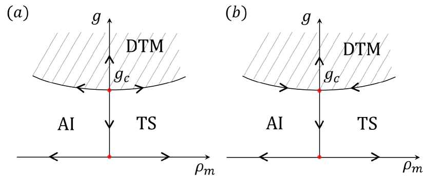
Figure 4: Possible RG-flow phase diagram for 2D Dirac fermion with random mass. (a) uniform mass is a relevant scaling variable around the fixed point at $g=g_{c}$; (b) uniform mass is an irrelevant scaling variable around the fixed point at $g=g_{c}$.

To clarify the scaling property of the uniform mass, we use the same perturbative renormalization theory as in the previous section and calculate the scaling dimension of the uniform mass operator up to the two-loop order (second order in $g$). To this end, we treat the uniform mass operator as an external perturbation and expand the vertex functions in terms of the uniform mass $m$ [35, 42, 36, 34]. Since the uniform mass has a dimension of $1$ at the clean-limit fixed point, ${\rm dim}[m]=1$, the $m$-linear term of the two-points vertex function has the UV logarithmic divergence in $d=2$. Namely, following the same line of the argument in Sec. IIIA, we expand the vertex functions at finite $m$ in terms of ${\bm{k}}$, $\omega$, and $m$ in $d=2$,

$$\Gamma^{(2)}_{\alpha}({\bm{k}},\omega,m)= \Gamma^{(2)}_{\alpha}({\bm{k}},\omega,m=0)$$

$$\ \ +(\cdots)\cdot\ln\Lambda\sigma_{3}\cdot m+{\cal O}(m^{2}).$$ (58)

Here a $m$-linear term in the four-points vertex function as well as the higher-order terms in $m$ in all the vertex functions have no UV divergence in the two dimensions. Thus, the bare theory in the presence of finite uniform mass have one additional logarithmic divergent term compared to the bare massless theory. The new UV divergent term can be absorbed into a renormalization of the mass $m$. We do this mass renormalization by using the same $\epsilon$-expansion as in the previous section, where $\ln\Lambda$ in the two dimensions is replaced by $1/\epsilon$ in the $d=2-\epsilon$ dimensions.

The replicated action with the uniform mass is given by an addition of the uniform mass term into $S_{\rm eff}$ and $Z_{\rm eff}$ in Eqs. (12), (11), and (17),

$$S_{\rm eff} =\cdots+\int_{{\bm{k}},\omega}\psi^{\dagger}_{\alpha}({\bm{k}},\omega)m\hat{\gamma}\psi_{\alpha}({\bm{k}},\omega).$$

Using the same minimal subtraction method as in the previous section, we rewrite the bare field in the mass term by the renormalized field,

$$S_{\rm eff} =\cdots+\int_{{\bm{k}},\omega}\phi^{\dagger}_{\alpha}({\bm{k}},\omega)\!\ (1+\delta_{M})M\!\ \hat{\gamma}\!\ \phi_{\alpha}({\bm{k}},\omega),$$ (59)

where the omitted parts in $S_{\rm eff}$ are already given in Eqs. (23) and (24). Namely, we put the added mass term as

$$m\psi^{\dagger}_{\alpha}\hat{\gamma}\psi_{\alpha}=Z_{2}Z^{-1}_{\cal O}M\phi^{\dagger}_{\alpha}\hat{\gamma}\phi_{\alpha}.$$ (60)

Here a renormalized mass $M$ and its counterterm $\delta_{M}$ are related to the bare mass $m$ as;

$$m\equiv Z^{-1}_{\cal O}M,\quad Z_{2}Z^{-1}_{\cal O}\equiv 1+\delta_{M},$$ (61)

with $Z_{2}$ the field renormalization defined in Eq. (25). The renormalized vertex functions are given as functions of ${\bm{k}}$, $\Omega$ and the renormalized mass $M$. We determine the previous counterterms ($\delta\Omega$, $\delta\kappa$, $\delta_{2}$) including $\delta_{M}$ in such a way that the following RG conditions are satisfied by the renormalized vertex functions;

$$\overline{\Gamma}^{(2)}_{\alpha}({\bm{k}},\Omega,M)\Big{|}_{M=0}=-i\Omega+{\bm{\gamma}}\cdot{\bm{k}}+{\cal O}(1),$$ (62)

$$\partial_{M}\overline{\Gamma}^{(2)}_{\alpha}({\bm{k}},\Omega,M)\Big{|}_{{\bm{k}}=0,M=0}=\hat{\gamma}+{\cal O}(1),$$ (63)

$$\overline{\Gamma}^{(4)}_{\alpha\beta}({\bm{k}}_{1},{\bm{k}}_{2},{\bm{k}}_{3}:\Omega_{1},\Omega_{2})\Big{|}_{{\bm{k}}_{i}=0,\Omega_{i}=\Omega,M=0}$$

$$\ \ =\Omega^{\epsilon}\kappa\hat{\gamma}\otimes\hat{\gamma}+{\cal O}(1).$$ (64)

Namely, such vertex functions are free from the UV divergence as functions of renormalized single-particle energy, renormalized uniform mass and renormalized disorder strength, e.g.

$$\overline{\Gamma}^{(2)}({\bm{k}},\Omega,M)=-i\Omega+{\bm{\gamma}}\cdot{\bm{k}}+M\hat{\gamma}+{\cal O}(1).$$ (65)

The first and the third conditions, Eq. (62) and (64), are already satisfied by $\delta_{2}$, $\delta\kappa$ and $\delta\Omega$ determined in the previous section. Thus, we have only to determine $\delta_{M}$ together with these counterterms such that the second condition Eq. (63) is satisfied.

$\partial_{M}\overline{\Gamma}^{(2)}_{\alpha}({\bm{k}},\Omega,M)$ evaluated at $M=0$ is nothing but an amputated one-particle irreducible (1PI) part of a composite Green function at the massless point (Fig. 5) [35, 42, 36, 34]. To see this, let us take the derivative of Eq. (28) with respect to the renormalized mass,

$$\partial_{M}\overline{\Gamma}^{(2)}_{\alpha}({\bm{k}},\Omega,M)\Big{|}_{{\bm{k}}=0,M=0}$$

$$\ \ =-\overline{G}^{-1}_{\alpha}\cdot\partial_{M}\overline{G}^{(2)}_{\alpha}({\bm{k}},\Omega,M)\Big{|}_{{\bm{k}}=0,M=0}\cdot\overline{G}^{-1}_{\alpha}.$$ (66)

From Eqs. (29) and (59), the derivative of the two-points Green function in the right hand side is given by the following composite Green function,

$$(2\pi)^{d+1}\delta^{d+1}(k-k^{\prime})\!\ \partial_{M}\overline{G}^{(2)}_{\alpha}({\bm{k}},\Omega,M)\Big{|}_{M=0}$$

$$\ \ =-(1+\delta_{M})\int_{k^{\prime\prime}}\langle\phi_{\alpha}(k)\phi^{\dagger}_{\epsilon}(k^{\prime\prime})\hat{\gamma}\phi_{\epsilon}(k^{\prime\prime})\phi^{\dagger}_{\alpha}(k^{\prime})\rangle_{{\rm eff},c},$$

$$\ \ \equiv-(1+\delta_{M})(2\pi)^{d+1}\delta^{d+1}(k-k^{\prime})\!\$$

$$\hskip 56.9055pt\times\overline{G}_{\alpha}({\bm{k}},\Omega)\overline{\Gamma}^{(2,1)}_{\alpha}({\bm{k}},\Omega)\overline{G}_{\alpha}({\bm{k}},\Omega),$$ (67)

with $\langle\cdots\rangle_{{\rm eff},c}\equiv\langle\phi_{\alpha}\phi^{\dagger}_{\epsilon}\hat{\gamma}\phi_{\epsilon}\phi^{\dagger}_{\alpha}\rangle_{\rm eff}-\langle\phi_{\alpha}\phi^{\dagger}_{\alpha}\rangle_{\rm eff}\langle\phi^{\dagger}_{\epsilon}\hat{\gamma}\phi_{\epsilon}\rangle_{\rm eff}$, $k\equiv({\bm{k}},\omega)$, $k^{\prime}\equiv({\bm{k}}^{\prime},\omega^{\prime})$ and $k^{\prime\prime}\equiv({\bm{k}}^{\prime\prime},\omega^{\prime\prime})$. Here $\langle\cdots\rangle_{\rm eff}$ in the right hand side is taken over $S_{\rm eff}$ with the zero uniform mass, $M=0$. The two inverse Green functions in Eq. (66) amputate one-particle reducible parts of the composite Green function;

$$\partial_{M}\Gamma^{(2)}_{\alpha}({\bm{k}},\Omega,M)\Big{|}_{M=0}=(1+\delta_{M})\overline{\Gamma}^{(2,1)}_{\alpha}({\bm{k}},\Omega).$$ (68)

In the following, the 1PI part of the amputated composite Green function $\overline{\Gamma}^{(2,1)}_{\alpha}({\bm{k}},\Omega)$ will be calculated at ${\bm{k}}=0$ perturbatively in $g$ in $d=2-\epsilon$ with the renormalized massless theory $S_{\rm eff}$ of Eqs. (23) and (24). The 1PI part thus obtained contains $1/\epsilon$ divergent terms. $\delta_{M}$ in the right hand side of Eq. (68) shall be chosen in such a way that all the $1/\epsilon$ divergent terms in $\overline{\Gamma}^{(2,1)}_{\alpha}({\bm{k}}=0,\Omega)$ are cancelled by $\delta_{M}$, satisfying Eq. (63).

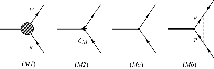
Figure 5: (M1) Feynman diagrams of the 1-particle irreducible (1PI) part of $(1+\delta_{M})\overline{\Gamma}^{(2,1)}_{\alpha}({\bm{k}},\Omega)$. ($M2$) The zero-th order in $g$ for $\delta_{M}\overline{\Gamma}^{(2,1)}_{\alpha}({\bm{k}},\Omega)$. ($Ma$) The zero-th order in $g$ for $\overline{\Gamma}^{(2,1)}_{\alpha}({\bm{k}},\Omega)$. ($Mb$) The first order in $g$ for $\overline{\Gamma}^{(2,1)}_{\alpha}({\bm{k}},\Omega)$.

The zero-th and the first order contributions to the right hand side of Eq. (68) are shown in Fig. 5. $[Ma]$ and $[M2]$ comprise the zero-th order contribution to the 1PI part of $(1+\delta_{M})\overline{\Gamma}^{(2,1)}_{\alpha}({\bm{k}},\Omega)$;

$$[Ma]=\hat{\gamma},\quad[M2]=\delta_{M}^{(1)}\hat{\gamma}.$$

As in Eq. (44), $\delta^{(m)}_{M}$ stands for the $m$-loop contribution to the counterterm $\delta_{M}$; $\delta_{M}\equiv\sum_{m}\delta^{(m)}_{M}$. A one-loop diagram $[Mb]$ is the first order contribution to $\overline{\Gamma}^{(2,1)}_{\alpha}({\bm{k}},\Omega)$;

$$[Mb]=\kappa\Omega^{\epsilon}\int_{\bm{p}}\frac{1}{-i\Omega-\bm{\gamma}\cdot\bm{p}}\cdot\frac{1}{-i\Omega+\bm{\gamma}\cdot\bm{p}}\hat{\gamma}$$

$$= \kappa\Omega^{\epsilon}\cdot\Big{(}-\frac{C_{2-\epsilon}}{\epsilon}{\Omega}^{-\epsilon}\Big{)}\hat{\gamma}+\mathcal{O}(1)=-\frac{g}{2\epsilon}\hat{\gamma}+\mathcal{O}(1).$$ (69)

The one-loop counterterm $\delta_{M}^{(1)}$ should cancel this $1/\epsilon$ divergence,

$$\delta^{(1)}_{M}=\frac{g}{2\epsilon},$$ (70)

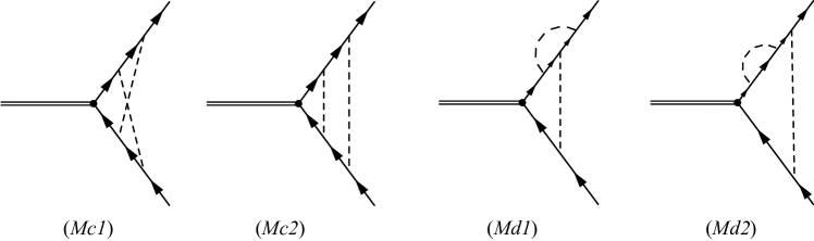
Figure 6: Two-loop Feynman diagrams of the 1PI part of $(1+\delta_{M})\overline{\Gamma}^{(2,1)}_{\alpha}({\bm{k}},\Omega)$.

The two-loop contributions to the 1PI part of $(1+\delta_{M})\overline{\Gamma}^{(2,1)}_{\alpha}({\bm{k}},\Omega)$ are shown in Fig. 6 and Fig. 7. All these diagrams are evaluated at ${\bm{k}}=0$, and take a form of $\hat{\gamma}$ (see below). We will evaluate their coefficients of $\hat{\gamma}$ in the following. The coefficient of $\hat{\gamma}$ in the diagram $[Mc1]$ is calculated as follows;

$$[Mc1]=\kappa^{2}\Omega^{2\epsilon}\int_{\bm{p},\bm{q}}\frac{1}{-i\Omega+\bm{\gamma}\cdot\bm{q}}\cdot\frac{1}{-i\Omega-\bm{\gamma}\cdot\bm{p}}$$

$$\times\frac{1}{-i\Omega+\bm{\gamma}\cdot\bm{p}}\cdot\frac{1}{-i\Omega-(\bm{\gamma}\cdot\bm{p}-\bm{\gamma}\cdot\bm{q})}$$

$$= -\kappa^{2}\Omega^{2\epsilon}\int_{\bm{p},\bm{q}}\frac{\bm{p}\bm{q}+q^{2}-\Omega^{2}}{(\Omega^{2}+\bm{q}^{2})(\Omega^{2}+\bm{p}^{2})\big{(}\Omega^{2}+(\bm{p}+\bm{q})^{2}\big{)}}$$

$$= \kappa^{2}\Omega^{2\epsilon}\Big{[}\frac{1}{2}\Big{(}\frac{C_{d}}{\epsilon}\Omega^{-\epsilon}\Big{)}^{2}-\Big{(}\frac{C_{d}}{\epsilon}\Omega^{-\epsilon}\Big{)}^{2}\Big{]}+\mathcal{O}(1)$$

$$= -\frac{1}{2}\frac{g^{2}}{4\epsilon^{2}}+\mathcal{O}(1).$$ (71)

The coefficients of $\hat{\gamma}$ in the diagrams $[Mc2]$, $[Md1]$ and $[Md2]$ are calculated as follows;

$$[Mc2]= \kappa^{2}\Omega^{2\epsilon}\int_{\bm{p},\bm{q}}\frac{1}{-i\Omega+\bm{\gamma}\cdot\bm{q}}\cdot\frac{1}{-i\Omega-\bm{\gamma}\cdot\bm{p}}$$

$$\times\frac{1}{-i\Omega+\bm{\gamma}\cdot\bm{p}}\cdot\frac{1}{-i\Omega-\bm{\gamma}\cdot\bm{q}}$$

$$= \kappa^{2}\Omega^{2\epsilon}\Big{(}\frac{C_{2-\epsilon}}{\epsilon}{\Omega}^{-\epsilon}+\mathcal{O}(\epsilon)\Big{)}^{2}=\frac{g^{2}}{4\epsilon^{2}}+\mathcal{O}(1),$$ (72)

$$[Md1]= \kappa^{2}\Omega^{2\epsilon}\int_{\bm{p},\bm{q}}\overline{G}_{0}(\bm{q})\overline{G}_{0}(-\bm{q}-\bm{p})\overline{G}_{0}(\bm{p})\overline{G}_{0}(-\bm{p})$$

$$= \kappa^{2}\Omega^{2\epsilon}\frac{1}{2}\Big{(}\frac{C_{d}}{\epsilon}\Omega^{-\epsilon}\Big{)}^{2}+\mathcal{O}(1)=\frac{g^{2}}{8\epsilon^{2}}+\mathcal{O}(1),$$ (73)

$$[Md2]= \kappa^{2}\Omega^{2\epsilon}\int_{\bm{p},\bm{q}}\overline{G}_{0}(\bm{p})\overline{G}_{0}(-\bm{q})\overline{G}_{0}(\bm{p})\overline{G}_{0}(-\bm{p})$$

$$= \frac{g^{2}}{8\epsilon}+\mathcal{O}(1).$$ (74)

The two-loop contributions to $(1+\delta_{M})\overline{\Gamma}^{(2,1)}_{\alpha}({\bm{k}},\Omega)$ that contain one-loop counterterms are shown in Fig. 7. The diagram $[Me]$ contains $\delta\kappa$’s one-loop counterterm,

$$[Me]=\Omega^{\epsilon}\delta^{(1)}\kappa\int_{\bm{p}}\frac{1}{-i\Omega-\bm{\gamma}\cdot\bm{p}}\cdot\frac{1}{-i\Omega+\bm{\gamma}\cdot\bm{p}}$$

$$= \frac{\Omega^{\epsilon}}{2C_{d}}\frac{g^{2}}{\epsilon}\Big{(}-\frac{C_{2-\epsilon}}{\epsilon}{\Omega}^{-\epsilon}+\mathcal{O}(\epsilon)\Big{)}=-\frac{g^{2}}{2\epsilon^{2}}+\mathcal{O}(1).$$ (75)

The diagrams $[Mf1]$ and $[Mf2]$ are the $\kappa$’s first-order terms that contain the $\delta\Omega$’s one-loop counterterm. A sum of these two is calculated as follows,

$$[Mf1]+[Mf2]=2\kappa\Omega^{\epsilon}\!\ i\delta^{(1)}\Omega\!\ \int_{\bm{p}}\overline{G}_{0}(\bm{p})\overline{G}_{0}(\bm{p})\overline{G}_{0}(-\bm{p})$$

$$= 2\kappa\Omega^{\epsilon}\big{(}-i\Omega\big{)}^{2}\frac{g}{2\epsilon}\Big{(}\frac{1}{2}C_{2-\epsilon}\Omega^{-2-\epsilon}+\mathcal{O}(\epsilon)\Big{)}$$

$$= -\frac{g^{2}}{4\epsilon}+\mathcal{O}(1).$$ (76)

The diagram $[Mg]$ is the $\kappa$’s first-order contribution to $\delta_{M}\overline{\Gamma}^{(2,1)}_{\alpha}({\bm{k}},\Omega)$. Up to the second order in $g$, we use Eq. (70) as $\delta_{M}$,

$$[Mg]= \delta^{(1)}_{M}\cdot\kappa\Omega^{\epsilon}\int_{\bm{p}}\frac{1}{-i\Omega-\bm{\gamma}\cdot\bm{p}}\cdot\frac{1}{-i\Omega+\bm{\gamma}\cdot\bm{p}}$$

$$= \frac{g}{2\epsilon}\cdot\kappa\Omega^{\epsilon}\int_{\bm{p}}\frac{-1}{\Omega^{2}+p^{2}}=-\frac{g^{2}}{4\epsilon^{2}}+\mathcal{O}(1).$$ (77)

By taking into account appropriate symmetry factors in each diagram, we let the two-loop counterterm $\delta^{(2)}_{M}$ cancels the $1/\epsilon$ divergent terms in Eq. (68):

$$\delta^{(2)}_{M} =-\big{(}[Mc1]+[Mc2]+2[Md1]+2[Md2]$$

$$\quad+[Me]+[Mf1]+[Mf2]+[Mg]\big{)}=\frac{3g^{2}}{8\epsilon^{2}}.$$ (78)

Combining Eqs. (70) and (78), we finally obtain the mass renormalization constant $Z_{\cal O}$ up to the two-loop level as follows,

$$Z_{\mathcal{O}}^{-1}= Z^{-1}_{2}(1+\delta^{(1)}_{M}+\delta^{(2)}_{M})=1+\frac{g}{2\epsilon}-\frac{g^{2}}{16\epsilon}+\frac{3g^{2}}{8\epsilon^{2}}.$$ (79)

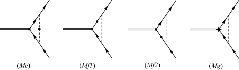
Figure 7: Two-loop contributions to the 1PI part that contains one-loop counterterms, such as $\delta^{(1)}\kappa$, $\delta^{(1)}\Omega$, and $\delta^{(1)}_{M}$. Note that as shown in the previous section, $\delta_{2}$ starts from the second order in $g$, so that it does not contribute to these diagrams.

The two-points vertex function has been renormalized up to the linear order in the uniform mass, Eq. (65). The UV divergent terms of the bare two-points vertex function are included in the renormalization constants at the finite RG scale $\Omega$. The renormalized vertex functions in the small $\Omega$ limit determine ground-state property of $S_{\rm eff}$ with a finite uniform mass. When the RG scale $\Omega$ goes to zero with fixed bare uniform mass $m$ and a fixed bare disorder strength $\Delta_{3}$, the renormalized mass $M$ changes its value according to Eq. (61). The renormalized $M$ thus changed determines the ground-state property of $S_{\rm eff}$ with a finite (but small) uniform mass (see below). To determine how $M$ changes in the small $\Omega$ limit, let us take an $\Omega$ derivative of Eq. (61) with a fixed $m$ and $\Delta_{3}$,

$$0\equiv \frac{\partial\ln m}{\partial\ln\Omega}\Big{|}_{\Delta_{3},m}=\frac{\partial\ln M}{\partial\ln\Omega}\Big{|}_{\Delta_{3},m}-\frac{\partial\ln Z_{\mathcal{O}}}{\partial\ln\Omega}\Big{|}_{\Delta_{3},m}.$$ (80)

This gives an anomalous dimension of the uniform mass, $\gamma_{\cal O}$,

$$\frac{\partial\ln M}{\partial\ln\Omega}\Big{|}_{\Delta_{3},m} =\frac{\partial g}{\ln\Omega}\Big{|}_{\Delta_{3},m}\frac{d\ln Z_{\mathcal{O}}}{dg}$$

$$=\beta_{g}\frac{d\ln Z_{\mathcal{O}}}{dg}\equiv\gamma_{\cal O}.$$ (81)

From Eqs. (79) and (56), we obtain the two-loop evaluation of the anomalous dimension of the uniform mass:

$$\gamma_{\mathcal{O}}\equiv\beta_{g}\frac{\partial\ln Z_{\mathcal{O}}}{\partial g}=\frac{g}{2}-\frac{g^{2}}{8}.$$ (82)

In the clean limit ($g=0$), $\gamma_{\mathcal{O}}=0$, while $\gamma_{\mathcal{O}}$ can be non-zero around a fixed point with finite $g$. With an introduction of a renormalized dimensionless uniform mass $\rho_{m}$ as $M\equiv\Omega\rho_{m}$, a scaling property of $\rho_{m}$ around the massless theory is obtained as follows,

$$\frac{\partial\rho_{m}}{\partial l}=(1-\gamma_{\mathcal{O}})\rho_{m}\equiv d_{m}\rho_{m},$$ (83)

with $l\equiv-\ln\Omega$. The two-loop scaling dimension of the renormalized dimensionless uniform mass is finally obtained around a massless fixed point ($\rho_{m}=0$) as

$$d_{m}=1-\frac{g}{2}+\frac{g^{2}}{8}.$$ (84)

V RG phase diagram of two-dimensional Dirac fermion with random mass

In the previous section, the two-loop RG equations for the disorder strength and uniform mass as well as the dynamical exponent are evaluated perturbatively in the disorder strength around the clean-limit fixed point in $d=2-\epsilon$, Eqs. (56), (84), and (57). In this section, we set $\epsilon=0$, and study a structure of a RG phase diagram for the random-mass Dirac fermions in the two dimensions,

$$\begin{cases}\displaystyle\frac{\partial g}{\partial l}=-\beta_{g}=\,-g^{2}+\frac{g^{3}}{2},\phantom{\frac{}{\phantom{\displaystyle\frac{1}{}}}}\\ \displaystyle\frac{\partial\rho_{m}}{\partial l}=\,d_{m}\rho_{m}=\Big{(}1-\frac{g}{2}+\frac{g^{2}}{8}\Big{)}\rho_{m},\end{cases}$$ (85)

$$\quad z=\,1+\frac{g}{2}+\frac{g^{2}}{8}.$$ (86)

Here $g$, $\rho_{m}$ and $z$ stand for the dimensionless random-mass-type disorder strength, the dimensionless uniform mass, and the dynamical exponent respectively.

In the low-energy limit ($l\rightarrow+\infty$), the two coupling constants flow in the $g$-$\rho_{m}$ parameter space, forming a phase diagram as shown in Fig. 1. The RG phase diagram comprises of three phases, a diffusive thermal metal (DTM) with larger $g$, a topological superconductor (TS) with $g=0$ and $\rho_{m}>0$, and a conventional Anderson insulator (AI) with $g=0$ and $\rho_{m}<0$. The three phases meet at an IR unstable fixed point at $(g,\rho_{m})=(g_{c},0)$, that can be regarded as the multicritical (tricritical) point in the preceding numerical phase diagram of the CF model  [11, 14].

In the massless case ($\rho_{m}=0$), the fixed point at $g=g_{c}$ corresponds to a semimetal-metal (SM-M) quantum phase transition point. For $g<g_{c}$ and $\rho_{m}=0$, the finite disorder strength is renormalized to zero in the low-energy limit, where the ground state is characterized by the clean-limit massless Dirac-fermion fixed point at $(g,\rho_{m})=(0,0)$ (semimetal phase). For $g>g_{c}$, the disorder strength grows up into a larger value. The ground state for $g>g_{c}$ is in a diffusive metal phase, which is presumably described by another stable fixed point at larger $g$. The criticality of the SM-M quantum phase transition point at $\rho_{m}=0$ is controlled by the fixed point at $g=g_{c}$. Since the weak disorder strength ($g<g_{c}$) is renormalized to zero, universality class of a phase transition between AI and TS phases is determined by the clean-limit massless Dirac-fermion fixed point. According to the mapping between the random-mass Dirac fermion model and the random-bond Ising model (RBIM), the massless Dirac-fermion fixed point corresponds to the clean-limit Ising fixed point in the RBIM  [11].

The renormalized uniform mass is a relevant operator not only around the clean-limit massless Dirac-fermion fixed point but also around the fixed point at $g=g_{c}$. Accordingly, universality classes of the phase transition(s) between AI and DTM as well as that between TS and DTM must be determined by other saddle-point fixed point(s) at finite $\rho_{m}$. Exploring these fixed points at finite $\rho_{m}$ goes beyond the scope of this paper and we leave it for future study. Two-loop evaluations of the critical disorder strength, the scaling dimensions of the disorder strength and the uniform mass, and the dynamical exponent around the unstable fixed point are $g_{c}=2$, ${\rm dim}[g-g_{c}]=2$, ${\rm dim}[\rho_{m}]=1/2$, and $z(g_{c})=5/2$, respectively.

A correlation-length critical exponent for the SM-M quantum phase transition at the massless case is obtained from the following relation

$$\frac{\partial\ln(g-g_{c})}{\partial l}=\nu^{-1}$$ (87)

with $\nu(g_{c})=1/2$ at the two-loop level. This critical exponent violates the Chayes inequality, that dictates $\nu d\geq 2$ with the spatial dimension $d$ [43]. To see whether the inequality holds or not at the higher order in $g$, we evaluate in the next section the correlation-length critical exponent up to the four-loop level, using a relation between the effective theory $S_{\rm eff}$ and SU(N) Gross-Neveu (GN) model.

VI higher-loop results deduced from mappings to other models

VI.1 Transformation between random-mass and random-chemical-potential in Dirac fermions in two dimensions

The 2-loop RG equation [Eq. (85)] is consistent with the previous studies of random Dirac fermion with chemical-potential-type disorder, under a transformation between random mass and random chemical potential [27, 38]. To explain this transformation, we start from the 2D replicated action for the random-mass Dirac fermion Eq. (9),

$$S_{0}= \int d\tau d^{2}\bm{x}\,\psi_{\alpha}^{\dagger}\Big{\{}\partial_{\tau}-iv(\partial_{1}\sigma_{1}+\partial_{2}\sigma_{2})+m\sigma_{3}\Big{\}}\psi_{\alpha},$$

$$S_{1}= -\frac{\Delta_{3}}{2}\!\int\!d\tau d\tau^{\prime}d^{2}\bm{x}\big{(}\psi_{\alpha}^{\dagger}\sigma_{3}\psi_{\alpha}\big{)}_{\bm{x},\tau}\big{(}\psi_{\beta}^{\dagger}\sigma_{3}\psi_{\beta}\big{)}_{\bm{x},\tau^{\prime}}.$$ (88)

In the path integral formulation, $\psi^{\dagger}$ and $\psi$ can be considered as independent integral variables. Thus, we can define a new set of integral variables $\{\bar{\psi},\psi\}$ as  [44],

$$\psi^{\dagger}\rightarrow\bar{\psi}=-i\psi^{\dagger}\sigma_{3},\quad\psi^{\dagger}=i\bar{\psi}\sigma_{3}$$ (89)

while keeping $\psi$ unchanged. The action of Eq. (88) with $\{\bar{\psi},\psi\}$ is given by,

$$S_{0}= \int d\tau d^{2}\bm{x}\,\bar{\psi}_{\alpha}\Big{\{}(i\sigma_{3})\partial_{\tau}+iv(\sigma_{2}\partial_{1}-\sigma_{1}\partial_{2})+im\Big{\}}\psi_{\alpha},$$

$$S_{1}= +\frac{\Delta_{3}}{2}\int d\tau d\tau^{\prime}d^{2}\bm{x}\,\big{(}\bar{\psi}_{\alpha}\psi_{\alpha}\big{)}_{\bm{x},\tau}\big{(}\bar{\psi}_{\beta}\psi_{\beta}\big{)}_{\bm{x},\tau^{\prime}}.$$ (90)

Under an SU(2) rotation by the 90 degree,

$$\psi\rightarrow e^{i\frac{\pi}{4}\sigma_{3}}\psi,\quad\bar{\psi}\rightarrow\bar{\psi}e^{-i\frac{\pi}{4}\sigma_{3}},$$

the action with $\{\bar{\psi},\psi\}$ can be put into the following form,

$$S_{0}= \int d\tau d^{2}\bm{x}\,\bar{\psi}_{\alpha}\Big{\{}(i\sigma_{3})\partial_{\tau}-iv(\sigma_{1}\partial_{1}+\sigma_{2}\partial_{2})+im\Big{\}}\psi_{\alpha},$$

$$S_{1}= +\frac{\Delta_{3}}{2}\int d\tau d\tau^{\prime}d^{2}\bm{x}\,\big{(}\bar{\psi}_{\alpha}\psi_{\alpha}\big{)}_{\bm{x},\tau}\big{(}\bar{\psi}_{\beta}\psi_{\beta}\big{)}_{\bm{x},\tau^{\prime}}.$$ (91)

This action is related to a replicated effective theory for the random Dirac fermion with the chemical-potential-type disorder potential, [27, 38, 44]

$$S_{0}^{\prime}= \int d\tau d^{2}\bm{x}\,\bar{\psi}_{\alpha}\Big{\{}\partial_{\tau}-iv(\sigma_{1}\partial_{1}+\sigma_{2}\partial_{2})+\tilde{m}\sigma_{3}\Big{\}}\psi_{\alpha},$$

$$S_{1}^{\prime}= -\frac{\Delta_{0}}{2}\int d\tau d\tau^{\prime}d^{2}\bm{x}\,\big{(}\bar{\psi}_{\alpha}\psi_{\alpha}\big{)}_{\bm{x},\tau}\big{(}\bar{\psi}_{\beta}\psi_{\beta}\big{)}_{\bm{x},\tau^{\prime}}.$$ (92)

Here $\tilde{m}$ and $\Delta_{0}$ stand for bare uniform mass and chemical-potential-type disorder strength. The two theories are mapped to each other, where $i\partial_{\tau}$, $im$ and $\Delta_{3}$ in Eq. (91) correspond to $\tilde{m}$ and $\partial_{\tau}$ and $-\Delta_{0}$ in Eq. (92), respectively. In the latter theory, the preceding work employed the renormalized single-particle energy as the RG scale and derive two-loop RG equation for the disorder strength $\Delta_{0}$ [38, 39, 45, 40]. One could also use the renormalized uniform mass as the RG scale, to derive the same two-loop RG equation. Thanks to the correspondence between Eq. (91) and Eq. (92), such two-loop RG equation must be identical to Eq. (56) under the sign change of the disorder strength, $\Delta_{0}\leftrightarrow-\Delta_{3}$. In fact, this is the case up to the two-loop level [38, 39, 45, 40].

VI.2 Relation to (1+1) dimensional SU(N) Gross-Neveu model

The replicated 2D Dirac fermion theory with mass-type disorder Eq. (88) as well as that with chemical-potential-type disorder Eq. (92) are related to ($d$+1)D SU(N) Gross-Neveu (GN) model  [46, 45, 47],

$$S_{\text{GN}}=\int d\tau d^{d}{\bm{x}}\bigg{\{}\bar{\psi}_{a}i\big{(}\partial_{\mu}\gamma^{\mu}-m\big{)}\psi_{a}+\frac{\bar{g}}{2}\big{(}\bar{\psi}_{a}\psi_{a}\big{)}^{2}\bigg{\}},$$ (93)

with $a=1,2,\cdots,N$. The Dirac matrices $\{\gamma^{\mu}=\gamma_{\mu}\}$ ($\mu=0,1,\cdots,d$) satisfy the relation $\{\gamma_{\mu},\gamma_{\nu}\}=2\delta_{\mu\nu}$ in $(d+1)$ Euclidean space time. The conjugate of the Dirac filed is defined as $\bar{\psi}=i\psi^{\dagger}\gamma^{0}$. In the $(1+1)$-dimension, a representation of $\gamma^{\mu}$ matrices reduces to the two by two Pauli matrices,

$$\gamma^{0}=\sigma_{1},\quad\gamma^{1}=\sigma_{2},\quad\gamma^{0}\gamma^{1}=i\sigma_{3}.$$ (94)

Note that the quenched disorder in Eq. (91) does not change the frequency of fermion lines, so that the fermion frequencies can be regarded as an external parameter. Accordingly, Eq. (91) in the two-spatial dimension in the zero replica limit ($R\rightarrow 0$) and Eq. (93) in the $(1+1)$-dimension in the limit of $N\rightarrow 0$ share the same renormalization group theory, where $\partial_{1}$, $\partial_{2}$, $\Delta_{3}$, $m$ and $v$ in Eq. (91) are replaced by $\partial_{0}$, $\partial_{1}$, $\bar{g}$, $m$ and $1$ in Eq. (93), respectively [47].

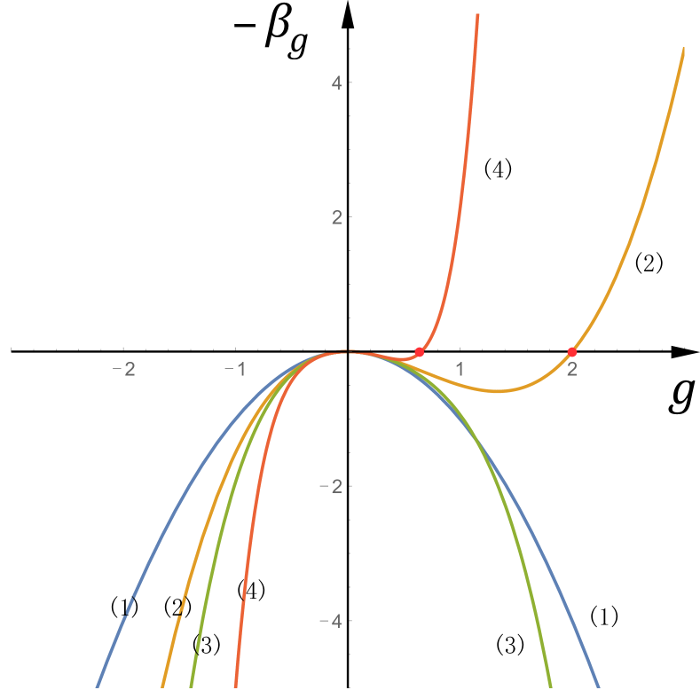
Figure 8: The $m$-loop $\beta$ function for coupling constant $g$ with $m=1,2,3,4$. The two-loop and four-loop $\beta$ function show a zero point at positive values of $g$.

The $\beta$ function for the GN coupling constant $\beta_{g}$ and the anomalous dimension $\gamma_{m}$ of the uniform mass $m$ have been calculated up to the four-loop order  [28, 29]. In the limit of $N\rightarrow 0$, they are given by

$$\beta_{\bar{g}}\big{|}_{N=0}=(d-2)\bar{g}+\frac{\bar{g}^{2}}{\pi}-\frac{\bar{g}^{3}}{2\pi^{2}}+\frac{7\bar{g}^{4}}{16\pi^{3}}-\frac{17\zeta_{3}+4}{8\pi^{4}}\bar{g}^{5},$$

$$\gamma_{m}\big{|}_{N=0}=\frac{\bar{g}}{2\pi}-\frac{\bar{g}^{2}}{8\pi^{2}}+\frac{3\bar{g}^{3}}{32\pi^{3}}-\frac{[52\zeta_{3}+19]}{128\pi^{4}}\bar{g}^{4},$$ (95)

where $\overline{g}$ corresponds to $\Delta_{3}$ in Eq. (91). $\zeta_{3}$ is a value of Riemann zeta function $\zeta_{3}=\zeta(3)$ (Apéry’s constant). To compare these equations with Eq. (85), we normalize $\overline{g}\equiv\Delta_{3}$ by $\pi$ in the two dimensions from Eqs. (33) and (27)

$$g=2C_{2}\Delta_{3}=\frac{\overline{g}}{\pi}.$$ (96)

With this normalization, Eq. (95) is translated into the following $\beta$ functions for $g$ and the uniform mass $\rho_{m}$ for the 2D random-mass Dirac fermions,

$$\begin{cases}\displaystyle\frac{\partial g}{\partial l}=\,-g^{2}+\frac{g^{3}}{2}-\frac{7}{16}g^{4}+\frac{17\zeta_{3}+4}{8}g^{5},\phantom{\frac{}{\phantom{\displaystyle\frac{1}{}}}}\\ \displaystyle\frac{\partial\rho_{m}}{\partial l}=\,\Big{(}1-\frac{g}{2}+\frac{g^{2}}{8}-\frac{3g^{3}}{32}+\frac{52\zeta_{3}+19}{128}g^{4}\Big{)}\rho_{m}.\end{cases}$$ (97)

At the two-loop level, Eq. (85) has the IR unstable fixed point at $g_{c}=2$, which corresponds to the multicritical (tricritical) point. At the four-loop level, this critical disorder strength moves to a smaller value, $g_{c}\approx 0.655$. Fig. 8 shows the $\beta$ function of $g$ for the $1,2,3,4$-loop order.

The four-loop evaluation of the scaling dimension of $g-g_{c}$ and the uniform mass around the fixed point are ${\rm dim}[g-g_{c}]\approx 1.66$ and ${\rm dim}[\rho_{m}]\approx 0.817$ respectively. The critical exponent associated with the SM-M quantum phase transition is evaluated as $\nu\approx 0.60$, which also violates the Chayes inequality.

VII Summary and Discussion

In summary, we have performed renormalization group analyses for the 2D Dirac fermion with the random-mass type disorder. We obtained the two-loop $\beta$ function for the disorder strength and observed an infrared unstable fixed point at a finite disorder strength. The fixed point corresponds to the quantum tricritical point that intervenes diffusive metal phase, and two topologically distinct gapped phases in 2-dimensional class D models. Two phase transition lines between the diffusive metal and the two gapped phases and a transition line between the two topologically-distinct gapped phases meet at the tricritical point. The dynamical exponent and scaling dimension of the uniform mass are also evaluated at the tricritical point up to the two-loop level.

The two-loop evaluations of the scaling dimensions of the uniform mass and disorder strength shows that (i) the transition line between the two gapped phases is controlled by the clean-limit massless-Dirac-fermion fixed point with the Ising criticality, (ii) the transition lines between the diffusive metal phase and gapped phases are controlled not by the tricritical point but by another saddle-point fixed point with finite uniform Dirac mass. Using a mapping between the effective theory for the 2D random-mass Dirac fermion and (1+1)D SU(N) Gross-Neveu model in the limit of $N\rightarrow 0$, we also obtained the four-loop evaluations of the scaling dimensions of the uniform mass and disorder strength around the tricritical point. The four-loop result gives the same conclusion as the two-loop result about the criticality of the three transition lines. We found that the critical exponent $\nu$ for the semimetal-metal(SM-M) quantum phase transition breaks the Chayes inequality ($\nu d>1$) both at the two-loop level and at the four-loop level, indicating an unusual aspect of the disorder-driven SM-M quantum phase transition in 2D class D models.

Appendix A disordered Dirac Hamiltonian and replicated Dirac-fermions action

In the main text, the renormalization of the Green functions of replicated Driac fermions is intensively studied. The study leads to the renormalization group equation for the 2D Dirac fermions with random mass. In this appendix, we review an equivalence between averaged Green functions for disordered Dirac Hamiltonian and Green functions for the replicated Dirac fermions action $S_{\rm eff}$. A partition function for the disordered Dirac Hamiltonian is considered,

$$Z\big{[}\{V_{3}({\bm{r}})\}\big{]}\equiv\int{D}\psi^{\dagger}{D}\psi\,e^{-S\big{[}\{V_{3}({\bm{r}})\}\big{]}},\ \ S\big{[}\{V_{3}({\bm{r}})\}\big{]}\equiv\int_{-\beta/2}^{\beta/2}d\tau\,\big{(}\int d^{2}\bm{x}\psi^{\dagger}\partial_{\tau}\psi+\hat{H}\big{[}\{V_{3}({\bm{r}})\}\big{]}\big{)},$$ (98)

where an integral over an imaginary time $\tau$ ranges from $-\beta/2$ to $\beta/2$ with an inverse temperature $\beta\equiv 1/k_{B}T$. In the main text, we always take $\beta\rightarrow+\infty$ ($T=0$). A time-ordered $2n$-points Green function is given by a trace over the action in Eq. (98),

$$\langle\psi(1)\cdots\psi^{\dagger}(2n)\rangle=\frac{1}{Z}\int{D}\psi^{\dagger}{D}\psi\,\psi(1)\cdots\psi^{\dagger}(2n)e^{-S},$$ (99)

with space-time coordinates $i\equiv(\tau_{i},\bm{x}_{i})$ ($i=1,\cdots,2n$). The Green function is averaged over different disorder realization through the Gaussian distribution,

$$\langle(\cdots)\rangle_{\text{dis}}\equiv\frac{1}{\mathcal{N}}\int DV_{3}\,\big{(}\cdots\big{)}\!\ \exp\big{(}-\frac{1}{2\Delta_{3}}\int d^{2}\bm{x}V_{3}(\bm{x})^{2}\Big{)}.$$ (100)

where $\mathcal{N}$ is a normalization factor such that $\langle 1\rangle_{\text{dis}}=1$. The averaged Green function is given by,

$$\langle\langle\psi(1)\cdots\psi^{\dagger}(2n)\rangle\rangle_{\text{dis}}=\frac{1}{\mathcal{N}}\int DV_{3}\,\langle\psi(1)\cdots\psi^{\dagger}(2n)\rangle\,\exp\big{(}-\frac{1}{2\Delta_{3}}\int V_{3}^{2}\big{)}.$$ (101)

To treat the disorder-averaged $2n$-points Green functions systematically, we use a replica method throughout the paper [33, 34]. In the replica method, we introduce a replicated action that comprises of $R$-numbers of the identical free Dirac-fermion Hamiltonians of $\hat{H}_{0}$ and an elastic-scattering interaction between the replicated Dirac fermions, $S_{\rm eff}$ in Eq. (9). The averaged $2n$-points connected Green functions are given by the replica-limit of $2n$-points Green functions for the replicated Dirac-fermion action (9) [34]. The averaged two-points Green function is given by,

$$\langle\langle\psi(\bm{x},\tau)\psi^{\dagger}(\bm{x}^{\prime},\tau^{\prime})\rangle\rangle_{\text{dis}}=\lim_{R\rightarrow 0}\langle\psi_{\alpha}(\bm{x},\tau)\psi_{\alpha}^{\dagger}(\bm{x}^{\prime},\tau^{\prime})\rangle_{\text{eff}},$$ (102)

where the summation over the replica index is not assumed in the right hand side. $\langle\cdots\rangle_{\text{eff}}$ in the right hand side stands for a trace over the replicated action with the elastic interaction,

$$\langle\cdots\rangle_{\text{eff}}\equiv\frac{1}{Z_{\text{eff}}}\int{D}\psi_{\alpha}^{\dagger}{D}\psi_{\alpha}\,\big{(}\cdots\big{)}\,e^{-S_{\text{eff}}},\!\ \!\ Z_{\text{eff}}\equiv\int{D}\psi_{\alpha}^{\dagger}{D}\psi_{\alpha}\,e^{-S_{\text{eff}}}.$$ (103)

The averaged 4-points connected Green function is given by the four-points Green function of the replicated action in the replica limit,

$$\langle\langle\psi(1)\psi(2)\psi^{\dagger}(2^{\prime})\psi^{\dagger}(1^{\prime})\rangle_{c}\rangle_{\text{dis}} =\lim_{R\rightarrow 0}\frac{1}{R}\sum_{\alpha_{1},\alpha_{2},\beta_{2},\beta_{1}}\!\ \int{D}\psi_{\alpha}^{\dagger}{D}\psi_{\alpha}\,\psi_{\alpha_{1}}(1)\psi_{\alpha_{2}}(2)\psi_{\beta_{2}}^{\dagger}(2^{\prime})\psi_{\beta_{1}}^{\dagger}(1^{\prime})\,e^{-S_{\text{eff}}},$$

$$=\lim_{R\rightarrow 0}\frac{1}{R}\sum_{\alpha_{1},\alpha_{2},\beta_{2},\beta_{1}}\langle\psi_{\alpha_{1}}(1)\psi_{\alpha_{2}}(2)\psi_{\beta_{2}}^{\dagger}(2^{\prime})\psi_{\beta_{1}}^{\dagger}(1^{\prime})\rangle_{\rm eff}.$$ (104)

Similarly, the equivalence between the disorder-averaged $2n$-points connected Green function of the disordered single-particle Hamiltonian and $2n$-points Green function of the replicated action in the replica limit holds true for the higher order.

Appendix B Two-loop renormalization to the four–points vertex function

In this Appendix, the two-loop contribution to the four-points vertex counterterm is calculated in details. The two-loop contributions to the right hand side of Eq. (32) are given by Feynman diagrams in Figs. 9, 10, 11, 12, 13, and 14. Note that each of them could have divergent terms with tensor forms other than $\hat{\gamma}\otimes\hat{\gamma}$. We will show in this appendix that such divergent terms cancel exactly in the summation: the sum only gives divergent terms with the tensor form of $\hat{\gamma}\otimes\hat{\gamma}$. As in Eq. (32), the vertex function is evaluated with zero external momenta and with the two external frequencies set to $\Omega$. Accordingly, all the internal fermion lines carry the same frequency $\Omega$ and we thus abbreviate $\overline{G}_{0}({\bm{p}},\Omega)$ for internal fermion lines as $\overline{G}_{0}({\bm{p}})$ in the following.

All the diagrams in Fig. 9 give the divergent terms with $\hat{\gamma}\otimes\hat{\gamma}$.

$$[V2A]= \kappa^{3}\Omega^{3\epsilon}\int_{\bm{p},\bm{q}}\hat{\gamma}\overline{G}_{0}(\bm{p})\hat{\gamma}\overline{G}_{0}(\bm{q})\hat{\gamma}\overline{G}_{0}(\bm{q})\hat{\gamma}\overline{G}_{0}(\bm{p})\hat{\gamma}\otimes\hat{\gamma},$$ (105)

$$[V2B]= \kappa^{3}\Omega^{3\epsilon}\int_{\bm{p},\bm{q}}\hat{\gamma}\overline{G}_{0}(\bm{p})\hat{\gamma}\overline{G}_{0}(\bm{p}+\bm{q})\hat{\gamma}\overline{G}_{0}(\bm{p}+\bm{q})\hat{\gamma}\overline{G}_{0}(\bm{q})\hat{\gamma}\otimes\hat{\gamma},$$ (106)

$$[V2C]= \kappa^{3}\Omega^{3\epsilon}\int_{\bm{p},\bm{q}}\hat{\gamma}\overline{G}_{0}(\bm{q})\hat{\gamma}\overline{G}_{0}(\bm{p}+\bm{q})\hat{\gamma}\overline{G}_{0}(\bm{p})\hat{\gamma}\overline{G}_{0}(\bm{p})\hat{\gamma}\otimes\hat{\gamma},$$ (107)

$$[V2D]= \kappa^{3}\Omega^{3\epsilon}\int_{\bm{p},\bm{q}}\hat{\gamma}\overline{G}_{0}(\bm{p})\hat{\gamma}\overline{G}_{0}(\bm{q})\hat{\gamma}\overline{G}_{0}(\bm{p})\hat{\gamma}\overline{G}_{0}(\bm{p})\hat{\gamma}\otimes\hat{\gamma}.$$ (108)

These integrals always take the tensor-form of $\hat{\gamma}\otimes\hat{\gamma}$ and their coefficients are calculated as follows;

$$[V2A]= \kappa^{3}\Omega^{3\epsilon}\int_{\bm{p}}\overline{G}_{0}(\bm{p})\frac{-1}{\Omega^{2}+q^{2}}\overline{G}_{0}(-\bm{p})=\kappa^{3}\Omega^{3\epsilon}\Big{(}\int_{\bm{p}}\frac{-1}{\Omega^{2}+p^{2}}\Big{)}^{2}$$

$$= \kappa^{3}\Omega^{3\epsilon}\Big{(}-\frac{C_{2-\epsilon}}{\epsilon}{\Omega}^{-\epsilon}\Big{)}^{2}+\mathcal{O}(1)=\frac{\Omega^{\epsilon}}{2C_{d}}g\frac{g^{2}}{4\epsilon^{2}}+\mathcal{O}(1),$$ (109)

$$[V2B]= \kappa^{3}\Omega^{3\epsilon}\int_{\bm{p},\bm{q}}\frac{i\Omega-(\bm{\gamma}\cdot\bm{p})}{\Omega^{2}+p^{2}}\cdot\frac{-1}{\Omega^{2}+(\bm{p}+\bm{q})^{2}}\cdot\frac{i\Omega+(\bm{\gamma}\cdot\bm{q})}{\Omega^{2}+q^{2}}=\kappa^{3}\Omega^{3\epsilon}\int_{\bm{p},\bm{q}}\frac{\Omega^{2}+(\bm{\gamma}\cdot\bm{q})(\bm{\gamma}\cdot\bm{p})}{\big{(}\Omega^{2}+p^{2}\big{)}\big{[}\Omega^{2}+(\bm{p}+\bm{q})^{2}\big{]}\big{(}\Omega^{2}+q^{2}\big{)}}$$

$$= -\kappa^{3}\Omega^{3\epsilon}\frac{1}{2}\Big{(}\frac{C_{2-\epsilon}}{\epsilon}\Omega^{-\epsilon}\Big{)}^{2}+\mathcal{O}(1)=-\frac{\Omega^{\epsilon}}{2C_{d}}g\frac{g^{2}}{8\epsilon^{2}}+\mathcal{O}(1),$$ (110)

and

$$[V2C]= \kappa^{3}\Omega^{3\epsilon}\int_{\bm{p},\bm{q}}\frac{i\Omega+(\bm{\gamma}\cdot\bm{q})}{\Omega^{2}+q^{2}}\cdot\frac{i\Omega-\bm{\gamma}(\bm{p}+\bm{q})}{\Omega^{2}+(\bm{p}+\bm{q})^{2}}\cdot\frac{-1}{\Omega^{2}+p^{2}}$$

$$= \kappa^{3}\Omega^{3\epsilon}\int_{\bm{p},\bm{q}}\frac{1}{\big{(}\Omega^{2}+p^{2}\big{)}\big{[}\Omega^{2}+(\bm{p}+\bm{q})^{2}\big{]}}+\kappa^{3}\Omega^{3\epsilon}\int_{\bm{p},\bm{q}}\frac{(\bm{\gamma}\cdot\bm{q})(\bm{\gamma}\cdot\bm{p})}{\big{(}\Omega^{2}+p^{2}\big{)}\big{[}\Omega^{2}+(\bm{p}+\bm{q})^{2}\big{]}\big{(}\Omega^{2}+q^{2}\big{)}}$$

$$= \kappa^{3}\Omega^{3\epsilon}\Big{(}\frac{C_{2-\epsilon}}{\epsilon}\Omega^{-\epsilon}+\mathcal{O}(\epsilon)\Big{)}^{2}-\kappa^{3}\Omega^{3\epsilon}\frac{1}{2}\Big{(}\frac{C_{2-\epsilon}}{\epsilon}\Omega^{-\epsilon}\Big{)}^{2}+\mathcal{O}(1)=\frac{\Omega^{\epsilon}}{2C_{d}}g\frac{g^{2}}{8\epsilon^{2}}+\mathcal{O}(1),$$ (111)

$$[V2D]= \kappa^{3}\Omega^{3\epsilon}\int_{\bm{p},\bm{q}}\frac{i\Omega-(\bm{\gamma}\cdot\bm{p})}{\Omega^{2}+p^{2}}\cdot\frac{i\Omega+(\bm{\gamma}\cdot\bm{q})}{\Omega^{2}+q^{2}}\cdot\frac{-1}{\Omega^{2}+p^{2}}=\kappa^{3}\Omega^{3\epsilon}\int_{\bm{p},\bm{q}}\frac{\Omega^{2}}{(\Omega^{2}+p^{2})^{2}(\Omega^{2}+q^{2})}$$

$$= \kappa^{3}\Omega^{3\epsilon}\Big{(}\frac{1}{2}C_{2-\epsilon}\Omega^{-\epsilon}+\mathcal{O}(\epsilon)\Big{)}\Big{(}\frac{C_{2-\epsilon}}{\epsilon}\Omega^{-\epsilon}+\mathcal{O}(\epsilon)\Big{)}=\frac{\Omega^{\epsilon}}{2C_{d}}g\frac{g^{2}}{8\epsilon}+\mathcal{O}(1).$$ (112)

Figure 9: Two-loop vertex diagrams.

Figure 10: Two-loop vertex diagrams

Figure 11: Two-loop vertex diagrams

The second class of the two-loop contributions to the vertex function is shown in Figs. 10, 11, 12. These diagrams always take a form of $\gamma_{0}\otimes\gamma_{0}$; they do not contribute to the $\hat{\gamma}\otimes\hat{\gamma}$-type vertex. We will see that a sum of them is finite in the limit of $\epsilon\rightarrow 0$. A sum of diagram $[V2E]$ and diagram $[V2F]$ gives a finite order in small $\epsilon$ limit,

$$[V2E]+[V2F]=\kappa^{3}\Omega^{3\epsilon}\int_{\bm{p},\bm{q}}\overline{G}_{0}(-\bm{p})\overline{G}_{0}(\bm{p}+\bm{q})\overline{G}_{0}(-\bm{p})\otimes\big{(}\overline{G}_{0}(\bm{q})+\overline{G}_{0}(-\bm{q})\big{)}$$

$$= \kappa^{3}\Omega^{3\epsilon}\int_{\bm{p},\bm{q}}\frac{i\Omega-(\bm{\gamma}\cdot\bm{p})}{\Omega^{2}+p^{2}}\cdot\frac{i\Omega+(\bm{\gamma}\cdot\bm{p}+\bm{\gamma}\cdot\bm{q})}{\Omega^{2}+(\bm{p}+\bm{q})^{2}}\cdot\frac{i\Omega-(\bm{\gamma}\cdot\bm{p})}{\Omega^{2}+p^{2}}\otimes\frac{2i\Omega}{\Omega^{2}+q^{2}}$$

$$= \kappa^{3}\Omega^{3\epsilon}\int_{\bm{p},\bm{q}}\frac{2\Omega^{4}+2\Omega^{2}(p^{2}+2\bm{p}\bm{q})}{(\Omega^{2}+p^{2})^{2}\big{[}\Omega^{2}+(\bm{p}+\bm{q})^{2}\big{]}(\Omega^{2}+q^{2})}\gamma_{0}\otimes\gamma_{0}=\mathcal{O}(1)\cdot\gamma_{0}\otimes\gamma_{0}.$$ (113)

Figure 12: Two-loop vertex diagrams

A sum of diagrams $[V2G]$ and $[V2H]$ has a $1/\epsilon$ singularity in the small $\epsilon$ limit,

$$[V2G]+[V2H]=\kappa^{3}\Omega^{3\epsilon}\int_{\bm{p},\bm{q}}\overline{G}_{0}(-\bm{p})\overline{G}_{0}(\bm{p}+\bm{q})\overline{G}_{0}(-\bm{q})\otimes\big{(}\overline{G}_{0}(\bm{q})+\overline{G}_{0}(-\bm{q})\big{)}$$

$$= \kappa^{3}\Omega^{3\epsilon}\int_{\bm{p},\bm{q}}\frac{i\Omega-(\bm{\gamma}\cdot\bm{p})}{\Omega^{2}+p^{2}}\cdot\frac{i\Omega+(\bm{\gamma}\cdot\bm{p}+\bm{\gamma}\cdot\bm{q})}{\Omega^{2}+(\bm{p}+\bm{q})^{2}}\cdot\frac{i\Omega-(\bm{\gamma}\cdot\bm{q})}{\Omega^{2}+q^{2}}\otimes\frac{2i\Omega}{\Omega^{2}+q^{2}}$$

$$= \kappa^{3}\Omega^{3\epsilon}\int_{\bm{p},\bm{q}}\frac{2\Omega^{4}+2\Omega^{2}\big{(}p^{2}+q^{2}+(\bm{\gamma}\cdot\bm{p})(\bm{\gamma}\cdot\bm{q})\big{)}}{(\Omega^{2}+p^{2})(\Omega^{2}+q^{2})^{2}\big{(}\Omega^{2}+(\bm{p}+\bm{q})^{2}\big{)}}\gamma_{0}\otimes\gamma_{0}$$

$$= \kappa^{3}\Omega^{3\epsilon}\int_{\bm{q}}\frac{2\Omega^{2}}{(\Omega^{2}+q^{2})^{2}}\int_{\bm{p}}\frac{1}{\Omega^{2}+{p}^{2}}\gamma_{0}\otimes\gamma_{0}+{\cal O}(1)=\kappa^{3}\Omega^{\epsilon}\frac{C_{2-\epsilon}}{\epsilon}C_{2-\epsilon}\gamma_{0}\otimes\gamma_{0}+\mathcal{O}(1).$$ (114)

The singularity is cancelled by the two-loop contributions $[V2d]$ and $[V2e]$ with the one-loop counterterm $\delta\kappa$:

$$[V2d]+[V2e]=\kappa\Omega^{\epsilon}\delta^{(1)}\kappa\cdot\Omega^{\epsilon}\int_{\bm{p}}\overline{G}_{0}(-\bm{p})\otimes(\overline{G}_{0}(\bm{p})+\overline{G}_{0}(-\bm{p}))$$

$$= \kappa\Omega^{\epsilon}\cdot 2\Omega^{\epsilon}\kappa^{2}\frac{C_{2-\epsilon}}{\epsilon}\cdot\int_{\bm{p}}\frac{i\Omega-\bm{\gamma}\cdot\bm{p}}{\Omega^{2}+p^{2}}\otimes\frac{2i\Omega}{\Omega^{2}+p^{2}}=-2\kappa^{3}\Omega^{\epsilon}\frac{C_{2-\epsilon}}{\epsilon}C_{2-\epsilon}\gamma_{0}\otimes\gamma_{0}.$$ (115)

Namely, with proper symmetry factors taken into account, the sum of these four diagrams gives a finite contribution in the small $\epsilon$ limit,

$$4[V2G]+4[V2H]+2[V2d]+2[V2e]=\mathcal{O}(1)\cdot\gamma_{0}\otimes\gamma_{0}.$$ (116)

Diagrams $[V2I]$ and $[V2J]$ cancel each other,

$$[V2I]+[V2J]=\kappa^{3}\Omega^{3\epsilon}\int_{\bm{p},\bm{q}}\overline{G}_{0}(-\bm{p})\overline{G}_{0}(\bm{q})\overline{G}_{0}(-\bm{p})\otimes\big{(}\overline{G}_{0}(\bm{p})+\overline{G}_{0}(-\bm{p})\big{)}$$

$$= \kappa^{3}\Omega^{3\epsilon}\int_{\bm{p},\bm{q}}\frac{i\Omega-(\bm{\gamma}\cdot\bm{p})}{\Omega^{2}+p^{2}}\cdot\frac{i\Omega+(\bm{\gamma}\cdot\bm{q})}{\Omega^{2}+q^{2}}\cdot\frac{i\Omega-(\bm{\gamma}\cdot\bm{p})}{\Omega^{2}+p^{2}}\otimes\frac{2i\Omega}{\Omega^{2}+p^{2}}=\kappa^{3}\Omega^{3\epsilon}\int_{\bm{p},\bm{q}}\frac{\Omega^{2}-p^{2}}{(\Omega^{2}+p^{2})^{2}(\Omega^{2}+q^{2})}\otimes\frac{2\Omega^{2}}{\Omega^{2}+p^{2}}$$

$$= \kappa^{3}\Omega^{3\epsilon}2\Omega^{2}\int_{\bm{p}}\frac{\Omega^{2}-p^{2}}{(\Omega^{2}+p^{2})^{3}}\int_{\bm{q}}\frac{1}{\Omega^{2}+q^{2}}\gamma_{0}\otimes\gamma_{0}.$$ (117)

Here the momentum integral over $\bm{p}$ in the right hand side reduces to zero,

$$\int_{\bm{p}}\frac{2\Omega^{2}}{(\Omega^{2}+p^{2})^{3}}-\int_{\bm{p}}\frac{1}{(\Omega^{2}+p^{2})^{2}}=2\Omega^{2}\frac{1}{4}C_{2-\epsilon}\Omega^{-4-\epsilon}-\frac{1}{2}C_{2-\epsilon}\Omega^{-2-\epsilon}=0.$$

Similarly, diagrams $(V2f)$ and $(V2g)$ cancel each other exactly:

$$[V2f]+[V2g]=i\delta^{(1)}\Omega\!\ \int_{\bm{p}}\hat{\gamma}\overline{G}_{0}(\bm{p})\overline{G}_{0}(\bm{p})\hat{\gamma}\otimes(\overline{G}_{0}(\bm{p})+\overline{G}_{0}(-\bm{p}))$$

$$= i\delta^{(1)}\Omega\!\ \int_{\bm{p}}\frac{-\Omega^{2}+p^{2}}{(\Omega^{2}+p^{2})^{2}}\otimes\frac{2i\Omega}{\Omega^{2}+p^{2}}=-2\delta^{(1)}\Omega\!\ \Omega\int_{\bm{p}}\frac{-\Omega^{2}+p^{2}}{(\Omega^{2}+p^{2})^{3}}\gamma_{0}\otimes\gamma_{0}=0.$$ (118)

We conclude that a sum of all the diagrams in Figs. 10, 11, and 12 generate a $\gamma_{0}\otimes\gamma_{0}$-type term, while it has no divergence in the limit of $\epsilon\rightarrow 0$.

Figure 13: Two-loop vertex diagrams.

The third class of the two-loop diagrams for the vertex function is shown in Fig. 13. They give divergent terms with the $\hat{\gamma}\otimes\hat{\gamma}$ tensor form. Diagram $[V2K]$ is calculated as follow:

$$[V2K]= \kappa^{3}\Omega^{3\epsilon}\int_{\bm{p},\bm{q}}\hat{\gamma}\overline{G}_{0}(\bm{p})\hat{\gamma}\overline{G}_{0}(\bm{p})\hat{\gamma}\otimes\hat{\gamma}\overline{G}_{0}(\bm{p})\hat{\gamma}\overline{G}_{0}(\bm{p})\hat{\gamma}=\kappa^{3}\Omega^{3\epsilon}\int_{\bm{p},\bm{q}}\frac{-1}{\Omega^{2}+p^{2}}\cdot\frac{-1}{\Omega^{2}+q^{2}}\hat{\gamma}\otimes\hat{\gamma}$$

$$= \kappa^{3}\Omega^{3\epsilon}\Big{(}\frac{C_{2-\epsilon}}{\epsilon}\Omega^{-\epsilon}+\mathcal{O}(\epsilon)\Big{)}^{2}=\kappa\Omega^{\epsilon}\frac{g^{2}}{4\epsilon^{2}}+\mathcal{O}(1)=\frac{\Omega^{\epsilon}}{2C_{d}}g\frac{g^{2}}{4\epsilon^{2}}+\mathcal{O}(1).$$ (119)

It is convenient to calculate a sum of $[V2L]$ and $[V2M]$;

$$[V2L]+[V2M]=\kappa^{3}\Omega^{3\epsilon}\int_{\bm{p},\bm{q}}\overline{G}_{0}(-\bm{p})\overline{G}_{0}(\bm{q})\hat{\gamma}\otimes\big{(}\overline{G}_{0}(\bm{p})\overline{G}_{0}(-\bm{q})+\overline{G}_{0}(-\bm{q})\overline{G}_{0}(\bm{p})\Big{)}\hat{\gamma}$$

$$= \kappa^{3}\Omega^{3\epsilon}\int_{\bm{p},\bm{q}}\frac{i\Omega-(\bm{\gamma}\cdot\bm{p})}{\Omega^{2}+p^{2}}\cdot\frac{i\Omega+(\bm{\gamma}\cdot\bm{q})}{\Omega^{2}+q^{2}}\hat{\gamma}\otimes\big{(}\frac{i\Omega+(\bm{\gamma}\cdot\bm{p})}{\Omega^{2}+p^{2}}\cdot\frac{i\Omega-(\bm{\gamma}\cdot\bm{q})}{\Omega^{2}+q^{2}}+\frac{i\Omega-(\bm{\gamma}\cdot\bm{q})}{\Omega^{2}+q^{2}}\cdot\frac{i\Omega+(\bm{\gamma}\cdot\bm{p})}{\Omega^{2}+p^{2}}\Big{)}\hat{\gamma}.$$

In the right-hand side, odd terms in $\bm{p}$ or $\bm{q}$ vanish:

$$[V2L]+[V2M]= 2\kappa^{3}\Omega^{3\epsilon}\int_{\bm{p},\bm{q}}\frac{-\Omega^{2}-(\bm{\gamma}\cdot\bm{p})(\bm{\gamma}\cdot\bm{q})}{(\Omega^{2}+p^{2})(\Omega^{2}+q^{2})}\hat{\gamma}\otimes\frac{-\Omega^{2}-\bm{p}\bm{q}}{(\Omega^{2}+p^{2})(\Omega^{2}+q^{2})}\hat{\gamma}$$ (120)

$$+ 2\kappa^{3}\Omega^{3\epsilon}\int_{\bm{p},\bm{q}}\frac{-i\Omega(\bm{\gamma}\cdot\bm{p}-\bm{\gamma}\cdot\bm{q})}{(\Omega^{2}+p^{2})(\Omega^{2}+q^{2})}\hat{\gamma}\otimes\frac{i\Omega(\bm{\gamma}\cdot\bm{p}-\bm{\gamma}\cdot\bm{q})}{(\Omega^{2}+p^{2})(\Omega^{2}+q^{2})}\hat{\gamma}.$$ (121)

Under an exchange between ${\bm{p}}$ and ${\bm{q}}$ in the integrand, Eq. (120) reduces to:

$$(\ref{eq:V2LV2M1})= 2\kappa^{3}\Omega^{3\epsilon}\int_{\bm{p},\bm{q}}\frac{(\Omega^{2}+\bm{p}\bm{q})^{2}}{(\Omega^{2}+p^{2})^{2}(\Omega^{2}+q^{2})^{2}}\hat{\gamma}\otimes\hat{\gamma}=2\kappa^{3}\Omega^{3\epsilon}\sum_{i,j}\int_{\bm{p},\bm{q}}\frac{p_{i}q_{i}p_{j}q_{j}}{(\Omega^{2}+p^{2})^{2}(\Omega^{2}+q^{2})^{2}}\hat{\gamma}\otimes\hat{\gamma}+\mathcal{O}(1).$$

Those summands with $i\neq j$ vanish under the integral over $\bm{p}$ or ${\bm{q}}$. Those summands with $i=j$ give out

$$(\ref{eq:V2LV2M1})= 2\kappa^{3}\Omega^{3\epsilon}\sum_{i}\int_{\bm{p},\bm{q}}\frac{p_{i}^{2}}{(\Omega^{2}+p^{2})^{2}}\frac{q_{i}^{2}}{(\Omega^{2}+q^{2})^{2}}\hat{\gamma}\otimes\hat{\gamma}=2\kappa^{3}\Omega^{3\epsilon}\sum_{i}\int_{\bm{p}}\frac{p_{i}^{2}}{(\Omega^{2}+p^{2})^{2}}\frac{1}{d}\int_{\bm{q}}\frac{q^{2}}{(\Omega^{2}+q^{2})^{2}}\hat{\gamma}\otimes\hat{\gamma}$$

$$= \kappa^{3}\Omega^{3\epsilon}\frac{2}{d}\int_{\bm{p}}\frac{p^{2}}{(\Omega^{2}+p^{2})^{2}}\int_{\bm{q}}\frac{q^{2}}{(\Omega^{2}+q^{2})^{2}}\hat{\gamma}\otimes\hat{\gamma}.$$

The integral in the right-hand side is calculated as follow:

$$\int_{\bm{p}}\frac{p^{2}}{(\Omega^{2}+p^{2})^{2}}=\int_{\bm{p}}\frac{1}{\Omega^{2}+p^{2}}-\int_{\bm{p}}\frac{\Omega^{2}}{(\Omega^{2}+p^{2})^{2}}=\frac{C_{2-\epsilon}}{\epsilon}\Omega^{-\epsilon}\Big{(}1-\frac{\epsilon}{2}\Big{)}+\mathcal{O}(\epsilon).$$

Thus, we finally have Eq. (120) as

$$(\ref{eq:V2LV2M1})= \kappa^{3}\Omega^{3\epsilon}\frac{2}{d}\Big{(}\frac{C_{2-\epsilon}}{\epsilon}\Omega^{-\epsilon}\Big{(}1-\frac{\epsilon}{2}\Big{)}+\mathcal{O}(\epsilon)\Big{)}^{2}\hat{\gamma}\otimes\hat{\gamma}$$

$$= \bigg{(}\kappa^{3}\Omega^{\epsilon}\frac{C_{2-\epsilon}^{2}}{\epsilon^{2}}-\kappa^{3}\Omega^{\epsilon}\frac{C_{2-\epsilon}^{2}}{2\epsilon}+\mathcal{O}(1)\bigg{)}\hat{\gamma}\otimes\hat{\gamma}=\bigg{(}\frac{\Omega^{\epsilon}}{2C_{d}}\frac{g^{3}}{4\epsilon^{2}}-\frac{\Omega^{\epsilon}}{2C_{d}}\frac{g^{3}}{8\epsilon}+\mathcal{O}(1)\bigg{)}\hat{\gamma}\otimes\hat{\gamma}.$$

For Eq. (121), those terms proportional to $p_{i}q_{j}$ ($i=j$ or $i\neq j$) or to $p_{i}p_{j}$ ($i\neq j$) vanish under the integral over $\bm{p}$ or $\bm{q}$,

$$(\ref{eq:V2LV2M2})= 2\kappa^{3}\Omega^{3\epsilon}\int_{\bm{p},\bm{q}}\frac{-i\Omega(\bm{\gamma}\cdot\bm{p}-\bm{\gamma}\cdot\bm{q})}{(\Omega^{2}+p^{2})(\Omega^{2}+q^{2})}\hat{\gamma}\otimes\frac{i\Omega(\bm{\gamma}\cdot\bm{p}-\bm{\gamma}\cdot\bm{q})}{(\Omega^{2}+p^{2})(\Omega^{2}+q^{2})}\hat{\gamma}=2\kappa^{3}\Omega^{3\epsilon}\int_{\bm{p},\bm{q}}\frac{\Omega^{2}(\bm{p}\bm{\gamma}\hat{\gamma}\otimes\bm{p}\bm{\gamma}\hat{\gamma}+\bm{q}\bm{\gamma}\hat{\gamma}\otimes\bm{q}\bm{\gamma}\hat{\gamma})}{(\Omega^{2}+p^{2})^{2}(\Omega^{2}+q^{2})^{2}},$$

$$= 2\kappa^{3}\Omega^{3\epsilon}\sum_{i}\int_{\bm{p},\bm{q}}\frac{\Omega^{2}(p_{i}^{2}+q_{i}^{2})}{(\Omega^{2}+p^{2})^{2}(\Omega^{2}+q^{2})^{2}}{\gamma}_{i}\hat{\gamma}\otimes{\gamma}_{i}\hat{\gamma}=2\kappa^{3}\Omega^{3\epsilon}\sum_{i}\frac{1}{d}\int_{\bm{p},\bm{q}}\frac{\Omega^{2}(p^{2}+q^{2})}{(\Omega^{2}+p^{2})^{2}(\Omega^{2}+q^{2})^{2}}{\gamma}_{i}\hat{\gamma}\otimes{\gamma}_{i}\hat{\gamma}$$

$$= \kappa^{3}\Omega^{3\epsilon}\sum_{i}\frac{1}{d}\int_{\bm{p}}\frac{1}{\Omega^{2}+p^{2}}\int_{\bm{q}}\frac{4\Omega^{2}}{(\Omega^{2}+q^{2})^{2}}{\gamma}_{i}\hat{\gamma}\otimes{\gamma}_{i}\hat{\gamma}+\mathcal{O}(1)$$

$$= 2\kappa^{3}\Omega^{\epsilon}\frac{1}{d}\frac{C_{2-\epsilon}}{\epsilon}C_{2-\epsilon}\sum_{i}{\gamma}_{i}\hat{\gamma}\otimes{\gamma}_{i}\hat{\gamma}+\mathcal{O}(1).$$

Thus, the sum of $[V2L]$ and $[V2M]$ generates a divergent term with a tensor-form of $\gamma_{i}\hat{\gamma}\otimes\gamma_{i}\hat{\gamma}$. However, such divergent term is cancelled by a sum of $[V2N]$ and $[V2O]$. The sum of $[V2N]$ and $[V2O]$ is calculated as follows:

$$[V2N]+[V2O]=\kappa^{3}\Omega^{3\epsilon}\int_{\bm{p},\bm{q}}\overline{G}_{0}(-\bm{p})\overline{G}_{0}(\bm{q})\hat{\gamma}\otimes\Big{(}\overline{G}_{0}(\bm{p})\overline{G}_{0}(\bm{q}-\bm{p})+\overline{G}_{0}(\bm{q}-\bm{p})\overline{G}_{0}(\bm{p})\Big{)}\hat{\gamma}$$

$$= \int_{\bm{p},\bm{q}}\frac{i\Omega-(\bm{\gamma}\cdot\bm{p})}{\Omega^{2}+p^{2}}\cdot\frac{i\Omega+(\bm{\gamma}\cdot\bm{q})}{\Omega^{2}+q^{2}}\hat{\gamma}\otimes\Big{(}\frac{i\Omega+(\bm{\gamma}\cdot\bm{p})}{\Omega^{2}+p^{2}}\cdot\frac{i\Omega+(\bm{\gamma}\cdot\bm{q}-\bm{\gamma}\cdot\bm{p})}{\Omega^{2}+(\bm{q}-\bm{p})^{2}}+\frac{i\Omega+(\bm{\gamma}\cdot\bm{q}-\bm{\gamma}\cdot\bm{p})}{\Omega^{2}+(\bm{q}-\bm{p})^{2}}\cdot\frac{i\Omega+(\bm{\gamma}\cdot\bm{p})}{\Omega^{2}+p^{2}}\Big{)}\hat{\gamma}.$$

In the right-hand side, odd terms in $\bm{p}$ or $\bm{q}$ vanish under the momentum integrals;

$$[V2N]+[V2O]= 2\kappa^{3}\Omega^{3\epsilon}\int_{\bm{p},\bm{q}}\frac{-\Omega^{2}-(\bm{\gamma}\cdot\bm{p})(\bm{\gamma}\cdot\bm{q})}{(\Omega^{2}+p^{2})(\Omega^{2}+q^{2})}\hat{\gamma}\otimes\frac{-\Omega^{2}+\bm{p}(\bm{q}-\bm{p})}{(\Omega^{2}+p^{2})\big{(}\Omega^{2}+(\bm{q}-\bm{p})^{2}\big{)}}\hat{\gamma}$$ (122)

$$+ 2\kappa^{3}\Omega^{3\epsilon}\int_{\bm{p},\bm{q}}\frac{-i\Omega(\bm{\gamma}\cdot\bm{p}-\bm{\gamma}\cdot\bm{q})}{(\Omega^{2}+p^{2})(\Omega^{2}+q^{2})}\hat{\gamma}\otimes\frac{i\Omega(\bm{\gamma}\cdot\bm{q})}{(\Omega^{2}+p^{2})\big{(}\Omega^{2}+(\bm{q}-\bm{p})^{2}\big{)}}\hat{\gamma}.$$ (123)

Eq. (122) takes the tensor form of $\hat{\gamma}\otimes\hat{\gamma}$, whose coefficient is calculated as follows,

$$(\ref{eq:V2NV2O1})=2\kappa^{3}\Omega^{3\epsilon}\int_{\bm{p},\bm{q}}\frac{\Omega^{2}+(\bm{\gamma}\cdot\bm{p})(\bm{\gamma}\cdot\bm{q})}{(\Omega^{2}+p^{2})(\Omega^{2}+q^{2})}\cdot\frac{\Omega^{2}-\bm{p}(\bm{q}-\bm{p})}{(\Omega^{2}+p^{2})\big{(}\Omega^{2}+(\bm{q}-\bm{p})^{2}\big{)}}\hat{\gamma}\otimes\hat{\gamma}$$

$$= \kappa^{3}\Omega^{3\epsilon}\int_{\bm{p},\bm{q}}\frac{\Omega^{2}-(\bm{\gamma}\cdot\bm{p})(\bm{\gamma}\cdot\bm{q})}{(\Omega^{2}+p^{2})}\cdot\frac{2\Omega^{2}+p^{2}-q^{2}+(\bm{q}+\bm{p})^{2}}{(\Omega^{2}+p^{2})(\Omega^{2}+q^{2})\big{(}\Omega^{2}+(\bm{q}+\bm{p})^{2}\big{)}}\hat{\gamma}\otimes\hat{\gamma}$$

$$= \kappa^{3}\Omega^{3\epsilon}\int_{\bm{p},\bm{q}}\Big{(}\frac{-(\bm{\gamma}\cdot\bm{p})(\bm{\gamma}\cdot\bm{q})}{(\Omega^{2}+p^{2})(\Omega^{2}+q^{2})\big{(}\Omega^{2}+(\bm{q}+\bm{p})^{2}\big{)}}+\frac{\Omega^{2}}{(\Omega^{2}+p^{2})^{2}(\Omega^{2}+q^{2})}-\frac{1}{(\Omega^{2}+p^{2})\big{(}\Omega^{2}+{q}^{2}\big{)}}\Big{)}\hat{\gamma}\otimes\hat{\gamma}+{\cal O}(1).$$

After the momentum integrals, each of the three integrands in the right hand side are diverging with respect to small $\epsilon$,

$$(\ref{eq:V2NV2O1})= \kappa^{3}\Omega^{3\epsilon}\bigg{\{}\frac{1}{2}\Big{(}\frac{C_{2-\epsilon}}{\epsilon}\Omega^{-\epsilon}\Big{)}^{2}+\Big{(}\frac{C_{2-\epsilon}\Omega^{-\epsilon}}{2}+\mathcal{O}(\epsilon)\Big{)}\Big{(}\frac{C_{2-\epsilon}}{\epsilon}\Omega^{-\epsilon}+\mathcal{O}(\epsilon)\Big{)}-\Big{(}\frac{C_{2-\epsilon}}{\epsilon}\Omega^{-\epsilon}+\mathcal{O}(\epsilon)\Big{)}^{2}+{\cal O}(1)\bigg{\}}\hat{\gamma}\otimes\hat{\gamma}$$

$$= \kappa^{3}\Omega^{\epsilon}\bigg{\{}\frac{1}{2}\frac{C_{2-\epsilon}^{2}}{\epsilon}-\frac{1}{2}\frac{C_{2-\epsilon}^{2}}{\epsilon^{2}}+{\cal O}(1)\bigg{\}}\hat{\gamma}\otimes\hat{\gamma}=\frac{\Omega^{\epsilon}}{2C_{d}}\bigg{\{}\frac{g^{3}}{8\epsilon}-\frac{g^{3}}{8\epsilon^{2}}+\mathcal{O}(1)\bigg{\}}\hat{\gamma}\otimes\hat{\gamma}.$$

Eq. (123) takes the tensor form of $\gamma_{i}\hat{\gamma}\otimes\gamma_{i}\hat{\gamma}$, whose coefficient is calculated as follows,

$$(\ref{eq:V2NV2O2})= 2\kappa^{3}\Omega^{3\epsilon}\int_{\bm{p},\bm{q}}\frac{-i\Omega(\bm{\gamma}\cdot\bm{p}-\bm{\gamma}\cdot\bm{q})}{(\Omega^{2}+p^{2})(\Omega^{2}+q^{2})}\hat{\gamma}\otimes\frac{i\Omega(\bm{\gamma}\cdot\bm{q})}{(\Omega^{2}+p^{2})\big{(}\Omega^{2}+(\bm{q}-\bm{p})^{2}\big{)}}\hat{\gamma}$$

$$= 2\kappa^{3}\Omega^{3\epsilon}\Omega^{2}\frac{1}{d}\int_{\bm{p},\bm{q}}\frac{{\bm{q}}\cdot{\bm{p}}-{\bm{q}}^{2}}{(\Omega^{2}+p^{2})^{2}(\Omega^{2}+q^{2})\big{(}\Omega^{2}+(\bm{q}-\bm{p})^{2}\big{)}}\sum_{i}{\gamma}_{i}\hat{\gamma}\otimes{\gamma}_{i}\hat{\gamma}$$

$$= 2\kappa^{3}\Omega^{3\epsilon}\Omega^{2}\frac{1}{d}\int_{\bm{p},\bm{q}}\frac{-\bm{q}^{2}}{(\Omega^{2}+p^{2})^{2}(\Omega^{2}+q^{2})\big{(}\Omega^{2}+(\bm{q}-\bm{p})^{2}\big{)}}\sum_{i}{\gamma}_{i}\hat{\gamma}\otimes{\gamma}_{i}\hat{\gamma}+{\cal O}(1).$$

The first term in the right hand side diverges in the small $\epsilon$ limit, taking the similar form as (121) with the opposite sign:

$$(\ref{eq:V2NV2O2})= 2\kappa^{3}\Omega^{3\epsilon}\Omega^{2}\frac{1}{d}\int_{\bm{p},\bm{q}}\frac{-1}{(\Omega^{2}+p^{2})^{2}\big{(}\Omega^{2}+(\bm{q}-\bm{p})^{2}\big{)}}\sum_{i}{\gamma}_{i}\hat{\gamma}\otimes{\gamma}_{i}\hat{\gamma}+\mathcal{O}(1)$$

$$= -\kappa^{3}\Omega^{3\epsilon}\frac{1}{d}\int_{\bm{p}}\frac{2\Omega^{2}}{(\Omega^{2}+p^{2})^{2}}\int_{\bm{q}}\frac{1}{\Omega^{2}+\bm{q}^{2}}\sum_{i}{\gamma}_{i}\hat{\gamma}\otimes{\gamma}_{i}\hat{\gamma}+\mathcal{O}(1)$$

$$= -\kappa^{3}\Omega^{\epsilon}\frac{1}{d}\frac{C_{2-\epsilon}}{\epsilon}C_{2-\epsilon}\sum_{i}{\gamma}_{i}\hat{\gamma}\otimes{\gamma}_{i}\hat{\gamma}+\mathcal{O}(1).$$

Accordingly, the divergent terms in Eqs. (121) and (123) cancel each other in the sum of all the diagrams in Fig. 13 with proper symmetry factors. As result, the sum of all the diagrams gives out only the divergent term with the tensor-form of $\hat{\gamma}\otimes\hat{\gamma}$;

$$[V2L]+[V2M]+2\big{(}[V2N]+[V2O]\big{)}$$

$$= (\ref{eq:V2LV2M1})+(\ref{eq:V2LV2M2})+2(\ref{eq:V2NV2O1})+2(\ref{eq:V2NV2O2})=\frac{\Omega^{\epsilon}}{2C_{d}}\frac{g^{3}}{8\epsilon}\hat{\gamma}\otimes\hat{\gamma}.$$ (124)

Figure 14: Two-loop diagrams within one-loop counterterms

The last class of the two-loop contributions to the vertex function is shown in Fig. 14. They take the tensor-form of $\hat{\gamma}\otimes\hat{\gamma}$. Their respective coefficients are calculated as follows;

$$[V2a]=\kappa^{2}\Omega^{2\epsilon}\!\ i\delta^{(1)}\Omega\!\ \int_{\bm{p}}\overline{G}_{0}(-\bm{p})\overline{G}_{0}(+\bm{p})\overline{G}_{0}(+\bm{p})\hat{\gamma}\otimes\hat{\gamma}=\kappa^{2}\Omega^{2\epsilon}i\Omega\frac{g}{2\epsilon}\int_{\bm{p}}\frac{i\Omega}{(\Omega^{2}+p^{2})^{2}}\hat{\gamma}\otimes\hat{\gamma}$$

$$= \kappa^{2}\Omega^{2\epsilon}\big{(}i\Omega\big{)}^{2}\frac{g}{2\epsilon}\Big{(}\frac{1}{2}C_{2-\epsilon}\Omega^{-2-\epsilon}+\mathcal{O}(\epsilon)\Big{)}\hat{\gamma}\otimes\hat{\gamma}=-\frac{\Omega^{\epsilon}}{2C_{d}}g\frac{g^{2}}{8\epsilon}\hat{\gamma}\otimes\hat{\gamma}+\mathcal{O}(1),$$ (125)

$$[V2b]=[V2c]=\kappa\Omega^{\epsilon}\!\ \Omega^{\epsilon}\delta^{(1)}\kappa\!\ \int_{\bm{p}}\overline{G}_{0}(+\bm{p})\overline{G}_{0}(-\bm{p})\hat{\gamma}\otimes\hat{\gamma}=-\kappa\Omega^{\epsilon}\frac{\Omega^{\epsilon}}{2C_{d}}\frac{g^{2}}{\epsilon}\int_{\bm{p}}\frac{1}{\Omega^{2}+p^{2}}\hat{\gamma}\otimes\hat{\gamma}$$

$$= -\kappa\Omega^{\epsilon}\frac{\Omega^{\epsilon}}{2C_{d}}\frac{g^{2}}{\epsilon}\Big{(}\frac{C_{2-\epsilon}}{\epsilon}\Omega^{-\epsilon}+\mathcal{O}(\epsilon)\Big{)}\hat{\gamma}\otimes\hat{\gamma}=-\frac{\Omega^{\epsilon}}{2C_{d}}\frac{g^{3}}{2\epsilon^{2}}\hat{\gamma}\otimes\hat{\gamma}+\mathcal{O}(1).$$ (126)

We have calculated all the two-loop vertex diagrams in Fig. 10-14 and shown that the divergent terms take the tensor form of $\hat{\gamma}\otimes\hat{\gamma}$. A sum of all these divergent terms, Eq. (109) - Eq. (126), gives the followings;

$$[V2] =2[V2A]+2[V2B]+4[V2C]+4[V2D]+[V2K]+[V2L]+[V2M]+2([V2N]+[V2O])+4[V2a]$$

$$+2[V2b]+2[V2c]=\frac{\Omega^{\epsilon}}{2C_{d}}g\Big{(}\frac{g^{2}}{8\epsilon}-\frac{g^{2}}{\epsilon^{2}}\Big{)}\hat{\gamma}\otimes\hat{\gamma}+{\cal O}(1).$$ (127)

The two-loop vertex counterterm should cancel the divergence in Eq. (127):

$$\Omega^{\epsilon}\!\ \delta^{(2)}\kappa\!\ \hat{\gamma}\otimes\hat{\gamma}+[V2]=\mathcal{O}(1)$$

From this, we obtain the two-loop vertex counterterm as follows,

$$\Omega^{\epsilon}\delta^{(2)}\kappa=\frac{\Omega^{\epsilon}}{2C_{d}}g\Big{(}-\frac{g^{2}}{8\epsilon}+\frac{g^{2}}{\epsilon^{2}}\Big{)}.$$ (128)

References

• Read and Ludwig [2000] N. Read and A. W. W. Ludwig, Absence of a metallic phase in random-bond ising models in two dimensions: Applications to disordered superconductors and paired quantum hall states, Phys. Rev. B 63, 024404 (2000).
• Kitaev [2006] A. Kitaev, Anyons in an exactly solved model and beyond, Annals of Physics 321, 2 (2006).
• Jackeli and Khaliullin [2009] G. Jackeli and G. Khaliullin, Mott insulators in the strong spin-orbit coupling limit: From heisenberg to a quantum compass and kitaev models, Phys. Rev. Lett. 102, 017205 (2009).
• He et al. [2017] Q. L. He, L. Pan, A. L. Stern, E. C. Burks, X. Che, G. Yin, J. Wang, B. Lian, Q. Zhou, E. S. Choi, K. Murata, X. Kou, Z. Chen, T. Nie, Q. Shao, Y. Fan, S.-C. Zhang, K. Liu, J. Xia, and K. L. Wang, Chiral majorana fermion modes in a quantum anomalous hall insulator–superconductor structure, Science 357, 294 (2017).
• Kayyalha et al. [2020] M. Kayyalha, D. Xiao, R. Zhang, J. Shin, J. Jiang, F. Wang, Y.-F. Zhao, R. Xiao, L. Zhang, K. M. Fijalkowski, P. Mandal, M. Winnerlein, C. Gould, Q. Li, L. W. Molenkamp, M. H. W. Chan, N. Samarth, and C.-Z. Chang, Absence of evidence for chiral majorana modes in quantum anomalous hall-superconductor devices, Science 367, 64 (2020).
• Wang et al. [2018] D. Wang, L. Kong, P. Fan, H. Chen, S. Zhu, W. Liu, L. Cao, Y. Sun, S. Du, J. Schneeloch, R. Zhong, G. Gu, L. Fu, H. Ding, and H.-J. Gao, Evidence for majorana bound states in an iron-based superconductor, Science 362, 333 (2018).
• Huang et al. [2018] Y. Huang, F. Setiawan, and J. D. Sau, Disorder-induced half-integer quantized conductance plateau in quantum anomalous hall insulator-superconductor structures, Phys. Rev. B 97, 100501 (2018).
• Lian et al. [2018] B. Lian, J. Wang, X.-Q. Sun, A. Vaezi, and S.-C. Zhang, Quantum phase transition of chiral majorana fermions in the presence of disorder, Phys. Rev. B 97, 125408 (2018).
• Yamada [2020] M. G. Yamada, Anderson–kitaev spin liquid, npj Quantum Materials 5, 1 (2020).
• Altland and Zirnbauer [1997] A. Altland and M. R. Zirnbauer, Nonstandard symmetry classes in mesoscopic normal-superconducting hybrid structures, Phys. Rev. B 55, 1142 (1997).
• Cho and Fisher [1997] S. Cho and M. P. A. Fisher, Criticality in the two-dimensional random-bond ising model, Phys. Rev. B 55, 1025 (1997).
• Senthil and Fisher [2000] T. Senthil and M. P. A. Fisher, Quasiparticle localization in superconductors with spin-orbit scattering, Phys. Rev. B 61, 9690 (2000).
• Bocquet et al. [2000] M. Bocquet, D. Serban, and M. Zirnbauer, Disordered 2d quasiparticles in class d: Dirac fermions with random mass, and dirty superconductors, Nuclear Physics B 578, 628 (2000).
• Chalker et al. [2001] J. T. Chalker, N. Read, V. Kagalovsky, B. Horovitz, Y. Avishai, and A. W. W. Ludwig, Thermal metal in network models of a disordered two-dimensional superconductor, Phys. Rev. B 65, 012506 (2001).
• Mildenberger et al. [2006] A. Mildenberger, F. Evers, R. Narayanan, A. D. Mirlin, and K. Damle, Griffiths phase in the thermal quantum hall effect, Phys. Rev. B 73, 121301 (2006).
• Mildenberger et al. [2007] A. Mildenberger, F. Evers, A. D. Mirlin, and J. T. Chalker, Density of quasiparticle states for a two-dimensional disordered system: Metallic, insulating, and critical behavior in the class-d thermal quantum hall effect, Phys. Rev. B 75, 245321 (2007).
• Evers and Mirlin [2008] F. Evers and A. D. Mirlin, Anderson transitions, Rev. Mod. Phys. 80, 1355 (2008).
• Kagalovsky and Nemirovsky [2008] V. Kagalovsky and D. Nemirovsky, Universal critical exponent in class d superconductors, Phys. Rev. Lett. 101, 127001 (2008).
• Kagalovsky and Nemirovsky [2010] V. Kagalovsky and D. Nemirovsky, Critical fixed points in class d superconductors, Phys. Rev. B 81, 033406 (2010).
• Wimmer et al. [2010] M. Wimmer, A. R. Akhmerov, M. V. Medvedyeva, J. Tworzydło, and C. W. J. Beenakker, Majorana bound states without vortices in topological superconductors with electrostatic defects, Phys. Rev. Lett. 105, 046803 (2010).
• Medvedyeva et al. [2010] M. V. Medvedyeva, J. Tworzydło, and C. W. J. Beenakker, Effective mass and tricritical point for lattice fermions localized by a random mass, Phys. Rev. B 81, 214203 (2010).
• Laumann et al. [2012] C. R. Laumann, A. W. W. Ludwig, D. A. Huse, and S. Trebst, Disorder-induced majorana metal in interacting non-abelian anyon systems, Phys. Rev. B 85, 161301 (2012).
• Yoshioka et al. [2018] N. Yoshioka, Y. Akagi, and H. Katsura, Learning disordered topological phases by statistical recovery of symmetry, Phys. Rev. B 97, 205110 (2018).
• Fulga et al. [2020] I. C. Fulga, Y. Oreg, A. D. Mirlin, A. Stern, and D. F. Mross, Temperature enhancement of thermal hall conductance quantization, Phys. Rev. Lett. 125, 236802 (2020).
• Gruzberg et al. [2001] I. A. Gruzberg, N. Read, and A. W. W. Ludwig, Random-bond ising model in two dimensions: The nishimori line and supersymmetry, Phys. Rev. B 63, 104422 (2001).
• Chalker and Coddington [1988] J. T. Chalker and P. D. Coddington, Percolation, quantum tunnelling and the integer hall effect, Journal of Physics C: Solid State Physics 21, 2665 (1988).
• Ludwig et al. [1994] A. W. W. Ludwig, M. P. A. Fisher, R. Shankar, and G. Grinstein, Integer quantum hall transition: An alternative approach and exact results, Phys. Rev. B 50, 7526 (1994).
• Gracey [1991] J. Gracey, Computation of the three-loop $\beta$-function of the $o(n)$ gross-neveu model in minimal subtraction, Nuclear Physics B 367, 657 (1991).
• Gracey et al. [2016] J. A. Gracey, T. Luthe, and Y. Schröder, Four loop renormalization of the gross-neveu model, Phys. Rev. D 94, 125028 (2016).
• Choi et al. [2017] G. Choi, T. A. Ryttov, and R. Shrock, Question of a possible infrared zero in the beta function of the finite-$n$ gross-neveu model, Phys. Rev. D 95, 025012 (2017).
• Potter and Lee [2010] A. C. Potter and P. A. Lee, Multichannel generalization of kitaev’s majorana end states and a practical route to realize them in thin films, Phys. Rev. Lett. 105, 227003 (2010).
• Bernevig [2013] B. A. Bernevig, Topological insulators and topological superconductors (Princeton university press, 2013).
• Altland and Simons [2010] A. Altland and B. D. Simons, Condensed matter field theory (Cambridge university press, 2010).
• Aharony and Narovlansky [2018] O. Aharony and V. Narovlansky, Renormalization group flow in field theories with quenched disorder, Phys. Rev. D 98, 045012 (2018).
• Peskin and Schroeder [1995] M. E. Peskin and D. V. Schroeder, Introduction to Quantum Field Theory (Westview, 1995).
• Amit and Martin-Mayor [2005] D. J. Amit and V. Martin-Mayor, Field Theory, Renormalization Group and Critical Phenomena (World Scientific, 2005).
• Bondi et al. [1990] A. Bondi, G. Curci, G. Paffuti, and P. Rossi, Metric and central charge in the perturbative approach to two dimensional fermionic models, Annals of Physics 199, 268 (1990).
• Schuessler et al. [2009] A. Schuessler, P. M. Ostrovsky, I. V. Gornyi, and A. D. Mirlin, Analytic theory of ballistic transport in disordered graphene, Phys. Rev. B 79, 075405 (2009).
• Roy and Das Sarma [2014] B. Roy and S. Das Sarma, Diffusive quantum criticality in three-dimensional disordered dirac semimetals, Phys. Rev. B 90, 241112 (2014).
• Syzranov et al. [2016] S. V. Syzranov, P. M. Ostrovsky, V. Gurarie, and L. Radzihovsky, Critical exponents at the unconventional disorder-driven transition in a weyl semimetal, Phys. Rev. B 93, 155113 (2016).
• Syzranov et al. [2015] S. V. Syzranov, V. Gurarie, and L. Radzihovsky, Unconventional localization transition in high dimensions, Phys. Rev. B 91, 035133 (2015).
• Schwartz [2014] M. D. Schwartz, Quantum field theory and the standard model (Cambridge University Press, 2014).
• Chayes et al. [1986] J. T. Chayes, L. Chayes, D. S. Fisher, and T. Spencer, Finite-size scaling and correlation lengths for disordered systems, Phys. Rev. Lett. 57, 2999 (1986).
• Dudka et al. [2016] M. Dudka, A. A. Fedorenko, V. Blavatska, and Y. Holovatch, Critical behavior of the two-dimensional ising model with long-range correlated disorder, Phys. Rev. B 93, 224422 (2016).
• Roy and Das Sarma [2016] B. Roy and S. Das Sarma, Erratum: Diffusive quantum criticality in three-dimensional disordered dirac semimetals [phys. rev. b 90, 241112(r) (2014)], Phys. Rev. B 93, 119911 (2016).
• Gross and Neveu [1974] D. J. Gross and A. Neveu, Dynamical symmetry breaking in asymptotically free field theories, Phys. Rev. D 10, 3235 (1974).
• Louvet et al. [2016] T. Louvet, D. Carpentier, and A. A. Fedorenko, On the disorder-driven quantum transition in three-dimensional relativistic metals, Phys. Rev. B 94, 220201 (2016).