Magnetic helicity estimations in models and observations of the solar magnetic field. Part IV: Application to solar observations

Abstract

In this ISSI-supported series of studies on magnetic helicity in the Sun, we systematically implement different magnetic helicity calculation methods on high-quality solar magnetogram observations. We apply finite-volume, discrete flux tube (in particular, connectivity-based) and flux-integration methods to data from Hinode’s Solar Optical Telescope. The target is NOAA active region 10930 during a  1.5 day interval in December 2006 that included a major eruptive flare (SOL2006-12-13T02:14X3.4). Finite-volume and connectivity-based methods yield instantaneous budgets of the coronal magnetic helicity, while the flux-integration methods allow an estimate of the accumulated helicity injected through the photosphere. The objectives of our work are twofold: A cross-validation of methods, as well as an interpretation of the complex events leading to the eruption. To the first objective, we find (i) strong agreement among the finite-volume methods, (ii) a moderate agreement between the connectivity-based and finite-volume methods, (iii) an excellent agreement between the flux-integration methods, and (iv) an overall agreement between finite-volume and flux-integration based estimates regarding the predominant sign and magnitude of the helicity. To the second objective, we are confident that the photospheric helicity flux significantly contributed to the coronal helicity budget, and that a right-handed structure erupted from a predominantly left-handed corona during the X-class flare. Overall, we find that the use of different methods to estimate the (accumulated) coronal helicity may be necessary in order to draw a complete picture of an active-region corona, given the careful handling of identified data (preparation) issues, which otherwise would mislead the event analysis and interpretation.

1 Introduction

1.1 Relative helicity and its estimation

Magnetic helicity is a signed scalar quantity that numbers the structural complexity of a magnetic field. For a given volume, it is written in the form

$$\mathscr{H}_{\mathcal{V}}\equiv\int_{\mathcal{V}}\left(\mathbfit{A}\cdot\mathbfit{B}\right)\,{\rm d}\mathrm{V},$$ (1)

where $\mathbfit{B}=\mathbfit{\nabla}\times\mathbfit{A}$ and $\mathbfit{A}$ corresponds to the magnetic vector potential. The integral form of Eq. (1) represents a generalization of the definition of magnetic helicity based on the winding number that quantifies the linkage of a discrete number of magnetic field lines/flux tubes (Moffatt, 1969). Magnetic helicity has the property of being exactly conserved in ideal MHD, and quasi-conserved even in resistive magneto-hydrodynamics (MHD) in the case of a high magnetic Reynolds number (e.g., Berger, 1984). As a result, it has been suggested to represent a fundamental physical driver of coronal mass ejections (CMEs), in order to balance the otherwise impossible-to-dissipate total solar helicity production (e.g., Low, 1994; Rust, 1994).

To make the concept of magnetic helicity applicable to arbitrary magnetic field distributions, a divergence-free ($\mathbfit{\nabla}\cdot\mathbfit{B}=0$) magnetic field must be bounded by a magnetically closed volume, namely, $\mathbfit{B}\cdot\mathbfit{\hat{n}}|_{\partial\mathcal{V}}=0$, where ${\partial\mathcal{V}}$ is the boundary of the volume $\mathcal{V}$. The latter condition, however, is hard to achieve in natural systems such as the solar corona. For this reason, and also because magnetic fields in the solar atmosphere thread the photospheric boundary, the concept of “relative” magnetic helicity has been introduced by Berger & Field (1984) and Finn & Antonsen (1985) in the form

$$\mathscr{H}_{\mathcal{V}}\equiv\int_{\mathcal{V}}\left(\mathbfit{A}+\mathbfit{A}_{\rm p}\right)\cdot\left(\mathbfit{B}-\mathbfit{B}_{\rm p}\right)\,{\rm d}\mathrm{V},$$ (2)

where $\mathbfit{B}$ and $\mathbfit{B}_{\rm p}$ are generated by vector potentials $\mathbfit{A}$ and $\mathbfit{A}_{\rm p}$, respectively, and $\mathbfit{B}_{\rm p}$ is a reference magnetic field. A current-free (i.e., potential) magnetic field is commonly used as reference. Such a field is defined by

$$\mathbfit{B}_{\rm p}=\nabla\varphi,$$ (3)

where $\varphi$ is a scalar potential that satisfies $(\mathbfit{\hat{n}}\cdot\nabla\varphi)|=(\mathbfit{\hat{n}}\cdot\mathbfit{B})|$ on ${\partial\mathcal{V}}$ (for an alternative choice of the reference field see, e.g., Yang et al., 2020). Together with $\mathbfit{\nabla}\cdot\mathbfit{B}=\mathbfit{\nabla}\cdot\mathbfit{B}_{\rm p}=0$, $\mathscr{H}_{\mathcal{V}}$ in Eq. (2) is gauge-invariant, i.e., it represents a physically meaningful quantity that can be used to characterize the magnetic system within $\mathcal{V}$ (e.g., Valori et al., 2012). It furthermore represents a well-conserved quantity in ideal and resistive MHD (Pariat et al., 2015; Yang et al., 2013; Linan et al., 2018; Yang et al., 2018). For brevity, we hereafter use the term magnetic helicity to refer to the relative magnetic helicity.

The application of Eq. (2) to the solar corona is hampered by several difficulties. Central among them is our inability to measure the coronal magnetic field reliably on a routine basis (for a review see, e.g., Cargill, 2009). Therefore, for a given volume of interest, the coronal magnetic field is typically approximated by a nonlinear force-free (NLFF) field within a finite volume (FV), which requires the routinely measured surface vector magnetic field as the lower boundary condition (for reviews see, e.g., Wiegelmann & Sakurai, 2012; Wiegelmann et al., 2017). Using the 3D model magnetic field as input, the FV helicity based on Eq. (2) can be readily evaluated once $\mathbfit{A}$ and $\mathbfit{A}_{\rm p}$ are known. Different methods have been developed to compute the vector potentials in Cartesian geometry (e.g., Thalmann et al., 2011; Valori et al., 2012; Yang et al., 2013; Moraitis et al., 2014).

The impact of the specific NLFF magnetic field model for the analysis of coronal magnetic energy and relative helicity budget is yet to be fully assessed. In a first comparative analysis of the dependence of FV helicity estimates on the spatial resolution of the underlying NLFF models, DeRosa et al. (2015) found that obtaining consistent estimates is a challenging, yet achievable task. More precisely, given a certain FV helicity method, the obtained values of the coronal helicity differed by a factor of five at most (see their Table 2 and Fig. 8).

Once successfully computed, $\mathscr{H}_{\mathcal{V}}$ may be further decomposed into two separately gauge-invariant expressions, namely $\mathscr{H}_{\mathcal{V}}=\mathscr{H}_{\mathcal{V},J}+\mathscr{H}_{\mathcal{V},JP}$ (Berger, 1999), where

$$\mathscr{H}_{\mathcal{V},J} \equiv \int_{\mathcal{V}}\left(\mathbfit{A}-\mathbfit{A}_{\rm p}\right)\cdot\left(\mathbfit{B}-\mathbfit{B}_{\rm p}\right)\,{\rm d}\mathrm{V},$$ (4)

$$\mathscr{H}_{\mathcal{V},JP} \equiv 2\int_{\mathcal{V}}\mathbfit{A}_{\rm p}\cdot\left(\mathbfit{B}-\mathbfit{B}_{\rm p}\right)\,{\rm d}\mathrm{V}.$$ (5)

Here, $\mathscr{H}_{\mathcal{V},J}$ loosely represents the helicity of the current-carrying part of the considered magnetic field $\mathbfit{B}_{\rm J}=\mathbfit{B}-\mathbfit{B}_{\rm p}$ (called “current-carrying” helicity, hereafter), and $\mathscr{H}_{\mathcal{V},JP}$ represents the part of helicity associated with the field threading the boundaries of $\mathcal{V}$ (called “volume-threading” helicity, hereafter). Despite being independently gauge invariant, $\mathscr{H}_{\mathcal{V},J}$ and $\mathscr{H}_{\mathcal{V},JP}$ are not conserved in ideal MHD (in contrast to $\mathscr{H}_{\mathcal{V}}$ defined in Eq. (2)) due to the existence of a gauge-invariant transfer term that enables the exchange between the two terms (Linan et al., 2018). Recent attention has been drawn to $\mathscr{H}_{\mathcal{V},J}$ in Eq. (4) as this term provides additional information compared to $\mathscr{H}_{\mathcal{V}}$. In particular, the so-called “(non-potential) helicity ratio”, $|\mathscr{H}_{\mathcal{V},J}|/|\mathscr{H}_{\mathcal{V}}|$, appeared as a promising metric of the eruptive potential of the studied magnetic structure. This was noted not only in numerical simulations (e.g., Pariat et al., 2017; Zuccarello et al., 2018; Linan et al., 2018), but also in observationally-based studies (James et al., 2018; Moraitis et al., 2019; Thalmann et al., 2019b; Price et al., 2019).

Alternatively to the FV methods mentioned above, some helicity-calculation approaches rely on the representation of the magnetic field as a collection of discrete, finite-sized flux tubes within a FV. Such methods will be hereafter referred to as discrete flux-tubes (DT) methods, and include the twist-number (TN) method (Guo et al., 2017) and the connectivity-based (CB) method (Georgoulis et al., 2012). Among the discrete methods, the TN method requires full knowledge of the magnetic field in $\mathcal{V}$, while the CB method relies on the lower (photospheric) boundary only, modeling an optimal coronal connectivity based on it.

Besides requiring the full three-dimensional magnetic field, the TN method (Guo et al., 2010, 2013) requires a magnetic flux rope to be present in the volume, in order to relate its twist with the helicity. A flux rope is a magnetic structure that has attracted strong interest in recent decades and consists briefly of a significantly twisted magnetic field winding around a relatively untwisted, or less twisted, axis (for reviews and definitions, see Titov & Démoulin, 1999; Gibson et al., 2006; Priest, 2014) The CB method, on the other hand, models the coronal field as a single (linear; Georgoulis & LaBonte, 2007), or a collection of (nonlinear; Georgoulis et al., 2012) flux tube(s). For details on the CB method, see Sect. 3.2.

In Valori et al. (2016), existing FV, DT and TN methods have been reviewed, bench-marked and assessed in terms of performance. In that comprehensive work, a variety of numerical magnetic configurations were studied, considered to be relevant for solar magnetic helicity studies. The considered test configurations differed in their topological complexity, the magnitude and spatial distribution of electric currents in the model volumes (large-scale smoothly distributed vs. localized direct currents), as well as their stability properties (in the form of snapshots of time-dependent non-force-free MHD simulations of flux emergence). We summarize their findings in Sect. 1.2, in relation to the scope of the present study.

The helicity in a given volume, $\mathcal{V}$, may also be interpreted as resulting from a net helicity flux through the bounding surface ${\partial\mathcal{V}}$, e.g., using an helicity flux equation such as (see Pariat et al., 2015, for other formulations):

$$\frac{\mathrm{d}\mathscr{H}_{\mathcal{V}}}{\mathrm{d}t}=2\int_{{\partial\mathcal{V}}}\left[\left(\mathbfit{A}_{\rm p}\cdot\mathbfit{B}_{\mathrm{t}}\right)v_{n}-\left(\mathbfit{A}_{\rm p}\cdot\mathbfit{v}_{t}\right)B_{\mathrm{n}}\right]\,{\rm d}\mathrm{S}.$$ (6)

This applies for a specified set of conditions on the vector potentials, in the time interval, say, $T=\int_{0}^{T}{\mathrm{d}}t$ (e.g., Berger, 1984, 1999) in the absence of helicity dissipation (Berger & Field, 1984). Here, $\mathbfit{B}_{\mathrm{t}}$ and $B_{\mathrm{n}}$ denote the tangential and normal magnetic field components, respectively, while $\mathbfit{v}_{t}$ and $v_{n}$ are the respective tangential and normal components of the velocity $v_{\perp}$ perpendicular to the magnetic field $\mathbfit{B}$. Notice also that the reference field $\mathbfit{B}_{\rm p}$ and $\mathbfit{B}$ have identical normal components on ${\partial\mathcal{V}}$. Once the magnetic and velocity fields on ${\partial\mathcal{V}}$ are known, Eq. (6) can be readily implemented. Its first term is sometimes called ”emergence” or ”advection” term, as it is associated with $v_{n}$. The second term of Eq. (6) is sometimes called “shear” term, as it is associated with $\mathbfit{v}_{t}$. Note however that these terms are gauge dependent and their intensities can change when different gauges are used (cf. examples in Pariat et al. (2015); Linan et al. (2018)), which makes their physical interpretation as separate quantities disputable.

Upon application to the solar atmosphere, one has to assume that the bounding surface ${\partial\mathcal{V}}$ in Eq. (6) represents the solar photosphere permeated by the helicity flux that determines the helicity content in the coronal volume above. For a finite (Cartesian) volume this implies that the helicity flux through the lateral and top boundaries of $\mathcal{V}$ is assumed to be negligible. To evaluate Eq. (6), the velocity field vector has to be deduced from time series of photospheric magnetic field observations (i.e., magnetograms), obtained on a routine basis. The principle of several velocity inversion methods have been reviewed by Welsch et al. (2007). Deriving the velocity field is a nontrivial task, as it involves temporal derivatives of the measured surface magnetic field components, radial and/or tangential. Hence, the quality of the resulting velocity fields relies, on top of the velocity estimation methods, on the magnetogram quality and cadence (cf. Welsch et al., 2007).

Démoulin & Berger (2003) showed that it is possible to simplify the expression for the helicity flux across the photospheric boundary, by evaluating

$$\frac{\mathrm{d}\mathscr{H}_{\mathcal{V}}}{\mathrm{d}t}=-2\int_{{\partial\mathcal{V}}}\left(\mathbfit{A}_{\rm p}\cdot\mathbfit{u}\right)B_{\mathrm{n}}\,{\rm d}\mathrm{S},$$ (7)

where $\mathbfit{u}=\mathbfit{v}_{t}-(v_{n}/B_{\mathrm{n}})\mathbfit{B}_{\mathrm{t}}$ is the flux transport velocity, which corresponds to the apparent transverse velocity of the footpoints of elementary flux tubes. The flux transport velocity can be theoretically derived using velocity inversion methods from time series of magnetograms (eg. Welsch et al., 2007; Schuck, 2008). However, it remains unclear to which extent any velocity inversion method when applied to observational data is able to measure the true flux transport velocity, hence the real photospheric helicity flux (eg. Schuck, 2008; Démoulin & Pariat, 2009; Liu & Schuck, 2012).

In brief, the so-called helicity-flux integration (FI) methods follow the time evolution of the photospheric magnetic field to determine the variation of accumulated coronal helicity with respect to an unknown initial state (see Sect. 3.3 for details). Some of the existing FI methods (Pariat et al., 2005; Liu & Schuck, 2012) are reviewed in a forthcoming work (Pariat et al., 2021).

1.2 Context and scope of this study

Along with Valori et al. (2016), Guo et al. (2017), Pariat et al. (2021), the present work is part of a series of works carried out by the ISSI team on ”Magnetic Helicity estimations in models and observations of the solar magnetic field” that aims to compare and benchmark different methods to measure relative magnetic helicity. The seminal paper of the series, Valori et al. (2016), provides a review of different helicity measurement methods, mainly focused on testing different FV methods, based on physically meaningful test magnetic fields (semi-analytical test setups and snapshots of 3D MHD numerical experiments). They demonstrated that all but one of the seven tested FV methods gave reliable and consistent results, mutually agreeing to within 3%.

The high level of agreement between the FV methods was reached when the magnetic field was sufficiently solenoidal, i.e., if $\mathbfit{\nabla}\cdot\mathbfit{B}=0$ was sufficiently well respected. Using a dedicated test, Valori et al. (2016) proposed a respective threshold above which helicity estimates lack reliability. Thalmann et al. (2019a) explicitly showed the unpredictable effect of insufficient solenoidality of NLFF models onto subsequent FV helicity computation, but also demonstrated the ability of two different FV methods to provide consistent helicity estimates given that the NLFF models are sufficiently solenoidal (see also Thalmann et al., 2019b). The first major objective of the present study is thus to complete these earlier studies by performing the first systematic comparison of multiple methods on observation-based data, in order to verify that consistent results can be obtained.

Valori et al. (2016) also compared the helicity estimates from application of the CB and TN methods to that of the FV methods, using synthetic data sets. They found that for a flux emergence simulation mimicking a stable (non-eruptive) corona, the CB method provided a helicity estimate agreeing to within $\approx 10\%$ with that of the FV methods. Yet for a different simulation of an eruptive (CME-productive) corona, the CB method was significantly underestimating the FV helicity, being different by a factor of 2 – 8. Moreover, it appeared that the CB method works better for sufficiently complex 2D magnetic configurations. Since observational data can be better approximated by a collection of flux tubes (as thought for in the CB method), we may therefore expect the CB method to provide helicity estimates more consistent with that of FV methods. Regarding the TN method, Valori et al. (2016) and Guo et al. (2017) showed that it is capable of measuring the helicity carried by the current-carrying part of the magnetic field, thus of $\mathscr{H}_{\mathcal{V},J}$ in Eq. (4). Thus, another aspect of the present study is to complete the analysis of Valori et al. (2016), this time using observation-based data for the comparison of FV helicity estimates with those of the CB and TN methods.

Pariat et al. (2021) tests different FI methods on data from 3D MHD numerical experiments of solar-like phenomena (both, of eruptive and non-eruptive type) and found that only when applied properly and carefully, consistent results are obtained (with an agreement to within $\approx$1%). A comparison to the corresponding FV-based results showed that the FI methods provide helicity estimates of a simulated (CME-productive) corona, agreeing to within $\approx$20% during the non-eruptive phase. In contrast, timely around the simulated solar-like eruption, the FI methods and FV methods expectantly deliver strongly different results. Thus, another aspect of the present study includes thus to purse a corresponding analysis using observational data. An important difference in respect to similar earlier works is that we also perform a thorough analysis of the effects of the particular data (calibration) on the retrieved helicity fluxes, allowing us to question earlier findings.

Finally, the second major objective of the present work is to provide a better understanding and a more complete physical insight of the evolution of the magnetic helicity (and thus the underlying magnetic field) of the studied coronal magnetic system. This is achieved by combining the helicity estimates of the different approaches noted above, each being based on a different hypothesis and subject to a different scientific purpose. In particular, we study NOAA active region (AR) 10930 in the time interval 2006 December 11 – 13, that includes an eruptive X3.4 flare (SOL2006-12-13T02:14X3.4) and a full-halo CME (e.g., Fan, 2011, 2016). To perform the analysis, we rely on high-quality photospheric vector magnetograms (Sect. 2) and the state of the art methods for NLFF coronal magnetic field modeling (Sect. 2.2) and helicity computation (Sect. 3).

2 Data

Figure 1: Full-disk synthetic solar magnetogram on 2006 December 11 at around 17:00 UT, including NOAA AR 10930. The global photospheric field is provided by SOHO/MDI. Shown as rectangles are the different FOVs of studied magnetograms at this time: the one on which the photospheric potential field vector was calculated (cyan), the one on which the NLFF field extrapolation was applied (magenta) and the two Hinode SOT FOVs, namely the SOT-NFI (green) and SOT-SP (yellow). The latter FOV includes the embedded SOT-SP image. The synthetic magnetogram is saturated at $\pm 500$ G.

In the following, the sources and processing particular data used for NLFF modeling and/or helicity computations are discussed. A summarizing Table LABEL:tab:data can be found in Appendix A.

2.1 Vector magnetogram data for NLFF modeling

The Solar Optical Telescope (SOT; Tsuneta et al., 2008) Spectro-Polarimeter (SP; Lites et al., 2013) on board the Hinode spacecraft (Kosugi et al., 2007) operates in a fixed wavelength band centered on the Zeeman-sensitive Fe i lines at 6302 Å. SOT-SP obtained vector magnetogram sequences of NOAA AR 10930 for over a week, with a near-continuous coverage.

We used Level-2 SOT SP data, available at https://csac.hao.ucar.edu/sp_data.php. For the FV method and the NLFF extrapolations we used three magnetograms obtained at 17:00 UT on December 11, 20:30 UT on December 12, and 04:30 UT on December 13, 2006, respectively. At these times, the AR was located around W04^∘/S05^∘ (see Fig. 1), W18^∘/S05^∘, and W23^∘S05^∘, respectively. Given its relative proximity to the disk center, the magnetograms did not exhibit substantial projection effects.

Notice that for the NLFF magnetic field reconstruction on December 12 and 13, we use as input the same magnetic fields as in Schrijver et al. (2008). The main steps taken in preparation of the input vector magnetic field data are summarized in the following (see also Sect. 2 of Schrijver et al., 2008, for more details). In a first step in Schrijver et al. (2008), Level-1.5 SP vector magnetic field data (Lites et al., 2007, and references therein) were subjected to a minimum-energy (ME) azimuth disambiguation (Metcalf, 1994; Metcalf et al., 2006). The disambiguated SP vector data were embedded into a much larger, lower-resolution SOHO/MDI line-of-sight (LOS) magnetogram in order to incorporate larger-scale flux information, beyond the SP field-of-view (FOV). The data were binned by a factor of two, to a plate-scale of $0.63\mbox{${}^{\prime\prime}$}$.

For the December 11 NLFF modeling in this study, we applied a procedure designed to provide input data as consistent as possible with the two magnetograms of December 12 and 13. In particular, we prepared a homogeneous Level-2 SP data set acquired by the SP scan modes between 17:00:08 UT and 18:03:20 UT on December 11. A nearly simultaneous full-disk SOHO/MDI (Scherrer et al., 1995) LOS magnetogram (Fig. 1) was interpolated by a factor of three, to an effective pixel size of $0.66\mbox{${}^{\prime\prime}$}$. The SP data were then binned to the pixel size of the embedding MDI data by means of synthetic Stokes images that were then inverted to provide the binned magnetograms. These magnetograms were disambiguated using the non-potential magnetic field calculation (NPFC) method of Georgoulis (2005), as refined in Metcalf et al. (2006). Notice that the NPFC azimuth disambiguation method used for the December 11 magnetogram is different than the ME method used for the December 12 and 13 magnetograms. The reason for this choice is twofold: first, the comparison of the FV and CB methods on magnetograms disambiguated via two different methods (Section 4.3.1) and, second, the correspondence with the SOT-SP magnetograms to which the CB helicity calculation method was applied (Sections Sections 2.3 and 4.3.2), that were also disambiguated using the NPFC method. The NPFC-disambiguated and binned SP magnetogram of December 11 (yellow outline in Fig. 1) was then embedded into the binned MDI magnetogram (cyan outline). Finally, a sub-field was selected for the NLFF analysis, covering a photospheric area nearly identical (in terms of the area physically covered) to that of the already available December 12 and 13 magnetic field maps (magenta outline).

2.2 Vector magnetic field data for FV computations

In order to be able to compute the relative helicities from Equations (2), (4), and (5), we apply the individual FV methods described in Sect. 3.1 to $\mathbfit{B}$ and $\mathbfit{B}_{\rm p}$ obtained via NLFF modeling, as explained in the following.

The NLFF field in and above NOAA 10930 was reconstructed using the procedure described in Wheatland & Régnier (2009), representing an optimization of the Grad-Rubin method (“CFIT”) introduced by Wheatland (2007) (see Appendix B for details). This method is favored in the present work because of a number of advantageous properties. These include the method’s strict convergence to a single, self-consistent force-free solution (therefore referred to as “CFIT_sc”, hereafter), achieved by successive averaging of the individual contributing maps of the force-free parameter alpha (one for the positive-polarity and one for the negative-polarity subdomains). A further favorable property is to achieve an accurate solution to the force-free problem when applied to solar data, including a high degree of solenoidality (see Appendix B.1 for details).

In the present work, we used the SOT-SP vector magnetic field data described in Sect. 2.1 (for its footprint on the solar disk see the magenta outline in Fig. 1) as input to the CFIT_sc method, where electric currents in weak field regions ($<5\%$ of the maximum field strength) were censored out and corresponding uncertainties assumed as $\propto 1/|B_{z}|^{2}$. For completeness, we note that the effect of censoring on the original SOT-SP data is largest for the December 11 data set ($\approx 3\%$ of the total unsigned magnetic flux) and is negligible for the December 12 and 13 data sets.

The computational volume for the CFIT_sc models of December 12 and 13 covers $320^{2}\times 256$ pixel, with a plate scale of $0.63\mbox{${}^{\prime\prime}$}$. The model volume for December 11, given the slightly different spatial resolution of the input magnetic field data of $0.66\mbox{${}^{\prime\prime}$}$, was accordingly set as $305^{2}\times 244$ pixel, covering the same approximate coronal volume. We note here that all CFIT_sc models satisfy generally-used metrics regarding their force-freeness and level of solenoidality (divergence-freeness), justifying their subsequent use for helicity computations (see Table LABEL:tab:metrics).

Besides the requirements on the solenoidal quality of the magnetic fields, $\mathbfit{B}$ and $\mathbfit{B}_{\rm p}$, discussed in Sect. 1.2, the vector potentials $\mathbfit{A}$ and $\mathbfit{A}_{\rm p}$ required in the computation of $\mathscr{H}_{\mathcal{V}}$ from Eq. (2) must reproduce the respective input magnetic field as accurately as possible. Therefore, we apply the metrics introduced in Schrijver et al. (2006) to the pairs ($\mathbfit{B}$, $\mathbfit{\nabla}\times\mathbfit{A}$) and ($\mathbfit{B}_{\rm p}$, $\mathbfit{\nabla}\times\mathbfit{A}_{\rm p}$) for each of the considered FV methods, and list them for the interested reader in Table LABEL:tab:ei_hi.

2.3 Vector magnetogram data for CB estimates

In the present case, the CB method is applied to two data sets: first, to the CFIT_sc lower boundary data described in Sect. 2.2. This will provide the CB_FF helicity estimation that will be directly compared to the FV estimates. Second, to a series of SOT-SP magnetograms, described in this section. This second use of the CB method provides the CB_SP estimation of helicity that is also compared to the FV measurements.

On top of the three SOT-SP magnetograms selected for MDI insertion, another 13 Level-2 vector magnetograms acquired between 11 December $\sim$03:10 UT and 13 December $\sim$16:21 UT were selected and processed for the application of the CB_SP method. These magnetograms, with the exception of three, are included in the SOT-SP database with a spatial sampling of $\sim$0.31 arcsec per pixel. The other three magnetograms are included at full resolution of $\sim$0.16 arcsec in the database and were binned by a factor of two for homogeneity with the rest of the data series. The observation times of all 16 magnetograms, along with the results of the analysis, are included in Table LABEL:tab:cbsp_detailed.

All these SOT-SP magnetograms were disambiguated using the NPFC method. As explained in Georgoulis (2005), disambiguation is performed on the local (i.e., de-projected) magnetic field components on the image (i.e., observation) plane. The disambiguated magnetograms were then co-aligned to determine a common FOV. Although the CB method is applied to each magnetogram independently, a common FOV helps to mitigate against inconsistencies in the pseudo-times series of the results that are due to flux patches included in some, but not all, magnetogram maps. The results shown in this study have been obtained from these local magnetic field components on which disambiguation was applied.

2.4 Magnetogram and flux transport velocity data for FI computations

FI methods primarily estimate the flux of magnetic helicity through the photospheric boundary (Eq. 7) which requires the knowledge of the distribution of both, the normal component of the magnetic field, $B_{n}$, and the flux transport velocity $\mathbfit{u}$. The latter can be obtained from time series of magnetograms thanks to velocity inversion methods (for a review of these methods see Welsch et al., 2007).

Several velocity inversion methods are solely using $B_{n}$ as input to estimate $\mathbfit{u}$, such as, e.g., the Differential Affine Velocity Estimator (DAVE; Schuck, 2006), but also vector magnetograms can be used (e.g., via the Differential Affine Velocity Estimator for Vector Magnetograms (DAVE4VM); Schuck, 2008). While Eq. (7) does not explicitly require vector magnetograms as an input, the derivation of $\mathbfit{u}$ can nonetheless benefit from the knowledge of the three components of $\mathbfit{B}$. The supplementary information provided by the additional field components enables a better inversion of the induction equation and therefore a more accurate estimate of $\mathbfit{u}$ (see Schuck, 2008). For observation-based applications, Liu & Schuck (2012) have shown that helicity flux calculations based on the flux transport velocity inferred either by DAVE or by DAVE4VM, were giving very consistent results (within about $20\%$).

However, since the helicity estimates from FI methods result from a time integration, data with a high temporal cadence is needed to accurately picture the corresponding helicity flux evolution. Unfortunately, vector magnetic field data is not acquired with the same time cadence as that of the LOS component only. Thus, there is always a trade-off in using vector magnetic field to deduce $\mathbfit{u}$: while the computation of the helicity flux is likely improved on the one hand, the monitoring of the accumulation of helicity is greatly reduced on the other hand. Hence the usage of LOS data is frequently privileged. It is important to note, however, that irrespective of the particular data source used, velocity inversion methods are far from being able to provide an exact estimation of $\mathbfit{u}$, given the inherent constraints of the magnetic field measurements, and thus are a considerable source of uncertainty in the retrieved helicity fluxes (cf. Démoulin, 2007; Welsch et al., 2007; Schuck, 2008; Démoulin & Pariat, 2009).

Table 1: Summary of helicity computation methods implemented in this work, their requirements and deliverables as described in Sect. 3, their acronym, their main bibliographic reference, as well as their pertinent sections.

Requirements and	Acronym	Original publication	Appearance in this work
main deliverables			(Method summary, Results)
Finite volume (FV) helicity
– Requires $\mathbfit{B}$ in $\mathcal{V}$ at one time instant (from    NLFF modeling in this work; see Sect. 2.2). – Provides instantaneous estimate of $\mathscr{H}_{\mathcal{V}}$, from    evaluating Eq. (2), and of the individual con-    tributions to it (Eqs. (4) and (5)).	Coulomb_JT	Thalmann et al. (2011)	Sect. 3.1, Sect. 4.2
	Coulomb_SY	Yang et al. (2018)	– “ –
	DeVore_GV	Valori et al. (2012)	– “ –
	DeVore_KM	Moraitis et al. (2014)	– “ –
	DeVore_SA	Valori et al. (2016)	– “ –
Discrete flux tube (DT) helicity
– Requires $\mathbfit{B}$ on ${\partial\mathcal{V}}$ at one time instant (from    NLFF models or SOT-SP data; see Sect. 2.3). – Models the coronal connectivity as a collection    of force-free flux tubes. – Provides instantaneous estimate of $\mathscr{H}_{\mathcal{V}}$, based    on a minimal connection length principle.
	CBFF	Georgoulis et al. (2012)	Sect. 3.2, Sect. 4.3.1
	CBSP	– “ –	Sect. 3.2, Sect. 4.3.2
Flux-integration (FI) helicity
– Requires time evolution of $\mathbfit{B}$ on ${\partial\mathcal{V}}$. – Requires time evolution of $\mathbfit{u}$ on ${\partial\mathcal{V}}$. – Provides instantaneous estimate of $\frac{\mathrm{d}\mathscr{H}_{\mathcal{V}}}{\mathrm{d}t}$. – Allows to evaluate the accumulation of    helicity, by time integration of Eq. (7).
	FIEP	Pariat et al. (2005)	Sect. 3.3, Sect. 4.4
	FIYL	Liu & Schuck (2012)	– “ –

Since the cadence of the available SOT-SP vector data (see first column in Table LABEL:tab:cbsp_detailed) is too sparse for the purpose of FI computations, we use LOS magnetic field data ($B_{\rm los}$) from the SOT Narrowband Filter Imager (NFI; Ichimoto & Hinode/SOT Team, 2008). The NFI provides polarimetric imaging at high spatial resolution for Fe lines having a range of sensitivity to the Zeeman effect, centered at 5250 Å. A series of 1151 LOS magnetograms, spanning the time range 11 December 12:09:20 UT to 13 December 12:59:41 UT, with a time cadence of $\sim$2 minutes and covering the approximate same FOV as the vector magnetograms used by the CB method, were used for FI computations (green outline in Fig. 1). The NFI data were calibrated following Chae et al. (2007). They suggest, first, the usage of a linear relation between the circular polarization and $B_{\rm los}$ in order to calibrate the data outside of umbral areas (their Eq. 7). Second, in order to model the reversal of the polarization signal over field strength in umbral regions (where the ratio of the intensity to the average intensity of the quiet Sun is $<0.35$), a first-order polynomial is suggested (their Eq. 8). This step, however, introduces discontinuities at the boundary of the umbral areas, resulting in unrealistic velocity estimates from DAVE. Therefore, our preferred choice is to use DAVE velocities inferred from the field calibrated in step one above, and to use $B_{\rm los}$ after additional application of step two above. For a detailed comparative analysis of the effect of data calibration see Appenndix A.1.

Careful inspection of the calibrated NFI data, however, exhibit artifacts spatially related with the saturated areas inside of the main sunspot’s umbra during the flare, and related artificially large DAVE velocities. For all FI computations, we therefore exclude the time range 13 December 02:14 UT – 02:57 UT (the nominal GOES flare duration) from analysis (for more details see Appendix A.2).

3 Helicity computation methods

In this section, we introduce the individual helicity computation methods used in this work. A guiding list of these methods with related synoptic information can in found in Table LABEL:tab:methods.

3.1 Finite volume (FV) helicity

The FV methods implemented in this study have been reviewed, bench-marked, and their performance assessed in Valori et al. (2016). The methods can be grouped into Coulomb ($\mathbfit{\nabla}\cdot\mathbfit{A}=0$, $\mathbfit{\nabla}\cdot\mathbfit{A}_{\rm p}=0$) and DeVore ($A_{z}=0$, $A_{{\rm p},z}=0$) methods, according to the gauge in which the vector potentials are computed (see Sect. 2.1 and 2.2, respectively, in Valori et al., 2016). The Coulomb methods include that of Thalmann et al. (2011) (“Coulomb_JT”) and Yang et al. (2018) (“Coulomb_SY”). The DeVore methods include that of Valori et al. (2012) (“DeVore_GV”) and Moraitis et al. (2014) (“DeVore_KM”), and in addition the “DeVore_SA” implementation described in detail in Sect. 2.2.3 of Valori et al. (2016).

3.2 Discrete flux tube (DT) helicity

In comparison to the FV methods, the TN method (Guo et al., 2010, 2017) performs a parametric fitting of a flux rope (assumed to exist within $\mathcal{V}$), thus delivers an estimate of the helicity $H_{\rm twist}$ associated to the twist of that structure. Valori et al. (2016) and Guo et al. (2017) have shown that, for cases with a high degree of twist in a present flux rope, the TN method delivers an accurate estimate of the twist, and thus of $\mathscr{H}_{\mathcal{V},J}$ in Eq. (4).

The CB method (Georgoulis et al., 2012) relies on a multi-polar partitioning of the photospheric flux distribution to approximate the unknown magnetic connectivity in the coronal volume in the form of a collection of slender magnetic flux tubes. Each flux tube is force-free, with a constant force-free parameter related to an average total electric current and flux of a given modeled connection (i.e., flux tube). The ensemble of flux tubes is inferred by prioritizing connections along photospheric magnetic polarity inversion lines by means of simulated annealing. The result is a ’skeletal’ NLFF method that delivers a very fast, relatively to the FV methods, lower-limit estimate of the instantaneous magnetic energy and helicity budgets for a (any) local-scale, perfectly flux-balanced, ’connected’ flux distribution. Given the lack of a detailed coronal linkage, the CB method ignores energy and helicity terms due to the winding of different flux tubes, assuming simple ’arch-like’ tubes instead (see also Demoulin et al., 2006, for a complete theoretical framework).

The CB method was designed with practical applications in mind, ready to be applied to any given photospheric vector magnetogram limited enough to allow Cartesian geometry (cylindrical- or spherical-geometry generalizations are also feasible, but not yet implemented). It only uses the full photospheric magnetic field vector as input. In this sense, it does not fully share the purpose of FV methods which, ideally, are capable of recovering the true value of the relative helicity in a volume at the price of requiring the full three-dimensional field vector in this volume. Being discrete, the CB method also allows the independent calculation of mutual and self free energy and helicity terms, along with the left-handed (LH; ${\mathscr{H}}_{\rm CB,LH}$) and right-handed (RH; ${\mathscr{H}}_{\rm CB,RH}$) contributions to the total helicity.

The CB method is applied to the CFIT_sc lower boundary data described in Sect. 2.2, with results referred to as “CB_FF”, hereafter. It is also applied to the 16 SOT-SP vector magnetograms described in Section 2.3, with results referred to as “CB_SP” hereafter.

3.3 Flux-integration (FI) helicity

The FI methods compute the time integration of the photospheric flux of relative helicity (Eq. 7). Thus, these methods evaluate the accumulation of helicity due to photospheric contributions, instead of directly evaluating the instantaneous helicity content in the coronal domain. The FI methods used in this study, include that of Pariat et al. (2005; “FI_EP”, hereafter) and Liu & Schuck (2012; “FI_YL” hereafter) and were applied to the high-cadence LOS magnetic field data described in Sect. 2.4 (for its footprint on the solar disk see green outline in Fig. 1). The FI_YL method directly evaluates Eq. (7), using $B_{n}$ given by the observations, $\mathbfit{u}$ being derived using DAVE (cf. Sect. 2.4), and the vector potential $\mathbfit{A}_{\rm p}$ computed using a FFT method with the Coulomb gauge.

The FI_EP method evaluates a different version of Eq. (7), assuming that $\mathbfit{A}_{\rm p}$ satisfies the Coulomb gauge. Pariat et al. (2005) demonstrated that Eq. (7) is equivalent to:

$$\frac{\mathrm{d}\mathscr{H}_{\mathcal{V}}}{\mathrm{d}t}=\int_{{\partial\mathcal{V}}}\int_{{\partial\mathcal{V}}}\frac{B_{\mathrm{n}}B_{\mathrm{n}}^{\prime}((\mathbfit{u}-\mathbfit{u}^{\prime})\mathbfit{\times}(\mathbfit{x}-\mathbfit{x}^{\prime}))_{n}}{2\pi(\mathbfit{x}-\mathbfit{x}^{\prime})^{2}}\,{\rm d}\mathrm{S}\,{\rm d}\mathrm{S}^{\prime}.$$ (8)

The FI_EP method directly computes the helicity flux from $B_{n}$ and $\mathbfit{u}$. Assuming that the magnetic field distribution can be represented by a collection of elementary magnetic elements, the FI_EP method estimates the magnetic flux weighted relative rotation of all pairs of elementary magnetic elements (Pariat et al., 2005). The FI_EP method requires the numerical computation of a double integral, making it more resource demanding than the FI_YL method when applied to magnetic field data of high spatial resolution.

These FI_EP and FI_YL methods have been tested and benchmarked in Pariat et al. (2021) on synthetic datasets and shown to deliver an agreement of deduced helicity fluxes with high precision, deviating by a few percent only. However, both methods evaluate the helicity flux only where magnetic data are available, i.e., on the limited physical area covered by the studied magnetograms. As a consequence, the helicity flux stemming from outside of the studied area, i.e., that which penetrates the corresponding coronal volume through the lateral and top boundaries, is therefore necessarily neglected. Based on synthetic modeling of an isolated emerging solar-like active region, Pariat et al. (2021) showed that the FI methods are able to recover the coronal helicity content fairly well when the dynamics of the system was non-eruptive: the relative difference between the FI and FV method where of $\sim 0.5\%$, $\sim 10\%$ and $\sim 20\%$ for the three simulations studied in Pariat et al. (2021).

Typically, when applied to observed magnetic field data, FI computations are only carried out for data points within the magnetograms where the magnitude of $B_{\rm z}$ is larger than a certain threshold, in order to reduce the computation time. This is justified since weak magnetic field is known to contribute only little to the overall photospheric helicity flux. In order to be able to address the effect of this thresholding, we carry out helicity flux computations using two different limits: 20 G (representing a typical noise level of the SOT-NFI measurements) and 100 G. In addition, the FI_YL method, excludes pixels where $B_{\rm z}$ is lower than a certain threshold (1$\sigma$), in order to avoid data that is not reliable.

We apply the relatively fast FI_YL method to the full time series of SOT-NFI data, once using each of the aforementioned thresholds. Because of the higher computational needs of the FI_EP method, we run this method only once using a threshold of 100 G, allowing us to compare the relative performance of the two methods, given identical model parameter settings.

4 Results

4.1 Coronal magnetic field

Figure 2: Sample field lines computed from the CFIT_sc magnetic field models of NOAA AR 10930 on (a) 2006 December 11 at 17:00 UT, (b) December 12 at 20:30 UT, and (c) December 13 at 04:30 UT. Field lines are computed randomly from locations near the polarity inversion line of the active region. The red-shaded volume rendering depicts the places of strongest absolute current density in the range 0.01–0.025 A m^-2. The gray scale background shows the photospheric vertical field $B_{z}$, saturated at $\pm$2 kG. Black/white color represents negative/positive magnetic polarity, respectively.

The morphology of the pre-flare corona on December 12 at 20:30 UT can be described as a low-lying sheared arcade, connecting the two main sunspots. We also find strong electric currents in the arch filament system, flowing between the main sunspots on December 12 (see Fig. 2(b)). These currents in the sheared arcade are found to be weaker in the post-flare snapshot on December 13 (compare Fig. 2(c)), supporting that a part of pre-existing current density was dissipated. A system of stronger and higher elevating electric currents is found for the December 11 snapshot, although apparently less sheared compared to the two following time instances (Fig. 2(a)).

Based on our CFIT_sc magnetic field models, we find the highest total unsigned magnetic flux for the December 11 snapshot ($\phi=5.69\times 10^{22}$ Mx; see Table LABEL:tab:nlff_modeling), larger by a factor of $\sim$1.5 compared to the December 12 and 13 snapshots. Observed strong shearing motions and flux cancellation near the polarity inversion line, spatially separating the two main sunspots (see, e.g., movie associated to Fig. 2 of Schrijver et al., 2008) are partly responsible for the decrease of unsigned flux between December 11 and 12, and is captured by all methods presented here, as well as in the vector magnetogram data to which CFIT_sc modeling is applied to. We emphasize here again that we use the vector magnetic field data originally used in Schrijver et al. (2008) for the December 12 and 13 snapshots, and that we prepared the input data for the December 11 snapshot as consistently as possible. Nevertheless, some of the particular steps taken in our data preparation do deviate from those in Schrijver et al. (2008) (for details see Sect. 2.1), thus may partially be responsible for the obtained differences in unsigned magnetic flux between the December 11 and 12 snapshots.

Table 2: Values of the unsigned magnetic flux ($\phi$), total ($E$), potential ($E_{\rm p}$) and free ($E_{\rm F}=E-E_{\rm p}$) magnetic energies, deduced from the CFIT_sc models. Mean coronal relative helicity, $\langle\mathscr{H}_{\mathcal{V}}\rangle$, deduced from the results of the individual FV methods (cf. Table LABEL:tab:fv_methods_detailed). Units of magnetic fluxes, magnetic energies and relative helicities are $10^{22}$ Mx, $10^{33}$ erg and $10^{43}$ Mx², respectively.

Date & Time	$\phi$	$E$	$E_{\rm p}$	$E_{\rm F}$	$\langle\mathscr{H}_{\mathcal{V}}\rangle$
11 Dec 17:00 UT	5.69	2.97	2.61	0.36	-2.79$\pm$0.20
12 Dec 20:30 UT	3.87	1.89	1.85	0.04	-0.61$\pm$0.04
13 Dec 04:30 UT	3.87	2.06	1.94	0.12	-1.32$\pm$0.08

Based on our CFIT_sc magnetic field models, we find highest magnetic energies on 11 December 17:00 UT, followed by the post-flare NLFF field on 13 December 04:30 UT and the pre-flare configuration on 12 December 20:30 UT. The free magnetic energy ($E_{\rm F}$) at those times comprises about 14%, 6% and 2% of $E_{\rm p}$, respectively. Correspondingly, we find a higher value of $E_{\rm F}$ for the post-flare corona on 13 December 04:30 UT, being about $1\times 10^{32}$ erg larger than $E_{\rm F}$ on 12 December 20:30 UT.

The consistency of the CFIT_sc extrapolations as solutions to the NLFF equations is commonly quantified by the degree of force- and divergence-freeness (solenoidality). Corresponding standard measures and their discussion are given in Appendix B.1. In the context of magnetic helicity computations, Valori et al. (2016) showed that the degree of divergence-freeness of the tested field, $\mathbfit{B}$, is one of the key factors that critically determines the spread in the deduced helicity across different FV methods. Comparing the relevant metrics of our CFIT_sc models (Table LABEL:tab:metrics) with those of the test cases reported in Table 7 of Valori et al. (2016), we are confident about the sufficient solenoidal quality of our CFIT_sc models. For instance, considering the CFIT_sc model on December 12, the values listed in Table LABEL:tab:metrics show the sum of all non-solenoidal contributions to amount to $\approx$0.26% of the total energy. In comparison, Valori et al. (2016) reports for a test case with a similar level of solenoidality, a spread of less than 1% in the corresponding helicity values from the application of different FV methods (see their Section 7), i.e., was found smaller than differences due to the numerical accuracy of individual FV implementations (as large as 4%).

4.2 Finite-volume helicity

4.2.1 Extensive helicities

Figure 3: FV helicities for NOAA AR 10930 during 2006 December 11–13. (a) Relative helicitiy ($\mathscr{H}_{\mathcal{V}}$) computed from the different FV methods. (b) Volume-threading helicity ($\mathscr{H}_{\mathcal{V},JP}$). (c) Current-carrying helicity ($\mathscr{H}_{\mathcal{V},J}$). Mean values are represented by black crosses (black solid lines). Corresponding standard deviations are marked by gray-shaded areas. The vertical gray-shaded band indicates the impulsive phase of the X3.4 flare.

In Fig. 3, we analyze the relative helicities computed by the different FV methods (see Table LABEL:tab:fv_methods_detailed for the individual values). Though the DeVore methods deliver slightly smaller absolute values than the Coulomb methods, all methods are producing comparable values of $\mathscr{H}_{\mathcal{V}}$. Defining $\langle\mathscr{H}_{\mathcal{V}}\rangle$ the average value across the different FV estimations at a given time, one obtains $\langle\mathscr{H}_{\mathcal{V}}\rangle=[-2.79\pm 0.20,-0.61\pm 0.04,-1.32\pm 0.08]\times 10^{43}$ Mx² for the December 11, 12, and 13 snapshots (see last column in Table LABEL:tab:nlff_modeling and represented by black crosses in Fig. 3(a)). Here and in the following, mean values are given together with the corresponding standard deviation. The latter should not be considered to be a proper error on the mean, but rather a measure of the agreement between different FV methods of computation. For instance, in the case of $\mathscr{H}_{\mathcal{V}}$, the spread of solutions between all methods is 7.3%, 6.8%, and 5.7% for the December 11, 12, and 13 snapshots, respectively. For the DeVore methods alone, the spread in $\mathscr{H}_{\mathcal{V}}$ is 0.2%, 2.7%, and 2.8%, respectively.

From the point of view of the helicity decomposition in Eqs. (4) and (5), all FV computations result in a $\mathscr{H}_{\mathcal{V}}$ that is dominated by the volume-threading helicity ($\mathscr{H}_{\mathcal{V},JP}$), with the current-carrying helicity ($\mathscr{H}_{\mathcal{V},J}$) comprising only $\lesssim 10\%$ (compare Fig. 3(b) and 3(c), respectively). For the volume-threading helicity, we find average values of $\langle\mathscr{H}_{\mathcal{V},JP}\rangle=[-2.52\pm 0.2,-0.60\pm 0.04,-1.28\pm 0.08]\times 10^{43}$ Mx² for the December 11, 12, and 13 snapshots, corresponding to a spread of 8.0%, 6.9%, and 6.0%, respectively. For the current-carrying helicity, we find average values of $\langle\mathscr{H}_{\mathcal{V},J}\rangle=[-0.26\pm 0.0004,-0.005\pm 0.0005,-0.04\pm 0.001]\times 10^{43}$ Mx² for the December 11, 12, and 13 snapshots, corresponding to a spread of 0.15%, 9.6%, and 2.8%, respectively.

4.2.2 Intensive helicities

In Fig. 4 we show the corresponding values for the normalized total helicity, $\tilde{\mathscr{H}}_{\mathcal{V}}\equiv\mathscr{H}_{\mathcal{V}}/\phi^{2}$, and the helicity ratio, $|\mathscr{H}_{\mathcal{V},J}|/|\mathscr{H}_{\mathcal{V}}|$ (cf. values listed in Table LABEL:tab:fv_methods_detailed). These quantities are of particular interest as they harbor additional information on the non-potentiality of the coronal magnetic field.

Figure 4: FV calculations of the intensive helicities for NOAA AR 10930 during 2006 December 11–13. (a) Normalized helicities ($\tilde{\mathscr{H}}_{\mathcal{V}}$). (b) Helicity ratio ($|\mathscr{H}_{\mathcal{V},J}|/|\mathscr{H}_{\mathcal{V}}|$). Layout as in Fig. 3.

All methods are basically producing the same trends for the normalized helicity, $\tilde{\mathscr{H}}_{\mathcal{V}}$, (Fig. 4(a)). With the same precision as for $\mathscr{H}_{\mathcal{V}}$, the different method-based estimates deliver average values of $\langle\tilde{\mathscr{H}}_{\mathcal{V}}\rangle=[-0.03\pm 0.002,-0.02\pm 0.001,-0.04\pm 0.002]$ for the December 11, 12 and 13 snapshots, respectively. Taking all FV-based results into account, we find mean values of $\langle|\mathscr{H}_{\mathcal{V},J}|/|\mathscr{H}_{\mathcal{V}}|\rangle=[0.09\pm 0.006$, $0.01\pm 0.001$, $0.03\pm 0.002]$ for the December 11, 12 and 13 snapshots, agreeing to within 6.7%, 14.1% and 6.6% (the DeVore methods alone to within 0.1%, 3.6% and 0.1%), respectively.

4.3 Connectivity-based computations

4.3.1 Application to CFIT_sc model lower boundary data

In Fig. 5, we show the physical quantities deduced from the CB_FF computations, i.e., from the application of the CB method to the CFIT_sc lower boundary data. The respective values are listed in Table LABEL:tab:cbff_modeling and are to be compared to the respective ones deduced from the CFIT_sc coronal magnetic field models and subsequent FV helicity computations (Table LABEL:tab:nlff_modeling in Sect. 4.2). Notable differences between the CB_FF and FV-based estimates, as discussed in the following, may primarily be due to the inherent property of the CB method to consider only a fraction of the total unsigned flux (via the connected flux $\phi_{c}$) of the supplied CFIT_sc lower boundary data.

The total unsigned connected flux, $\phi_{c}$ of the CB method amounts to about 71%, 65% and 64%, respectively, of the CFIT_sc total unsigned fluxes for the December 11, 12 and 13 snapshots (compare blue squares and black crosses, respectively, in Fig. 5(a)). In other words, about 29%, 35% and 36%, respectively, of the CFIT_sc lower boundary flux is not considered by the CB computations, because the applied multi-polar partitioning assigns no corresponding closure within the considered computational domain.

The total magnetic energies deduced from the CB_FF method agree with the CFIT_sc FV estimates to within a few percent of difference (compare corresponding values in Tables LABEL:tab:nlff_modeling and LABEL:tab:cbff_modeling). In particular, $E_{\rm CB}/E=\left[0.99,1.01,0.96\right]$ for the December 11, 12 and 13 snapshots, respectively, while in case of the potential energy, $E_{\rm p,CB}/E_{\rm p}=0.96$ for all snapshots. The systematically lower CB_FF potential energy is due to using only a fraction of the total unsigned magnetic flux present. Differences are larger for the free magnetic energy, where $E_{\rm F,CB}/E_{\rm F}=\left[1.2,3.0,1.08\right]$, respectively (Fig. 5(b)).

The CB_FF-based estimate of the total helicity, $\mathscr{H}_{\rm CB}$, matches the FV-based estimates only to some extent (Fig. 5(c)). The respective ratios $|\mathscr{H}_{\rm CB}|/|\mathscr{H}_{\mathcal{V}}|$ are $\left[0.96,1.87,0.71\right]$ for the three magnetogram snapshots.

Table 3: Values of the unsigned connected magnetic flux ($\phi_{c}$), total ($E_{CB}$), potential ($E_{p,CB}$) and free ($E_{F,CB}=E_{CB}-E_{p,CB}$) magnetic energies, and coronal relative helicity, $\mathscr{H}_{\mathcal{V}}$, deduced from the application of the CB to the CFIT_sc lower boundary data. Units of magnetic fluxes, magnetic energies and relative helicities are $10^{22}$ Mx, $10^{33}$ erg and $10^{43}$ Mx², respectively.

Date & Time	$\phi_{c}$	$E_{\rm CB}$	$E_{\rm p,CB}$	$E_{\rm F,CB}$	$\mathscr{H}_{\rm CB}$
11 Dec 17:00 UT	4.09	2.93	2.50	0.43	-2.69$\pm$0.05
12 Dec 20:30 UT	2.53	1.90	1.78	0.12	-1.14$\pm$0.10
13 Dec 04:30 UT	2.46	1.98	1.85	0.13	-0.94$\pm$0.06

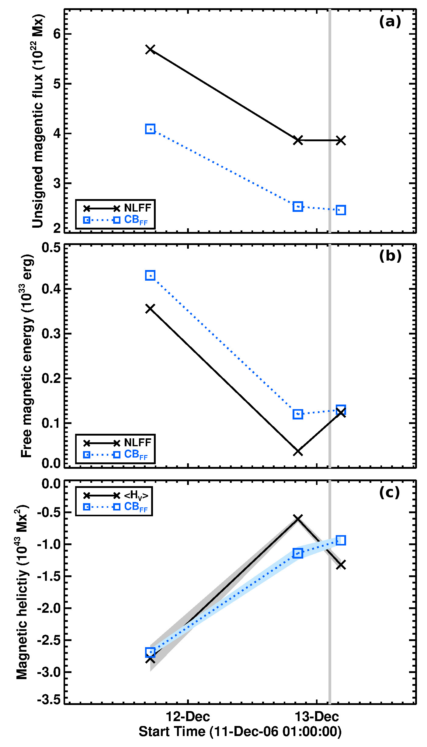
Figure 5: CB_FF calculations of the magnetic fluxes, energies and relative helicities for NOAA AR 10930 during 2006 December 11–13. (a) Total unsigned connected flux ($\phi_{c}$; blue squares) and CFIT_sc lower boundary flux (black crosses). (b) CB_FF (squares) and CFIT_sc (crosses) estimates of the free magnetic energy. (c) Mean FV ($\langle\mathscr{H}_{\mathcal{V}}\rangle$; crosses) and CB_FF (squares) relative helicities. Adjacent gray- and blue-shaded areas mark the corresponding uncertainties. The vertical gray-shaded band indicates the impulsive phase of the X3.4 flare.

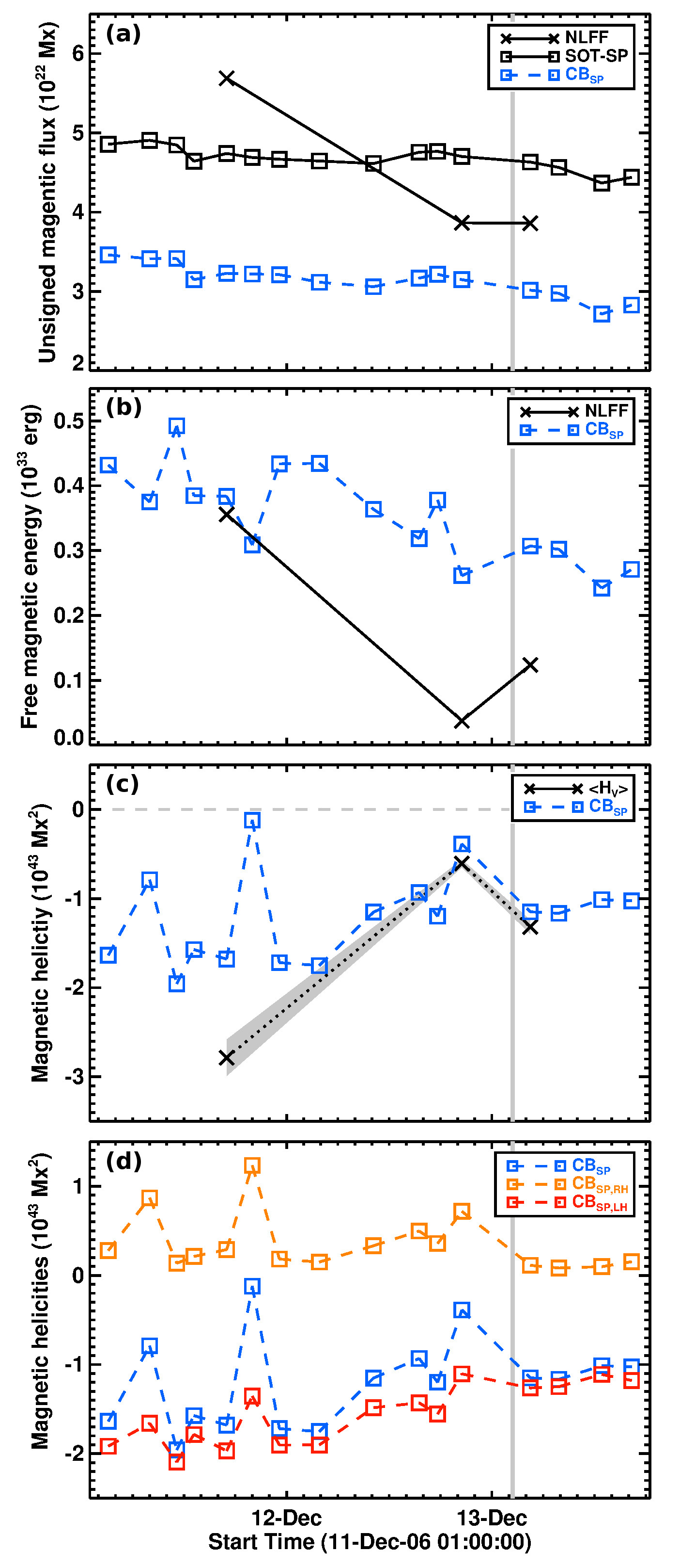
Figure 6: CB_SP calculations of the magnetic fluxes, energies and relative helicities for NOAA AR 10930 during 2006 December 11–13. (a) Total unsigned flux of SOT-SP data (black squares), total connected flux ($\phi_{c}$; blue squares), and CFIT_sc lower boundary flux (black crosses). (b) CB_SP (squares) and CFIT_sc (crosses) estimates of the free magnetic energy. (c) Mean FV ($\langle\mathscr{H}_{\mathcal{V}}\rangle$; crosses) and CB_SP (squares) relative helicities. (d) Contributions of ${\mathscr{H}}_{\rm CB,LH}$ (red) and ${\mathscr{H}}_{\rm CB,RH}$ (orange) to the CB_SP relative helicity (blue). The vertical gray-shaded band indicates the impulsive phase of the X3.4 flare.

4.3.2 Application to SOT-SP data

We show the physical quantities deduced from the CB_SP computations in Fig. 6 (for individual values see Table LABEL:tab:cbsp_detailed), in comparison to the FV estimates presented in Sect. 4.1 and Sect. 4.2.1. Let us clarify at this point that application of the CB method to 16 available SOT-SP vector magnetograms covers also the three time instances of the CB_FF application described in Sect. 4.3.1. We remind the reader here that the SP data of this section have been prepared differently (for details see Sect. 2.3) than those for the FV (hence, CB_FF) computations, including differences in linear size (field of view), spatial resolution, the azimuth disambiguation methodology and consideration of projection effects (for details see Table LABEL:tab:data). Thus, notable differences between the SP- and FV-based estimates, as discussed in the following, may partly be due to differences in the underlying data preparation (see corresponding notes in Sect. 4.1), on top of the generally different approximation of magnetic connectivity in the coronal volume due to the CB-method induced magnetic flux partitioning.

The total unsigned magnetic flux, $\phi$ computed from $B_{\rm z}$ of the 16 Level-2 SOT-SP magnetograms is of the order $(4\;-\;5)\times 10^{22}$ Mx during the considered time period (i.e., between 11 December $\sim$03:10 UT and 13 December $\sim$16:21 UT). It shows a weak increase between 12 December $\sim$06:00 UT and $\sim$18:00 UT, followed by a more or less steady decrease until about 13 December 12:00 UT (black squares in Fig. 6(a)). The SOT-SP unsigned magnetic flux is lower (by $\approx$17%) than that of the synthesized CFIT_sc lower boundary for the December 11 snapshot, and about 20% higher for the December 12 and 13 snapshots (compare black squares and black crosses, respectively, in Fig. 6(a)). The CB-based total connected flux, $\phi_{c}$, covers about 57%, 81% and 78% of the CFIT_sc lower boundary flux of the December 11, 12 and 13 snapshots, respectively (compare blue squares and black crosses in Fig. 6(a)).

The CB_SP computations for the total magnetic energy $E$ amount to 74.4%, 102.1% and 93.3% of the respective CFIT_sc FV estimates for the December 11, 12 and 13 snapshots, while for the potential energy $E_{\rm p}$ CB_SP values are 69.8%, 90.0% and 83.4% of the respective CFIT_sc FV estimates (cf.Tables LABEL:tab:nlff_modeling and LABEL:tab:cbsp_detailed). As a consequence, the CB_SP and CFIT_sc-based estimates of $E_{\rm F}$ agree for the December 11 snapshot (to within $\approx$7%) while little agreement is found for the other two snapshots: the CFIT_sc FV estimate of $E_{\rm F}$ amounts to 14.4% and 40.2%, respectively, for the December 12 and 13 snapshots.

At the corresponding time, the values of $\mathscr{H}_{\rm CB}$ are systematically smaller than $\langle\mathscr{H}_{\mathcal{V}}\rangle$: $|\mathscr{H}_{\rm CB}|$ amounts to 60.3%, 63.8% and 87.1% of $\langle|\mathscr{H}_{\mathcal{V}}|\rangle$, for the December 11, 12 and 13 snapshots, respectively (blue symbols in Fig. 6(c)). Taking a closer look into the contributions to $\mathscr{H}_{\rm CB}$, we find a dominant left-handed contribution (${\mathscr{H}}_{\rm CB,LH}$), with a magnitude larger by a factor of $\sim$8, than the right-handed contribution (${\mathscr{H}}_{\rm CB,RH}$) (compare red and orange plus signs, respectively, in Fig. 6(d)).

One notices a couple of outlier points for magnetic helicity $\mathscr{H}_{\rm CB}$ in Figs. 6(c) and 6(d), particularly in the second and sixth points of the time series (08:00 and 20:00 UT on December 11). These have been judged to relate with local disambiguation issues that have resulted in opposite-sign helicity contributions from these localizations. These issues affect the magnetic free energy estimates (Fig. 6(b)), as well, but not as much as the relative helicity.

4.4 Relative helicity flux

In Fig. 7(a) we show the total unsigned magnetic flux, $\phi$, computed from the calibrated NFI $B_{\rm los}$ (green curve and squares), used as an input to the computational methods, FI_YL and FI_EP for relative helicity flux estimations. On overall, the unsigned fluxes of the calibrated NFI data agree with that computed from the SP data to within 15%, and agree with the CFIT_sc lower boundary fluxes to within 23%, 20%, and 9%, for the 11 December 17:00 UT, 12 December 20:30 UT and 13 December 04:30 UT snapshots, respectively.

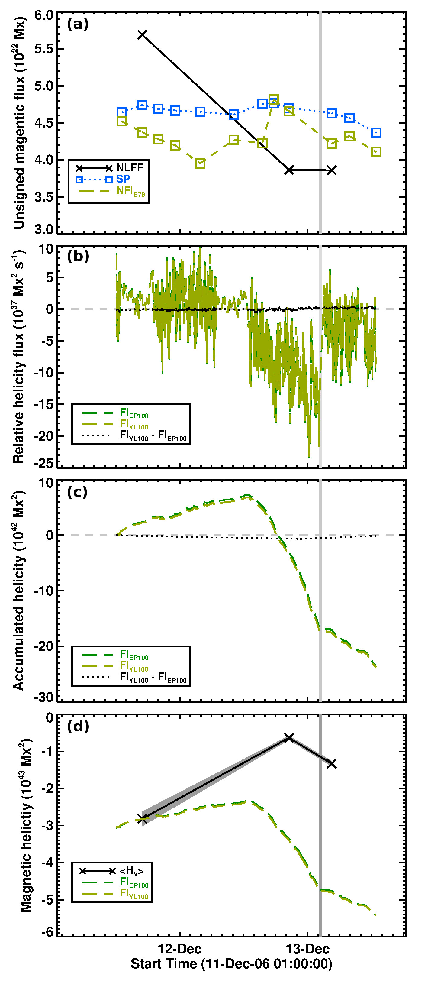
Figure 7: Magnetic and (accumulated) helicity fluxes during the interval 11 December 12:14 UT – 13 December 12:53 UT. (a) Unsigned magnetic fluxes computed from the calibrated NFI (green), SP (blue), and CFIT_sc lower boundary (black) data. (b) Relative helicity fluxes computed from the calibrated NFI data. FI_YL and FI_EP computations are represented by dark and light green color, respectively. Their signed difference is indicated by a black curve. (c) Total accumulated helicity fluxes, $H_{\mathcal{V},\rm acc}$, and corresponding signed difference. (d) Mean coronal relative helicity, $\langle\mathscr{H}_{\mathcal{V}}\rangle$, (black crosses) and theoretical curves for $H_{\mathcal{V},\rm acc}$ when using the mean estimate of $\langle\mathscr{H}_{\mathcal{V}}\rangle$ on December 11 as a reference level. The vertical gray-shaded band indicates the impulsive phase of the X3.4 flare.

Temporal profiles of the calculated helicity flux are shown in Fig. 7(b) during the same three-day interval of December 11 – 13. The helicity fluxes computed from the FI_EP and FI_YL methods, based on a threshold of 100 G for $B_{\rm z}$ (represented by light and dark green curves, respectively, and labeled FI_EP100 and FI_YL100, respectively), result in very similar values (their signed difference is shown as a black dotted line), with an agreement to within $\approx$5% (when considering all time instances when the unsigned helicity flux exceeds $1\times 10^{37}$ Mx² s^-1). Thus, the estimations of the relative helicity fluxes is largely consistent when computed by the FI_EP and FI_YL methods. Though not shown explicitly, we note here that the repetition of the FI_YL helicity flux computation using a threshold of 20 G for $B_{\rm z}$, yields helicity fluxes larger by $\approx$0.3%, in comparison to the FI_YL100 computations. This demonstrates that the helicity flux is mainly provided by the more intense magnetic polarities.

Overall, the period between 11 December $\sim$12:00 UT and 12 December $\sim$12:00 UT was characterized by a predominantly positive rate of photospheric magnetic helicity injection. The helicity injection rate appears to be rather constant around $\approx 2\times 10^{37}$ Mx² s^-1. The second half of December 12 is characterized by a transition to strong negative values, roughly centered around $-10\times 10^{37}$ Mx² s^-1. This is followed by a transition to smaller negative values early on December 13, roughly around $-2.5\times 10^{37}$ Mx² s^-1.

By time integration of the helicity fluxes, without using a reference value for the coronal helicity as a starting value, we deduce the accumulated helicity $H_{\mathcal{V},\rm acc}$ as a function of time (Fig. 7(c)), and find different trends during distinct episodes. From both, the FI_YL100 and FI_EP100 computations (the signed difference between the two is shown as a black curve), we find that $H_{\mathcal{V},\rm acc}$ steadily increases, reaching peak values of $\approx 7\times 10^{42}$ Mx² at 12 December $\sim$12:38 UT. Afterwards, $H_{\mathcal{V},\rm acc}$ decreases to negative values of $\approx-17\times 10^{42}$ Mx² at 13 December $\sim$02:13 UT (i.e., prior to flare onset), and further decreases to $\approx-24\times 10^{42}$ Mx² until 13 December $\sim$12:48 UT.

From the FI_YL100 (FI_EP100) computations, we estimate that a total of $-23.7\times 10^{42}$ Mx²($-23.6\times 10^{42}$ Mx²) was injected through the photospheric boundary for the considered time period 11 December 12:09:20 UT – 13 December 12:59:41 UT. We thus find that FI_YL and FI_EP estimation on $H_{\mathcal{V},\rm acc}$ are agreeing to within $\approx$8%. For completeness, we note that using a 20 G threshold instead of 100 G only changes the precision of the FI_YL computation of $H_{\mathcal{V},\rm acc}$ by $\approx$0.4%.

Using our mean FV-based estimate for the total helicity on 11 December 17:00 UT as a reference, so that $H_{\mathcal{V},\rm acc}=\langle\mathscr{H}_{\mathcal{V}}\rangle$ at that time instant (see intersection of green dashed and black solid line in Fig. 7(d)), we construct a hypothetical time profile, $H_{\mathcal{V},\rm acc}^{\prime}$. The values obtained for $H_{\mathcal{V},\rm acc}^{\prime}$ (dark and light green solid lines) are qualitatively different from that of the FV-based $\langle\mathscr{H}_{\mathcal{V}}\rangle$ (black solid line). More precisely, $|H_{\mathcal{V},\rm acc}^{\prime}|$ exceeds $\langle|\mathscr{H}_{\mathcal{V}}|\rangle$ by a factor of $\sim$5.4 and $\sim$3.6 for the December 12 and  13 snapshots (marked by black crosses), respectively.

The FI methods, based on the analysis of more than 1150 magnetograms, naturally provides a more detailed description of the dynamic evolution of coronal helicity than the FV-based estimates (due to the coarse time resolution of the latter). Though we find $\langle|\mathscr{H}_{\mathcal{V}}|\rangle$ to be smallest for the December 12 snapshot, the cadence of the underlying CFIT_sc models is too coarse as to allow us to assume with confidence that it represents a true peak in the time evolution of the coronal helicity. However, looking at the overall trends, we observe some qualitative agreement between the FV and the FI estimation: a decrease of negative helicity during the period spanning the second half of December 11 and the first half of December 12 and an increase in negative helicity after 12 December 20:30 UT. Quantitatively, we note a variation of $|\Delta H_{\mathcal{V},\rm acc}^{\prime}|\approx 6.8\times 10^{42}$ Mx² ($7.2\times 10^{42}$ Mx²) from the FI_YL and FI_EP computations, respectively, between 11 December $\sim$12:09 UT and 12 December $\sim$12:38 UT, which is $\approx 3$ times less than the variation of $\langle|\mathscr{H}_{\mathcal{V}}|\rangle$ during the same time span ($\approx 2.1\times 10^{43}$ Mx²). Between 12 December 12:38 UT and 13 December 04:30 UT, $|H_{\mathcal{V},\rm acc}^{\prime}|$ shows a variation of $2.4\times 10^{43}$ Mx²  while $\langle|\mathscr{H}_{\mathcal{V}}|\rangle$ varies by $\approx 0.2\times 10^{43}$ Mx², i.e., about 10 times less. Hence, while the FI and the FV methods show a partial agreement in terms of the time evolution of the coronal helicity, they quantitatively differ by several factors in the present application to observed data. Such large difference between the FI and FV methods was not observed in application to synthetic data (Pariat et al., 2021).

5 Discussion – Method comparison

In this study, we obtain the instantaneous coronal magnetic helicity budget from several FV helicity computation methods (Thalmann et al., 2011; Valori et al., 2012; Moraitis et al., 2014) relying on various NLFF field extrapolations and its approximation from the CB method (Georgoulis et al., 2012), in comparison with the accumulated magnetic helicity derived from selected FI methods (Pariat et al., 2005; Liu & Schuck, 2012). Based on high-quality (i.e., Level-2) photospheric Hinode/SOT-SP vector magnetic field observations, in combination with CFIT_sc magnetic field modeling (Wheatland & Régnier, 2009; Wheatland & Leka, 2011), we study the coronal magnetic energy and helicity of solar active region NOAA AR 10930 around an eruptive X3.4 flare (SOL2006-12-13T02:14). In the following, we discuss the main findings in regard to our main research objective, namely the cross-validation of different helicity computation methods.

5.1 Comparison of FV results

Sect. 4.2 presents the results of FV methods when applied to real solar data. Given the high solenoidality of the NLFF fields used, assessed by the normalized fraction of the energy $E_{\rm div}$ associated with magnetic monopoles (see Appendix B.1), we do not expect a strong effect on helicity values because of such artifacts. The reader is also referred to dedicated analyses on solar applications by Thalmann et al. (2019a, 2020).

As already noted by Valori et al. (2016), the accuracy of the FV helicity computed by different methods appears to be not directly related to the accuracy of the vector potentials in reproducing the corresponding fields. More precisely, the Coulomb_JT method has a lower accuracy in solving for the vector potentials than the Coulomb_SY and the DeVore methods (cf. Table LABEL:tab:fv_methods_detailed), yet it delivers similar total ($\mathscr{H}_{\mathcal{V}}$) and decomposed helicities ($\mathscr{H}_{\mathcal{V},JP}$ and $\mathscr{H}_{\mathcal{V},J}$).

Overall, the results from the different FV methods differ by $\lesssim 10.0\%$ from the common mean value, $\langle\mathscr{H}_{\mathcal{V}}\rangle$, when applied to the three CFIT_sc models (Fig. 3(a)). The same is true for the decomposed helicities (Fig. 3(b,c)) and intensive (normalized) measures (Fig. 4). These findings thus verify and complement the results of Valori et al. (2016) and Thalmann et al. (2019a, b), allowing us to assume with further confidence that FV methods provide consistent results on the local (i.e., active-region scale) coronal helicity content based on observational photospheric magnetic field data and the corresponding NLFF-extrapolated coronal magnetic fields.

5.2 Comparison of FV and CB results

In Sect. 4.3, the CB-based results have been compared to $\langle\mathscr{H}_{\mathcal{V}}\rangle$, the latter assumed to represent the “ground-truth reference value” of coronal helicity. This comparison between the CB and FV methods is by necessity limited to the estimated magnetic helicity and energy budgets since the CB method does not provide or utilize the vector potentials and reference fields.

By design, the CB method considers only a fraction of the total unsigned flux (via the connected flux $\phi_{c}$) of the supplied input data (in the form of $B_{\rm z}$ at the CFIT_sc lower boundary of the SP measurements). The extent to which magnetic information of the lower boundary is incorporated in the CB computations, however, does not seem to translate directly to a stronger or weaker agreement with FV-based values of $\langle\mathscr{H}_{\mathcal{V}}\rangle$. As an example, while $\phi_{c}$ is very similar for the December 12 and 13 snapshots for each method (both in terms of values and in terms of fraction to the total unsigned flux; see Fig. 5(a) and relevant discussion), the CB_FF helicity is $\sim 70$% of $\langle\mathscr{H}_{\mathcal{V}}\rangle$ for the December 13 snapshot and $\sim 187$% of $\langle\mathscr{H}_{\mathcal{V}}\rangle$ for the December 12 snapshot. On the contrary, despite a significantly higher $\phi_{c}$ on December 11, the helicity estimates still match to within $\approx$4% (see Fig. 5(c)).

That implies, first, a non-linearity in the differences between CB- and FV-based helicity values even given a similar amount of $\phi_{c}$ and, second, that the match between CB- and FV-based helicities might not be necessarily better in case $\phi_{c}$ better matches the total unsigned magnetic flux. This may relate to the ’arch-like’ magnetic-loops assumption of the CB method, which ignores intertwining of flux tubes in the corona because it does not require the essentially unknown full three-dimensional coronal field. This may include missing helicity contributions of both signs, thus giving rise to a nonlinear effect in the comparison.

Another nonlinear effect appears in the free magnetic energy, in which the contribution by missing braided coronal connections is always positive. Perhaps surprisingly, the CB-based estimates of the free energy are systematically larger than those based on the CFIT_sc models, by factors of 1.2, 3.0 and 1.08, respectively (Fig. 5(b)). While it is clear that $E_{\rm F,CB}$ is an underestimation of the true magnetic free energy in the corona, its systematic excess of $E_{\rm F}$ values may imply that the NLFF field extrapolations give rise to relatively smooth magnetic fields, closer to a potential-field solution than the true field.

The above said, the CB_FF and CFIT_sc results in both, free energy and helicity, are not more than a factor of three different (a factor of $\lesssim$2 for the helicity), agree in helicity sign, and provide a roughly similar evolution of the studied NOAA AR 10930, in showing a decrease of the magnetic free energy and helicity budgets between December 11 and December 13. In order words, both describe a gradual relaxation of the magnetic structure in the active region. We elaborate on this physical evolution in more detail in Sect. 6.

Overall agreements regarding FV- and CB-based estimates of the instantaneous coronal energy and helicity budgets can be found by comparison of other independently performed analyses. For instance, Tziotziou et al. (2013) and Thalmann et al. (2019b) independently studied the long-term evolution of AR 11158, showing an overall agreement of the time profiles deduced from application of the CB and a FV method, respectively (see their Figures 2e and 3b, respectively). The fact that the absolute CB_SP-based estimates are a factor of two higher than corresponding FV-based estimates may be due to several reasons, including differences in the spatial resolution of the underlying magnetic vector data and the considered FOV. This said, the overall increasing trends of helicity and free energy can be found in both studies. In another application by Patsourakos et al. (2016), the coronal helicity budget timely around a pair of X-class flares triggered in AR 11429 was studied, revealing that the CB and a FV method agree in the sense of helicity recovered (a predominantly left-handed structure), with a factor of $\sim$2 difference in helicity amplitudes (see their Table 2).

Our analysis of the CB-based helicities in Sect. 4.3.2 also shows differences between the same method (CB) when applied to SP data differing in spatial resolution, field of view (yet encompassing the essential central part of the active region), and particular steps taken in data preparation (disambiguation method and/or additional embedding in case of the CB_FF computations). While the CB_FF and CB_SP results agree qualitatively in terms of trends describing the physical evolution of the active region, it is difficult to disentangle the different quantitative effects without additional tests. This testing is left for a dedicated future work.

5.3 Comparison of FV, CB and FI results

From application of the two tested FI methods to a high-cadence time series of NFI $B_{\rm los}$ magnetic field data (Sect. 4.4), we find strong agreement between the FI_YL and FI_EP methods, to within ($\approx$8%) $\approx$5% regarding the (accumulated) helicity flux, when using the same thresholds on the level above which values of $B_{\rm los}$ are considered for FI computations. This is fully consistent with the results of Pariat et al. (2021), where a similarly good agreement between the FI_YL and FI_EP methods was found when applied to different synthetic data produced by 3D numerical simulations of solar-like events. Furthermore, when varying the threshold of $B_{\rm los}$, we find the FI_YL-based estimates of the helicity flux and accumulated helicity to agree within $\approx$0.3% and $\approx$0.4%, respectively, indicating the particular threshold used not to play a crucial role, i.e., suggesting that it is mostly the intense magnetic field area that contributes to the helicity budget.

Taking the FV-based mean estimate of the coronal helicity budget for 11 December 17:00 UT as a reference, i.e., $H_{\mathcal{V},\rm acc}=\langle\mathscr{H}_{\mathcal{V}}\rangle$ at that time instant, the relative helicity accumulation, $H_{\mathcal{V},\rm acc}^{\prime}$, suggests a decrease of the coronal helicity budget during the first half of the pre-eruption phase (between 11 December 17:00 UT and 12 December 12:38 UT) of about $|\Delta H_{\mathcal{V},\rm acc}^{\prime}|=0.5\text{--}0.6\times 10^{43}$ Mx²(Fig. 7(d)). This is quite consistent with the decrease in coronal helicity during the same period as estimated from the CB_SP computations ($|\Delta\mathscr{H}_{\rm CB}|\approx 0.7\times 10^{43}$ Mx²; compare Fig. 6(c)), but is less consistent with the overall trend seen in the FV- and CB_FF-based total helicity, the latter suggesting the corresponding decrease in coronal helicity to be larger by a factor of $\approx$3 and $\approx$2, respectively (compare Figures 3(a) and 5(c)), respectively).

In this study, however, the absolute values obtained for $H_{\mathcal{V},\rm acc}^{\prime}$ (constructed using $\langle\mathscr{H}_{\mathcal{V}}\rangle$ at 11 December 17:00 UT as a reference level) are quite different from FV-based mean estimate, $\langle|\mathscr{H}_{\mathcal{V}}|\rangle$, the latter recovering only $\approx$19% and $\approx$28% of $|H_{\mathcal{V},\rm acc}^{\prime}|$ for the December 12 and 13 snapshots, respectively (see Fig. 7(d)). This weak agreement (to within $\lesssim 30\%$ only, also observed in context with the corresponding CB-based estimates) is in line with the lack of correspondence between FV- and FI-based helicity estimates found in other applications (see e.g., Zhang et al., 2008; Park et al., 2010), but contrasts the findings based on controlled experiments, carried out by Pariat et al. (2021), which showed a good correspondence (at least to within $80\%$).

In principle, difference between FV and FI measurements are expected for flare-induced changes to the coronal helicity budget because, in contrast to FV computations, the FI methods are unlikely capable of tracking the amount of helicity carried away by a CME and the associated reorganisation of helicity within the coronal domain. This was also supported by Pariat et al. (2021), who reported strong deviations of the different helicity measures during the eruptive phase. Nevertheless, in our study, the FI-based time evolution of the coronal helicity between the pre-flare (at 12 December 20:30 UT) and post-flare (at 13 December 04:30 UT) corona appears consistent, indicating an increase of coronal helicity. We find, in particular, $|\Delta H_{\mathcal{V},\rm acc}^{\prime}|\simeq 1.4\times 10^{43}$ Mx², in comparison to $|\Delta\langle\mathscr{H}_{\mathcal{V}}\rangle|\simeq 0.71\times 10^{43}$ Mx², i.e., an agreement to within $\approx$50%.

Overall agreements regarding CB- and FI-based estimates of the instantaneous helicity budget have been demonstrated in Patsourakos et al. (2016) in their analysis of AR 11429 on 2012 March 7. In that study, the two helicity calculation methods agreed in a predominant left-handed (negative) helicity in the AR, but with a magnitude differing by a factor of $\sim$8 (see their Table 2). Surprisingly, in Patsourakos et al. (2016) the FI method gave by far the largest helicity estimate, with $H_{\mathcal{V},\rm acc}$ also by a factor of $\sim$4 larger than a corresponding FV computation.

6 Extended discussion – Physical interpretation

Our rather extensive analysis of NOAA AR 10930 affords us a picture of the complicated events that preceded the eruptive X3.4 flare, starting about 1.5 days prior to the event. In the following, we interpret our main findings in regards of the SOL2006-12-13T02:14X3.4 eruption, as well as of the active region evolution that led to it, and place them into context with existing literature.

6.1 Pre-flare evolution

We find that the interval 11 December $\sim$12:00 UT – 12 December $\sim$13:00 UT was characterized by a predominantly right-handed (positive) rate of magnetic helicity injection through the photosphere (Fig. 7(b)). This resulted in an accumulation of $H_{\mathcal{V},\rm acc}\simeq 6.8\times 10^{42}$ Mx² of positive helicity in the corona (Fig. 7(c)). Afterwards, the rate of helicity injection transited to strong negative values, persisting until just before the time of the X-class flare on December 13 and resulting in a total of $H_{\mathcal{V},\rm acc}\approx 17\times 10^{42}$ Mx² in left-handed (negative) helicity at 20:30 UT on December 12. Excluding the FI-based estimates during the nominal flare duration, we find a further increase of the total accumulated coronal helicity budget until the end of the investigated time period at 13 December $\sim$12:00 UT, amounting to a total of $H_{\mathcal{V},\rm acc}=-23.7\times 10^{42}$ Mx² during the entire analysis interval.

Notice that our estimates of the (accumulated) helicity flux are roughly an order of magnitude larger than those in earlier studies (e.g., Zhang et al., 2008; Park et al., 2010). From those studies, and taking our estimate of $\langle\mathscr{H}_{\mathcal{V}}\rangle$ as a reference, one would conclude that $H_{\mathcal{V},\rm acc}$ accounted for only a minor contribution to the coronal helicity budget. Instead, we find in this study that $H_{\mathcal{V},\rm acc}$ contributes markedly and evolves only partly consistently in time with the FV-based estimates. We attribute the discrepancy between our results and those published earlier to the challenge of proper data calibration, i.e., the quality of the photospheric magnetic field data used to carry out the helicity flux computations. In short, only when omitting any calibration of the NFI data, we are able to reproduce the (accumulated) helicity fluxes of, e.g., Zhang et al. (2008) and Park et al. (2010). Given the strong difference between the results obtained with or without calibration (cf. Appendix A.1), our study points to the care requested when handling the input magnetic field data in order to properly use the FI methods with observed data.

From our analysis of individual contributions to volumetric estimates (Fig. 3), a clear dominance of the volume-threading helicity ($\mathscr{H}_{\mathcal{V},JP}$) is recovered, being about an order of magnitude larger than the current-carrying helicity ($\mathscr{H}_{\mathcal{V},J}$). Corresponding dominant contributions of $\mathscr{H}_{\mathcal{V},JP}$ are known from earlier simulation-based (e.g., Pariat et al., 2017; Zuccarello et al., 2018; Linan et al., 2018) and observation-based (James et al., 2018; Moraitis et al., 2019; Thalmann et al., 2019b; Price et al., 2019) works. Yet puzzling are our estimates of the helicity ratio ($|\mathscr{H}_{\mathcal{V},J}|/|\mathscr{H}_{\mathcal{V}}|$; Fig. 4(b)). From observational studies of individual ARs prolific in eruptive X-class flares, pre-flare peak values of $\gtrsim$0.15 were found (e.g., Moraitis et al., 2019; Thalmann et al., 2019b). The comparative recent work by Gupta et al. (2021), in which ten different ARs are studied, places these values to an extreme, with CME-productive ARs showing characteristic pre-flare values of $\gtrsim$0.1. In sharp contrast, we find a corresponding mean FV-based pre-flare estimate of $<$0.1 (Fig. 4(b)), which might be related to our NLFF models being more potential (with $E_{\rm F}/E\lesssim 0.1$) than in earlier studies of CME-productive ARs.

The time evolution of $\langle\mathscr{H}_{\mathcal{V}}\rangle$ suggests a decrease of the coronal helicity budget during December 12. Quantitatively, we find the total helicity to decrease between 11 December 17:00 UT and 12 December 20:30 UT by $2.2\times 10^{42}$ Mx² (see Fig. 3(a)), in overall agreement with the decrease in coronal helicity evaluated by Park et al. (2010) (see their Fig. 1) and Georgoulis et al. (2012) (see their Fig. 7a) during the same time period. From the CB_SP computations (Fig. 6(d)), one notices a dominant left-handed contribution (${\mathscr{H}}_{\rm CB,LH}$) decreasing during the same period, consistent with the assumption of an magnetic configuration of negative overall helicity. A co-temporal weak increase of the corresponding right-handed contribution (${\mathscr{H}}_{\rm CB,RH}$), however, suggests the emergence of an oppositely helical (i.e., right-handed) magnetic structure, consistent with our finding of a positive helicity flux discussed above.

Overall, the above described trends support a scenario of a right-handed structure emerging into a pre-existing, predominantly left-handed magnetic configuration during December 11 and the first half of December 12. This is consistent with the NLFF model-based findings of Inoue et al. (2012) who showed that the active-region magnetic field was predominantly negatively twisted about one day prior to the X-class flare, as well as the formation of positively twisted field near the polarity inversion line prior to flare onset. Consistently, we recover a positively sheared arcade from our CFIT_sc models. A system of strong electric currents is found in the arch filament system on December 11 17:00 UT and an associated low-lying sheared arcade connecting the two main sunspots on December 12 at 20:30 UT (Fig. 2(b)).

6.2 Pre- and post-flare conditions in comparison

A complicated, challenging picture also appears in comparing pre- and post-flare configurations in regards to the major, GOES X3.4 flare in the active region over the studied interval.

First, we interpret a sign reversal in the photospheric helicity flux during the impulsive phase of the flare to be nonphysical, contrary to earlier studies (e.g., Zhang et al., 2008; Park et al., 2010; Ravindra et al., 2011). In those studies, it was suggested to represent a signature of the rapid emergence of a magnetic structure of opposite handedness, possibly responsible for the triggering of the flare. In our study, however, we present support that helicity flux estimates during this particular flare lack realism, and excluded those during the nominal flare duration from analysis (for details see Appendix A.2). Consequently, we question the interpretation of a sudden and impulsive helicity injection as the trigger of the X3.4 flare, and refer to LaBonte et al. (2007) and Xu et al. (2018) for the discussion of better observed, and more credible, flare-related changes.

Second, from our FV and CB_SP computations, we find an increase in the coronal helicity between 12 December 20:30 UT and 13 December 04:30 UT of $|\Delta\langle\mathscr{H}_{\mathcal{V}}\rangle|\simeq 0.71\times 10^{43}$ Mx² and $\simeq$$0.76\times 10^{43}$ Mx², respectively, in line with earlier works (e.g., Park et al., 2010; Georgoulis et al., 2012). Since our FV-based decomposition of the total helicity allows it, we find the differences between the pre-flare and post-flare snapshots to be more pronounced in the volume-threading ($\mathscr{H}_{\mathcal{V},JP}$) than in the current-carrying ($\mathscr{H}_{\mathcal{V},J}$) helicities ($\approx$11% vs. $\approx$6%, respectively, of the pre-flare value of $\langle\mathscr{H}_{\mathcal{V}}\rangle$), and more pronounced in the right-handed (${\mathscr{H}}_{\rm CB,RH}$) than the left-handed (${\mathscr{H}}_{\rm CB,LH}$) contribution to $\mathscr{H}_{\rm CB}$ ($\approx 56\%$ vs. $\approx 41\%$ of the pre-flare $\mathscr{H}_{\rm CB}$, respectively). Thus, we may assume with relative confidence that $\mathscr{H}_{\mathcal{V},J}$ (showing a flare-related increase, as does ${\mathscr{H}}_{\rm CB,LH}$) is dominated by the core (left-handed) field in the active region, left behind after the ejection of a previously emerged right-handed structure.

Third, based on our CFIT_sc magnetic field models, we find the free magnetic energy ($E_{\rm F}$) to be higher for the post-flare configuration (Table LABEL:tab:nlff_modeling). From our volumetric estimates on 12 December 20:30 UT and 13 December 04:30 UT, we quantify the corresponding increase as to be $\Delta E_{\rm F}\approx 1\times 10^{32}$ erg. Also the fraction of $E_{\rm F}$ compared to the total energy is higher in the post-flare corona ($\approx$6%, compared to $\approx$2% for the pre-flare corona). This increasing trend is in line with the results obtained from 13 out of 14 NLFF solutions compared in Schrijver et al. (2008), and is in line with the findings of Jing et al. (2008) regarding the increase of magnetic shear in the course of the flare.

Consistent increasing trends are found from the CB_FF (Table LABEL:tab:cbff_modeling and Fig. 5(b)) and CB_SP (Table LABEL:tab:cbsp_detailed and Fig. 6(b)) results, suggesting however an increase of $E_{\rm F}$ by a factor of eight and two lower than the CFIT_sc-based estimates, respectively. Regardless, these findings contradict those of other studies. The ${\rm Wh}_{\rm pp}^{+}$ NLFF modeling reported in Schrijver et al. (2008), suggests a flare-related decrease of $\Delta E_{\rm F}\approx 3\times 10^{32}$ erg, in loose agreement (about an order of magnitude higher) with the corresponding estimate of Guo et al. (2008). Being necessarily related to the differing pre-flare magnetic topology recovered from our CFIT_sc modeling, the discrepancy regarding the recovered time evolution of the coronal magnetic energies may again be attributed to the overall uncertainties and ambiguity of NLFF modeling.

7 Summary

The study and analysis presented herein serves the primary purpose of cross-validating different calculation methods of the relative magnetic helicity in the well-studied AR 10930 around the time of an eruptive major flare (SOL2006-12-13T02:14X3.4). It is part of a series of ISSI-supported studies devoted to comparisons between the results of different helicity calculation methods (Valori et al., 2016; Guo et al., 2017; Pariat et al., 2021) and is the first study of the series employing solar observations.

To the above objective, we used the following helicity calculation methods:

• Five different finite volume (FV) methods (cf. Sect. 3.1), relying on the classical volume-integral magnetic helicity formula, applied to a series of three NLFF field extrapolations (CFIT_sc; cf. Sect. 2.2). The CFIT_sc modeling used a synthetic photospheric boundary, constructed from Hinode SOT-SP vector magnetograms and SOHO/MDI LOS magnetograms (Sect. 2.1).

• The connectivity-based (CB) method, relying on a partitioning of photospheric magnetic flux distributions (Sect. 3.2), applied to two different sets of photospheric boundary data: once to the CFIT_sc lower boundary vector magnetic field (CB_FF), and once to a time series of 16 Level-2 SOT-SP vector magnetograms (CB_SP).

• Two different helicity-flux integration (FI) methods (Sect. 3.3), relying on a high-cadence time series of 1150 Hinode SOT-NFI LOS magnetograms (FI_YL and FI_EP methods).

The FV and CB methods provide instantaneous budgets of the magnetic free energy ($E_{\rm F}$) and relative helicity ($\mathscr{H}_{\mathcal{V}}$) in the active-region corona, while the FI methods provide the helicity injection rate through the photosphere and an accumulated (i.e., time-integrated) helicity ($H_{\mathcal{V},\rm acc}$) thereof.

In regards of our main research objective, namely the cross-validation of different methods, we found a number of promising aspects:

• A close correspondence between FV estimates, both in extensive and intensive estimates, with an agreement to within a few percent.

• Agreement on the dominant (left-handed) helicity in the AR as deduced from the FV and CB methods.
  Overall agreement between FV- and CB-based estimates regarding recovered time trends, deemed as remarkable given the very different settings of the methods: the CB method only models the coronal magnetic connectivity while the FV methods requires it as an explicit input.

• A close correspondence between FI estimates, with an agreement to within a few percent.

• Overall agreement between FV- and FI-based estimates regarding the predominant sign and magnitude of the coronal helicity. This is also deemed as remarkable, given that the FI method only capture the flux of helicity supplied to the corona via the photosphere.

In terms of the second objective, namely the interpretation of the active region evolution that led to the SOL2006-12-13T02:14X3.4 eruption, we found an overall decreasing free magnetic energy and relative magnetic helicity during 2006 December 11 – 12, and increased values for the post-flare corona on December 13. All FV, CB_FF and CB_SP results basically corroborate this picture, with the CB_SP method further implying the possible expulsion of an oppositely helical (i.e., right-handed) structure in the course of the eruption that was previously embedded (and, possibly, emerged during the previous 24 hours) into a predominantly left-handed magnetic configuration.

In this analysis, furthermore, we encountered and identified a number of significant caveats:

• Our CFIT_sc model results are significantly different than the best-performing (${\rm Wh}_{\rm pp}^{+}$) NLFF model in the community-supported study of Schrijver et al. (2008), even to the point of leading to different physical interpretations. Our results allow interpretations in line with 13 out of 14 NLFF models analyzed in that work (and also in line with Jing et al., 2008), pointing at the long-known uncertainties and ambiguities of NLFF modeling.

• Our CFIT_sc models do not show a coronal flux rope being present in the pre-flare corona (a highly sheared arcade instead). Studies advocating for the pre-flare existence of flux ropes exist (e.g., Gibson et al., 2006), while recent reviews advocate for an evolutionary course from an initial sheared magnetic arcade to a magnetic flux rope during the eruption (Georgoulis et al., 2019; Patsourakos et al., 2020, and references therein).

• Our interpretation of a possible ejection of an oppositely helical magnetic structure stands in agreement with some modeling works (e.g., Inoue et al., 2012) but disagrees with others (e.g., Fan, 2016) that modeled an ejected helical structure with like (i.e., left-) handedness to the prevailing helicity sense in the active region.

• For the FV and CB methods, photospheric boundary conditions are crucial to the quantitative results. Nevertheless, the match of the FV-based estimates from the CB method is apparently unrelated to the fraction of the true magnetic flux considered.

• CB_FF and CB_SP results are significantly different, relying on CFIT_sc lower boundary and original SP magnetograms, respectively.

• FI computations based on high-cadence, high-quality photospheric vector magnetograms, allow a detailed and realistic account of the helicity buildup rate in an active region, hence they critically depend on data calibration.

• Spurious signals in the FI results (showing a fast transition to helicity injection of opposite sign) during the nominal duration of the X3.4 flare, might be wrongly interpreted as representing an observational signature of a right-handed magnetic structure having impulsively emerged.

• FI computations need a reference point for the starting helicity budget to complete the evolutionary picture. Even with such a reference level at hand (e.g., via a FV-based estimate), significant discrepancies between the deduced helicity budgets may be found (up to $\approx 70\%$ in this study), lacking a sound, well-justified explanation to date.

• In terms of the free magnetic energy, CB_FF results give consistently higher values than CFIT_sc results, albeit by reasonable factors 1–3 (compare Tables LABEL:tab:nlff_modeling and LABEL:tab:cbff_modeling), despite representing a minimum coronal free energy by construction of the CB method. This points to a potential underestimation of the free energy in the corona by NLFF field extrapolations.

In brief, this study highlights the intricacies and difficulties of interpreting a complexity-ridden solar eruption by means of a quantitative data analysis of its host active region. While the X3.4-flare related eruption must have undoubtedly resulted in magnetic energy release and helicity expulsion, our results suggest enhanced respective budgets at a time shortly afterwards. One might be quick to discard these results as counter-intuitive or less credible, if only a single method to estimate the coronal energy and helicity budgets were used. The independent overall agreement by different methods in this study, however, may nudge one toward a slightly more complicated picture, namely, one of competing tendencies in the active region. Regardless how large an eruptive flare, it only releases a relatively small fraction of the free energy in the region (up to $\sim 10$%) and up to $\sim$30-40% of its helicity (e.g., Nindos et al., 2003; Gibson & Fan, 2008; Moraitis et al., 2014). Hence, tendencies of buildup or decay may well be stronger than the respective eruption budgets imposing the need for a wider investigation of active region evolution and dynamics around eruptions, rather than a mere focus on the eruptions themselves.

Appendix A Data sources and preparation

We summarize the sources and processing particular data used for NLFF modeling and/or helicity computations in Table LABEL:tab:data, including the time (range) for which data was acquired (first column), the number of snapshots considered (second column), the particular data source used (third column), as well as the plate scale of the resulting data product (fifth column). If applied, the method used for disambiguation of the magnetic field azimuth is listed in the fourth column. The remaining columns point at the places in the manuscript where the corresponding FOVs are visualized (sixth column) and explained in detail (last column).

Table A1: Data sources and preparation for CFIT_sc modeling and the application of the different helicity computation methods. Indicated from left to right are the instances or time range, where applicable, of data coverage, the number of snapshots used within the covered time range, the data source, disambiguation method (where applicable; otherwise a cross ’$\times$’ is used), the plate scale, the indication of the covered area on the solar disk in Fig. 1 (for data other than on December 11, a cross ’$\times$’ is used) and the location of detailed data description in the main document.

Time (range)	No. of	Data	Disambiguation	Plate scale	Covered area	Detailed
(UT)	snapshots	source	method	(arcsec)	as outlined in Fig. 1	description
CFITsc NLFF modeling
Dec 11 17:00	1	SOT-SPa	NPFCb	0.66	magenta outline	Sect. 2.1
Dec 12 20:30	1	SOT-SPa	MEc	0.63	$\times$	– ” –
Dec 13 04:30	1	SOT-SPa	MEc	0.63	$\times$	– ” –
FV helicity computations
Dec 11 17:00	1	CFITsc $\mathbfit{B}$	$\times$	0.66	magenta outline	Sect. 2.2
Dec 12 20:30	1	CFITsc $\mathbfit{B}$	$\times$	0.63	$\times$	– ” –
Dec 13 04:30	1	CFITsc $\mathbfit{B}$	$\times$	0.63	$\times$	– ” –
CBFF helicity computation
Dec 11 17:00	1	CFITsc $\mathbfit{B}$ at $z=0$	$\times$	0.66	magenta outline	Sects. 2.2 & 2.3
Dec 12 20:30	1	CFITsc $\mathbfit{B}$ at $z=0$	$\times$	0.63	$\times$	– ” –
Dec 13 04:30	1	CFITsc $\mathbfit{B}$ at $z=0$	$\times$	0.63	$\times$	– ” –
CBSP helcity computation
Dec 11 03:10 – Dec 13 16:21	16	SOT-SP $B_{\rm z}$	NPFCb	0.31	yellow outlinee	Sect. 2.3
FI helcity flux computation
Dec 11 12:09 – Dec 13 12:59	1150	SOT-NFId $B_{\rm los}$	$\times$	0.15	green outline	Sect. 2.4

^a https://csac.hao.ucar.edu/sp_data.php

^b Non-Potential magnetic Field Calculation (NPFC) method (Georgoulis, 2005; Metcalf et al., 2006)

^c Minimum-energy (ME) method (Metcalf, 1994; Metcalf et al., 2006)

^d Ichimoto & Hinode/SOT Team (2008)

^e For December 11 data only

A.1 Effect of NFI data calibration on FI computations

In order to compute the photospheric helicity flux, three main steps are to be undertaken: calibration of $B_{\rm los}$ (or not), inversion of flux transport velocities, and helicity flux computation. From the results presented in Sect. 5.3, we know that the helicity flux computation itself (step three above) is not a source of major discrepancies, as the retrieved (accumulated) fluxes with the FI_EP and FI_YL methods are fairly consistent.

Using the SP data as a reference Chae et al. (2007) suggest to calibrate NFI data (step one mentioned above) in the following way. In regions outside the sunspots and penumbral regions, a linear relation between the circular polarization and $B_{\rm los}$ is used (their Eq. 7). The resulting calibrated $B_{\rm los}$ (light green dashed line labeled ”B7” in Fig. A1(a)) yields total unsigned fluxes on the order of $\approx 80\%$, on average, compared to the SP flux (blue dotted line), and about 66%, 106%, and 93% of the CFIT_sc lower boundary fluxes (black crosses) on December 11, 12 and 13, respectively. Additionally, in umbral regions a first-order polynomial can be adopted in order to model the reversal of the polarization signal over field strength (their Eq. 8). The resulting calibrated $B_{\rm los}$ (dark green long-dash, labeled ”B78”) yields a total unsigned flux of $\gtrsim 85\%$, on average, in comparison to that of SP, and about 77%, 120% and 109% of the CFIT_sc lower boundary flux for the December 11, 12, and 13 snapshot, respectively. In comparison, the non-calibrated NFI data (yellow solid line) recovers only about 25% of the SP unsigned magnetic flux, on average, i.e., about 20%, 34% and 31% of the CFIT_sc lower boundary flux for the December 11, 12, and 13 snapshot.

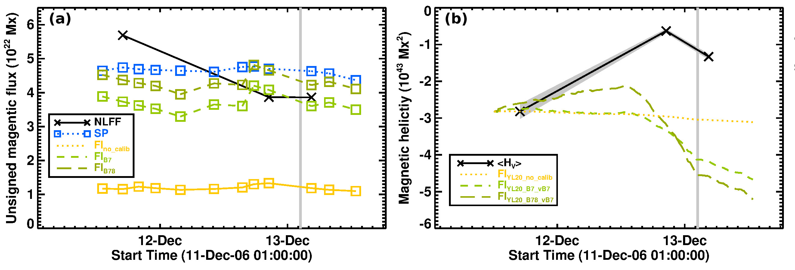
Figure A1: Magnetic and (accumulated) helicity fluxes based on different calibration products. (a) Unsigned magnetic fluxes. Estimates based on calibrated NFI $B_{\rm los}$ excluding (including) sunspot areas are shown as light green dashed (dark green long-dashed) lines, and labeled “B7” (”B78”). For comparison, fluxes based on the non-calibrated data are shown in yellow (labeled ”no_calib”), based on SP $B_{\rm z}$ in blue, and based on CFIT_sc $B_{\rm z}$ in black. (b) theoretical curve for $H_{\mathcal{V},\rm acc}$ when using the mean estimate of $\langle\mathscr{H}_{\mathcal{V}}\rangle$ on December 11 as a reference level, based on FI_YL computations (labeled “FI_YL20”), using DAVE velocities deduced from B7-data. For comparison, $\langle\mathscr{H}_{\mathcal{V}}\rangle$ is shown as black crosses (solid line). The vertical gray-shaded band indicates the impulsive phase of the X3.4 flare.

Using the non-calibrated $B_{\rm los}$ as the basis for DAVE-velocity and subsequent helicity flux computations, one obtains a predominantly negative rate of magnetic helicity injection through the photosphere during most of the considered time interval ($\propto 10^{36}$ Mx² s^-1; not shown explicitly) and the resulting accumulation of coronal helicity during the considered time period of $H_{\mathcal{V},\rm acc}=-2.9\times 10^{42}$ Mx² (see yellow dotted curve in Fig. A1(b)). Since this result, based on the non-calibrated $B_{\rm los}$, is in overall agreement with the corresponding estimates from earlier studies (e.g., Zhang et al., 2008; Park et al., 2010), we must therefore question the validity of those, as well as their interpretation. This includes, e.g., earlier conclusions on $H_{\mathcal{V},\rm acc}$ to represent only a minor contribution to the coronal helicity budget (being about an order of magnitude larger in amplitude).

In order to investigate the effect of step one (calibration of $B_{\rm los}$) to the retrieved helicity flux, we compute it based on the two aforementioned data sets (B7 and B78), using $\mathbfit{u}$ deduced using DAVE from B7. For completeness, we note here that we do not deduce DAVE flux transport velocities from the B78 data, as discontinuities spatially associated with saturation effects, yield unrealistic velocity estimates. Though not explicitly shown, we note here that the relative helicity fluxes computed from the calibrated NFI data (both, B7 and B78, with DAVE applied to the B7 data) are remarkably higher (by a factor of $\gtrsim 10$) than that based on the non-calibrated data, as is the total accumulated helicity. More precisely, we estimate a total of $H_{\mathcal{V},\rm acc}=-18.5\times 10^{42}$ Mx² and $H_{\mathcal{V},\rm acc}=-23.9\times 10^{42}$ Mx² for the considered time period, from the B7 and B78 data sets, respectively (cf. green dashed and long-dashed curves in Fig. A1(b)), respectively). Furthermore, instead of a rather flat time profile as for the non-calibrated data (yellow dotted curve in Fig. A1(b)), we find a time evolution drastically different, namely $H_{\mathcal{V},\rm acc}$ decreasing until about noon on December 12 and increasing until after the X-class flare.

A.2 Effect of data disclosure on FI computations

Careful inspection of the (non-)calibrated NFI data shows artifacts largely co-spatial with the saturated umbra, especially during the flare (see Fig. A2(a)–(d)). In particular, nonphysical DAVE velocities are retrieved from the calibrated field, that are not representative of the magnitude or direction typically found in sunspots (Fig. A2(c)–(d)). Therefore, we excluded the time range 13 December 02:14 UT – 02:57 UT (the nominal GOES flare duration) from helicity flux analysis (indicated by the dashed vertical lines in Fig. A2(e), that shows a transition from negative to positive fluxes (irrespective of the particular calibration applied).

The effect on the deduced values for the total accumulated helicity, based on the B78 data set (favored due to the reasons outlined above), is marginal. We estimate $H_{\mathcal{V},\rm acc}=-23.7\times 10^{42}$ Mx² when excluding the nominal GOES flare duration (indicated by the vertical dashed lines in Fig. A2(e)), in comparison to $H_{\mathcal{V},\rm acc}=-22.6\times 10^{42}$ Mx² without data disclosure. Obviously, the latter estimate is slightly smaller due to the transition of the sudden transition of the helicity flux to positive values during the nominal GOES flare duration.

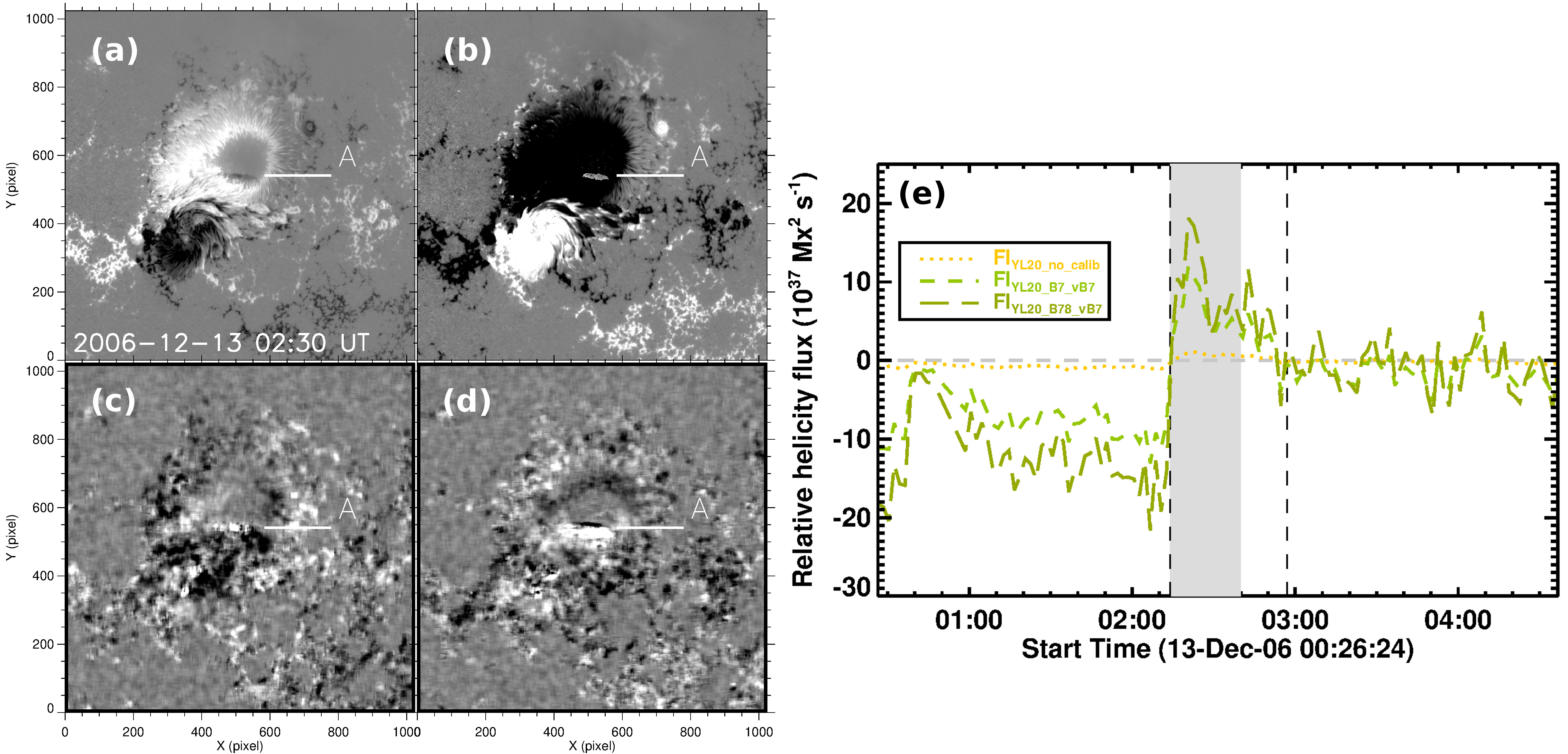
Figure A2: Magnetic field data and flux transport velocity during the flare. Calibrated NFI (a) Stokes-V and (b) $B_{\rm los}$ (B78) data. DAVE flux transport velocities, (c) $v_{x}$ and (d) $v_{y}$, saturated at $\pm 0.2$ km/s. The horizontal line labeled ”A” in (a)–(d) points at the artificial patterns observed in the umbral area. (e) Helicity flux computations around the time of the X-class flare. Estimates based on calibrated NFI $B_{\rm los}$ excluding (including) sunspot areas are shown as light green dashed (dark green long-dashed) lines, and labeled “B7” (”B78”). Helicity fluxes based on the non-calibrated data are represented by the yellow dotted line (labeled ”no_calib”). The vertical dashed lines mark the time interval which was disclosed from analysis (the nominal GOES flare duration). The vertical gray-shaded band indicates the nominal impulsive phase of the flare.

Appendix B NLFF modeling

The NLFF code CFIT (Wheatland, 2007) uses the Grad-Rubin method to solve for the coronal magnetic field, $\mathbfit{B}$, and the force-free parameter, $\alpha_{\rm ff}$, where $\mathbfit{B}$ and $\alpha_{\rm ff}$ are related through

$$\mathbfit{\nabla}\times\mathbfit{B}=\alpha_{\rm ff}\mathbfit{B}\text{\hskip 14.22636ptand\hskip 14.22636pt}\mathbfit{B}\cdot\nabla\alpha_{\rm ff}=0,$$ (B1)

As an input the method requires the vertical magnetic field component, $B_{z}$ over both magnetic polarities, and the specification of $\alpha_{\rm ff}$ over one magnetic polarity. This is equivalent to a corresponding specification of the normal component of the electric current density, $J_{z}$, since $\mathbfit{J}=\alpha_{\rm ff}\mathbfit{B}/\mu_{0}$.

CFIT solves for $\mathbfit{B}$ and $\mathbfit{J}$ iteratively, so that at the $i$th iteration

$$\mathbfit{B}^{i-1}\cdot\nabla\alpha_{\rm ff}^{i}=0\mathrm{~{}~{}~{}and~{}~{}~{}}\nabla\times\mathbfit{B}^{i}=\alpha_{\rm ff}^{i}\,\mathbfit{B}^{i-1}$$ (B2)

is solved (Wheatland, 2007). Here, given $\mathbfit{B}^{i-1}$, $\mathbfit{B}^{i}$ is solved for, subject to $\mathbfit{\nabla}\cdot\mathbfit{B}^{i}=0$, as well as the boundary conditions $\alpha_{\rm ff}^{i}$ and $B_{\rm z}^{i}$ at $z=0$. The start equilibrium, $\mathbfit{B}^{0}$, is specified by a potential field matching the boundary conditions on $B_{\rm z}$, hence implying $\mathbfit{J}^{0}=0$.

Grad-Rubin methods, however, have been found to deliver inconsistent results for NLFF reconstructions if relying on the boundary conditions on $\alpha_{\rm ff}$ specified on one magnetic polarity only; either positive or negative (Schrijver et al., 2008; DeRosa et al., 2009). In other words, two very different NLFF solutions may be obtained, given a single vector magnetogram. In order to resolve this inherent inconsistency, Wheatland & Régnier (2009) expanded the original CFIT method by a “self-consistency” procedure (“CFIT_sc”, hereafter).

The CFIT_sc method is favored in the present work because of its advantageous properties, including its strict convergence when applied to solar data, hence providing a single (average) solution to the force-free problem, as explained in the following (for more details see Wheatland & Régnier, 2009; Wheatland & Leka, 2011).

First, CFIT solutions are constructed for the boundary conditions on $\alpha_{\rm ff}$ specified once from the positive (P solution) and once from the negative (N solution) magnetic polarity field. To reduce the effects of nonphysical currents, values of $\alpha_{\rm ff}$ are used only if the signal-to-noise ratio exceeds a certain threshold and are set to zero otherwise (the so-called “censoring”). The computational volume is defined as a uniform three-dimensional Cartesian grid (i.e., solar curvature is ignored) with equal grid spacing in each dimension. The update of $\mathbfit{B}$ via Eq. (B2) is achieved by solving the Poisson equation for the corresponding vector potential using a two-dimensional Fourier Transform method, so that the solution is correspondingly periodic in $x$ and $y$. A mapping of $\alpha_{\rm ff}$ along of model field lines in the P solution then allows to define updated boundary values in the negative polarity domain, and vice versa. Consequently, the two solutions define a new set of boundary conditions on $\alpha_{\rm ff}$ over the entire vector magnetogram. Second, based on probability theory, the most probable value of $\alpha_{\rm ff}$ is determined, by averaging the values of $\alpha_{\rm ff}$, weighted by the uncertainties, from the original boundary values and those resulting from the mappings of the P and N solutions (Wheatland & Régnier, 2009). Finally, steps one and two above are iterated (self-consistency cycling), in order to obtain a self-consistent solution (for a further recent work see Mastrano et al., 2020).

B.1 Quality of the CFIT_sc models

In order to quantify the force-freeness of the obtained CFIT_sc solutions, we use the current-density-weighted (sine of the) angle between the modeled magnetic field and electric current density, ($\rm CWsin$) $\theta_{J}$, (Schrijver et al., 2006) and find values ($\lesssim 0.4$) $\lesssim 25^{\circ}$ for all CFIT_sc solutions (see last two columns in Table LABEL:tab:metrics).

In order to assess the quality of the solenoidal condition in the CFIT_sc solutions we use a measure for local derivations of solenoidality within the model volume, in the form of the volume-averaged fractional flux ($\langle\,|f_{i}(\mathbfit{B})|\,\rangle$; see Wheatland et al. (2000) and Gilchrist et al. (2020) for a most recent dedicated analysis). For all CFIT_sc models, we find $\langle\,|f_{i}(\mathbfit{B})|\,\rangle\lesssim 2.0\times 10^{-4}$ (see third-last column Table LABEL:tab:metrics).

The applicability of FV methods depends critically on how well $\mathbfit{\nabla}\cdot\mathbfit{B}=0$ and $\mathbfit{\nabla}\cdot\mathbfit{B}_{\rm p}=0$ are fulfilled. A corresponding quality measure, alternative to $\langle\,|f_{i}(\mathbfit{B})|\,\rangle$ discussed above, has been introduced by Valori et al. (2013), in the form of the ratio $E_{\rm div}/E$, where

$$E = \frac{1}{2\mu_{0}}\int_{\mathcal{V}}B^{2}\,{\rm d}\mathrm{V}=E_{\rm p}+E_{\rm J}$$ (B3)

$$= E_{\rm p,s}+E_{\rm J,s}+E_{\rm p,ns}+E_{\rm J,ns}+E_{\rm mix}.$$

Table B1: Quality metrics of the CFIT_sc NLFF fields. Columns indicate the potential solenoidal ($E_{\rm p,s}$), current-carrying solenoidal ($E_{\rm J,s}$), potential nonsolenoidal ($E_{\rm p,ns}$), current-carrying nonsolenoidal ($E_{\rm J,ns}$), and mixed nonsolenoidal ($E_{\rm mix}$) energy contributions normalized to the corresponding total energy $E$ (see respective column in Table LABEL:tab:nlff_modeling). Last columns include the average fractional flux ($\langle\,|f_{i}(\mathbfit{B})|\,\rangle$), $\theta_{J}$, and the current-weighted value of $\sin\theta_{J}$, CWsin, where $\theta_{J}$ is the average angle between $\mathbfit{B}$ and the electric current density, $\mathbfit{J}$. For a perfectly force-free solution, $\theta_{J}=0^{\circ}$.

Date & Time	$E_{\rm p,s}/E$	$E_{\rm J,s}/E$	$E_{\rm p,ns}/E$	$E_{\rm J,ns}/E$	$E_{\rm mix}/E$	$\langle\,|f_{i}(\mathbfit{B})|\,\rangle\times 10^{5}$	CWsin	$\theta_{J}[^{\circ}]$
11 Dec 17:00 UT	0.88	0.12	2.47e-04	1.82e-04	2.17e-03	18.22	0.414	24.460
12 Dec 20:30 UT	0.98	0.02	1.01e-04	7.88e-05	3.24e-05	8.93	0.380	22.354
13 Dec 04:30 UT	0.94	0.06	8.20e-05	9.56e-05	1.40e-03	8.82	0.341	19.950

Here, $E_{\rm p}$ and $E_{\rm J}$ are the energies of the potential and current-carrying magnetic field, respectively. $E_{\rm p,s}$ and $E_{\rm J,s}$ are those of the potential and current-carrying solenoidal magnetic field components, respectively, where $E_{\rm J,s}$ is the free energy in an ideal (i.e., fully solenoidal) solution. Furthermore, $E_{\rm p,ns}$ and $E_{\rm J,ns}$ are the (spurious) energies of the corresponding non-solenoidal components, and $E_{\rm mix}$ corresponds to all cross terms (see Eq. (8) in Valori et al., 2013, for the detailed expressions). Except for $E_{\rm mix}$, all contributions to Eq. (B3) are positive definite. For a perfectly solenoidal field, one finds $E_{\rm p,s}=E_{\rm p}$, $E_{\rm J,s}=E_{\rm J}$, and $E_{\rm p,ns}=E_{\rm J,ns}=E_{\rm mix}=0$. The sum of the non-solenoidal contributions to the total energy is $E_{\rm div}/E$, where $E_{\rm div}=(E_{\rm p,ns}+E_{\rm J,ns}+|E_{\rm mix}|)$.

In the proof-of-concept study by Valori et al. (2016), based on solar-like numerical experiments, it was suggested that only for input fields achieving $E_{\rm div}/E\lesssim 0.1$ a reliable helicity computation may be expected. Dedicated follow-up studies suggested an even lower threshold for solar applications ($E_{\rm div}/E\lesssim 0.05$; Thalmann et al., 2019a), necessarily related to minimal non-solenoidal contributions to the free magnetic energy ($|E_{\rm mix}|/E_{\rm J,s}\lesssim 0.4$; Thalmann et al., 2020). In the present work, all considered NLFF fields have a solenoidal level well below these thresholds, with $E_{\rm div}/E<0.01$ and $|E_{\rm mix}|/E_{\rm J,s}<0.1$ (cf. numbers listed in Table LABEL:tab:metrics). Thus, we may assume a correspondingly small error in the helicity computations.

Furthermore, based on the energy decomposition above, we find that the CFIT_sc model magnetic fields on December 12 and 13 are found closer to a potential field state than that on December 11, as revealed by the relatively higher values of $E_{\rm p,s}/E$ in Table LABEL:tab:metrics.

Appendix C (Accuracy of) FV and CB helicities

We list the relative helicities computed by the different FV methods (based on the CFIT_sc solutions described in Sect. 2.2) in Table LABEL:tab:fv_methods_detailed. The accuracy with which the vector potentials $\mathbfit{A}$ and $\mathbfit{A}_{\rm p}$ reproduce the respective input magnetic field, $\mathbfit{B}$ and $\mathbfit{B}_{\rm p}$, are listed for each of the considered FV methods in Table LABEL:tab:ei_hi. The physical quantities deduced from the CB_SP computations, i.e. the CB method applied to the 16 available SOT-SP vector magnetograms described in Sect. 2.3, are displayed in Table LABEL:tab:cbsp_detailed.

Table C1: FV computations. Relative helicities $\mathscr{H}_{\mathcal{V}}$, $\mathscr{H}_{\mathcal{V},J}$, and $\mathscr{H}_{\mathcal{V},JP}$ obtained from four individual FV helicity computation methods (see Sect. 3.1) are given in units of $10^{43}$ Mx².

Method (as in	Date & Time	Relative helicities			Intensive quantities
Sect. 3.1 and Table LABEL:tab:methods)		$\mathscr{H}_{\mathcal{V}}$	$\mathscr{H}_{\mathcal{V},J}$	$\mathscr{H}_{\mathcal{V},JP}$	$\tilde{\mathscr{H}}_{\mathcal{V}}$	$|\mathscr{H}_{\mathcal{V},J}|/|\mathscr{H}_{\mathcal{V}}|$
Coulomb_JT	11 Dec 17:00 UT	-3.1472	-0.2626	-1.8847	-0.0389	0.0834
Coulomb_JT	12 Dec 20:30 UT	-0.6780	-0.0040	-0.6741	-0.0182	0.0058
Coulomb_JT	13 Dec 04:30 UT	-1.4449	-0.0405	-1.4043	-0.0388	0.0281
Coulomb_SY	11 Dec 17:00 UT	-2.6896	-0.2634	-2.4263	-0.0332	0.0979
Coulomb_SY	12 Dec 20:30 UT	-0.5832	-0.0049	-0.5783	-0.0156	0.0083
Coulomb_SY	13 Dec 04:30 UT	-1.2693	-0.0417	-1.2276	-0.0341	0.0328
DeVore_KM	11 Dec 17:00 UT	-2.6993	-0.2633	-2.4360	-0.0334	0.0975
DeVore_KM	12 Dec 20:30 UT	-0.6116	-0.0051	-0.6065	-0.0164	0.0084
DeVore_KM	13 Dec 04:30 UT	-1.3354	-0.0437	-1.2917	-0.0359	0.0327
DeVore_GV	11 Dec 17:00 UT	-2.6912	-0.2629	-2.4283	-0.0333	0.0977
DeVore_GV	12 Dec 20:30 UT	-0.5817	-0.0046	-0.5771	-0.0156	0.0079
DeVore_GV	13 Dec 04:30 UT	-1.2701	-0.0416	-1.2285	-0.0341	0.0327
DeVore_SA	11 Dec 17:00 UT	-2.6993	-0.2635	-2.4358	-0.0334	0.0976
DeVore_SA	12 Dec 20:30 UT	-0.5847	-0.0049	-0.5798	-0.0156	0.0084
DeVore_SA	13 Dec 04:30 UT	-1.2751	-0.0417	-1.2334	-0.0342	0.0327

Table C2: Metrics of accuracy of vector potentials in reproducing the corresponding magnetic field. $C_{\rm Vec}$ is the vector correlation, analogous to the standard correlation coefficient for scalar functions. If two vector fields are identical, then $C_{\rm Vec}=1$. $C_{\rm CS}$ is a measure of the angular differences of the vector fields. For parallel fields, $C_{\rm CS}=1$, and is $-1$ for anti-parallel fields. $\epsilon_{\rm N}$ and $\epsilon_{\rm M}$ are the complements of the normalized and mean vector error, respectively. $\epsilon_{\rm E}$ gives the energy ratio, i.e., the ratio of the total energy with respect to the input field. For the computation of these metrics the standard numerical prescriptions as described in Appendix A of Valori et al. (2013) were applied.

Method (as in	Date & Time	$\mathbfit{B}_{\rm p}$ vs $\mathbfit{\nabla}\times\mathbfit{A}_{\rm p}$					$\mathbfit{B}$ vs $\mathbfit{\nabla}\times\mathbfit{A}$
Sect. 3.1 and Table LABEL:tab:methods)		$C_{\rm Vec}$	$C_{\rm CS}$	$\epsilon_{\rm N}$	$\epsilon_{\rm M}$	$\epsilon_{\rm E}$	$C_{\rm Vec}$	$C_{\rm CS}$	$\epsilon_{\rm N}$	$\epsilon_{\rm M}$	$\epsilon_{\rm E}$
Coulomb_JT	11 Dec 17:00 UT	0.6685	0.6283	0.0058	-0.6641	2.2166	0.6909	0.6473	0.0693	-0.6612	2.0819
Coulomb_JT	12 Dec 20:30 UT	0.6429	0.6163	-0.1707	-0.7033	2.4263	0.6461	0.6182	-0.1667	-0.7059	2.4118
Coulomb_JT	13 Dec 04:30 UT	0.6339	0.6150	-0.1860	-0.7055	2.4841	0.6451	0.6251	-0.1604	-0.7105	2.4053
Coulomb_SY	11 Dec 17:00 UT	0.9996	0.9990	0.9758	0.9604	1.0011	0.9995	0.9987	0.9738	0.9552	0.9985
Coulomb_SY	12 Dec 20:30 UT	0.9995	0.9992	0.9724	0.9594	1.0011	0.9995	0.9988	0.9681	0.9523	1.0005
Coulomb_SY	13 Dec 04:30 UT	0.9995	0.9992	0.9722	0.9595	1.0011	0.9995	0.9988	0.9686	0.9525	0.9992
DeVore_KM	11 Dec 17:00 UT	0.9999	1.0000	0.9985	0.9995	0.9994	0.9998	1.0000	0.9981	0.9994	0.9995
DeVore_KM	12 Dec 20:30 UT	0.9999	1.0000	0.9536	0.9533	1.0885	0.9999	1.0000	0.9535	0.9533	1.0887
DeVore_KM	13 Dec 04:30 UT	0.9999	1.0000	0.9536	0.9533	1.0887	0.9998	1.0000	0.9534	0.9533	1.0889
DeVore_GV	11 Dec 17:00 UT	0.9999	1.0000	0.9981	0.9990	0.9980	1.0000	1.0000	0.9987	0.9995	0.9987
DeVore_GV	12 Dec 20:30 UT	1.0000	1.0000	0.9986	0.9990	0.9985	1.0000	1.0000	0.9991	0.9997	0.9990
DeVore_GV	13 Dec 04:30 UT	1.0000	1.0000	0.9987	0.9991	0.9985	1.0000	1.0000	0.9992	0.9997	0.9990
DeVore_SA	11 Dec 17:00 UT	0.9999	1.0000	0.9988	0.9996	1.0004	0.9999	1.0000	0.9982	0.9994	0.9995
DeVore_SA	12 Dec 20:30 UT	1.0000	1.0000	0.9993	0.9998	1.0002	1.0000	1.0000	0.9989	0.9996	0.9998
DeVore_SA	13 Dec 04:30 UT	1.0000	1.0000	0.9993	0.9998	1.0002	0.9999	1.0000	0.9989	0.9996	0.9995

Table C3: CB_SP results. Unsigned magnetic flux ($\phi$), total connected flux ($\phi_{c}$), relative helicity ($\mathscr{H}_{\rm CB}$) and corresponding error ($\Delta{\mathscr{H}}_{\rm CB,LH}$), right-handed helicity (${\mathscr{H}}_{\rm CB,RH}$) and corresponding error ($\Delta{\mathscr{H}}_{\rm CB,RH}$), left-handed helicity (${\mathscr{H}}_{\rm CB,LH}$) and corresponding error ($\Delta{\mathscr{H}}_{\rm CB,LH}$), total ($E$) and potential ($E_{\rm p}$) magnetic energy, along with error $\Delta E$ in $E$. Magnetic fluxes are given in units of $10^{22}$ Mx, energies in units of $10^{33}$ erg, and helicities in units of $10^{43}$ Mx².

Date & Time	Magnetic fluxes		Relative helicities						Magnetic energies
	$\phi$	$\phi_{c}$	$\mathscr{H}_{\rm CB}$	$\Delta\mathscr{H}_{\rm CB}$	${\mathscr{H}}_{\rm CB,RH}$	$\Delta{\mathscr{H}}_{\rm CB,RH}$	${\mathscr{H}}_{\rm CB,LH}$	$\Delta{\mathscr{H}}_{\rm CB,LH}$	$E$	$\Delta E$	$E_{\rm p}$
				($\times 10^{-2}$)		($\times 10^{-2}$)		($\times 10^{-2}$)		($\times 10^{-3}$)
11 Dec 03:10:04	4.8571	3.460	-1.6366	1.8668	0.2794	1.0956	-1.9159	1.5115	2.2773	4.3920	1.8455
11 Dec 08:00:04	4.9060	3.412	-0.7902	4.1563	0.8691	2.5952	-1.6593	3.2465	2.2166	5.1245	1.8415
11 Dec 11:10:06	4.8468	3.416	-1.9559	1.6046	0.1362	0.5837	-2.0921	1.4946	2.3332	4.5147	1.8410
11 Dec 13:10:09	4.6428	3.148	-1.5726	2.0504	0.2121	1.0199	-1.7847	1.7788	2.1877	4.3450	1.8031
11 Dec 17:00:08	4.7401	3.228	-1.6789	2.8096	0.2889	1.3113	-1.9679	2.4848	2.2087	5.4217	1.8251
11 Dec 20:00:05	4.6891	3.220	-0.1214	4.6167	1.2331	3.0320	-1.3546	3.4815	2.1001	6.1313	1.7914
11 Dec 23:10:05	4.6676	3.212	-1.7192	1.7963	0.1828	0.7172	-1.9020	1.6470	2.2220	4.3465	1.7884
12 Dec 03:50:05	4.6455	3.116	-1.7519	1.7362	0.1495	0.6102	-1.9015	1.6255	2.2010	4.2237	1.7664
12 Dec 10:10:08	4.6140	3.060	-1.1519	2.5019	0.3321	1.0915	-1.4840	2.2513	2.0862	4.9743	1.7227
12 Dec 15:30:08	4.7559	3.168	-0.9320	3.8538	0.4975	2.2275	-1.4295	3.1448	2.0300	4.9267	1.7116
12 Dec 17:40:05	4.7669	3.216	-1.1977	2.3044	0.3575	1.3592	-1.5552	1.8609	2.0813	4.4163	1.7034
12 Dec 20:30:05	4.7015	3.148	-0.3878	3.6809	0.7175	2.8076	-1.1053	2.3803	1.9293	4.6931	1.6680
13 Dec 04:30:05	4.6319	3.016	-1.1493	1.1832	0.1131	0.5406	-1.2624	1.0525	1.9230	3.9054	1.6160
13 Dec 07:50:05	4.5646	2.976	-1.1658	1.0349	0.0827	0.3717	-1.2485	0.9659	1.8930	4.0902	1.5910
13 Dec 12:51:04	4.3675	2.716	-1.0129	1.1522	0.0978	0.3922	-1.1107	1.0834	1.7029	3.3812	1.4607
13 Dec 16:21:04	4.4393	2.828	-1.0250	1.1816	0.1537	0.6383	-1.1786	0.9943	1.7662	3.9294	1.4953

References

- Berger (1984) Berger, M. A. 1984, Geophysical and Astrophysical Fluid Dynamics, 30, 79, doi: 10.1080/03091928408210078
- Berger (1999) —. 1999, Plasma Physics and Controlled Fusion, 41, B167, doi: 10.1088/0741-3335/41/12B/312
- Berger & Field (1984) Berger, M. A., & Field, G. B. 1984, Journal of Fluid Mechanics, 147, 133, doi: 10.1017/S0022112084002019
- Cargill (2009) Cargill, P. J. 2009, Space Sci. Rev., 144, 413, doi: 10.1007/s11214-008-9446-9
- Chae et al. (2007) Chae, J., Moon, Y.-J., Park, Y.-D., et al. 2007, PASJ, 59, S619, doi: 10.1093/pasj/59.sp3.S619
- Démoulin (2007) Démoulin, P. 2007, Advances in Space Research, 39, 1674, doi: 10.1016/j.asr.2006.12.037
- Démoulin & Berger (2003) Démoulin, P., & Berger, M. A. 2003, Sol. Phys., 215, 203, doi: 10.1023/A:1025679813955
- Démoulin & Pariat (2009) Démoulin, P., & Pariat, E. 2009, Advances in Space Research, 43, 1013, doi: 10.1016/j.asr.2008.12.004
- Demoulin et al. (2006) Demoulin, P., Pariat, E., & Berger, M. A. 2006, Sol. Phys., 233, 3, doi: 10.1007/s11207-006-0010-z
- DeRosa et al. (2009) DeRosa, M. L., Schrijver, C. J., Barnes, G., et al. 2009, ApJ, 696, 1780, doi: 10.1088/0004-637X/696/2/1780
- DeRosa et al. (2015) DeRosa, M. L., Wheatland, M. S., Leka, K. D., et al. 2015, ApJ, 811, 107, doi: 10.1088/0004-637X/811/2/107
- Fan (2011) Fan, Y. 2011, ApJ, 740, 68, doi: 10.1088/0004-637X/740/2/68
- Fan (2016) —. 2016, ApJ, 824, 93, doi: 10.3847/0004-637X/824/2/93
- Finn & Antonsen (1985) Finn, J. M., & Antonsen, T. M. 1985, Comm. Plasma Phys. Control. Fusion, 9, 111
- Georgoulis (2005) Georgoulis, M. K. 2005, ApJ, 629, L69, doi: 10.1086/444376
- Georgoulis & LaBonte (2007) Georgoulis, M. K., & LaBonte, B. J. 2007, ApJ, 671, 1034, doi: 10.1086/521417
- Georgoulis et al. (2019) Georgoulis, M. K., Nindos, A., & Zhang, H. 2019, Philosophical Transactions of the Royal Society of London Series A, 377, 20180094, doi: 10.1098/rsta.2018.0094
- Georgoulis et al. (2012) Georgoulis, M. K., Tziotziou, K., & Raouafi, N.-E. 2012, ApJ, 759, 1, doi: 10.1088/0004-637X/759/1/1
- Gibson & Fan (2008) Gibson, S. E., & Fan, Y. 2008, Journal of Geophysical Research (Space Physics), 113, A09103, doi: 10.1029/2008JA013151
- Gibson et al. (2006) Gibson, S. E., Fan, Y., Török, T., & Kliem, B. 2006, Space Sci. Rev., 124, 131, doi: 10.1007/s11214-006-9101-2
- Gilchrist et al. (2020) Gilchrist, S. A., Leka, K. D., Barnes, G., Wheatland , M. S., & DeRosa, M. L. 2020, arXiv e-prints, arXiv:2008.08863. https://arxiv.org/abs/2008.08863
- Guo et al. (2013) Guo, Y., Ding, M. D., Cheng, X., Zhao, J., & Pariat, E. 2013, ApJ, 779, 157, doi: 10.1088/0004-637X/779/2/157
- Guo et al. (2010) Guo, Y., Ding, M. D., Schmieder, B., et al. 2010, ApJ, 725, L38, doi: 10.1088/2041-8205/725/1/L38
- Guo et al. (2008) Guo, Y., Ding, M. D., Wiegelmann, T., & Li, H. 2008, ApJ, 679, 1629, doi: 10.1086/587684
- Guo et al. (2017) Guo, Y., Pariat, E., Valori, G., et al. 2017, ApJ, 840, 40, doi: 10.3847/1538-4357/aa6aa8
- Gupta et al. (2021) Gupta, M., Thalmann, J. K., & Veronig, A. M. 2021, A&A, accepted
- Ichimoto & Hinode/SOT Team (2008) Ichimoto, K., & Hinode/SOT Team. 2008, Plasma and Fusion Research, 2, 1009, doi: 10.1585/pfr.2.S1009
- Inoue et al. (2012) Inoue, S., Shiota, D., Yamamoto, T. T., et al. 2012, ApJ, 760, 17, doi: 10.1088/0004-637X/760/1/17
- James et al. (2018) James, A. W., Valori, G., Green, L. M., et al. 2018, ApJ, 855, L16, doi: 10.3847/2041-8213/aab15d
- Jing et al. (2008) Jing, J., Wiegelmann, T., Suematsu, Y., Kubo, M., & Wang, H. 2008, ApJ, 676, L81, doi: 10.1086/587058
- Kosugi et al. (2007) Kosugi, T., Matsuzaki, K., Sakao, T., et al. 2007, Sol. Phys., 243, 3, doi: 10.1007/s11207-007-9014-6
- LaBonte et al. (2007) LaBonte, B. J., Georgoulis, M. K., & Rust, D. M. 2007, ApJ, 671, 955, doi: 10.1086/522682
- Linan et al. (2018) Linan, L., Pariat, É., Moraitis, K., Valori, G., & Leake, J. 2018, ApJ, 865, 52, doi: 10.3847/1538-4357/aadae7
- Lites et al. (2007) Lites, B., Casini, R., Garcia, J., & Socas-Navarro, H. 2007, Mem. Soc. Astron. Italiana, 78, 148
- Lites et al. (2013) Lites, B. W., Akin, D. L., Card, G., et al. 2013, Sol. Phys., 283, 579, doi: 10.1007/s11207-012-0206-3
- Liu & Schuck (2012) Liu, Y., & Schuck, P. W. 2012, The Astrophysical Journal, 761, 105, doi: 10.1088/0004-637X/761/2/105
- Low (1994) Low, B. C. 1994, Physics of Plasmas, 1, 1684, doi: 10.1063/1.870671
- Mastrano et al. (2020) Mastrano, A., Yang, K. E., & Wheatland, M. S. 2020, Sol. Phys., 295, 97, doi: 10.1007/s11207-020-01663-7
- Metcalf (1994) Metcalf, T. R. 1994, Sol. Phys., 155, 235, doi: 10.1007/BF00680593
- Metcalf et al. (2006) Metcalf, T. R., Leka, K. D., Barnes, G., et al. 2006, Sol. Phys., 237, 267, doi: 10.1007/s11207-006-0170-x
- Moffatt (1969) Moffatt, H. K. 1969, Journal of Fluid Mechanics, 35, 117, doi: 10.1017/S0022112069000991
- Moraitis et al. (2019) Moraitis, K., Sun, X., Pariat, É., & Linan, L. 2019, A&A, 628, A50, doi: 10.1051/0004-6361/201935870
- Moraitis et al. (2014) Moraitis, K., Tziotziou, K., Georgoulis, M. K., & Archontis, V. 2014, Sol. Phys., 289, 4453, doi: 10.1007/s11207-014-0590-y
- Nindos et al. (2003) Nindos, A., Zhang, J., & Zhang, H. 2003, ApJ, 594, 1033, doi: 10.1086/377126
- Pariat et al. (2005) Pariat, E., Démoulin, P., & Berger, M. A. 2005, Astronomy and Astrophysics, 439, 1191, doi: 10.1051/0004-6361:20052663
- Pariat et al. (2017) Pariat, E., Leake, J. E., Valori, G., et al. 2017, A&A, 601, A125, doi: 10.1051/0004-6361/201630043
- Pariat et al. (2015) Pariat, E., Valori, G., Démoulin, P., & Dalmasse, K. 2015, A&A, 580, A128, doi: 10.1051/0004-6361/201525811
- Pariat et al. (2021) Pariat, E., Valori, G., Anfinogentov, S., et al. 2021, Space Sci. Rev., in preparation
- Park et al. (2010) Park, S.-H., Chae, J., Jing, J., Tan, C., & Wang, H. 2010, ApJ, 720, 1102, doi: 10.1088/0004-637X/720/2/1102
- Patsourakos et al. (2016) Patsourakos, S., Georgoulis, M. K., Vourlidas, A., et al. 2016, ApJ, 817, 14, doi: 10.3847/0004-637X/817/1/14
- Patsourakos et al. (2020) Patsourakos, S., Vourlidas, A., Török, T., et al. 2020, Space Sci. Rev., 216, 131, doi: 10.1007/s11214-020-00757-9
- Price et al. (2019) Price, D. J., Pomoell, J., Lumme, E., & Kilpua, E. K. J. 2019, A&A, 628, A114, doi: 10.1051/0004-6361/201935535
- Priest (2014) Priest, E. 2014, Magnetohydrodynamics of the Sun (Cambridge University Press), doi: 10.1017/CBO9781139020732
- Ravindra et al. (2011) Ravindra, B., Venkatakrishnan, P., Tiwari, S. K., & Bhattacharyya, R. 2011, ApJ, 740, 19, doi: 10.1088/0004-637X/740/1/19
- Rust (1994) Rust, D. M. 1994, Geophys. Res. Lett., 21, 241, doi: 10.1029/94GL00003
- Scherrer et al. (1995) Scherrer, P. H., Bogart, R. S., Bush, R. I., et al. 1995, Sol. Phys., 162, 129, doi: 10.1007/BF00733429
- Schrijver et al. (2006) Schrijver, C. J., De Rosa, M. L., Metcalf, T. R., et al. 2006, Sol. Phys., 235, 161, doi: 10.1007/s11207-006-0068-7
- Schrijver et al. (2008) Schrijver, C. J., De Rosa, M. L., Metcalf, T., et al. 2008, ApJ, 675, 1637, doi: 10.1086/527413
- Schuck (2006) Schuck, P. W. 2006, ApJ, 646, 1358, doi: 10.1086/505015
- Schuck (2008) —. 2008, ApJ, 683, 1134, doi: 10.1086/589434
- Thalmann et al. (2011) Thalmann, J. K., Inhester, B., & Wiegelmann, T. 2011, Sol. Phys., 272, 243, doi: 10.1007/s11207-011-9826-2
- Thalmann et al. (2019a) Thalmann, J. K., Linan, L., Pariat, E., & Valori, G. 2019a, ApJ, 880, L6, doi: 10.3847/2041-8213/ab2e73
- Thalmann et al. (2019b) Thalmann, J. K., Moraitis, K., Linan, L., et al. 2019b, ApJ, 887, 64, doi: 10.3847/1538-4357/ab4e15
- Thalmann et al. (2020) Thalmann, J. K., Sun, X., Moraitis, K., & Gupta, M. 2020, A&A, 643, A153, doi: 10.1051/0004-6361/202038921
- Titov & Démoulin (1999) Titov, V. S., & Démoulin, P. 1999, A&A, 351, 707
- Tsuneta et al. (2008) Tsuneta, S., Ichimoto, K., Katsukawa, Y., et al. 2008, Sol. Phys., 249, 167, doi: 10.1007/s11207-008-9174-z
- Tziotziou et al. (2013) Tziotziou, K., Georgoulis, M. K., & Liu, Y. 2013, ApJ, 772, 115, doi: 10.1088/0004-637X/772/2/115
- Valori et al. (2012) Valori, G., Démoulin, P., & Pariat, E. 2012, Sol. Phys., 278, 347, doi: 10.1007/s11207-012-9951-6
- Valori et al. (2013) Valori, G., Démoulin, P., Pariat, E., & Masson, S. 2013, A&A, 553, A38, doi: 10.1051/0004-6361/201220982
- Valori et al. (2016) Valori, G., Pariat, E., Anfinogentov, S., et al. 2016, Space Sci. Rev., 201, 147, doi: 10.1007/s11214-016-0299-3
- Welsch et al. (2007) Welsch, B. T., Abbett, W. P., De Rosa, M. L., et al. 2007, The Astrophysical Journal, 670, 1434, doi: 10.1086/522422
- Wheatland (2007) Wheatland, M. S. 2007, Sol. Phys., 245, 251, doi: 10.1007/s11207-007-9054-y
- Wheatland & Leka (2011) Wheatland, M. S., & Leka, K. D. 2011, ApJ, 728, 112, doi: 10.1088/0004-637X/728/2/112
- Wheatland & Régnier (2009) Wheatland, M. S., & Régnier, S. 2009, ApJ, 700, L88, doi: 10.1088/0004-637X/700/2/L88
- Wheatland et al. (2000) Wheatland, M. S., Sturrock, P. A., & Roumeliotis, G. 2000, ApJ, 540, 1150, doi: 10.1086/309355
- Wiegelmann et al. (2017) Wiegelmann, T., Petrie, G. J. D., & Riley, P. 2017, Space Sci. Rev., 210, 249, doi: 10.1007/s11214-015-0178-3
- Wiegelmann & Sakurai (2012) Wiegelmann, T., & Sakurai, T. 2012, Living Reviews in Solar Physics, 9, 5, doi: 10.12942/lrsp-2012-5
- Xu et al. (2018) Xu, Y., Cao, W., Ahn, K., et al. 2018, Nature Communications, 9, 46, doi: 10.1038/s41467-017-02509-w
- Yang et al. (2020) Yang, K. E., Wheatland, M. S., & Gilchrist, S. A. 2020, ApJ, 894, 151, doi: 10.3847/1538-4357/ab8810
- Yang et al. (2013) Yang, S., Büchner, J., Santos, J. C., & Zhang, H. 2013, Sol. Phys., 283, 369, doi: 10.1007/s11207-013-0236-5
- Yang et al. (2018) Yang, S., Büchner, J., Skála, J., & Zhang, H. 2018, A&A, 613, A27, doi: 10.1051/0004-6361/201628108
- Zhang et al. (2008) Zhang, Y., Tan, B., & Yan, Y. 2008, ApJ, 682, L133, doi: 10.1086/591027
- Zuccarello et al. (2018) Zuccarello, F. P., Pariat, E., Valori, G., & Linan, L. 2018, ApJ, 863, 41, doi: 10.3847/1538-4357/aacdfc