Jeans instability in an expanding universe with dissipation

Abstract

Jeans instability is analysed in an expanding universe within the framework of BGK model of the Boltzmann equation and Poisson equations. The background is characterized by a comoving Maxwellian distribution function and a space-time Newtonian gravitational potential which satisfy the BGK model of the Boltzmann and Poisson equations without the necessity to invoke ”Jeans swindle”. The perturbations of the distribution function and Newtonian gravitational potentials from their background states are represented by plane waves of small amplitudes and a differential equation for the density contrast is determined. The density contrast differential equation was solved numerically and it is shown: (i) Jeans instability is characterized by perturbation wavelengths larger than Jeans wavelength where the density contrast grows with time. The growth of the density contrast is less accentuated for the case where the particle collisions are considered due to an energy dissipation; (ii) for perturbation wavelengths smaller than Jeans wavelength the density contrast has an oscillatory behavior in time and the oscillations for the case where the collisions are taken into account fade away in time due to the energy dissipation.

I Introduction

The determination of the instabilities of self-gravitating fluids from the hydrodynamic equations of mass and momentum densities coupled with the Newtonian Poisson equation is an old subject in the literature. It was first analyzed by Jeans [1] in 1902 who determined a wavelength cutoff from a dispersion relation – known nowadays as Jeans wavelength. – where the perturbations may propagate as harmonic waves in time for wavelengths smaller than the Jeans wavelength or may grow or decay in time for larger wavelengths. The Jeans instability refers to the gravitational collapse of self-gravitating interstellar gas clouds associated with the mass density perturbations which grow exponentially with time [2, 3, 4]. Physically a mass density inhomogeneity collapses when the outwards pressure force is smaller than the inwards gravitational force.

The analysis of Jeans instability in an expanding Universe by considering the Newtonian hydrodynamic equations coupled with the Newtonian Poisson equation was due to Bonnor [5] in 1957. This problem is also described in the books [2, 3]. We call attention to the fact that the Newtonian gravity is still valid in regions whose radius are small compared with the Hubble radius and the velocities are non-relativistic.

One can also investigate the Jeans instability within the framework of the collisionless Boltzmann equation coupled with the Newtonian Poisson equation (see e.g [3, 4, 6, 7, 8, 9, 10, 11, 12]).

If one considers the collision term in the Boltzmann equation irreversible processes related to the dissipative effects of viscosity and heat conductivity show up. Hence to take into account dissipative effects in the analysis of the Jeans instability one has to consider the collisional Boltzmann equation. Within the framework of a collisional Boltzmann equation Jeans instability was first analyzed in [13]. Another methodology to take into account the dissipaitve effects is to consider the hydrodynamic equations for a viscous and heat conducting fluid which was recently analyzed in [14].

The aim of the present work is to analyse the Jeans instability from the collisional Boltzmann equation coupled with the Newtonian Poisson equation in an expanding Universe ruled by a spatially flat Friedmann-Lamaître-Robertson-Walker (FLRW) metric. Here the BGK model of the Boltzmann equation is consider for the collision term.

The background distribution function is characterized by a comoving Maxwellian distribution function which satisfies identically the BGK model of the Boltzmann equation. The background Newtonian gravitational potential satisfies the Poisson equation without the necessity to invoke ”Jeans swindle”. The perturbed one-particle distribution function and Newtonian gravitational potential from their background states are represented by plane waves of small amplitudes. Furthermore, the perturbed amplitude of the distribution function is consider as a function of the summational invariants [9, 11, 12]. A differential equation for the density contrast is obtained from the system of differential equations for the amplitudes. The numerically solutions of the differential equation shown that: (i) for perturbation wavelengths larger than Jeans wavelength the density contrast grows with time which characterizes Jeans instability. The growth of the density contrast is less accentuated for the case where the particle collisions are considered due to an energy dissipation; (ii) for perturbation wavelengths smaller than Jeans wavelength the density contrast has an oscillatory behavior in time. The oscillations for the case where the collisions are taken into account fade away in time due to the energy dissipation.

The paper is structured as follows. In Section II the the background solution is analyzed. The Jeans instability is determined in Section III where the perturbed solution is investigated. The conclusions are given in Section IV.

II Analysis of the background solution

The Boltzmann equation describes the space-time evolution of the one-particle distribution function $f(\mathbf{x},\mathbf{v},t)$ in the phase space spanned by the spatial coordinates $\mathbf{x}$ and velocity $\mathbf{v}$ of the particles. In the non-relativistic framework it reads (see e.g. [15])

$$\frac{\partial f}{\partial t}+v_{i}\frac{\partial f}{\partial x^{i}}+\frac{\partial f}{\partial v_{i}}\frac{\partial U}{\partial x^{i}}=\mathcal{Q}(f,f).$$ (1)

Here $\mathcal{Q}(f,f)$ is the collision operator of the Boltzmann equation which is given by the product of the distribution functions of two particles at binary collisions.

The Boltzmann equation (1) is linked with the Poisson equation for the Newtonian gravitational potential $U$, namely

$$\nabla^{2}U=-4\pi G\rho=-4\pi G\int mfd^{3}v,$$ (2)

where $G$ denotes the universal gravitational constant and $\rho$ the mass density of the fluid. Above the mass density is given in terms of the one-particle distribution function where $m$ denotes the particle rest mass.

In this work we shall consider the BGK model of the Boltzmann equation where the structure of the collision operator is simplified but preserves the basic properties of the full Boltzmann equation (see e.g. [15]). The collision operator in the BGK model is given in terms of the difference between the one-particle distribution function $f$ and the equilibrium Maxwellian distribution function $f_{0}$ multiplied by a frequency $\nu$ which is of order of the collision frequency. The BGK model of the Boltzmann equation reads

$$\frac{\partial f}{\partial t}+v_{i}\frac{\partial f}{\partial x^{i}}+\frac{\partial U}{\partial x^{i}}\frac{\partial f}{\partial v^{i}}=-\nu(f-f_{0}).$$ (3)

Here we are interested in investigating the Jeans instability in an expanding Universe which is ruled by the spatially flat Friedmann-Lamaître-Robertson-Walker (FLRW) metric $ds^{2}=(cdt)^{2}-a(t)(dx^{2}+dy^{2}+dz^{2})$, where $a(t)$ is the cosmic scale factor.

In a comoving frame the Maxwellian distribution function is written as

$$f_{0}(\mathbf{v},t)=\frac{\rho(t)}{m}\frac{1}{[2\pi\sigma(t)^{2}]^{3/2}}\exp\left[-\frac{\left(\mathbf{v}-\dot{a}\mathbf{x}_{0}\right)^{2}}{2\sigma(t)^{2}}\right],$$ (4)

by taking into account the Hubble-Lamaître’s law ${\bf x}(t)=a(t){\mathbf{x}_{0}}$, which relates the comoving coordinates $\mathbf{x}_{0}$ with the physical coordinates $\bf x$. The Maxwellian distribution function (4) – which is considered as the background distribution function – depends on the fluid mass density $\rho(t)$ and dispersion velocity $\sigma(t)$ which are functions of time.

The dependence of the background mass density on time is determined from Friedmann equations, which for a pressureless fluid is given by

$$\rho(t)=\rho_{0}\left(\frac{a_{0}}{a(t)}\right)^{3},\qquad\hbox{where}\qquad a(t)=a_{0}\left(6\pi G\rho_{0}t^{2}\right)^{\frac{1}{3}}.$$ (5)

In terms of the comoving coordinates the following transformations for the time and spatial derivatives holds [11]

$$\frac{\partial}{\partial t}\bigg{|}_{\mathbf{x}}=\frac{\partial}{\partial t}\bigg{|}_{\mathbf{x}_{0}}+\frac{\partial x_{0}^{i}}{\partial t}\bigg{|}_{\mathbf{x}}\frac{\partial}{\partial x^{i}_{0}}\bigg{|}_{t}=\frac{\partial}{\partial t}\bigg{|}_{\mathbf{x}_{0}}-\frac{\dot{a}}{a}x_{0}^{i}\frac{\partial}{\partial x^{i}_{0}}\bigg{|}_{t},\qquad\frac{\partial}{\partial x^{i}}\bigg{|}_{t}=\frac{1}{a}\frac{\partial}{\partial x_{0}^{i}}\bigg{|}_{t},$$ (6)

so that the Boltzmann equation in terms of the comoving coordinates reads

$$\frac{\partial f}{\partial t}\bigg{|}_{\mathbf{x}_{0}}+\frac{(v_{i}-\dot{a}x_{i}^{0})}{a}\frac{\partial f}{\partial x_{0}^{i}}\bigg{|}_{t}+\frac{1}{a}\frac{\partial U}{\partial x_{0}^{i}}\bigg{|}_{t}\frac{\partial f}{\partial v^{i}}\bigg{|}_{t,\mathbf{x}_{0}}=-\nu(f-f_{0}).$$ (7)

We assume that the background solution is characterized by the mass density (5) and the Newtonian gravitation potential

$$U_{0}(\mathbf{x},t)=-\frac{2\pi}{3}G\rho{\mathbf{x}\cdot\mathbf{x}}=-\frac{2\pi}{3}G\rho a^{2}{\mathbf{x}_{0}\cdot\mathbf{x}_{0}}.$$ (8)

The insertion of the background distribution function (4) and gravitational potential (8) into the Boltzmann equation (7) leads to

$$\frac{\partial f_{0}}{\partial t}\bigg{|}_{\mathbf{x}_{0}}+\frac{(v_{i}-\dot{a}x_{i}^{0})}{a}\frac{\partial f_{0}}{\partial x_{0}^{i}}\bigg{|}_{t}+\frac{1}{a}\frac{\partial U}{\partial x_{0}^{i}}\bigg{|}_{t}\frac{\partial f_{0}}{\partial v^{i}}\bigg{|}_{t,\mathbf{x}_{0}}=f_{0}\bigg{\{}\frac{\dot{\rho}}{\rho}+\frac{\left(\mathbf{v}-\dot{a}\mathbf{x}_{0}\right)^{2}}{\sigma^{2}}\frac{\dot{a}}{a}$$

$$+\left[\frac{\left(\mathbf{v}-\dot{a}\mathbf{x}_{0}\right)^{2}}{\sigma^{2}}-3\right]\frac{\dot{\sigma}}{\sigma}+\frac{\left(\mathbf{v}-\dot{a}\mathbf{x}_{0}\right)\cdot\mathbf{x}_{0}}{\sigma^{2}}\left(\ddot{a}+\frac{4\pi}{3}G\rho a\right)\bigg{\}}=0.$$ (9)

If we take into account the Friedmann equations for a pressureless fluid and consider that the dispersion velocity is proportional to the inverse of the cosmic scale factor $\sigma(t)/\sigma_{0}=a_{0}/a(t)$, the Boltzmann equation for the background distribution (9) is identically verified.

The Poisson equation (2) is also identically verified for the background gravitational potential (8), since

$$\nabla^{2}U_{0}=-4\pi G\rho=-4\pi G\int mf_{0}d^{3}v.$$ (10)

Note that the background Newtonian gravitational potential satisfies the Poisson equation without the necessity to invoke the ”Jeans swindle”.

III Analysis of the perturbed solution

For the determination of the Jeans instability we require that the background distribution function (4) and the Newtonian gravitational potential (8) are subjected to small perturbations characterized by $f_{1}(\mathbf{x},\mathbf{v},t)$ and $U_{1}(\mathbf{x},t)$ such that

$$f(\mathbf{x},\mathbf{v},t)=f_{0}(\mathbf{v},t)+f_{1}(\mathbf{x},\mathbf{v},t)=f_{0}(\mathbf{v},t)\left[1+h_{1}(\mathbf{x},\mathbf{v},t)\right],\qquad U(\mathbf{x},t)=U_{0}(\mathbf{x},t)+U_{1}(\mathbf{x},t).$$ (11)

The perturbations $h_{1}$ and $U_{1}$ are represented by plane waves of small amplitudes where the physical wave number vector is ${\bf q}/a(t)$, namely

$$h_{1}(\mathbf{x},\mathbf{v},t)=\overline{h}(\mathbf{x},\mathbf{v},t)\exp\bigg{(}i\frac{\mathbf{q}\cdot\mathbf{x}}{a(t)}\bigg{)}=\overline{h}(\mathbf{x},\mathbf{v},t)\exp(i\mathbf{q}\cdot\mathbf{x}_{0}),$$ (12)

$$U_{1}(\mathbf{x},t)=\overline{U}(t)\exp\bigg{(}i\frac{\mathbf{q}\cdot\mathbf{x}}{a(t)}\bigg{)}=\overline{U}(t)\exp(i\mathbf{q}\cdot\mathbf{x}_{0}).$$ (13)

The comoving wave number vector is simply $\bf q$ and the factor $1/a(t)$ takes into account that the wavelength is stretched out in an expanding Universe. The above amplitudes $\overline{h}(\mathbf{x},\mathbf{v},t)$ and $\overline{U}(t)$ are considered to be small.

In the kinetic theory of gases an important quantity is the so-called summational invariant which is conserved in a binary encounter of the particles. In the non-relativistic framework the summational invariants are: the rest mass $m$, the momentum $m\mathbf{v}$ and the energy $mv^{2}/2$ of a particle. We follow [9] and assume that $\overline{h}$ is given as a linear combination of the comoving summational invariants 1, $\left(\mathbf{v}-\dot{a}\mathbf{x}_{0}\right)$ and $\left(\mathbf{v}-\dot{a}\mathbf{x}_{0}\right)^{2}$, namely

$$\overline{h}(\mathbf{x},\mathbf{v},t)=A(t)+\mathbf{B}(t)\cdot\left(\mathbf{v}-\dot{a}\mathbf{x}_{0}\right)+D(t)\left(\mathbf{v}-\dot{a}\mathbf{x}_{0}\right)^{2}.$$ (14)

The unknown functions of time $A(t)$, ${\bf B}(t)$ and $D(t)$ do not depend on the comoving summational invariants.

We insert (11) – (14) into the Boltzmann (7) and Poisson equations (2) and get the following system of equations:

$$f_{0}\left[\frac{\partial\overline{h}}{\partial t}\bigg{|}_{\mathbf{x}_{0}}+\frac{\left(v_{i}-\dot{a}x_{0}^{i}\right)}{a}\frac{\partial\overline{h}}{\partial x_{0}^{i}}\bigg{|}_{t}+\frac{1}{a}\frac{\partial U_{0}}{\partial x_{0}^{i}}\bigg{|}_{t}\frac{\partial\overline{h}}{\partial v^{i}}\bigg{|}_{t,\mathbf{x}_{0}}\right]+\frac{1}{a}\frac{\partial U_{1}}{\partial x_{0}^{i}}\bigg{|}_{t}\frac{\partial f_{0}}{\partial v^{i}}\bigg{|}_{t,\mathbf{x}_{0}}=f_{0}\bigg{\{}\frac{dA}{dt}+\left(\mathbf{v}-\dot{a}\mathbf{x}_{0}\right)\cdot\frac{d{\bf B}}{dt}$$

$$\qquad+\left(\mathbf{v}-\dot{a}\mathbf{x}_{0}\right)^{2}\frac{dD}{dt}-\frac{\dot{a}}{a}\left(\mathbf{v}-\dot{a}\mathbf{x}_{0}\right)\cdot\left[{\bf B}+2D\left(\mathbf{v}-\dot{a}\mathbf{x}_{0}\right)\right]+\frac{i{\bf q}\cdot\left(\mathbf{v}-\dot{a}\mathbf{x}_{0}\right)}{a}\bigg{[}A+\mathbf{B}\cdot\left(\mathbf{v}-\dot{a}\mathbf{x}_{0}\right)$$

$$\qquad+D\left(\mathbf{v}-\dot{a}\mathbf{x}_{0}\right)^{2}-\frac{\overline{U}}{\sigma^{2}}\bigg{]}-\underline{\left(\ddot{a}+\frac{4\pi}{3}\rho a\right)}\mathbf{x}_{0}\cdot\left[{\bf B}+2D\left(\mathbf{v}-\dot{a}\mathbf{x}_{0}\right)\right]\bigg{\}}$$

$$\qquad=-\nu\left[A+\mathbf{B}\cdot\left(\mathbf{v}-\dot{a}\mathbf{x}_{0}\right)+D\left(\mathbf{v}-\dot{a}\mathbf{x}_{0}\right)^{2}\right],$$ (15)

$$\frac{q^{2}}{a^{2}}\overline{U}=4\pi G\int mf_{0}\bigg{[}A+\mathbf{B}\cdot\left(\mathbf{v}-\dot{a}\mathbf{x}_{0}\right)+D\cdot\left(\mathbf{v}-\dot{a}\mathbf{x}_{0}\right)^{2}\bigg{]}d^{3}v=4\pi G\rho\left(A+3\sigma^{2}D\right).$$ (16)

The underlined term in (15) vanishes since it refers to the expression of acceleration equation for a pressureless fluid in the Friedmann equations. The last equality in (16) was determined through integration by using Gaussian integrals.

From the successive multiplication of (15) by the comovig summational invariants 1, $(\mathbf{v}-\dot{a}\mathbf{x}_{0})$ and $\left(\mathbf{v}-\dot{a}\mathbf{x}_{0}\right)^{2}$ and integration of the resulting equations by using Gaussian integrals follows the system of differential equations

$$\frac{dA}{dt}+3\sigma^{2}\frac{dD}{dt}+i\frac{\sigma^{2}}{a}B-6\frac{\dot{a}}{a}\sigma^{2}D=-\nu\left(A+3\sigma^{2}D\right),$$ (17)

$$\frac{dB}{dt}+i\frac{q^{2}}{a}\left[A+5\sigma^{2}D-\frac{\overline{U}}{\sigma^{2}}\right]-\frac{\dot{a}}{a}B=-\nu B,$$ (18)

$$3\frac{dA}{dt}+15\sigma^{2}\frac{dD}{dt}+i5\frac{\sigma^{2}}{a}B-30\frac{\dot{a}}{a}\sigma^{2}D=-\nu\left(3A+15\sigma^{2}D\right).$$ (19)

Note that in the above equations we have introduced $B(t)=\mathbf{B}(t)\cdot\mathbf{q}$ and that (18) results from the scalar multiplication of the integrated equation by $\bf q$.

Let us analyse the system of differential equations (17) – (19). First the subtraction of (19) from (17) multiplied by five results that $dA/dt=-\nu A$ which implies that $A=e^{-\nu t}$.

Next we introduce the density contrast defined by

$$\delta\rho=\frac{\int mf_{0}\overline{h}d^{3}v}{\rho}=A+3\sigma^{2}D,$$ (20)

so that (17) can be rewritten in terms of the density contrast as

$$\frac{d\delta\rho}{dt}+i\frac{\sigma^{2}}{a}B=-\nu\delta\rho.$$ (21)

Above the relationship $\sigma/\sigma_{0}=a_{0}/a$ was considered.

From the differentiation of (21) with respect to time and the elimination of $B$, $dB/dt$ and $\overline{U}$ by using (17), (18) and (16), respectively, the following differential equation for the density contrast is obtained

$$\frac{d^{2}\delta\rho}{dt^{2}}+\bigg{(}2\frac{\dot{a}}{a}+\nu\bigg{)}\bigg{(}\frac{d\delta\rho}{dt}+\nu\delta\rho\bigg{)}+\bigg{(}\frac{5q^{2}\sigma^{2}}{3a^{2}}-4\pi G\rho\bigg{)}\delta\rho{-\frac{2e^{-\nu t}q^{2}\sigma^{2}}{3a^{2}}}=-\nu\frac{d\delta\rho}{dt}.$$ (22)

Now we introduce the dimensionless quantities

$$\lambda_{J}=\frac{2\pi\sqrt{5/3}\,\sigma}{\sqrt{4\pi G\rho}},\qquad\lambda=\frac{2\pi a_{0}}{q},\qquad\tau=t\sqrt{6\pi G\rho},$$ (23)

where $\lambda_{J}$ is the Jeans wavelength, $\lambda$ is related with the wavelength of the perturbation and $\tau$ is a dimensionless time.

In terms of the dimensionless quantities (23) the differential equation for the density contrast (22) becomes

$$\delta\rho^{\prime\prime}+\bigg{(}\frac{4}{3\tau}+2\nu_{*}\bigg{)}\delta\rho^{\prime}+\bigg{[}\nu_{*}\bigg{(}\frac{4}{3\tau}+\nu_{*}\bigg{)}+\frac{2}{3}\bigg{(}\frac{\lambda_{J}^{2}}{\lambda^{2}\tau^{\frac{4}{3}}}-1\bigg{)}\bigg{]}\delta\rho-\frac{4\lambda_{J}^{2}}{15\lambda^{2}}\frac{e^{-\nu_{*}\tau}}{\tau^{\frac{4}{3}}}=0.$$ (24)

Above the prime refers to the differentiation with respect to $\tau$, moreover the dimensionless collision frequency $\nu_{*}=\nu/\sqrt{6\pi G\rho}$ was introduced and the relationships $a^{\prime}/a=2/3\tau$ and $a=a_{0}\tau^{\frac{2}{3}}$ were used.

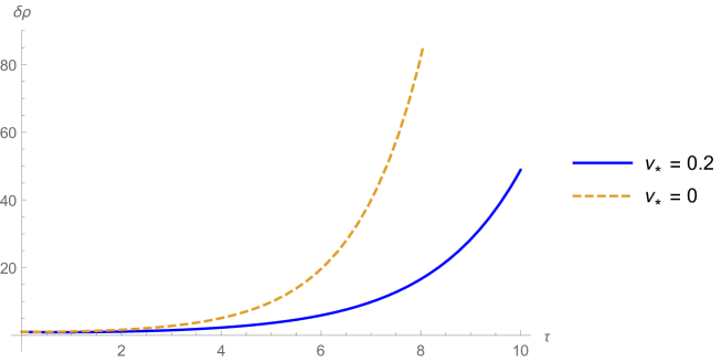
Figure 1: Density contrast $\delta\rho$ as function of the dimensionless time $\tau$ when $\lambda/\lambda_{J}=10$, for the dimensionless collision frequencies $\nu_{*}=0.1$ and $\nu_{*}=0$.

The differential equation (24) was solved numerically with the initial conditions $\delta\rho(10^{-3})=1$ and $\delta\rho^{\prime}(10^{-3})=0$. The solutions of the differential equation for the density contrast $\delta\rho$ as function of the dimensionless time $\tau$ are plotted in Figs. 1 and 2. The straight lines represent the case $\nu_{*}\neq 0$ where the collisions are taken into account while the dashed lines correspond to a collisionless Boltzmann equation where $\nu_{*}=0$.

In Fig. 1 the ratio between the Jeans wavelength $\lambda_{J}$ and the one associated with the perturbation $\lambda$ was chosen as $\lambda/\lambda_{J}=10$, the straight line corresponds to $\nu_{*}=0.2$ while the dashed line to $\nu_{*}=0$ (collisionless Boltzmann equation). In this case the perturbation wavelength is bigger than the Jeans wavelength and the density contrast grows with time which corresponds to Jeans instability. We note that due to the presence of the particle collisions an energy dissipation comes out implying a less accentuate growth of the density contrast in comparison to the one for a collisionless Boltzmann equation represented by $\nu_{*}=0$.

For the case where the perturbation wavelength is smaller than the Jeans wavelength, the density contrast has an oscillatory behavior in time. In Fig. 2 it is shown the time evolution of the density contrast for $\lambda/\lambda_{J}=0.1$, the straight line corresponding to $\nu_{*}=0.5$ and the dashed one to $\nu_{*}=0$. We note that the oscillatory behavior of density contrast is damped for the case where the particle collisions are taken into account due to the energy dissipation and in this case the density contrast fades away for big times.

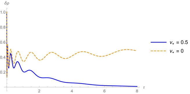
Figure 2: Density contrast $\delta\rho$ as function of the dimensionless time $\tau$ when $\lambda/\lambda_{J}=0.1$, for the dimensionless collision frequencies $\nu_{*}=0.1$ and $\nu_{*}=0$.

IV Conclusions

In this work the Jeans instability in an expanding Universe ruled by a spatially flat FLRW metric was analyzed within the framework of the BGK model of Boltzmann equation – where the collisions of the particles were taken into account – and Newtonian Poisson equation. The background distribution function – characterized by a comoving Maxwellian distribution – satisfies identically the BGK model of the Boltzmann equation. There is no necessity to invoke ”Jeans swindle”, since the background Newtonian gravitational potential satisfies the Poisson equation. The one-particle distribution function and the Newtonian gravitational potential were perturbed from their background states represented by plane waves of small amplitudes. The perturbed amplitude of the distribution function was considered as a function of the summational invariants. From the system of differential equations for the amplitudes a differential equation for the density contrast was obtained. This differential equation was solved numerically and it was shown that: (i) for perturbation wavelengths larger than Jeans wavelength the density contrast grows with time which characterizes Jeans instability. The growth of the density contrast is less accentuated for the case where the particle collisions are considered due to an energy dissipation; (ii) for perturbation wavelengths smaller than Jeans wavelength the density contrast has an oscillatory behavior in time. The oscillations for the case where the collisions are taken into account fade away in time due to the energy dissipation.

- [1] J. H. Jeans, Philos. Trans. R. Soc. A 199, 1 (1902)
- [2] S. Weinberg, Gravitation and cosmology. Principles and applications of the theory of relativity (Wiley, New York, 1972).
- [3] P. Coles and F. Lucchin, Cosmology. The Origin and Evolution of Cosmic structures, 2nd, edn. ( John Wiley, Chichester, 2002).
- [4] J. Binney and S. Tremaine Galactic Dynamics, 2nd. edn. (Princeton University Press, Princeton, 2008).
- [5] W. B. Bonnor, Mon. Not. R. Astr. Soc. 117, 104 (1957).
- [6] S. Capozziello, M. De Laurentis, I. De Martino, M. Formisano and S. D. Odintsov, Phys. Rev. D 85, 044022 (2012)
- [7] S. Capozziello and M. De Laurentis, Ann. Phys. 524, 545 (2012)
- [8] G. M. Kremer and R. André, Int. J. Mod. Phys. D 25, 1650012 (2016)
- [9] G. M. Kremer, AIP Conference Proceedings 1786, 160002 (2016)
- [10] I. De Martino and A. Capolupo, Eur. Phys. J. C 77, 715 (2017)
- [11] G. M. Kremer, M. G. Richarte and E. M. Schiefer, Eur. Phys. J. C 79, 492 (2019)
- [12] G. M. Kremer, Physica A 545, 123667 (2020)
- [13] S. A. Trigger, A. I. Ershkovich, G. J. F. van Heijst and P. P. J. M. Schram, Phys. Rev. E 69, 066403 (2004)
- [14] G. M. Kremer, M. G. Richarte and F. Teston, Phys. Rev. D 97, 023515 (2018).
- [15] G. M. Kremer, An introduction to the Boltzmann equation and transport processes in gases (Springer, Berlin, 2010).