Exact enumeration of satisfiable 2-SAT formulae

Abstract

We obtain exact expressions counting the satisfiable 2-SAT formulae and describe the structure of associated implication digraphs. Our approach is based on generating function manipulations. To reflect the combinatorial specificities of the implication digraphs, we introduce a new kind of generating function, the Implication generating function, inspired by the Graphic generating function used in digraph enumeration. Using the underlying recurrences, we make accurate numerical predictions of the phase transition curve of the 2-SAT problem inside the critical window. We expect these exact formulae to be amenable to rigorous asymptotic analysis using complex analytic tools, leading to a more detailed picture of the 2-SAT phase transition in the future.

1 Introduction

A $k$-CNF (Conjunctive Normal Form), or $k$-SAT formula, is a collection (conjunction) of clauses, where each clause is a disjunction of Boolean literals, and each Boolean literal is either a Boolean variable $x$ or its negation $\overline{x}$ (e.g. $(x_{1}\lor x_{2}\lor\overline{x}_{3})\land(\overline{x}_{1}\lor x_{3}\lor x_{4})$ for a $3$-CNF). A $k$-CNF is satisfiable if it returns $\mathrm{True}$ for at least one instantiation of its variables. More formal definitions are postponed until section 2.1.

The problem $k$-SAT of deciding whether a $k$-CNF is satisfiable is a central Constraint Satisfaction Problem (CSP for short). It is NP-complete for $k\geqslant 3$ [13], but $2$-SAT is solvable in polynomial [40, 26]. and even in linear [3] time. This linear algorithm for 2-SAT solving relies on the so-called implication digraphs which are digraphs built from the 2-CNF where each of the clauses $(x\lor y)$ is replaced with two directed edges $\overline{x}\to y$ and $\overline{y}\to x$, which corresponds to a logically equivalent replacement of disjunction by an implication (see further discussion in section 2.2). Although $2$-SAT is simple from a computational perspective, some of its variants are difficult. For example, the problem of counting the number of solutions of a $2$-SAT formula is NP-complete [29], and even approximating it within a factor less than $4/3$ is NP-complete [35].

The main contribution of the current paper is an exact expression for the number of satisfiable $2$-CNF with a given number of variables and clauses (other results are summarized in section 1.4). Our enumeration is expressed using generating functions and our tools are influenced by directed graph (digraph for short) enumeration. Before stating our results on the enumeration of satisfiable $2$-CNF in section 1.4, the three next subsections provide some historical background and discuss various angles of attack for the problem.

1.1 Exact enumeration

Graphs.

Graphical enumeration (see Harary and Palmer [34]) is a classical theme in enumerative combinatorics. It started in the late 19th century, with the enumeration of labeled trees by Borchardt [8] and Cayley [9]. Around a hundred years later, in a series of important papers, Wright [53, 54, 55] obtained exact expressions for the number of connected graphs according to their number of vertices and edges. Those expressions rely on the framework of generating functions, and excellent introductions to those tools are provided by Bergeron, Labelle, and Leroux [5], and Flajolet and Sedgewick [28].

Digraphs.

In the 1970’s, Liskovets, Robinson and Wright [52, 41, 48] developed the enumeration of strongly connected digraphs, directed acyclic graphs, and related digraph families. Most importantly, Robinson was able to lift the enumeration from the level of recurrences to the level of generating functions and obtain the tools to handle very general digraph families. Later, Robinson and Liskovets extended these methods to unlabeled enumeration. A detailed historical account on the development of the directed enumeration can be found in the introduction of [19], where this method has been again rediscovered.

2-CSP.

A CSP formula is similar to a CNF formula, but more logical operators are allowed, such as the XOR operation $\oplus$ and logical implication $\to$, further expanding to Boolean functions of more than two variables.

As various communities, namely computer scientists, probabilists and physicists [1, 7, 44], have been interested in CSP, in what follows we propose to present the line of research and the links between them that led us to approach the $2$-SAT problem via enumerative combinatorics and the use of generating functions. In a CSP formula where each clause relates to exactly $2$ variables (or $2$-CSP), it is very natural to represent the whole formula, i.e. the collection of clauses, via a graph where the clauses (resp. the variables) are the edges (resp. the nodes) of the graph.

As far as graphs are concerned, the works of Daudé and Ravelomanana [15] and Pittel and Yeum [46] show that analyses based on graphical enumeration [53, 55, 34] play a substantial role as such an approach lead to remarkably accurate results on the probability of satisfaction of a random formula. In the aforementioned works, the enumerative approach consists in encoding the objects to be enumerated with the help of generating functions. Over the past decade (see [15, 19, 47, 24] for reference) it has turned out that it is fundamental to understand how to enumerate directed graphs before tackling the enumeration of $2$-SAT formulae.

1.2 Structure and phase transition

Graphs.

The two most natural models of random graphs are $G(n,m)$ and $G(n,p)$. Both generate graphs on $n$ vertices. $G(n,m)$ also fixes the number $m$ of edges and samples the graph uniformly at random, while $G(n,p)$ adds an edge between each pair of vertices independently with probability $p$. Random graphs with a large number of vertices exhibit similar limit statistical properties in both models, as shown by Bollobás [6].

Erdős and Rényi [25] studied the structure of random $G(n,m)$ graphs. Let us transpose in the $G(n,p)$ model one of their most striking results. For $p=c/n$, with probability tending to $1$, a random $G(n,p)$ graph contains, as $n\to\infty$,

• only trees and unicycles (components having only one cycle) if $c<1$,

• only trees, unicycles, and a unique “giant” component, of size $n\cdot f(c)+o(n)$, if $c>1$.

Such a drastic change of behavior is called a phase transition (a term borrowed from theoretical physics). The typical structure of random $G(n,p)$ graphs for $p$ close to $1/n$ was investigated by Stepanov [50] and described in fine detail by Janson, Knuth, Łuczak and Pittel [36]. They showed that in the critical window, corresponding to $p=\frac{1}{n}(1+O(n^{-1/3}))$, a random $G(n,p)$ graph has a positive limit probability to contain several connected components that are neither trees nor unicycles. They also derived the limit distributions for various statistics of those components. As we discuss below, the satisfiability of random $2$-SAT formulae undergoes a similar phase transition. Finally, an even more precise description of large graphs in the critical window has been obtained by Addario-Berry, Broutin and Goldschmidt [2], in the form of a scaling limit (a geometrical limit for random graphs with a large number of vertices expressed in terms of various stochastic processes related to the Brownian motion).

Digraphs.

The random models $G(n,m)$ and $G(n,p)$ extend naturally to digraphs. In the $D(n,p)$ model, the generated digraph has $n$ vertices and each of the $n(n-1)$ ordered pairs of distinct vertices becomes an arc independently with probability $p$. As in the case of graph, the structure of digraphs undergoes a phase transition, located by Karp [38] and Łuczak [42]. With probability tending to $1$ as $n$ tends to infinity, the strongly connected components of a random $D(n,c/n)$ digraph are

• cycles or single vertices if $c<1$,

• cycles, single vertices, and a unique giant strong component containing a linear proportion of all vertices if $c>1$.

Łuczak and Seierstad [43] derived the width $n^{-1/3}$ of the critical window. For $p=\frac{1}{n}(1+O(n^{-1/3}))$, they established that the size of the largest strongly connected component is of order $n^{1/3}$. Recently, Goldschmidt and Stephenson [32] derived a scaling limit for random digraphs inside the critical window. Using a generating function approach, Dovgal, de Panafieu, Ralaivaosaona, Rasendrahasina and Wagner [24] also obtained precise information on the typical structure of random $D(n,p)$ digraphs inside the critical window.

2-SAT.

In the scope of the current paper, we assume that inside of all the clauses of a 2-CNF, the literals have distinct Boolean variables. This results in $2n(n-1)$ possible clauses in case of $n$ variables. As for graphs, there are two natural models for random 2-CNF. In the $(n,m)$ model, the numbers of variables $n$ and clauses $m$ are fixed, and the formula is sampled uniformly at random. This is akin to the $G(n,m)$ random graph model. In the $(n,p)$ model, the number of variables $n$ and a probability $p$ are fixed, and the formula is built by adding each of the $2n(n-1)$ possible clauses independently with probability $p$. This second model is akin to the $G(n,p)$ random graph model. As in the case of graphs, we expect random formulae to behave similarly under both models as $n$ tends to infinity. We refer to [7] for details regarding the correspondence between these models as $n\to\infty$.

Our enumerative results allow us to express exactly the probability for a random formula to be satisfiable in the $(n,m)$ model. In proposition 3.3, we show how to translate this result to the $(n,p)$ model as well. The most popular model for random 2-SAT formulae is the $(n,p)$ model, so we focus on it in the rest of the discussion.

Let $\mathbb{P}_{\mathrm{SAT}}(n,p)$ denote the probability for a random $(n,p)$ CNF to be satisfiable. It was shown by Goerdt [31], Chvátal and Reed [10] and Fernandez de la Vega [16] that the limit of $\mathbb{P}_{\mathrm{SAT}}(n,p)$ is $1$ for $p=c/n$ with $c<1/2$, and $0$ if $c>1/2$. This sharp change is called the phase transition of $2$-SAT. Bollobás, Borgs, Chayes, Kim and Wilson [7] refined their predictions and showed that the limit probability of satisfiability $\mathbb{P}_{\mathrm{SAT}}(n,p)$ is $1-\Theta(|\mu|^{-3})$ (or, respectively, $\exp(-\Theta(\mu^{3}))$) for $p=\frac{1}{2n}\left(1+\mu n^{-1/3}\right)$ when $\mu\to-\infty$ (or, respectively, $\mu\to+\infty$), suggesting that the only region where this probability could be non-trivial is for $\mu$ staying in a compact real interval. Some of these estimated were further refined by Kim [39] through Poisson cloning and Dovgal [23] with a different technique. Further results on MAX SAT around the phase transition window have been obtained in [14].

To describe the behavior of this phase transition, we say that the critical window has width $n^{-1/3}$. Let use define $\mathbb{P}_{\mathrm{SAT},\infty}(\mu)$ as the limit

$$\mathbb{P}_{\mathrm{SAT},\infty}(\mu)=\lim_{n\to+\infty}\mathbb{P}_{\mathrm{SAT}}\left(n,\frac{1}{2n}\left(1+\mu n^{-1/3}\right)\right).$$

A question of interest in the study of phase transitions is the computation of the function $\mathbb{P}_{\mathrm{SAT},\infty}(\mu)$. In the current paper, we obtain exact expressions for the number of satisfiable 2-CNF that are related to, though more complex than, the expressions counting digraph families. Our hope is that the analytic tools developed by [24] to analyze the phase transition of digraphs can be extended to 2-CNF and express $\mathbb{P}_{\mathrm{SAT},\infty}(\mu)$. We also use those exact expressions to obtain highly accurate (although non-rigorous) numerical predictions of the curve of $\mathbb{P}_{\mathrm{SAT},\infty}(\mu)$.

1.3 Discussion of possible strategies

In the current work, we focus on the exact enumeration of families related to $2$-SAT formulae. To do this, we further extend the symbolic method for enumeration of directed graphs. Indeed, digraphs are closely related to $2$-SAT formulae since the latter can be represented using implication digraphs. An unsatisfiable formula is distinguished by the presence of a specific subgraph – a contradictory circuit – inside its implication digraph. We refer to an approach of Collet, de Panafieu, Gardy, Gittenberger and Ravelomanana [12] based on finding induced subgraphs in random graphs, using generating functions as well. Unfortunately, such an approach does not allow to capture the counting recurrence in an efficient way, because the family of the required patterns is too large.

Another possible approach is an inclusion-exclusion method, or a more refined probabilistic tool based on distinguishing a random variable inside a formula, i.e. statistic. Two particular statistics can be used to count 2-SAT formulae: the number of Boolean assignments satisfying the formula, and the number of contradictory variables (defined below). A 2-SAT formula is satisfiable if and only if it has at least one satisfiable assignment. Equivalently, it is satisfiable if and only if it contains no contradictory variable. Other statistics have historically been used to produce upper and lower bounds on the probability that a random formula is satisfiable.

The expression obtained by applying inclusion-exclusion on the number of satisfiable Boolean assignments indeed gives a computable expression, which, however, produces an exponential number of summands. This approach is not promising, neither from a computational nor from a theoretical viewpoint, due to the rapid growth of magnitude of the alternating terms. On the other hand, the first moment method applied to the number of satisfiable Boolean assignments provides bounds on the location of the phase transition, while the second moment method requires a more delicate choice of the underlying random variable and fails to provide a tight bound with this statistic for general $k$-SAT. Recent breakthroughs in the asymptotic threshold of $k$-SAT for large $k$ [22, 11] also rely on a careful choice of the right statistic: the authors consider clusters of solutions instead of the total number of satisfying assignments.

Let us briefly turn to the work of Bollobás, Borgs, Chayes, Kim and Wilson [7]. Let us write $H\subset F$ if the clauses of the CNF $H$ are included in the clauses of the CNF $F$. In the combinatorial study of random 2-SAT, and more generally, $k$-SAT, one of the key features of a random formula has been its spine, which is defined as

$$S(F)=\{x\,|\,\exists H\subset F,\,H\text{ is }\mathrm{SAT}\text{ and }H\land x\text{ is }\mathrm{UNSAT}\}\,.$$

The spine can be seen as a set of literals that are forced to take False values in any satisfying assignment. However, for unsatisfiable formulae the spine is also well-defined. As an alternative to this purely logical definition, a spine in the implication digraph can be defined as the set of literals $x$ for which there exists a directed path from $x$ to $\overline{x}$. In other terms, the spine of a formula $F$ is defined as the set of literals $x$ such that there exists a satisfiable subformula $H$ of $F$ with the property that $H$ is SAT but $H\land x$ is not satisfiable. Consequently, when building a formula by adding random clauses one after the other starting from the empty formula, the spine has proven to be a useful concept for calculating the probability of satisfiability of the formula. Introducing this concept allowed the authors of [7] to establish the width $n^{-1/3}$ of the critical window of the phase transition in 2-SAT, i.e. to prove that the limit of the probability $\mathbb{P}_{\mathrm{SAT}}(n,p)$ could only be non-trivial for $p=\frac{1}{2n}(1+O(n^{-1/3}))$.

In the current paper, we are considering the so-called contradictory strongly connected components as the central parameter. In an implication digraph, a variable $x$ is contradictory if there is a path from $x$ to $\overline{x}$ and from $\overline{x}$ to $x$, and the whole strongly connected component containing a contradictory variable is called contradictory (we will show that, in fact, every variable of this component will also be contradictory). On the level of logical definition, a Boolean variable $x$ is called contradictory if both its literals $x$ and $\overline{x}$ belong to the spine. Equivalently, the set of contradictory variables is defined as

$$C(F)=\{x\,|\,\exists H_{1},H_{2}\subset F,\,H_{1},H_{2}\text{ are $\mathrm{SAT}$ and }H_{1}\land x\text{ and }H_{2}\land\overline{x}\text{ are $\mathrm{UNSAT}$}\}.$$

This definition can be possibly extended to CSP models other than 2-SAT.

1.4 Our results

Exact enumeration.

In the current paper, we express the number of satisfiable 2-CNF formulae with the help of generating functions. It follows from proposition 4.5 that if $a_{n,m}$ denotes the number of satisfiable 2-CNF with $n$ Boolean variables and $m$ clauses, then $a_{n,m}$ can be encoded into a generating function identified by the expression

$$\sum_{n\geqslant 0}\dfrac{1}{(1+w)^{n(n-1)}}\dfrac{z^{n}}{2^{n}n!}\sum_{m\geqslant 0}a_{n,m}w^{m}=\dfrac{\displaystyle\sum\limits_{n\geqslant 0}\frac{1}{(1+w)^{n(n-1)}}\frac{z^{n}}{2^{n}n!}\odot_{z}e^{-\mathrm{SCC}(2z,w)/2}}{\displaystyle\sum\limits_{n\geqslant 0}\frac{1}{(1+w)^{{n\choose 2}}}\frac{z^{n}}{n!}\odot_{z}e^{-\mathrm{SCC}(z,w)}}\,,$$

where $\odot_{z}$ denotes the exponential Hadamard product

$$\sum_{n\geqslant 0}a_{n}(w)\dfrac{z^{n}}{n!}\odot_{z}\sum_{n\geqslant 0}b_{n}(w)\dfrac{z^{n}}{n!}:=\sum_{n\geqslant 0}a_{n}(w)b_{n}(w)\dfrac{z^{n}}{n!}\,,$$

and $\mathrm{SCC}(z,w)$ is the Exponential generating function of strongly connected digraphs (see  [19, Corollary 3.5] or eq. 2 below). Note that negative signs in formal generating functions can often be interpreted as an application of the inclusion-exclusion principle, as explained by [33, Lemma 2.2.29] (see also [28, III. 7.4, p. 206]). In our case, the inclusion-exclusion manifests itself in the negative exponential terms, and the corresponding statistical patterns inside a random implication digraph are the number of the so-called contradictory and ordinary strongly connected components.

We obtain two exact expressions for the number of satisfiable 2-SAT formulae (theorem 4.6 and theorem 4.7), the number of unsatisfiable 2-SAT formulae whose implication digraph is strongly connected (theorem 4.8) as well as a description of the structure of the implication digraphs associated to 2-SAT formulae (theorem 4.9): the latter result describes the implication digraphs with given allowed strongly connected components. Those results are based on generating function manipulations. In this paper, we introduce a new type of generating function, called an Implication generating function. It is inspired by the Special or Graphic generating function introduced in [48, 30]. The product of an Implication generating function with a Graphic generating function corresponds to a combinatorial operation involving a digraph and a 2-SAT formula, that we call hereafter an implication product.

Phase transition.

Note that Deroulers and Monasson [21] gave numerical estimates of probabilities of these formula being satisfiable around their phase transition. Up to $n=5\times 10^{6}$, they were able to determine the empirical values of

$$\mathbb{P}\left[\mbox{Random $2$-SAT formula built with $n$ variables and $n$ clauses is SAT}\right]$$

using Monte-Carlo simulation, and gave a prediction of $\mathbb{P}_{\mathrm{SAT},\infty}(0)=0.907\pm 10^{-3}.$ Our results translate into more efficient algorithms to accurately but non-rigorously predict those empirical values. We improve their prediction to $\mathbb{P}_{\mathrm{SAT},\infty}(0)=0.90622396067\pm 10^{-11},$ and also make prediction for $\mathbb{P}_{\mathrm{SAT},\infty}(\mu)$ for other values of $\mu$, plotting the phase transition curve of the 2-SAT inside the critical window, viz. fig. 1. For the sake of reproducibility, we share the ipython notebooks used for computation of these values by a hopefully permanent public URL on GitLab

https://gitlab.com/sergey-dovgal/enumeration-2sat-aux

Other researchers are encouraged to reuse them if they wish so. Given the similarity between the exact expressions counting digraph families and satisfiable 2-CNF, we hope that the analytic tools for analysis of the phase transition of digraphs similar to the ones developed by [24] can be extended to 2-CNF and express $\mathbb{P}_{\mathrm{SAT},\infty}(\mu)$ in a closed form. We expect this curve to have an expression akin to the integrals of Airy functions such as those encountered in [24], or some form of generalized Airy function (see [36, 17]).

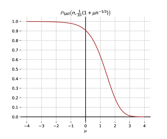
Figure 1: The predicted limiting probability that a formula is satisfiable inside the critical window of the 2-SAT phase transition, in the model $(n,p)$, where $n$ denotes the number of Boolean variables, and $p$ is the clause probability, $p=\frac{1}{2n}(1+\mu n^{-1/3})$.

Outline of the paper

We recall the classic definitions of 2-SAT formulae as well as the characterization of satisfiable formulae and the structure of the associated implication digraphs in section 2. The various types of generating functions used throughout this article are introduced in section 3. Then, section 4 presents our results and their proofs. Finally, in section 5 we provide the first several terms of the counting sequences for some 2-SAT families along with accurate numerical predictions related to the satisfiability phase transition.

2 Conjunctive Normal Forms and implication digraphs

2.1 Definitions and notation

In this section, we are using the classical binary Boolean operators $\lor,\land$ and $\to$ which correspond respectively to disjunction, conjunction and implication. We are also using the unary operator $\neg x$ or $\overline{x}$ to denote negation.

Definition 2.1.

The literals of a Boolean variable $x$ are $x$ and its negation $\overline{x}$. A Conjunctive Normal Form (CNF) formula on $n$ variables is a set (conjunction) of clauses, where each clause is a disjunction of literals corresponding to distinct variables.

For example, the formula (viz. fig. 3)

$$(x_{1}\vee x_{3})\land(\overline{x}_{2}\vee x_{1})\land(x_{2}\vee\overline{x}_{3})$$ (1)

is considered to be the same CNF as

$$(x_{1}\vee\overline{x}_{2})\land(x_{2}\vee\overline{x}_{3})\land(x_{3}\vee x_{1}).$$

Throughout this work, we do not consider formulae with literal or clause duplications, such as

$$(x_{1}\vee\overline{x}_{1}) \land(x_{2}\vee x_{1}),$$

$$(x_{1}\vee\overline{x}_{2}) \land(\overline{x}_{2}\vee x_{1}).$$

Definition 2.2.

A CNF is satisfiable if there exists an assignment of Boolean values to the variables that satisfies each clause. A 2-CNF (or 2-SAT formula) is a CNF where each clause contains exactly two (distinct) literals.

We also define a second type of Boolean formulae, as an intermediate step between $2$-CNF and directed graphs (digraphs).

Definition 2.3.

An implication formula on $n$ variables is a set of clauses, where each clause is the implication of two literals corresponding to distinct variables.

Figure 2: An example of a 2-CNF depicted in a form of a labeled graph with decorations. Literals $x_{k}$ and $\overline{x}_{k}$ are replaced with $k$ and $\overline{k}$ for brevity.

Figure 3: The corresponding implication digraph. Literals $x_{k}$ and $\overline{x}_{k}$ are replaced with $k$ and $\overline{k}$ for brevity.

Since the clause $x\vee y$ is equivalent with either of the clauses $(\overline{x}\to y)$, $(\overline{y}\to x)$, and with their conjunction $(\overline{x}\to y)\land(\overline{y}\to x)$, any 2-CNF has an equivalent implication formula. Reciprocally, any implication formula where each clause $x\to y$ has its symmetric $\overline{y}\to\overline{x}$ also corresponds to a valid 2-CNF. For example (viz. fig. 3), the implication formula corresponding to (1) is

$$(\overline{x}_{1}\to x_{3})\land(\overline{x}_{3}\to x_{1})\land(x_{2}\to x_{1})\land(\overline{x}_{1}\to\overline{x}_{2})\land(\overline{x}_{2}\to\overline{x}_{3})\land(x_{3}\to x_{2}).$$

Therefore, a 2-CNF is satisfiable if and only if the corresponding implication formula is satisfiable.

To each 2-CNF on $n$ variables with $m$ clauses, there corresponds an implication digraph with $2n$ vertices and $2m$ arcs: each clause $(k,\ell)$ corresponds to the arcs $(\overline{k},\ell)$ and $(\overline{\ell},k)$. Since a clause cannot contain twice the same variable, an implication digraph contains neither loops nor arcs from a literal to its negation. Since a 2-CNF does not contain twice the same clause, there is at most one arc between any two literals.

Definition 2.4.

A contradictory variable in a 2-CNF is a variable $x$ such that the implication digraph contains oriented paths from $x$ to $\overline{x}$ and from $\overline{x}$ to $x$. A strongly connected component (SCC) of a digraph is a set of vertices, maximal for the inclusion with respect to the property that an oriented path exists between any two vertices from the set. In an implication digraph, a contradictory strongly connected component (contradictory SCC) is an SCC that contains a contradictory variable. An SCC that is not contradictory is ordinary.

Definition 2.5.

An SCC of a digraph is source-like if there is no arc pointing to any of its vertices from a vertex outside of it. It is sink-like if there is no arc pointing from any of its vertices to a vertex outside of it. It is isolated if it is both source-like and sink-like.

Definition 2.6.

Consider a digraph $D$ whose vertices form a subset of literals $\{x_{1},\ldots,x_{n},\overline{x}_{1},\ldots,\overline{x}_{n}\}$. The negation $\overline{D}$ of $D$ is formed by replacing its vertex labels with their negations and flipping the edge directions: if the original digraph $D$ contains an arc $x\to y$, then its negated digraph contains an arc $\overline{y}\to\overline{x}$ instead.

Figure 4: A condensation of 2-CNF implication digraph. Each component is depicted as a node. An arrow from component $D$ to component $E$ means that there is at least one edge $u\rightarrow v$ in the implication digraph with the literal $u$ in $D$ and the literal $v$ in $E$.

Figure 5: An ordinary component.

Figure 6: A contradictory component.

In fig. 6 we provide an example, where an implication digraph of a 2-CNF formula is depicted in a condensated form, the components $X=\overline{X}$ and $Y=\overline{Y}$ are contradictory SCCs; $A$, $\overline{B}$, $C$ and $\overline{C}$ are ordinary source-like SCCs; $\overline{A}$, $B$, $C$ and $\overline{C}$ are ordinary sink-like SCCs; and finally, $C$ and $\overline{C}$ are ordinary isolated SCCs. Figures 6 and 6 provide examples of an ordinary and a contradictory component.

2.2 Structural properties of 2-Conjunctive Normal Forms

The first linear time algorithm to decide the satisfiability of a 2-SAT formula was designed by Aspvall, Plass and Tarjan [3]. It relied on a characterization of the implication digraphs of satisfiable 2-SAT formulae. In this section, we recall their proof, reformulating it to fit our needs.

We start with properties of the contradictory SCCs of implication digraphs.

Proposition 2.7.

Let $C$ be a contradictory SCC. Then,

1. All variables appearing in $C$ are contradictory;

2. If $C$ is source-like (or sink-like) then it is isolated;

3. If $C^{\prime}$ is another contradictory SCC, then there is no oriented path starting in $C$ and ending in $C^{\prime}$.

Proof.

If $C$ is reduced to one variable, the assertion is trivial. So, let $C$ be a contradictory SCC that contains a contradictory variable $x$ and a literal $k$. Then $C$ contains oriented paths from $x$ to $\overline{x}$, from $\overline{x}$ to $x$, from $x$ to $k$ and from $k$ to $x$. By symmetry of the arcs, this implies the existence of oriented paths from $\overline{k}$ to $\overline{x}$ and $\overline{x}$ to $\overline{k}$. Combining them, we obtain oriented paths from $k$ to $\overline{k}$ and $\overline{k}$ to $k$. Thus, $k$ is also a contradictory variable.

For the second part, suppose that $C$ is source-like. If there were an arc from a literal $k\in C$ to a literal $\ell$ outside of $C$, then by symmetry we would also have the arc $(\overline{\ell},\overline{k})$. By the previous result, $\overline{\ell}$ does not belong to $C$, but $\overline{k}$ does. Thus, $C$ would not be source-like, which leads to a contradiction.

Let us prove the last part of the proposition. By symmetry, an oriented path from a literal $k$ of the contradictory SCC $C$ to a literal $\ell$ of the contradictory SCC $C^{\prime}$ implies an oriented path from $\overline{\ell}$ to $\overline{k}$, hence from $C^{\prime}$ to $C$. Thus, $C$ and $C^{\prime}$ are the same contradictory SCC. ∎

We now turn to ordinary source-like SCC.

Proposition 2.8.

Let $C$ denote a source-like (resp. sink-like, resp. isolated) ordinary SCC from the implication digraph, then the component $\overline{C}$ is a sink-like (resp. source-like, resp. isolated) SCC which is disjoint from $C$.

Proof.

It is sufficient to prove that if $C$ is ordinary and source-like, then $\overline{C}$ is a sink-like SCC. Since each arc $(k,\ell)$ has its symmetric $(\overline{\ell},\overline{k})$, any oriented path from $k$ to $\ell$ has as symmetric an oriented path from $\overline{\ell}$ to $\overline{k}$. Thus, the negation of the literals from $C$ also form an SCC $\overline{C}$. It is disjoint from $C$ because $C$ is not contradictory. Furthermore, any arc pointing from $\overline{C}$ to a literal $k$ outside $\overline{C}$ would have its symmetric pointing to $C$ from $\overline{k}$. The literal $\overline{k}$ could not belong to $C$, otherwise $k$ would be in $\overline{C}$. Thus, $C$ would not be source-like: a contradiction. It follows that such a $k$ cannot exist and that $\overline{C}$ is sink-like. ∎

We finally arrive at the classic characterization of satisfiable 2-CNF.

Proposition 2.9.

A 2-CNF is satisfiable if and only if it contains no contradictory variable.

Proof.

Given an implication digraph, let us write $x\rightsquigarrow y$ if there exists an oriented path from the literal $x$ to the literal $y$. Suppose that a formula contains a contradictory variable and is satisfiable, which means that all variables can be assigned Boolean values satisfying all the clauses. If $x$ is a contradictory variable, then in the implication digraph, the presence of an oriented path $x\rightsquigarrow\overline{x}$ results in the logical implication $x\Rightarrow\overline{x}$, so $x$ must take the value $\mathrm{False}$. Similarly, the oriented path $\overline{x}\rightsquigarrow x$ implies $\overline{x}\Rightarrow x$, so $x$ must be $\mathrm{True}$. This is a contradiction, so the formula cannot be satisfiable if it contains a contradictory variable.

We prove the reverse by induction on the number of variables. Consider a 2-CNF without contradictory variables, and assume that any smaller 2-CNF without contradictory variables is satisfiable. Then, it must contain a source-like SCC. Let $C$ be any source-like SCC of the implication digraph. By proposition 2.8, its symmetric $\overline{C}$ is sink-like. Let us set all the literals of $C$ to the Boolean value $\mathrm{False}$, so the literals from $\overline{C}$ are set to $\mathrm{True}$. Consider the formula $F$ corresponding to removing the variables from $C$ and $\overline{C}$. It contains no contradictory variable, so it is satisfiable by induction. We claim that any solution to $F$ satisfies the original formula. Indeed, the arcs we removed are from $C$, in which case they become $\mathrm{False}\Rightarrow x$ which is satisfied for any value of $x$, or to $\overline{C}$, in which case they become $x\Rightarrow\mathrm{True}$ which is satisfied for any value of $x$. ∎

3 Generating functions and implication product

This section introduces the tools that will be applied in section 4 for counting various $2$-SAT families. First, let us recall the general definition of generating functions and give a brief overview of the plan of the section.

A generating function (GF) associated to a family $\mathcal{A}$ is a formal series of the form

$$A(z)=\sum_{a\in\mathcal{A}}\kappa_{|a|}(z),$$

where $z$ is a formal variable, $|a|$ is a non-negative integer number computed from $a$ and called the size of $a$, and $(\kappa_{n}(z))_{n\geqslant 0}$ is a sequence of functions. Let $a_{n}$ denote the number of elements $a\in\mathcal{A}$ such that $|a|=n$, and assume $a_{n}$ is finite for all $n\geqslant 0$. Grouping the summands corresponding to the same value $|a|$, the GF becomes

$$A(z)=\sum_{n\geqslant 0}a_{n}\kappa_{n}(z).$$

The type of the GF corresponds to the choice of $(\kappa_{n}(z))$. The founding idea of analytic number theory [51], species theory [5] and analytic combinatorics [28] is that the study of the sequence $(a_{n})$ can be simplified by the introduction of the right type of GF.

In this article, we will use several types of GFs, defined in section 3.1

• the classic Ordinary and Exponential GFs correspond to

  $$\kappa_{n}(z)=z^{n}\qquad\text{and}\qquad\kappa_{n}(z)=z^{n}/n!,$$

  and a good reference is [28, Chapters I and II],

• Graphic (or Special) GFs, introduced by Robinson [48] and Gessel [30], correspond to

  $$\kappa_{n}(z)=\frac{1}{(1+w)^{\binom{n}{2}}}\frac{z^{n}}{n!}$$

  where $w$ denotes an additional formal variable,

• and a new type of GFs, which we call Implication GFs, that corresponds to

  $$\kappa_{n}(z)=\frac{1}{(1+w)^{n(n-1)}}\frac{z^{n}}{2^{n}n!}\,.$$

The Implication GF is designed for the enumeration of various $2$-CNF families. To translate GFs of a type into another type, we will use the exponential Hadamard product, introduced by Joyal (see remark 3.4). It is presented in section 3.2. The central idea behind the use of GFs is that combinatorial operations on the families translate into analytic operations on their GFs. The type of GF used depends on the combinatorial operation of interest. section 3.3 presents those operations for the various types used in this paper.

3.1 Types of generating functions

We present the various types of GFs used in this paper in the specific context of graphs, digraphs and implication digraphs. General introductions to Ordinary and Exponential GFs are available in [5] and [28]. The definition of Graphic (or Special) GFs is due to Robinson [48] and Gessel [30]. The definition of Implication GFs is new and will be motivated in section 3.3. In this paper we are dealing with labeled objects: for each graph or digraph with $n$ vertices, we consider that their vertices are labeled with distinct labels from $\{1,\ldots,n\}$ (more on that also in section 3.3).

Definition 3.1.

Let $\mathcal{A}$ be a graph or digraph family and $\mathcal{B}$ an implication digraph family. Let $a_{n,m}$ denote the number of (di)graphs in $\mathcal{A}$ with $n$ vertices and $m$ arcs (resp. edges), and $b_{n,m}$ the number of implication digraphs in $\mathcal{B}$ with $2n$ vertices and $2m$ implication arcs (i.e. built from 2-CNFs with $n$ variables and $m$ clauses). For each $n$, let $\mathcal{A}_{n}$ denote the subfamily of $\mathcal{A}$ of (di)graphs on $n$ vertices, and $\mathcal{B}_{n}$ the subfamily of $\mathcal{B}$ of implication digraphs on $2n$ vertices.

The Ordinary GFs of $\mathcal{A}_{n}$ and $\mathcal{B}_{n}$ are defined as

$$a_{n}(w)=\sum_{m\geqslant 0}a_{n,m}w^{m}\qquad\text{and}\qquad b_{n}(w)=\sum_{m\geqslant 0}b_{n,m}w^{m}.$$

The Exponential GF $A(z,w)$, Graphic GF $\widehat{A}(z,w)$ and Implication GF $\ddot{B}(z,w)$ are defined as

$$A(z,w)=\sum_{n\geqslant 0}a_{n}(w)\frac{z^{n}}{n!},\quad\widehat{A}(z,w)=\sum_{n\geqslant 0}\frac{a_{n}(w)}{(1+w)^{\binom{n}{2}}}\frac{z^{n}}{n!}\quad\text{and}\quad\ddot{B}(z,w)=\sum_{n\geqslant 0}\frac{b_{n}(w)}{(1+w)^{n(n-1)}}\frac{z^{n}}{2^{n}n!}.$$

To alleviate the notations, we often omit the variable $w$, writing $A(z)$ instead of $A(z,w)$. As a convention, we will use hats to distinguish Graphic GFs from Exponential GFs, and double dots to denote Implication GFs.

The name Graphic of the generating function may be somewhat misleading: we always use Exponential GFs to enumerate graphs, and often use Graphic GFs to enumerate directed graphs. However, for historical reasons, we are keeping its original name.

The following lemma expresses the generating functions of various families that will be used throughout this article.

Lemma 3.2.

Let $G(z)$ (variable $w$ omitted) denote the Exponential GF of all graphs with labeled vertices, where loops and multiple edges are forbidden, then

$$G(z)=\sum_{n\geqslant 0}(1+w)^{\binom{n}{2}}\frac{z^{n}}{n!}.$$

Let $D(z)$ denote the Exponential GF of all digraphs, with labeled vertices, where loops and multiple arcs are forbidden. In this model, we assume that between any two nodes of a digraph, both arcs connecting these nodes can be present. Then

$$D(z)=\sum_{n\geqslant 0}(1+w)^{n(n-1)}\frac{z^{n}}{n!}.$$

Let $\widehat{\mathbf{Set}}(z)$ denote the Graphic GF of digraphs that contain no arcs, then

$$\widehat{\mathbf{Set}}(z)=\sum_{n\geqslant 0}\frac{1}{(1+w)^{\binom{n}{2}}}\frac{z^{n}}{n!}.$$

Let $\ddot{\mathbf{Set}}(z)$ denote the Implication GF of implication digraphs that contain no arcs, then

$$\ddot{\mathbf{Set}}(z)=\sum_{n\geqslant 0}\frac{1}{(1+w)^{n(n-1)}}\frac{z^{n}}{2^{n}n!}.$$

Proof.

Consider a family $\mathcal{A}$ of graphs (resp. digraphs, resp. implication digraphs) and let $a_{n,m}$ denote the number of its elements with $n$ vertices (resp. $n$ vertices, resp. $2n$ vertices) and $m$ edges (resp. $m$ arcs, resp. $2m$ arcs). Let $a_{n}(w)$ denote its Ordinary GF

$$a_{n}(w)=\sum_{m\geqslant 0}a_{n,m}w^{m}.$$

The number of graphs with $n$ vertices and $m$ edges is $\binom{\binom{n}{2}}{m}$, because a subset of $m$ edges is chosen among all possible $\binom{n}{2}$ edges. Thus, if $\mathcal{A}$ is the family of all graphs, then $a_{n}(w)=(1+w)^{\binom{n}{2}}$ and the first result follows. When $\mathcal{A}$ is the family of all digraphs, we have $a_{n,m}=\binom{n(n-1)}{m}$, because a subset of $m$ arcs is chosen among all possible $n(n-1)$ arcs. Thus, $a_{n}(w)=(1+w)^{n(n-1)}$, which implies the second result. When $\mathcal{A}$ is the family of digraphs without any arc, we have $a_{n}(w)=1$, because there exists only one digraph on $n$ vertices containing no arc. This implies the third result. Similarly, when $\mathcal{A}$ is the family of implication digraphs containing no arc, we have again $a_{n}(w)=1$. This implies the fourth result. ∎

We choose the notations $\widehat{\mathbf{Set}}$ and $\ddot{\mathbf{Set}}$ to represent families that are just set of vertices, without any additional structure. Note that in all the sums of the last lemma, $n=0$ corresponds to the empty graph, containing no vertices.

Probability from generating functions.

It is handy to use generating functions to calculate the probabilities in the $(n,p)$ model, where the number of clauses is not fixed, but each clause is drawn independently with probability $p$ (c.f. [47, Lemma 6] or [24, Lemma 2.8]).

Proposition 3.3.

Let $\mathcal{F}$ be some family of 2-SAT formulae, whose Implication GF is $\ddot{F}(z,w)$. Then, the probability that a random formula from the $(n,p)$ model (i.e. a random formula with $n$ Boolean variables where each of the $2n(n-1)$ possible clauses is drawn independently with probability $p$) belongs to $\mathcal{F}$, is

$$\mathbb{P}_{n,p}(F\in\mathcal{F})=2^{n}n!(1-p)^{n(n-1)}[z^{n}]\ddot{F}\left(z,\frac{p}{1-p}\right).$$

Proof.

Let $m(F)$ denote the number of clauses of a formula $F$, and let $\mathcal{F}_{n}$ be the set of the formulae from $\mathcal{F}$ containing $n$ Boolean variables. There are $2n(n-1)$ possible clauses for $n$ Boolean variables. The probability that a random formula $F$ belongs to $\mathcal{F}_{n}$ is expressed by summing over all possible numbers of edges

$$\mathbb{P}_{n,p}(F\in\mathcal{F}) =\sum_{F\in\mathcal{F}_{n}}p^{m(F)}(1-p)^{2n(n-1)-m(F)}$$

$$=(1-p)^{2n(n-1)}\sum_{F\in\mathcal{F}_{n}}\left(\dfrac{p}{1-p}\right)^{m(F)}$$

$$=(1-p)^{2n(n-1)}\left.(1+w)^{n(n-1)}\right|_{w=\frac{p}{1-p}}2^{n}n![z^{n}]\ddot{F}\left(z,\dfrac{p}{1-p}\right)$$

$$=2^{n}n!(1-p)^{n(n-1)}[z^{n}]\ddot{F}\left(z,\dfrac{p}{1-p}\right).$$

∎

Multivariate generating functions.

For graph-like families, we use GFs with two variables: $z$ marking the number of vertices and $w$ the number of edges. Additional marking variables can be introduced. There are two ways to define the generating function with several variables. One way is to consider generalized counting sequences (such as $a_{n,k,j}$ in the case of three parameters), and take the sum over all possible combination of indices (e.g. $A(z,w,u):=\sum_{n,k,j\geqslant 0}a_{n,k,j}u^{j}w^{k}\frac{z^{n}}{n!}$). Another viewpoint is to say that the objects inside the family do not have the same weight, and an object receives a weight $u^{j}$ if the corresponding parameter marked by the variable $u$ inside this object is equal to $j$. In this case we return to the usual counting sequence with one variable $\sum_{n\geqslant 0}a_{n}\frac{z^{n}}{n!}$, where $a_{n}$ now denotes the total weight of the objects of size $n$, which now depends on the additional marking variables.

3.2 Exponential Hadamard product

The exponential Hadamard product $\odot_{z}$ of two formal power series with respect to the variable $z$, is defined as

$$\bigg{(}\sum_{n\geqslant 0}a_{n}(w)\frac{z^{n}}{n!}\bigg{)}\odot_{z}\bigg{(}\sum_{n\geqslant 0}b_{n}(w)\frac{z^{n}}{n!}\bigg{)}=\sum_{n\geqslant 0}a_{n}(w)b_{n}(w)\frac{z^{n}}{n!}.$$

In the following, all Hadamard products are taken with respect to the variable $z$, so we will omit its mention in the notation, writing $\odot$ for $\odot_{z}$.

Remark 3.4.

The exponential Hadamard product was introduced in [5, Section 2.1, p. 64] as a Cartesian product or just the Hadamard product. This notion (“cet ami oublié”) can be traced to the 1981 paper of Joyal [37, Theorem 3, equation (8)], although Joyal does not really provide a proper definition. To avoid confusion with the apparently more well-known ordinary Hadamard product, we keep the word “exponential”.

The exponential Hadamard product satisfies the following two elementary properties. For any value $\alpha$ and series $A(z)$ and $B(z)$, we have

$$A(\alpha\,z)\odot B(z)=A(z)\odot B(\alpha\,z)\qquad\text{and}\qquad A(z)\odot e^{z}=A(z).$$

Proposition 3.5.

The Graphic GF and Implication GF of sets (digraphs without arcs), given in lemma 3.2, are used to convert the Exponential GF $A(z,w)$ into a Graphic GF $\widehat{A}(z,w)$ or an Implication GF $\ddot{A}(z,w)$ using the exponential Hadamard product with respect to $z$ as follows:

$$\widehat{A}(z,w)=A(z,w)\odot\widehat{\mathbf{Set}}(z)\quad\text{and}\quad\ddot{A}(z,w)=A(z,w)\odot\ddot{\mathbf{Set}}(z).$$

Reversely, the Exponential GFs of graphs and digraphs, given in lemma 3.2, are used to convert Graphic and Implication GFs back to Exponential GFs as follows

$$A(z,w)=\widehat{A}(z,w)\odot G(z)\quad\text{and}\quad A(z,w)=\ddot{A}(z,w)\odot D(2z).$$

Proof.

We present the proof of the first equality, the other three having similar proofs. By definition, we have

$$\widehat{A}(z,w)=\sum_{n\geqslant 0}\dfrac{a_{n}(w)}{(1+w)^{\binom{n}{2}}}\dfrac{z^{n}}{n!}\qquad\text{and}\qquad A(z,w)=\sum_{n\geqslant 0}a_{n}(w)\frac{z^{n}}{n!}.$$

Using the exponential Hadamard product (with respect to $z$, as always in this paper), the first expression is decomposed as

$$\widehat{A}(z,w)=\bigg{(}\sum_{n\geqslant 0}a_{n}(w)\dfrac{z^{n}}{n!}\bigg{)}\odot\bigg{(}\sum_{n\geqslant 0}\dfrac{1}{(1+w)^{\binom{n}{2}}}\dfrac{z^{n}}{n!}\bigg{)},$$

where we recognize

$$\widehat{A}(z,w)=A(z,w)\odot\widehat{\mathbf{Set}}(z).$$

∎

Remark 3.6.

In Robinson’s seminal paper [48], a conversion operator

$$\Delta\left(\sum_{n\geqslant 0}a_{n}(w)\dfrac{z^{n}}{n!}\right):=\sum_{n\geqslant 0}\dfrac{a_{n}(w)}{(1+w)^{\binom{n}{2}}}\dfrac{z^{n}}{n!}$$

is used instead of the Hadamard product. In [24] and [27] it is shown how to represent this operation using a version of Fourier integral, which later turns to be helpful in the asymptotic analysis of these expressions. However, the inverse operation $\Delta^{-1}$ may potentially lead to everywhere divergent series, which still constitutes a challenge for the asymptotic analysis of the expressions involving $\Delta^{-1}$.

3.3 Combinatorial operations

The central idea behind the use of GFs is that combinatorial operations on the families translate into analytic operations on their GFs. To illustrate this concept, let us look at the disjoint union.

Recall that the GF associated to a family $\mathcal{A}$ is a formal series of the form

$$A(z)=\sum_{a\in\mathcal{A}}\kappa_{|a|}(z),$$

where $|a|$ is a non-negative integer number computed from $a$ and called the size of $a$, and $(\kappa_{n}(z))_{n\geqslant 0}$ is a sequence of functions. Consider two combinatorial families $\mathcal{A}$ and $\mathcal{B}$, assumed disjoint, and their union $\mathcal{C}=\mathcal{A}\uplus\mathcal{B}$. Then, by definition,

$$C(z)=\sum_{c\in\mathcal{A}\uplus\mathcal{B}}\kappa_{|c|}(z)=\sum_{a\in\mathcal{A}}\kappa_{|a|}(z)+\sum_{b\in\mathcal{B}}\kappa_{|b|}(z)=A(z)+B(z).$$

Thus, the disjoint union is translated into a sum of GFs. This holds for all types of GFs.

The next most natural analytic operation on GFs is the product. The type of GFs used depends on the operation on combinatorial families that the product of GFs will translate. In the following paragraphs, we present this operation for the various types of GFs used in the paper.

3.3.1 Exponential GFs

Excellent introductions to this topic are provided in [28, 5]. We reproduce here the minimal definitions needed for this article.

Labels.

There are two different frameworks for enumerating graphs: the labeled and unlabeled variants (cf. [34]). In the second paradigm, the graphs are enumerated up to automorphisms. The purpose behind vertex labeling is to consider the enumeration problem in its purest form, without having to take automorphisms into account. Consequently, the unlabeled versions of the enumerating problems have been naturally considered as a further step, and they require the introduction of the cycle index series [5] and more general enumeration recurrences. For example, in their papers on digraph enumeration [41, 49], Liskovets and Robinson have extended their recurrences to the unlabeled case, which leads to more tedious computations.

All graphs and digraphs considered in this article are labeled, meaning that if a graph $G$ contains $n$ vertices, which we denote by $|G|=n$, then each vertex from this graph carries a distinct integer in the set of labels $\{1,\ldots,n\}$. In fig. 8, we depict a graph $G$ with a sequence of labels $(1,2,3,4)$. If we replaced those labels with $(3,2,1,4)$ or $(1,4,3,2)$, the graph would be the same, while replacing them with $(2,1,3,4)$ would produce a different graph.

Figure 7: Example of a labeled graph.

Figure 8: An element from the labeled product of two certain graph families.

Labeled product.

Although they simplify enumeration, labels introduce the following difficulty. A pair of labeled graphs is not a labeled object: indeed, unless one of the graphs has no vertices, the pair will contain two vertices with label $1$. This contradicts the requirement that labels are distinct. There is a classic solution to solve this issue [28, Chapter II]. As we are going to extend the scheme later in definition 3.9, let us recall it here for completeness.

When forming a pair of labeled (di)graphs $A$ and $B$, we introduce the following relabeling scheme:

• Assume that $A$ has $k$ vertices, and that the disjoint union of $A$ and $B$ has $n$ vertices (i.e. $B$ has $n-k$ vertices);

• An arbitrary partition $\sigma_{A}\uplus\sigma_{B}=\{1,\ldots,n\}$, $|\sigma_{A}|=k$, $|\sigma_{B}|=n-k$ is chosen;

• The nodes of the graphs $A$ and $B$ receive, respectively, the labels from $\sigma_{A}$ and $\sigma_{B}$, preserving the relative ordering of the labels within $A$ and $B$.

For example, the left graph from fig. 8 is a relabeling of the graph from fig. 8. The labeled product $\mathcal{C}$ of two labeled families $\mathcal{A}$ and $\mathcal{B}$ then contains, for all $a\in\mathcal{A}$ and $b\in\mathcal{B}$, the pairs of relabeled elements $(a^{\prime},b^{\prime})$ such that the labels of the pair are $\{1,2,\ldots,|a|+|b|\}$ (so the pair is properly labeled). In fig. 8 we depict an element of the labeled product of two graphs which carries $11$ labels on its vertices. If we imagine that the first and the second graphs belong to some hypothetical families $\mathcal{A}$ and $\mathcal{B}$, then, inside one of the resulting relabeled pairs, the first graph from this pair receives labels $(2,5,6,10)$, and the second one receives the remaining ones. These labels are then arranged in an increasing order to replace the original ones. Strictly speaking, the resulting object is not a graph: its vertices are partitioned into two sets, which, informally speaking, correspond to a graph with a marked subset of vertices.

The Exponential GF has been designed precisely to capture the labeled product as an algebraic operation. Specifically, let $\mathcal{C}$ denote the labeled product of $\mathcal{A}$ and $\mathcal{B}$, and let $c_{n}$, $a_{n}$ and $b_{n}$ denote the respective number of objects of size $n$. Following the construction, we obtain

$$c_{n}=\sum_{k=0}^{n}\binom{n}{k}a_{k}b_{n-k}.$$

Let $C(z)$, $A(z)$ and $B(z)$ denote the associated Exponential GFs, then

$$C(z) =\sum_{n\geqslant 0}c_{n}\frac{z^{n}}{n!}=\sum_{n\geqslant 0}\sum_{k=0}^{n}\binom{n}{k}a_{k}b_{n-k}\frac{z^{n}}{n!}$$

$$=\sum_{n\geqslant 0}\sum_{k=0}^{n}a_{k}\frac{z^{k}}{k!}b_{n-k}\frac{z^{n-k}}{(n-k)!}=\bigg{(}\sum_{k\geqslant 0}a_{k}\frac{z^{k}}{k!}\bigg{)}\bigg{(}\sum_{k\geqslant 0}b_{k}\frac{z^{k}}{k!}\bigg{)}=A(z)B(z).$$

Thus, the Exponential GF of the labeled product of two families is equal to the product of their Exponential GFs.

Other operations.

The definition of relabeling extends naturally to more than two objects. Consider a labeled family $\mathcal{A}$ and the family $\mathcal{B}$ obtained by taking the labeled product of $\mathcal{A}$ with itself $k$ times. Thus, $\mathcal{B}$ contains sequences of $k$ relabeled objects from $\mathcal{A}$. Then $B(z)=A(z)^{k}$. Now let us identify two such sequences if one can be obtained from the other by changing the order of its elements. This corresponds to considering sets of $k$ elements from $\mathcal{A}$ instead of sequences. For each sequence, there are $k!$ corresponding sets. Let $\mathcal{C}$ denote the family containing the sets of $k$ (relabeled) elements from $\mathcal{A}$, this implies that its Exponential GF $C(z)$ satisfies $A(z)^{k}=k!C(z)$, so

$$C(z)=\frac{A(z)^{k}}{k!}.$$

Let $\mathcal{D}$ denote the family containing all sets of relabeled elements from $\mathcal{A}$. This is the disjoint union of sets of $k$ elements, for $k\geqslant 0$. Since the disjoint union translates into a sum, we deduce that the Exponential GF of $\mathcal{D}$ is equal to

$$D(z)=\sum_{k\geqslant 0}\frac{A(z)^{k}}{k!}=e^{A(z)}.$$

Thus, the combinatorial operation set is translated, in the generating functions, by the exponential.

The following classical result illustrates the power of those simple constructions.

Proposition 3.7.

Let $G(z)=\sum_{n\geqslant 0}(1+w)^{\binom{n}{2}}\frac{z^{n}}{n!}$ (variable $w$ omitted) denote the Exponential GF of all graphs (see lemma 3.2), then the Exponential GF of connected graphs is

$$C(z)=\log(G(z)).$$

Proof.

Since a graph is a set of connected components, their Exponential GFs are linked by the relation

$$G(z)=e^{C(z)}.$$

Inverting this relation gives the announced result. ∎

3.3.2 Graphic GFs

The arrow product (see [24, 19]) $\mathcal{C}$ of two digraph families $\mathcal{A}$ and $\mathcal{B}$ consists of all ordered relabeled digraph pairs $(A,B)$ from the labeled product of $\mathcal{A}$ and $\mathcal{B}$, equipped with any additional subset of arcs from $A$ to $B$. Let $a_{n}(w)$, $b_{n}(w)$, $c_{n}(w)$ denote the Ordinary GFs associated to the families $\mathcal{A}$, $\mathcal{B}$, $\mathcal{C}$ as in definition 3.1, then this construction implies

$$c_{n}(w)=\sum_{k=0}^{n}\binom{n}{k}(1+w)^{k(n-k)}a_{k}(w)b_{n-k}(w).$$

The factor $\binom{n}{k}$ comes from the possible relabelings and the factor $(1+w)^{k(n-k)}$ accounts for the possible arcs added from a digraph $A$ (with $k$ vertices) to a digraph $B$ (with $n-k$ vertices).

The Graphic GFs (introduced by Robinson [48] and further refined by Gessel [30]) have been designed to capture this convolution rule. Indeed, denoting by $\widehat{A}(z,w)$, $\widehat{B}(z,w)$, $\widehat{C}(z,w)$ the Graphic GFs corresponding to the families $\mathcal{A}$, $\mathcal{B}$, $\mathcal{C}$, we have

$$\widehat{C}(z,w) =\sum_{n\geqslant 0}\frac{c_{n}(w)}{(1+w)^{\binom{n}{2}}}\frac{z^{n}}{n!}=\sum_{n\geqslant 0}\sum_{k=0}^{n}\binom{n}{k}(1+w)^{k(n-k)-\binom{n}{2}}a_{k}(w)b_{n-k}(w)\frac{z^{n}}{n!}$$

$$=\sum_{n\geqslant 0}\sum_{k=0}^{n}\binom{n}{k}\frac{a_{k}(w)}{(1+w)^{\binom{k}{2}}}\frac{z^{k}}{k!}\frac{b_{n-k}(w)}{(1+w)^{\binom{n-k}{2}}}\frac{z^{n-k}}{(n-k)!}=\widehat{A}(z,w)\widehat{B}(z,w).$$

Thus, the Graphic GF of the arrow product of two digraph families is the product of their Graphic GFs.

To illustrate the power of this construction, the next proposition gives the exact enumeration of strongly connected digraphs (SCCs). Ideas from this proof and the result itself will be used in the proofs of section 3.3.3.

Proposition 3.8 (See [48] or [19]).

The Exponential GF of strongly connected digraphs (components) $\mathrm{SCC}(z,w)$ is equal to

$$\mathrm{SCC}(z,w)=-\log\left(G(z,w)\odot\frac{1}{G(z,w)}\right),$$ (2)

where $G(z,w)$ denotes the Exponential GF of all graphs, from lemma 3.2, and $\odot$ is the exponential Hadamard product, from section 3.2.

Proof.

The various SCCs of a digraph are disjoint and each vertex belongs to an exactly one SCC, so the SCCs form a partition of the vertices. We say that an SCC $A$ is source-like if there is no arc starting in another SCC and ending in a vertex of $A$. Let $\widehat{D}(z,w,u)$ denote the Graphic GF of all digraphs, where an additional variable $u$ marks the source-like SCCs. Then $\widehat{D}(z,w,v+1)$ is the Graphic GF of all digraphs, where an arbitrary subset of source-like SCCs are marked by the variable $v$. This family has a unique decomposition as the arrow product of a set of SCCs (the source-like SCCs marked by $v$) with an arbitrary digraph. The Exponential GF of a set of SCCs marked by $v$ is

$$e^{v\,\mathrm{SCC}(z,w)}.$$

Using proposition 3.5 to translate, the Graphic GF of this family is

$$\widehat{\mathbf{Set}}(z,w)\odot e^{v\,\mathrm{SCC}(z,w)}.$$

According to lemma 3.2, the Graphic GF of all digraphs is equal to $G(z,w)$. Since the arrow product translates into a product of Graphic GFs, we deduce

$$\widehat{D}(z,w,v+1)=\left(\widehat{\mathbf{Set}}(z,w)\odot e^{v\,\mathrm{SCC}(z,w)}\right)G(z,w).$$

At $v=-1$, the left hand-side, $\widehat{D}(z,w,0)$, is the Graphic GF of digraphs that contain no source-like SCC. The only such digraph is the empty digraph (containing no vertex), which Graphic GF is $1$, so

$$1=\left(\widehat{\mathbf{Set}}(z,w)\odot e^{-\mathrm{SCC}(z,w)}\right)G(z,w).$$

Solving this equation and using proposition 3.5 to translate the Graphic GF into Exponential GF, we deduce

$$\mathrm{SCC}(z,w)=-\log\left(G(z,w)\odot\frac{1}{G(z,w)}\right).$$

∎

3.3.3 Implication GFs

In this section, we present the Implication product, a combinatorial operation combining a digraph family with an implication digraph family. We also show that the Implication GF of the Implication product of two families is the product of their respective Graphic and Implication GFs. We have designed Implication GFs precisely to ensure this correspondence. Enumerative results on various $2$-SAT families will be derived in the next section.

Recall that according to our convention, the nodes of an implication digraph form a set

$$\{1,2,\ldots,n,\overline{1},\ldots,\overline{n}\},$$

where $\overline{1},\overline{2},\ldots$ denote the negated literals.

Definition 3.9.

Let $\mathcal{D}$ be a digraph family and let $\mathcal{F}$ be an implication digraph family. The implication product of $\mathcal{D}$ and $\mathcal{F}$ is formed in the following way. Let $D\in\mathcal{D}$ and $F\in\mathcal{F}$ be arbitrary members of these families, and let $D$ contain $k$ vertices and $F$ contain $2(n-k)$ vertices, so that the total number of vertices in the union of $F$, $D$ and $\overline{D}$ is $2n$.

1. An arbitrary partition of labels $\sigma_{F}\uplus\sigma_{D}=\{1,\ldots,n\}$, $|\sigma_{F}|=k$, $|\sigma_{D}|=n-k$ is chosen.

2. The nodes of $D$ and $F$ respectively receive labels from $\sigma_{D}$ and $\sigma_{F}$ (in the case of $F$ the labels extend to negated literals). An arbitrary subset of nodes in $D$ are then labeled as negated literals. The resulting (“left”) digraph is called $L(D)$. The negated (“right”) digraph $\overline{L(D)}$ is then called $R(D)$.

3. A new implication digraph is formed by taking an ordered union of the digraphs $L(D)$, $F$ and $R(D)$ with new node labels according to the partition $(\sigma_{F},\sigma_{D})$.

4. An arbitrary subset of arcs from $L(D)$ to $F$ is added. For each $x\in L(D)$ and $v\in F$, if an arc $x\to v$ was added, then an arc $\overline{v}\to\overline{x}$ is also added from $F$ to $R(D)$.

5. An arbitrary subset of arcs from $L(D)$ to $R(D)$ is added, ensuring that no arc of type $x\to\overline{x}$ is picked, as this would lead, by symmetry, to multiple arcs. If an arc $x\to y$ is added, then a symmetrical arc $\overline{y}\to\overline{x}$, also from $L(D)$ to $R(D)$, is added.

By taking the union over all pairs $(D,F)$, all possible label partitions $(\sigma_{D},\sigma_{F})$, vertex negations, and all arc subsets from $L(D)$ to $F$ and from $L(D)$ to $R(D)$, we obtain the implication product of $\mathcal{D}$ and $\mathcal{F}$.

Example 3.10.

This construction is illustrated in fig. 9. In our example, we let $k=4$ and $n=7$. The digraph $D$ receives labels $\sigma_{D}=\{1,4,6,7\}$. Then, according to the arbitrary choices, a vertex with the label $6$ is labeled as negated, which yields a digraph $L(D)$. The negation of $L(D)$ now has labels $\{\overline{1},\overline{4},6,\overline{7}\}$, and its arc directions are reversed. The implication digraph $F$ receives the remaining labels $\{2,3,5\}$. Then, an arbitrary subset of arcs is added from $L(D)$ to $F$, which is, in our example, a set $\{7\to 2,\overline{6}\to 2\}$, and, by symmetry, there is a subset of arcs $\{\overline{2}\to\overline{7},\overline{2}\to 6\}$ from $F$ to $R(D)$. Finally, the arcs $\{1\to\overline{4},4\to\overline{1}\}$ are added from $L(D)$ to $R(D)$ in a way that avoids adding arcs $x\to\overline{x}$, and preserves the symmetry property of implication digraphs.

Figure 9: An element from the implication product of a certain digraph family $\mathcal{D}$ and a certain implication digraph family $\mathcal{F}$.

Let us emphasize that, by definition, this product operation is not commutative, because it involves two families of different kinds, namely the digraphs and the implication digraphs. This explains why we need two separate kinds of generating functions, one for the digraph family, the other one for the implication digraph family. Surprisingly, in the context of this combinatorial operation, there is no need to introduce a new type of GF for digraphs as we can still use the Graphic GF.

Proposition 3.11.

Let $\mathcal{A}$ be a family of digraphs and $\mathcal{B}$ be a family of implication digraphs, and let $\widehat{A}(z,w)$ and $\ddot{B}(z,w)$ denote their respective Graphic and Implication GFs. Let $\mathcal{C}$ denote their implication product, and $\ddot{C}(z,w)$ its Implication GF. Then,

$$\ddot{C}(z,w)=\widehat{A}(z,w)\cdot\ddot{B}(z,w).$$

Proof.

Let us construct the convolution rule corresponding to the implication product. Let

$$a_{n}(w)=\sum_{m\geqslant 0}a_{n,m}w^{m}\quad\text{and}\quad b_{n}(w)=\sum_{m\geqslant 0}b_{n,m}w^{m},$$

where $a_{n,m}$ denotes the number of digraphs from $\mathcal{A}$ with $n$ nodes and $m$ arcs, and $b_{n,m}$ denotes the number of implication formulae from $\mathcal{B}$ with $2n$ vertices $2m$ implication arcs (i.e. corresponding to 2-CNFs with $n$ variables and $m$ clauses).

Let us compute the generating function $c_{n}(w)$ of the number of ways to form an implication digraph with $n$ vertices in total. Suppose that a digraph $D\in\mathcal{A}$ has $k$ vertices and a corresponding implication digraph $F\in\mathcal{B}$ has $2(n-k)$ vertices. We need to take a sum over all possible values of $k$. The number of ways to choose the labels belonging to either side of the product is $\binom{n}{k}$. Then, there are $2^{k}$ ways to choose a negated subset of vertices in the digraph $L(D)$. Next, the generating function of the number of ways to choose a subset of arcs from $L(D)$ to $F$ is $(1+w)^{k\cdot 2(n-k)}$. Finally, drawing the edges from $L(D)$ to $R(D)$ yields a choice from $k(k-1)/2$ possible combinations (each edge has also a complementary negated edge, which provides the factor $1/2$). This gives in total

$$c_{n}(w) =\sum_{k=0}^{n}\binom{n}{k}2^{k}(1+w)^{2k(n-k)+k(k-1)/2}a_{k}(w)b_{n-k}(w)$$

$$=\sum_{k=0}^{n}\binom{n}{k}2^{n}(1+w)^{n(n-1)}\frac{a_{k}(w)}{(1+w)^{\binom{k}{2}}}\frac{b_{n-k}(w)}{(1+w)^{(n-k)(n-k-1)}2^{n-k}}.$$

On the other hand, by expanding the brackets in $\widehat{A}(z,w)\cdot\ddot{B}(z,w)$, we also obtain, by grouping the summands,

$$\widehat{A}(z,w)\cdot\ddot{B}(z,w) =\sum_{n\geqslant 0}\sum_{k=0}^{n}\frac{a_{k}(w)}{(1+w)^{\binom{k}{2}}}\frac{b_{n-k}(w)}{(1+w)^{(n-k)(n-k-1)}2^{n-k}}\frac{z^{n}}{n!}$$

$$=\sum_{n\geqslant 0}\dfrac{c_{n}(w)}{(1+w)^{n(n-1)}}\dfrac{z^{n}}{2^{n}n!},$$

which completes the proof. ∎

Remark 3.12.

A similar technique can be used if edges of the form $x\to\overline{x}$ are allowed, or when loops and multiple edges are allowed. In such models it is useful to recall that the composition operation requires dealing with compensation factors [36], which was handled in [18] using a very natural construction of GF which is doubly-exponential in variables marking both vertices and edges. By further exploring this idea with 2-SAT, it is possible to arrive at a similar definition of the compensation factor for such formulae in the presence of multiple arcs and loops, similar to [24, 23].

4 Counting 2-SAT families

In this Section, we use the implication product to obtain the GFs of satisfiable 2-CNFs and contradictory strongly connected components, as well as 2-CNFs whose implication digraphs have prescribed ordinary and contradictory SCCs.

4.1 The main decomposition scheme

The first proposition we introduce exposes a link between the generating function of all 2-CNFs and all digraphs. It will be used to simplify the expressions where they appear. Recall that the Exponential GF of the implication digraphs given in definition 3.1 is not constrained to even powers: the counting sequence is indexed by $n$ and $m$, where $n$ denotes half the number of vertices, and $m$ denotes half the number of arcs. This convention seems natural if one considers CNF as sets of clauses with Boolean variables, but it can be less intuitive when manipulating directed combinatorial structures such as implication digraphs.

Proposition 4.1.

Let $\mathrm{CNF}(z)=\mathrm{CNF}(z,w)$ denote the Exponential GF of all implication digraphs, then its corresponding Implication GF is

$$\ddot{\mathrm{CNF}}(z)=D(z/2).$$

Proof.

A 2-CNF on $n$ variables is characterized by its set of clauses. The set of all possible clauses has cardinality $4\binom{n}{2}=2n(n-1)$, so the Exponential GF of 2-CNFs is

$$\mathrm{CNF}(z)=\sum_{n\geqslant 0}(1+w)^{2n(n-1)}\frac{z^{n}}{n!}.$$

By application of proposition 3.5, the corresponding Implication GF is then

$$\ddot{\mathrm{CNF}}(z)=\sum_{n\geqslant 0}\frac{(1+w)^{2n(n-1)}}{(1+w)^{n(n-1)}}\frac{z^{n}}{2^{n}n!}=\sum_{n\geqslant 0}(1+w)^{n(n-1)}\frac{(z/2)^{n}}{n!},$$

which is equal to $D(z/2)$. ∎

Now, let us explore the structural properties of a formula coming from an implication digraph. Recall that according to proposition 3.8, $\mathrm{SCC}(z)=-\log(G(z)\odot G(z)^{-1})$ denotes the Exponential GF of strongly connected digraphs.

Lemma 4.2.

Let $\mathrm{CNF}(z,u,v)$ (variable $w$ omitted) denote the Exponential GF of all implication digraphs, where $u$ marks the number of source-like non-isolated ordinary strongly connected components, and $v$ marks the number of unordered tuples $\{C,\overline{C}\}$ containing an isolated ordinary component $C$ and its negation $\overline{C}$ (in the sense of proposition 2.8, in other words, $v$ marks twice the number of isolated ordinary components). Let $\ddot{\mathrm{CNF}}(z)$ denote the Implication GF of implication digraphs (from proposition 4.1), then

$$\mathrm{CNF}(z,s+1,2s+2t+1)=\left(\left[(e^{s\,\mathrm{SCC}(z)}\odot\widehat{\mathbf{Set}}(z))\ddot{\mathrm{CNF}}(z)\right]\odot D(2z)\right)e^{t\,\mathrm{SCC}(2z)}.$$ (3)

Figure 10: A schematic representation of the main decomposition scheme for $\mathrm{CNF}(z,s+1,2s+2t+1)$ (labels omitted for convenience). Mirror symmetry reflects a relation between pairs of negated literals. A 2-CNF implication digraph without any marked components is located in the center (in blue and red). On the sides are the marked source-like (and sink-like) distinguished components (second leftmost and second rightmost, in purple). Some of these components may happen to be isolated. Then come marked isolated components, also in pairs (leftmost and rightmost, in green).

Proof.

Recall that according to proposition 2.8, for any isolated ordinary component $C$ of an implication digraph, the digraph also contains an isolated ordinary component $\overline{C}$ obtained from $C$ by negating the literals and reversing the arcs. Let $\mathcal{F}$ denote the family of implication digraphs where

• a subset of non-isolated source-like ordinary components are marked by the variable $s$,

• a subset of all unordered tuples $\{C,\overline{C}\}$ of isolated ordinary components is distinguished. In each of those tuples, one component is chosen and marked either by the variable $s$, or by the variable $t$.

The Exponential GF of $\mathcal{F}$ is then $\mathrm{CNF}(z,s+1,2s+2t+1)$, which is the left hand-side of (3). Any implication digraph in $\mathcal{F}$ has a unique decomposition as

• a set of ordered tuples $(C,\overline{C})$ of isolated ordinary components (the components $C$ are the one marked by $t$),

• and the implication product of a set of ordinary components (they correspond to the components marked by $s$) with an arbitrary implication digraph (the unmarked part of the implication digraph).

This decomposition is depicted in fig. 10. We now show that it translates into the generating function given in the right hand-side of (3).

Item (i). proposition 2.8 gives a recipe to build an ordered tuple of isolated ordinary components.

1. Start with a strongly connected digraph (component) $B$;

2. For each vertex $x$, choose to keep it as a literal $x$, or replace it with its negation $\overline{x}$. We denote the resulting component by $C$;

3. Add a negated component $\overline{C}$ (obtained by negating each literal and reversing the arcs).

The ordered tuple is then $(C,\overline{C})$. This construction implies that the Exponential GF of ordered tuples of isolated ordinary components is $\mathrm{SCC}(2z)$. Thus, the Exponential GF of sets of ordered tuples of isolated ordinary components, marked by the variable $t$, is $e^{t\,\mathrm{SCC}(2z)}$.

Item (ii). The Exponential GF of a set of ordinary components marked by $s$ is $e^{s\,\mathrm{SCC}(z)}$. Applying proposition 3.5, its Graphic GF is $e^{s\,\mathrm{SCC}(z)}\odot\widehat{\mathbf{Set}}(z)$. By proposition 3.11, the Implication GF of the implication product from Item (ii) is

$$\left(e^{s\,\mathrm{SCC}(z)}\odot\widehat{\mathbf{Set}}(z)\right)\ddot{\mathrm{CNF}}(z)$$

so, according to proposition 3.5, its Exponential GF is

$$\left[\left(e^{s\,\mathrm{SCC}(z)}\odot\widehat{\mathbf{Set}}(z)\right)\ddot{\mathrm{CNF}}(z)\right]\odot D(2z)$$

Combining (i) and (ii) in a labeled product (see section 3.3.1), we deduce that the Exponential GF of $\mathcal{F}$ is

$$\left(\left[\left(e^{s\,\mathrm{SCC}(z)}\odot\widehat{\mathbf{Set}}(z)\right)\ddot{\mathrm{CNF}}(z)\right]\odot D(2z)\right)e^{t\,\mathrm{SCC}(2z)}.$$

∎

Furthermore, we can consider the case when the contradictory and ordinary strongly connected components of the implication digraph only belong to the two given families. This allows us to obtain the Exponential GF of these implication digraphs.

Lemma 4.3.

Let $\mathrm{CNF}_{\mathrm{Scc},\mathrm{Cscc}}(z,u,v)$ (variable $w$ omitted) denote the Exponential GF of implication digraphs whose ordinary SCCs belong to the family $\mathrm{Scc}$ and whose contradictory SCCs belong to the family $\mathrm{Cscc}$, where $u$ marks the number of source-like non-isolated ordinary strongly connected components, and $v$ marks the number of unordered tuples $\{C,\overline{C}\}$ containing an isolated ordinary component $C$ and its negation $\overline{C}$ (in the sense of lemmas 4.2 and 2.8). Then, the following decomposition is valid:

$$\mathrm{CNF}_{\mathrm{Scc},\mathrm{Cscc}}(z,s+1,2s+2t+1)=\left(\left[(e^{s\,\mathrm{Scc}(z)}\odot\widehat{\mathbf{Set}}(z))\ddot{\mathrm{CNF}}_{\mathrm{Scc},\mathrm{Cscc}}(z,1,1)\right]\odot D(2z)\right)e^{t\,\mathrm{Scc}(2z)},$$ (4)

where $\mathrm{Scc}(z)$ is the Exponential GF of the family $\mathrm{Scc}$.

The proof of the lemma is identical to the proof of the previous one. Now, we want to obtain the generating function $\mathrm{Cscc}(z)$, which is the Exponential GF of the family $\mathrm{Cscc}$, based on the previous result. Note that there is no generating function of the family $\mathrm{Cscc}$ of any type entering the previous expression. In order to solve the previous equation and identify $\mathrm{CNF}_{\mathrm{Scc},\mathrm{Cscc}}(z,u,v)$, we need to use another combinatorial property of the implication digraphs which results in an additional initial condition when $u=0$. The following result is thus independent from lemma 4.2 and lemma 4.3.

Lemma 4.4.

With the previous notation, we have

$$\mathrm{CNF}_{\mathrm{Scc},\mathrm{Cscc}}(z,0,v)=e^{\mathrm{Cscc}(z)+v\,\mathrm{Scc}(2z)/2},$$ (5)

where $\mathrm{Cscc}(z)$ is the Exponential GF of the family $\mathrm{Cscc}$.

Proof.

The left expression is the Exponential GF of the implication digraphs where all the source-like ordinary strongly connected components are isolated, and where unordered tuples of isolated ordinary components are marked by $v$. Let us temporarily remove all the isolated ordinary components from the implication digraph. Clearly, if a digraph is not empty, there should be at least one source-like SCC. Since all the source-like ordinary SCCs are now removed, it should be a contradictory one. But according to proposition 2.7, all the source-like contradictory SCCs should be isolated. Therefore, after returning back the removed isolated ordinary components, an implication digraph corresponding to such 2-CNF is decomposed into a set of disjoint contradictory SCCs and unordered tuples of isolated ordinary SCCs (each marked by $v$). Now, the $\mathsf{SET}$ operation on implication digraphs is again expressed using the exponential function, and the Exponential GF of one pair of isolated components from $\mathrm{Scc}$ is $\mathrm{Scc}(2z)/2$ because the pair is non-ordered. This yields the expression for the generating function. ∎

Finally, by combining the previous two lemmas, we arrive at the enumeration formula for all implication digraphs whose ordinary and contradictory SCCs belong to given families. Furthermore, fixing the allowed families allows even more flexible analysis by weighting the elements of these families and by using those weights as additional marking parameters in order to count the number of specific types of components in a formula, which we shall see later.

Proposition 4.5.

Let $\ddot{\mathrm{CNF}}_{\mathrm{Scc},\mathrm{Cscc}}(z)$ be the Implication GF of the implication digraphs whose Exponential GFs of allowed ordinary and contradictory SCCs are, respectively, $\mathrm{Scc}(z)$ and $\mathrm{Cscc}(z)$, then

$$\ddot{\mathrm{CNF}}_{\mathrm{Scc},\mathrm{Cscc}}(z)=\dfrac{e^{\mathrm{Cscc}(z)-\mathrm{Scc}(2z)/2}\odot\ddot{\mathbf{Set}}(z)}{e^{-\mathrm{Scc}(z)}\odot\widehat{\mathbf{Set}}(z)}.$$ (6)

Proof.

By plugging $s=-1$ into (4), we obtain

$$\mathrm{CNF}_{\mathrm{Scc},\mathrm{Cscc}}(z,0,2t-1)=\left(\left[(e^{-\mathrm{Scc}(z)}\odot\widehat{\mathbf{Set}}(z))\ddot{\mathrm{CNF}}_{\mathrm{Scc},\mathrm{Cscc}}(z)\right]\odot D(2z)\right)e^{t\,\mathrm{Scc}(2z)}$$ (7)

and by combining with (5), we obtain

$$e^{\mathrm{Cscc}(z)+(2t-1)\mathrm{Scc}(2z)/2}=\left(\left[(e^{-\mathrm{Scc}(z)}\odot\widehat{\mathbf{Set}}(z))\ddot{\mathrm{CNF}}_{\mathrm{Scc},\mathrm{Cscc}}(z)\right]\odot D(2z)\right)e^{t\,\mathrm{Scc}(2z)},$$ (8)

which, at $t=0$ (or, in fact, with any $t$), yields

$$e^{\mathrm{Cscc}(z)-\mathrm{Scc}(2z)/2}\odot\ddot{\mathbf{Set}}(z)=(e^{-\mathrm{Scc}(z)}\odot\widehat{\mathbf{Set}}(z))\ddot{\mathrm{CNF}}_{\mathrm{Scc},\mathrm{Cscc}}(z).$$ (9)

This completes the proof. ∎

4.2 Counting satisfiable 2-CNFs and contradictory SCCs

A first application of proposition 4.5 is the enumeration of satisfiable 2-CNFs.

Theorem 4.6.

Let $\ddot{\mathrm{SAT}}(z)$ denote the Implication GF of satisfiable 2-CNFs. Then,

$$\ddot{\mathrm{SAT}}(z)=G(z)\left(\sqrt{G(z)\odot\frac{1}{G(z)}}\odot\ddot{\mathbf{Set}}(2z)\right).$$

Proof.

A formula is satisfiable if and only if its set of contradictory SCCs is empty. Injecting $\mathrm{Cscc}(z)=0$ and $\mathrm{Scc}(z)=\mathrm{SCC}(z)$ into (6) gives

$$\ddot{\mathrm{SAT}}(z)=\frac{e^{-\mathrm{SCC}(2z)/2}\odot\ddot{\mathbf{Set}}(z)}{e^{-\mathrm{SCC}(z)}\odot\widehat{\mathbf{Set}}(z)}.$$

The Hadamard relation

$$f(az)\odot g(z)=f(z)\odot g(az)$$

is applied in the numerator

$$\ddot{\mathrm{SAT}}(z)=\frac{e^{-\mathrm{SCC}(z)/2}\odot\ddot{\mathbf{Set}}(2z)}{e^{-\mathrm{SCC}(z)}\odot\widehat{\mathbf{Set}}(z)}.$$ (10)

Replacing the generating function $\mathrm{SCC}(z)$ with its expression from (2), we have

$$e^{-\mathrm{SCC}(z)}\odot\widehat{\mathbf{Set}}(z)=G(z)\odot\frac{1}{G(z)}\odot\widehat{\mathbf{Set}}(z).$$

Given the expressions of $G(z)$ and $\widehat{\mathbf{Set}}(z)$ provided in proposition 3.5, the exponential Hadamard product $G(z)\odot\widehat{\mathbf{Set}}(z)$ is equal to $1$, so the denominator of (10) is

$$e^{-\mathrm{SCC}(z)}\odot\widehat{\mathbf{Set}}(z)=\frac{1}{G(z)}.$$

The numerator is expressed as the Hadamard product with the square root. ∎

Note that exponential Hadamard product can become an obstacle in a potential future asymptotic analysis of satisfiable 2-CNF due to undefined behavior of divergent series. To assist in this journey, we propose another formulation of the last result containing fewer Hadamard products, but including a sort of large power coefficient extraction [28, Theorem VIII.8].

Theorem 4.7.

The number of satisfiable 2-CNFs with $n$ variables and $m$ clauses is

$$2^{n}n![z^{n}w^{m}]\widehat{\mathbf{Set}}((1+w)^{2(n-1)}z,w)\sqrt{G(z,w)\odot\frac{1}{G(z,w)}}.$$

Proof.

Let $A(z)$ denote the function

$$A(z)=\sqrt{G(z)\odot\frac{1}{G(z)}}.$$

From theorem 4.6, the number $\mathrm{SAT}_{n,m}$ of satisfiable 2-CNFs with $n$ variables and $m$ edges is

$$\mathrm{SAT}_{n,m}=n![z^{n}w^{m}]D(2z)\odot\left(G(z)\left(A(z)\odot\ddot{\mathbf{Set}}(2z)\right)\right).$$

Replacing $D(2z)$ and $\ddot{\mathbf{Set}}(2z)$ by their expressions from proposition 3.5 and extracting the $[z^{n}]$ coefficient, we obtain

$$\mathrm{SAT}_{n,m} =2^{n}[w^{m}](1+w)^{n(n-1)}\sum_{k=0}^{n}\binom{n}{k}(1+w)^{\binom{n-k}{2}}\frac{k![z^{k}]A(z)}{(1+w)^{k(k-1)}}$$

$$=2^{n}[w^{m}]\sum_{k=0}^{n}\binom{n}{k}(1+w)^{\binom{n-k}{2}+n(n-1)-k(k-1)}k![z^{k}]A(z).$$

Rewriting the power of $(1+w)$ as $4\binom{n}{2}-\binom{n-k}{2}-2(n-1)k$, we obtain

$$\mathrm{SAT}_{n,m} =2^{n}[w^{m}](1+w)^{4\binom{n}{2}}\sum_{k=0}^{n}\binom{n}{k}(1+w)^{-\binom{n-k}{2}}k![z^{k}]A((1+w)^{-2(n-1)}z,w)$$

$$=2^{n}n^{4\binom{n}{2}}\widehat{\mathbf{Set}}(z)A((1+w)^{-2(n-1)}z,w)$$

$$=2^{n}n![z^{n}w^{m}]\widehat{\mathbf{Set}}((1+w)^{2(n-1)}z)A(z).$$

∎

The second implication of proposition 4.5 is the enumeration of contradictory SCCs.

Theorem 4.8.

The Exponential GF of contradictory strongly connected implication digraphs (components) is given by

$$\mathrm{CSCC}(z)=\dfrac{1}{2}\mathrm{SCC}(2z)+\log\left(D(z)\odot\dfrac{D(z)}{G(2z)}\right).$$

Proof.

By applying proposition 4.5, we obtain

$$\mathrm{CSCC}(z)=\dfrac{1}{2}\mathrm{SCC}(2z)+\log\left(D(2z)\odot\left[\left(e^{-\mathrm{SCC}(z)}\odot\widehat{\mathbf{Set}}(z)\right)\ddot{\mathrm{CNF}}(z)\right]\right)$$

where $\ddot{\mathrm{CNF}}(z)$ is equal to $D(z/2)$ according to proposition 4.1. Applying the property $e^{-\mathrm{SCC}(z)}=G(z)\odot G(z)^{-1}$ and the Hadamard property $A(2z)\odot B(z)=A(z)\odot B(2z)$ finishes the proof. ∎

Finally, the most detailed description of implication digraphs with marked parameters including source-like components, isolated components and marked contradictory SCCs summarizes several of the previous results.

Theorem 4.9.

Let $\mathrm{CNF}(z,u,v)$ denote the Exponential GF of the implication digraphs whose Exponential GFs of allowed ordinary and contradictory SCCs are, respectively, $\mathrm{Scc}(z)$ and $\mathrm{Cscc}(z)$, and the variables $z$, $u$ and $v$ mark, respectively, the vertices, non-isolated source-like ordinary SCCs and unordered tuples of isolated ordinary components (in the sense of lemma 4.2), then

$$\mathrm{CNF}_{\mathrm{Scc},\mathrm{Cscc}}(z,u,v)$$

$$=\left(\left[\dfrac{\left(e^{(u-1)\mathrm{Scc}(z)}\odot\widehat{\mathbf{Set}}(z)\right)\left(e^{\mathrm{Cscc}(z)-\mathrm{Scc}(2z)/2}\odot\ddot{\mathbf{Set}}(z)\right)}{e^{-\mathrm{Scc}(z)}\odot\widehat{\mathbf{Set}}(z)}\right]\odot D(2z)\right)e^{(v+1-2u)\mathrm{Scc}(2z)/2}.$$

Proof.

We start with (4) from lemma 4.3. The variable change

$$(s,t)=\left(u-1,\frac{v+1-2u}{2}\right)$$

is applied

$$\mathrm{CNF}_{\mathrm{Scc},\mathrm{Cscc}}(z,u,v)=\left(\left[\left(e^{(u-1)\mathrm{Scc}(z)}\odot\widehat{\mathbf{Set}}(z)\right)\ddot{\mathrm{CNF}}_{\mathrm{Scc},\mathrm{Cscc}}(z,1,1)\right]\odot D(2z)\right)e^{(v+1-2u)\mathrm{Scc}(2z)/2}.$$ (11)

We fix $u=0$ and solve with respect to $\ddot{\mathrm{CNF}}_{\mathrm{Scc},\mathrm{Cscc}}(z,1,1)$, using proposition 3.5 to reverse the exponential Hadamard products:

$$\ddot{\mathrm{CNF}}_{\mathrm{Scc},\mathrm{Cscc}}(z,1,1)=\frac{\left(\mathrm{CNF}_{\mathrm{Scc},\mathrm{Cscc}}(z,0,v)e^{-(v+1)\mathrm{Scc}(2z)/2}\right)\odot\ddot{\mathbf{Set}}(z)}{e^{-\mathrm{Scc}(z)}\odot\widehat{\mathbf{Set}}(z)}\,.$$

The expression of $\mathrm{CNF}_{\mathrm{Scc},\mathrm{Cscc}}(z,0,v)$ from (5) is injected:

$$\ddot{\mathrm{CNF}}_{\mathrm{Scc},\mathrm{Cscc}}(z,1,1)=\frac{e^{\mathrm{Cscc}(z)-\mathrm{Scc}(2z)/2}\odot\ddot{\mathbf{Set}}(z)}{e^{-\mathrm{Scc}(z)}\odot\widehat{\mathbf{Set}}(z)}\,.$$

The result of the theorem is obtained by injecting this last equation into (11). ∎

Remark 4.10.

In theorem 4.9, we could introduce an additional variable $q$ marking the contradictory SCCs as well. To do so, simply replace the generating function $\mathrm{Cscc}(z)$ with $q\,\mathrm{Cscc}(z)$:

$$\mathrm{CNF}_{\mathrm{Scc},\mathrm{Cscc}}(z,u,v,q)$$

$$=\left(\left[\dfrac{\left(e^{(u-1)\mathrm{Scc}(z)}\odot\widehat{\mathbf{Set}}(z)\right)\left(e^{q\,\mathrm{Cscc}(z)-\mathrm{Scc}(2z)/2}\odot\ddot{\mathbf{Set}}(z)\right)}{e^{-\mathrm{Scc}(z)}\odot\widehat{\mathbf{Set}}(z)}\right]\odot D(2z)\right)e^{(v+1-2u)\mathrm{Scc}(2z)/2}.$$

The same applies to ordinary SCC.

5 Numerical results

The first few coefficients of the sequences enumerating satisfiable 2-CNF and contradictory SCC are given in tables 1, 2 and 3. Using exhaustive generation techniques, we have verified that our enumeration scheme gives correct answers for all 2-CNF families with at most $4$ Boolean variables and up to $7$ clauses. It is still worth treating some specific examples by hand.

Table 1: Enumerating satisfiable 2-SAT formulae. Here, $a_{n}$ is the counting sequence of satisfiable formulae, where $n$ denotes the number of Boolean variables. We provide also $a_{n,m}$ where $m$ is the number of clauses.

$n$	$a_{n}$	$m=0$	$m=1$	$m=2$	$m=3$	$m=4$	$m=5$
1	1	1	0	0	0	0	0
2	15	1	4	6	4	0	0
3	2397	1	12	66	220	486	684
4	3049713	1	24	276	2024	10596	41616
5	28694311447	1	40	780	9880	91320	654408
6	2034602766692687	1	60	1770	34220	487500	5451072
7	1115068294703296663717	1	84	3486	95284	1929270	30847236

As a first check, we observe that the coefficients $a_{n,\,m}$ are those of $[w^{m}](1+w)^{2n(n-1)}$ for all $m\leqslant 3$. Indeed in expectation three quarters of the clauses are SAT during a random assignment by a greedy algorithm of the variables. The probabilistic method [45] tells us then that for all $m\leqslant 3$, there is only one integer value that exceeds the expected number of satisfied clauses by the greedy algorithm, and this unique integer is the value $m$.

As a second check, the first discrepancy is given by $a_{3,\,4}=486$ where as there are in total $[w^{4}](1+w)^{12}=495$ $2$-CNF formulae built with $3$ variables and $4$ clauses. The $9$ UNSAT formulae built with the variables $x,\,y,\,z$ and $4$ clauses can be deduced by considering all the permutations of literals $\{x,\overline{x},y,\overline{y},z,\overline{z}\}$ from the constructions given in (12), where $6$ formulae come from the first construction and $3$ come from the second:

$$\begin{cases}x\vee y\\ x\vee\overline{y}\\ \overline{x}\vee z\\ \overline{x}\vee\overline{z}\end{cases}$$

(12)

Table 2: Enumerating satisfiable 2-SAT formulae, continuation.

$n$	$m=6$	$m=7$	$m=8$	$m=9$	$m=10$	$m=11$	$m=12$
3	572	276	72	8	0	0	0
4	123528	275568	463680	596232	593928	462408	281896
5	3752600	17428040	65774970	202646120	514203264	1087043720	1937000920
6	49675760	377136960	2411974740	13063104000	60169952412	237115483560	805717285720
7	405181084	4485339276	42527890314	348648091120	2484665216376	15453747532944	84253905879486

Table 3: Enumerating contradictory strongly connected 2-CNF. Here, $a_{n}$ is their counting sequence, where $n$ denotes the number of Boolean variables. $k$ denotes the excess of a component and is equal to its number of clauses minus its number of variables.

$n$	$a_{n}$	$k=1$	$k=2$	$k=3$	$k=4$	$k=5$	$k=6$
2	1	0	1	0	0	0	0
3	1606	6	84	316	492	417	212
4	12864042	144	4104	38880	186864	559496	1175064
5	1035697286504	2880	152160	2779350	26769440	165382784	733763440
6	1137724245192445576	57600	5097600	157060200	2572386420	27182781120	207149446560
7	19275699325699284398997808	1209600	166199040	7932622320	201117551040	3285880363290	38654632189488

Below, we provide empirical time measurements (performed on a 2014 MacBook Air, Intel Core i5 with 1,4 GHz) for computing the total number of satisfiable 2-SAT formulae with different numbers of variables as an indication (see tables 4 and 5), by using the generating functions that we provide in the paper. In the case with two parameters the exact calculation take much longer due to necessity of considering bivariate series.

Table 4: Empirical time measurements for computing the total number of satisfiable 2-SAT formulae.

$n$	$10$	$20$	$40$	$100$	$200$	$250$	$350$	$500$	$600$	$700$	$800$	$900$
Time	0.3ms	0.5ms	16ms	200ms	2s	3.76s	14s	45s	1m34s	2m30s	3m55s	6m52s

Table 5: Empirical time measurements for computing the number of satisfiable 2-SAT formulae with given number of clauses. Decimal precision for interval arithmetic picked up heuristically.

$n$	$10$	$20$	$25$	$30$	$35$	$40$	$45$	$50$	$60$
$m=n$	27ms	340ms	870ms	1.7s	4s	12.8s	22.7s	41.6s	2min
$m=2n$	50ms	1.16s	2.8s	7.17s	22.3s	48.4s	1m39s	2m20s	4m7s

Recall that $\mathbb{P}_{\mathrm{SAT}}(n,p)$ denotes the probability for a random $(n,p)$ 2-CNF to be satisfiable, and its limit probability in the critical window $p=(1+\mu n^{-1/3})/(2n)$ is denoted by

$$\mathbb{P}_{\mathrm{SAT},\infty}(\mu)=\lim_{n\to+\infty}\mathbb{P}_{\mathrm{SAT}}\left(n,\frac{1}{2n}\left(1+\mu n^{-1/3}\right)\right).$$

Using the data from generating functions with moderate values of $n$ we can provide very precise although non-rigorous estimates for $\mathbb{P}_{\mathrm{SAT},\infty}(\mu)$. In [21], Deroulers and Monasson used Monte-Carlo simulation approach to empirically estimate the limit probability $\mathbb{P}_{\mathrm{SAT},\infty}(0)$ that a random 2-SAT with clause probability $p=\frac{1}{2n}$ is satisfiable, which corresponds to the center of the critical window of the phase transition. Using the assumption that the limiting probability behaves as $\mathbb{P}_{\mathrm{SAT}}\left(n,\frac{1}{2n}\right)\sim\mathbb{P}_{\mathrm{SAT},\infty}(0)-cn^{-1/3}$, they empirically estimated the coefficient $c$ using linear regression which lead them to an estimate

$$\mathbb{P}_{\mathrm{SAT},\infty}(0)=0.907\pm 10^{-3},$$

by using the data obtained from various values of $n$ up to $n=5\times 10^{6}$. Although this assumption is very plausible by taking into account the analogy with digraphs and random graphs [43, 20, 36], it is still an open question, as far as we know. However, using the same assumption along with the machinery of generating functions, we can provide much more accurate predictions by simply taking more terms of the asymptotic expansion.

With our method, we do not have to use Monte-Carlo simulation to obtain the finite-size probabilities with high accuracy: using the interval variant of long arithmetic and recurrences from generating functions, we can obtain these probabilities with arbitrarily high precision. Relying on the asymptotic equivalence of the models $(n,m)$ and $(n,p)$ as $n\to\infty$, we can argue that the limiting probabilities do not depend on which model is chosen. The probabilities in the $(n,p)$ model can be expressed via generating functions using proposition 3.3. Inside the critical window of the phase transition $p=\frac{1}{2n}(1+\mu n^{-1/3})$ we use an assumption that the limiting probability that a random 2-SAT formula with $n$ Boolean variables and clause probability $p$ is satisfiable, asymptotically behaves as

$$\mathbb{P}_{\mathrm{SAT}}\left(n,\frac{1}{2n}(1+\mu n^{-1/3})\right)\sim\mathbb{P}_{\mathrm{SAT},\infty}(\mu)+c_{1}(\mu)n^{-1/3}+c_{2}(\mu)n^{-2/3}+\ldots$$ (13)

and we can therefore use multidimensional linear regression to estimate the coefficients $(c_{k}(\mu))_{k=1}^{\infty}$ and $\mathbb{P}_{\mathrm{SAT},\infty}(\mu)$ in the setting where almost no noise is present. Our estimates for coefficients $c_{1}(0),\ldots,c_{6}(0)$ in the center of the critical window are given in table 6.

By computing these probabilities for only 100 points $n$ in the range from 100 to 5000, which can be computed in only a few minutes (!), and by ensuring that no numerical instability is present in our estimates (also known as “overfitting”), we predict, by applying linear regression with dimension $7$,

$$\mathbb{P}_{\mathrm{SAT},\infty}(0)=0.90622396067\pm 10^{-11}.$$

The estimated error $10^{-11}$ has been obtained by comparing the regression models with different dimensions and with a different level of “noise” truncation, if we consider the measurements with smaller values of $n$ to be more “noisy”. These prediction can be improved by taking more points and a higher upper bound.

Table 6: Numerical estimates of the coefficients of the full asymptotic expansion (13).

$\mathbb{P}_{\mathrm{SAT},\infty}(0)$	0.90622396067 +/- 1e-11
$c_{1}$	0.212314432 +/- 2e-9
$c_{2}$	-0.17396477 +/- 2e-8
$c_{3}$	0.066792 +/- 2e-6
$c_{4}$	0.0155 +/- 2e-4
$c_{5}$	-0.041 +/- 2e-3
$c_{6}$	0.021 +/- 2e-3

By using this method for values of $\mu$ other than zero, we obtain the predicted plot of the limiting function $\mathbb{P}_{\mathrm{SAT},\infty}(\mu)$ in the range $\mu\in[-4,4]$, which is shown in fig. 1.

6 Conclusion

Random 2-CNFs are fundamental objects in combinatorics and analysis of algorithms. Having exact expressions for 2-SAT formulae potentially opens many new possibilities to describe the properties of a typical 2-SAT formula. However, the analytic tools to extract the asymptotic of the coefficients of such generating functions are not yet developed. More specifically, the GF

$$e^{-\mathrm{SCC}(z,w)}=G(z,w)\odot\dfrac{1}{G(z,w)}$$ (14)

appearing in theorems 4.6 and 4.7 is a GF whose coefficients are growing faster than exponentially for any fixed positive value of $w$. One of the few tools for dealing with such divergent series is the Large Powers Theorem [28, Theorem VIII.8] and its variations, which requires a specific representation with additional variables. We expect that representation from theorem 4.7 will be helpful in this direction. Two other possibilities worth exploring are the formal integral representation of (14) (see [27] to grasp the difficulties involved) or an application of Bender’s theorem [4] since the sequence is growing sufficiently quickly.

Phase transitions are intriguing phenomena, linking combinatorics, algorithmics and statistical physics. For example, the random instances of NP-complete problems that are difficult to solve for heuristics tend to appear inside the phase transition window [1]. Although 2-SAT is not a computationally challenging algorithmic problem, its phase transition has for a long time eluded the application of existing combinatorial tools. It has embodied the simplest unsolved problem for various techniques at different times. Even though the phase transition window and its width have already been obtained [31, 10, 16, 7], to the present day, a combinatorial description inside the critical window is still missing. The present paper constitutes a step in that direction.

Acknowledgements.

The authors are grateful to Danièle Gardy for her support and encouragement. Sergey Dovgal was supported by the HÉRA project, funded by The French National Research Agency, grant no.: ANR-18-CE25-0002. Élie de Panafieu was supported by the Lincs (www.lincs.fr) and the Rise project RandNET, grant no.: H2020-EU.1.3.3. Vlady Ravelomanana is partly supported by the CNRS IRN Project “Aléa Network”.

References

- [1] Achlioptas, D., and Coja-Oghlan, A. Algorithmic barriers from phase transitions. In The 49th Annual IEEE Symposium on Foundations of Computer Science (2008), IEEE, pp. 793–802.
- [2] Addario-Berry, L., Broutin, N., and Goldschmidt, C. The continuum limit of critical random graphs. Probability Theory and Related Fields 152, 3 (2012), 367–406.
- [3] Aspvall, B., Plass, M. F., and Tarjan, R. E. A linear-time algorithm for testing the truth of certain quantified Boolean formulas. Information processing letters 8, 3 (1979), 121–123.
- [4] Bender, E. A. An asymptotic expansion for the coefficients of some formal power series. Journal of the London Mathematical Society 2, 3 (1975), 451–458.
- [5] Bergeron, F., Labelle, G., and Leroux, P. Combinatorial species and tree-like structures, vol. 67 of Encyclopedia of Mathematics and its Applications. Cambridge University Press, 1998.
- [6] Bollobás, B. Random graphs. Academic Press, Inc., London, 1985.
- [7] Bollobás, B., Borgs, C., Chayes, J. T., Kim, J. H., and Wilson, D. B. The scaling window of the 2-SAT transition. Random Structures & Algorithms 18, 3 (2001), 201–256.
- [8] Borchardt, C. Über eine Interpolationsformel für eine Art symmetrischer Functionen und über deren Anwendung. Mathematische Abhandlungen der Königlichen Akademie der Wissenschaften zu Berlin, Akad (1861).
- [9] Cayley, A. A theorem on trees. Quart. J. Pure Appl. Math. 23 (1889), 376–378.
- [10] Chvátal, V., and Reed, B. Mick gets some (the odds are on his side). In Proceedings of the 33th Annual Symposium on Foundations of Computer Science (1992), pp. 620–627.
- [11] Coja-Oghlan, A., and Panagiotou, K. The asymptotic k-SAT threshold. Advances in Mathematics 288 (2016), 985–1068.
- [12] Collet, G., de Panafieu, E., Gardy, D., Gittenberger, B., and Ravelomanana, V. Threshold functions for small subgraphs in simple graphs and multigraphs. European Journal of Combinatorics 88 (2020), 103113.
- [13] Cook, S. A. The complexity of theorem-proving procedures. In Proceedings of the 3rd ACM Symposium on Theory of Computing (1971), pp. 151–158.
- [14] Coppersmith, D., Gamarnik, D., Hajiaghayi, M. T., and Sorkin, G. B. Random MAX SAT, random MAX CUT, and their phase transitions. Random Structures & Algorithms 24, 4 (2004), 502–545.
- [15] Daudé, H., and Ravelomanana, V. Random 2 XORSAT phase transition. Algorithmica 59, 1 (2011), 48–65.
- [16] de La Vega, W. F. Random 2-SAT: results and problems. Theoretical computer science 265, 1-2 (2001), 131–146.
- [17] de Panafieu, É. Phase transition of random non-uniform hypergraphs. Journal of Discrete Algorithms 31 (2015), 26–39.
- [18] de Panafieu, É. Analytic combinatorics of connected graphs. Random Structures & Algorithms 55 (2019), 427–495.
- [19] de Panafieu, É., and Dovgal, S. Symbolic method and directed graph enumeration. In Proceedings of EUROCOMB 2019, Acta Mathematica Universitatis Comenianae (2019), vol. 88(3), pp. 989–996.
- [20] de Panafieu, E., and Dovgal, S. Counting directed acyclic and elementary digraphs. In Proc. of the 32nd Int. Conf. on Formal Power Series and Algebraic Combinatorics (2020), p. 84B.2.
- [21] Deroulers, C., and Monasson, R. Criticality and universality in the unit-propagation search rule. The European Physical Journal B – Condensed Matter and Complex Systems 49 (2006), 339–369.
- [22] Ding, J., Sly, A., and Sun, N. Proof of the satisfiability conjecture for large . Annals of Mathematics 196 (2022), 1–388.
- [23] Dovgal, S. The birth of the contradictory component in random 2-SAT. preprint ArXiv: 1904.10266 (2019).
- [24] Dovgal, S., de Panafieu, E., Ralaivaosaona, D., Rasendrahasina, V., and Wagner, S. The birth of the strong components. preprint ArXiv: 2009.12127 (2020).
- [25] Erdős, P., and Rényi, A. On the evolution of random graphs. Publication of the Mathematical Institute of the Hungarian Academy of Sciences 5 (1960), 17.
- [26] Even, S., Itai, A., and Shamir, A. On the complexity of time table and multi-commodity flow problems. In Proceedings of the 16th Annual Symposium on Foundations of Computer Science (1975), IEEE, pp. 184–193.
- [27] Flajolet, P., Salvy, B., and Schaeffer, G. Airy phenomena and analytic combinatorics of connected graphs. The Electronic Journal of Combinatorics 11, 1 (2004), 34.
- [28] Flajolet, P., and Sedgewick, R. Analytic combinatorics. Cambridge University press, 2009.
- [29] Garey, M. R., Johnson, D. S., and Stockmeyer, L. Some simplified NP-complete problems. In Proceedings of the sixth annual ACM Symposium on Theory of Computing (1974), pp. 47–63.
- [30] Gessel, I. M. Enumerative applications of a decomposition for graphs and digraphs. Discrete Mathematics 139 (1995), 257–271.
- [31] Goerdt, A. A threshold for unsatisfiability. J. Comput. Syst. Sci. 53 (1996), 469–486.
- [32] Goldschmidt, C., and Stephenson, R. The scaling limit of a critical random directed graph. arXiv:1905.05397v3 [math.PR] (2021). Preprint to appear in Annals of Applied Probability.
- [33] Goulden, I. P., and Jackson, D. M. Combinatorial enumeration. Courier Corporation, 2004.
- [34] Harary, F., and Palmer, E. Graphical Enumeration. Academic Press, 1973.
- [35] Håstad, J. Some optimal inapproximability results. J. ACM 48, 4 (2001), 798–859.
- [36] Janson, S., Knuth, D. E., Łuczak, T., and Pittel, B. The birth of the giant component. Random Structures & Algorithms 4, 3 (1993), 233–358.
- [37] Joyal, A. Une théorie combinatoire des séries formelles (a combinatorial theory of formal series). Advances in Mathematics 42 (1981), 1–82.
- [38] Karp, R. M. The transitive closure of a random digraph. Random Structures Algorithms 1, 1 (1990), 73–93.
- [39] Kim, J. H. Finding cores of random 2-SAT formulae via Poisson cloning. preprint ArXiv: 0808.1599 (2008).
- [40] Krom, M. R. The decision problem for a class of first-order formulas in which all disjunctions are binary. Mathematical Logic Quarterly 13 (1967), 15–20.
- [41] Liskovets, V. A. A contribution to the enumeration of strongly connected digraphs. Dokl. AN BSSR 17 (1973), 1077–1080.
- [42] Łuczak, T. The phase transition in the evolution of random digraphs. J. Graph Theory 14, 2 (1990), 217–223.
- [43] Łuczak, T., and Seierstad, T. G. The critical behavior of random digraphs. Random Structures & Algorithms 35, 3 (2009), 271–293.
- [44] Monasson, R., and Zecchina, R. Statistical mechanics of the random K-satisfiability model. Physical Review E 56, 2 (1997), 1357.
- [45] Noga, A., and Spencer, J. H. The Probabilistic Method. Wiley, New York, Second edition, 2004.
- [46] Pittel, B. G., and Yeum, J. A. How frequently is a system of 2-linear boolean equations solvable? Electr. Journal of Combinatorics 17, 1 (2010).
- [47] Ralaivaosaona, D., Rasendrahasina, V., and Wagner, S. On the probability that a random digraph is acyclic. In Proc. of 31st Int. Conf. on Probabilistic, Combinatorial and Asymptotic Methods for the Analysis of Algorithms (2020), vol. 25, pp. 25:1–25:18.
- [48] Robinson, R. W. Counting labeled acyclic digraphs. In Proc. Third Ann Arbor Conf. Univ. Michigan (1971), pp. 239–273.
- [49] Robinson, R. W. Counting unlabeled acyclic digraphs. In Combinatorial mathematics V. Springer, 1977, pp. 28–43.
- [50] Stepanov, V. On some features of the structure of a random graph near a critical point. Theory of Probability & Its Applications 32, 4 (1988), 573–594.
- [51] Tenenbaum, G. Introduction to analytic and probabilistic number theory, vol. 163. American Mathematical Soc., 2015.
- [52] Wright, E. M. The number of strong digraphs. Bull. Lond. Math. Soc. 3 (1971), 348–350.
- [53] Wright, E. M. The number of connected sparsely edged graphs. Journal of Graph Theory 1 (1977), 317–330.
- [54] Wright, E. M. The number of connected sparsely edged graphs II: Smooth graphs. Journal of Graph Theory 2 (1978), 299–407.
- [55] Wright, E. M. The number of connected sparsely edged graphs III: Asymptotic results. Journal of Graph Theory 4, 4 (1980), 393–407.