HyperSF: Spectral Hypergraph Coarsening via Flow-based Local Clustering

Abstract

Hypergraphs allow modeling problems with multi-way high-order relationships. However, the computational cost of most existing hypergraph-based algorithms can be heavily dependent upon the input hypergraph sizes. To address the ever-increasing computational challenges, graph coarsening can be potentially applied for preprocessing a given hypergraph by aggressively aggregating its vertices (nodes). However, state-of-the-art hypergraph partitioning (clustering) methods that incorporate heuristic graph coarsening techniques are not optimized for preserving the structural (global) properties of hypergraphs. In this work, we propose an efficient spectral hypergraph coarsening scheme (HyperSF) for well preserving the original spectral (structural) properties of hypergraphs. Our approach leverages a recent strongly-local max-flow-based clustering algorithm for detecting the sets of hypergraph vertices that minimize ratio cut. To further improve the algorithm efficiency, we propose a divide-and-conquer scheme by leveraging spectral clustering of the bipartite graphs corresponding to the original hypergraphs. Our experimental results for a variety of hypergraphs extracted from real-world VLSI design benchmarks show that the proposed hypergraph coarsening algorithm can significantly improve the multi-way conductance of hypergraph clustering as well as runtime efficiency when compared with existing state-of-the-art algorithms.

I Introduction

With an ascending trend in network size, it is indispensable to develop highly-scalable methods for boosting the performance of graph-related computations. To this end, graph coarsening is becoming a fundamental task in many graph-related tasks, aiming to coarsen a given graph into a much smaller one while preserving its essential structural properties [1, 2, 3]. Indeed, many tasks related to very-large-scale integration (VLSI) computer-aided design (CAD), numerical optimization, community detection, and graph clustering have already benefited from graph coarsening for improving solution quality and runtime efficiency [4, 5, 6, 7].

Several different types of graph coarsening techniques have been proposed in the past decades. For example, heavy edge matching based graph coarsening method, such as Metis [8], has been widely used for graph partitioning; another popular way for graph coarsening is based on algebraic multigrid (AMG) inspired schemes [9, 10], which usually forms the Galerkin operator for generating the coarsened graphs; [11] recently introduces a graph neural network (GNN) based framework to learn the edge weights of the coarsened graphs. Among existing coarsening methods, spectral graph coarsening has been proven to be highly effective due to the preservation of key graph spectral (structural) properties [12, 13]. A variety of spectral graph coarsening schemes have been proposed in recent years: [14] proposed a Kron reduction scheme based on Schur complement; Purohit et al. [15] introduced CoarseNet to coarsen graphs while preserving the largest eigenvalue of its adjacency matrix such that the diffusion characteristics of the original graph can be kept; Loukas and Vandergheynst [13] proposed a theoretical framework based on restricted spectral similarity, which is a modification of the previous spectral similarity metric for spectral graph sparsification; Bravo-Hermsdorff and Gunderson [16] proposed a probabilistic framework for graph coarsening, with the goal of preserving the inverse Laplacian of the coarsened graph; [17] introduces a spectral coarsening and scaling algorithm for preserving the first few eigenvalues and eigenvectors of the original graph Laplacian matrix.

Unlike simple graphs in which each edge only connects to two vertices, hypergraphs are a more versatile format for encapsulating multi-relational features. As a result, hypergraph representation allows truthfully modeling the higher-order relationships, whereas simple graphs may fail to retain such information. For example, hypergraphs are more suitable than simple graphs in applications related to VLSI placement, co-authorship representations, and metabolic reactions [18, 19].

To coarsen a hypergraph, the state-of-the-art hypergraph partitioning algorithms, such as Hmetis [20], Zoltan [21], and Mondriaan [22] can be directly adopted. However, it is not clear if such coarsening schemes can properly preserve the global (structural) properties of the original hypergraphs. Although it is possible to perform spectral clustering by converting hypergraphs into simple graphs using clique or star expansions [23], the multi-way relationships may not be precisely represented. Moreover, although recent research proposed new methods for constructing hypergraph Laplacians [24, 25], there exist no efficient implementations suitable for tackling large-scale hypergraph problems [26].

In this work, we propose a scalable hypergraph coarsening framework that allows dramatically reducing the size of hypergraphs (number of vertices) by aggregating strongly-coupled vertices through a localized flow-based clustering method. Our approach allows preserving the key structural (spectral) properties of the original hypergraphs, which thus will substantially expedite the numerical computations of existing hypergraph-based algorithms without sacrificing solution quality. The major contribution of this work has been summarized as follows:

• We propose an efficient approach (HyperSF) for scaling down the hypergraph size by aggregating strongly-coupled nodes in local neighborhoods without impacting the global structure of the hypergraph.

• A key component of our method is a local, directed graph based max-flow algorithm for selecting the sets of vertices that minimize the local conductance, which can dramatically improve the quality of hypergraph coarsening.

• We introduce a divide-and-conquer scheme to significantly improve the algorithm scalability by carefully bounding the size of each max $s$-$t$ flow network that is constructed using a set of hyperedges (node clusters) based on spectral graph embeddings.

• We have conducted extensive experiments for a variety of hypergraph test cases extracted from realistic VLSI design problems, and obtained promising results when compared with existing hypergraph coarsening methods.

The rest of the paper is organized as follows. In Sections II and III, we discuss the related works and provide a background introduction to the proposed method. In Section IV, we present the proposed HyperSF method with detailed technical descriptions and algorithm flows. In Section V, we demonstrate extensive experimental results for a variety of real-word VLSI design benchmarks, which is followed by the conclusion of this work in Section VI.

II Related Works

Existing hypergraph coarsening methods are based on either vertex similarity or edge similarity [27]: the edge similarity based coarsening techniques contract similar hyperedges with large sizes into smaller ones that include only a few vertices, which can be easily implemented but may impact the original hypergraph structural properties during the clustering process; the vertex-similarity based algorithms rely on checking the distances between vertices for discovering strongly-coupled (correlated) clusters, which can be achieved leveraging hypergraph embedding that maps each vertex into a low-dimensional vector such that the Euclidean distance (coupling) between the vertices can be easily computed in constant time.

II-A Heuristic methods

The state-of-the-art hypergraph coarsening algorithms are heuristic. For example, Hmetis, Zoltan, and Mondriaan utilize a coarsening method incorporating a multi-level partitioner to greedily bisect the hypergraph effectively [20, 21, 22]. They leverage hyperedge inner product for contracting hyperedges that share more vertices; another popular hypergraph partitioner PaToH [28], uses the absorption matching metric in its coarsening strategy. However, these simple metrics do not capture the higher-order relationships in the hypergraph.

An algebraic distance criteria is introduced to improve the previous works[27], while a relaxation-based method is adopted for assigning a coordinate to each vertex and subsequently computing the Euclidean distance between the maximally-distanced vertices within a hyperedge. Then the hyperedge weights are updated accordingly and integrated into the Zoltan partitioner for improving hypergraph partitioning. However, such a method does not immediately lead to a spectral hypergraph coarsening framework since many heuristics have been used for minimizing hypergraph cuts.

II-B Spectral methods

Spectral methods provide a formidable methodology for the theoretical computer science applications. Researchers extensively studied spectral graph coarsening to develop high-performance algorithms with lower complexity.

Prior work generalized the existing spectral graph coarsening methods for hypergraphs by converting the hyperedges into simple graph edges using star or clique expansion [29]. However, these methods may result in lower performance due to ignoring the multi-way relationship between the entities. A more rigorous approach by Tasuku and Yuichi [30] generalized spectral graph sparsification for hypergraph setting by sampling the hyperedges according to the probability determined based on the ratio of the hyperedge weight over the minimum degree of two vertices inside the hyperedge.

Another family of spectral methods for hypergraphs explicitly builds the Laplacian matrix to analyze the critical properties of hypergraphs [31]: Zhou et al. propose a method to create the Laplacian matrix of a hypergraph and generalize graph learning algorithms for hypergraph applications [24]; Chan et al. leverage the diffusion process to introduce a hypergraph Laplacian operator by measuring the flow distribution within each hyperedge [25]; later, they present a mediator-based diffusion algorithm to provide a well-approximated non-linear quadratic formula for hypergraphs [26]. However, these methods are only based on theoretical analysis, which do not allow for practically-efficient implementations.

II-C Flow-based methods

Many graph-related algorithms extensively exploit flow-based techniques for various purposes. In [32], a graph partitioner is proposed to split a graph into the balanced partitions by minimizing the min-cut objective. Additionally, several graph clustering methods find strongly coupled vertices in a local neighborhood by solving a max $s$-$t$ flow, min $s$-$t$ cut problem for a subgroup of entities to find clusters that minimize the ratio cut [33, 34]. Such algorithms guarantee the solution quality with a reasonably fast runtime. For example, the algorithm introduced in [35] accepts a small ratio of the target cluster as the seed nodes and extends the network around them to solve the max $s$-$t$ flow, min $s$-$t$ cut problem locally, which subsequently clusters the vertices that minimize the localized conductance.

III Background

III-A Spectral graph theory for undirected graphs

For an undirected graph $G=(V,E,w)$, $V$ denotes a set of nodes (vertices), $E$ denotes a set of (undirected) edges, and $w$ denotes the associated edge weights. We define ${D}$ to be a diagonal matrix with ${D}(i,i)$ being equal to the (weighted) degree of node $i$, and ${A}$ to be the adjacency matrix of undirected graph $G$ as follows:

$${A}(i,j)=\begin{cases}w(i,j)&\text{ if }(i,j)\in E\\ 0&\text{otherwise }.\end{cases}$$ (1)

Then, the Laplacian matrix of the graph $G$ can be calculated by $L=D-A$, which satisfies the following conditions: (1) The sum of each column or row equals zero; (2) All off-diagonal elements are non-positive; (3) The graph Laplacian is a symmetric diagonally dominant (SDD) matrix with non-negative eigenvalues.

(Courant-Fischer Minimax Theorem) The $k$-th largest eigenvalue of the Laplacian matrix $L\in\mathbb{R}^{|V|\times|V|}$ can be computed as follows:

$$\lambda_{k}(L)=\min_{dim(U)=k}\,{\max_{\begin{subarray}{c}x\in U\\ x\neq 0\end{subarray}}{\frac{x^{\top}Lx}{x^{\top}x}}},$$ (2)

which can be leveraged for computing the spectrum of the Laplacian matrix $L$. Given a graph $G=(V,E,w)$ with the vertices partitioned into $(S,\hat{S})$, the conductance of the partition $S$ is defined as follows:

$$\Phi_{G}(S)=\frac{w(S,\hat{S})}{\min\left(vol(S),vol(\hat{S})\right)}=\frac{\sum_{(i,j)\in E:i\in S,j\notin S}{w(i,j)}}{\min\left(vol(S),vol(\hat{S})\right)},$$ (3)

where the volume of the partition $vol(S)$ is defined as the sum of the (weighted) degree of vertices in partition $S$, which can be denoted as follows:

$$vol(S):=\sum_{i\in S}{d(i)}.$$ (4)

The conductance of the graph [36] $G$ can be defined as:

$$\Phi(G)=\min_{vol(S)\leq vol(V)/2}{\Phi_{G}(S)}.$$ (5)

It has been shown that the graph conductance $\Phi(G)$ is closely related to the spectral property of its graph $G$, which can be revealed by the Cheeger’s inequality [36] as follows:

$$\omega_{2}/2\leq\Phi(G)\leq\sqrt{2\omega_{2}},$$ (6)

where $\omega_{2}$ is the 2nd smallest eigenvalue of the normalized Laplacian matrix $\widetilde{L}$ defined as $\widetilde{L}=D^{-1/2}LD^{-1/2}$.

Based on the definition of the graph conductance, local conductance concept has been utilized for graph partitioning [37]. Given a reference node set $R\subseteq V$, the local conductance regarding to the node set $R$ can be defined as [37]:

$$\Phi_{R}(S)=\frac{\sum_{(i,j)\in E:i\in S,j\notin S}{w(i,j)}}{vol(S\cap R)-\delta vol(S\cap\hat{R})},$$ (7)

where $\delta$ is a locality parameter which controls the penalty for including nearby nodes outside set $R$.

III-B Spectral graph theory for hypergraphs

We denote a hypergraph $H=(V,E)$, where $V$ is the set of vertices and $E$ is the set of hyperedges with unit weight. We specify $n:=\left|V\right|$ and $m:=\left|E\right|$ to be the numbers of vertices and hyperedges, respectively. We define a vertex degree to be:

$$d_{v}:=\Sigma_{e\in E:v\in e}w(e),$$ (8)

where $w(e)$ is the hyperedge weight. We define the hypergraph volume for node set $S\subseteq V$ to be:

$$vol(S):=\Sigma_{v\in S}d_{v}.$$ (9)

Then, the conductance of a given set $S$ is defined as:

$$\Phi(S):=\frac{cut(S,\hat{S})}{min\{vol(S),vol(\hat{S})\}},$$ (10)

where $cut(S,\hat{S})$ is the number of crossing hyperedges between $S$ and $\hat{S}$. We use all or nothing splitting function to compute the cut that is penalizing the hyperedges the same way regardless of how splitting them. The hypergraph conductance is defined as $\Phi_{H}:=\min\limits_{\emptyset\nsubseteq S\subseteq V}\Phi(S)$. Nate et al. introduce hypergraph local conductance (HLC) as [37]:

$$\textbf{HLC}_{R}(S)=\frac{cut(S,\hat{S})}{vol(S\cap R)-\delta vol(S\cap\hat{R})},$$ (11)

where $R$ is the set of seed vertices given as the input.

IV Spectral Hypergraph Coarsening

IV-A Overview of our method

Let $H=(V,E)$ be the given hypergraph dataset; our coarsening algorithm aims to generate $H_{s}=(V_{s},E_{s})$, where $H_{s}$ is spectrally-similar to $H$. We create a spectral coarsening scheme that consists of the following steps:

• Step A will produce an initial set of node clusters within each hyperedge leveraging undirected graph embedding.

• Step B will aggregate spectrally-similar vertices in a local neighborhood using a flow-based clustering method [37].

Fig. 1 shows the proposed HyperSF framework, which consists of four key phases: phase (1) constructs the bipartite graph based on the original hypergraph; phase (2) maps the vertices into a low-dimensional space leveraging spectral graph embedding; phase (3) applies spectral graph clustering to split the vertices within each hyperedge to create the initial node clusters; phase (4) solves the max $s$-$t$ flow, min $s$-$t$ cut problem on a directed graph converted from local hyperedges to determine the final set of nodes for aggregation.

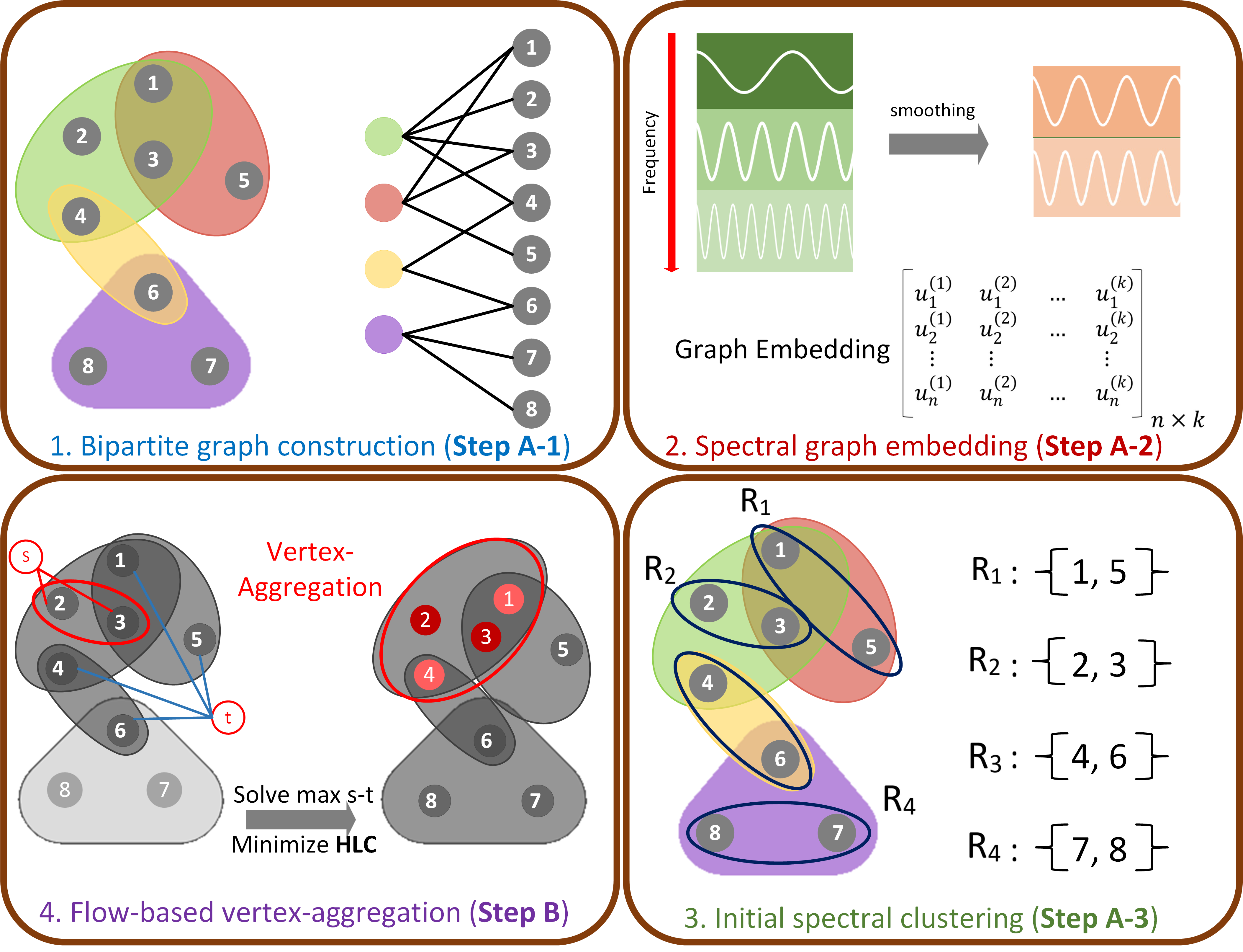
Figure 1: Overview of the proposed HyperSF framework

IV-B Step A: Initial spectral graph clustering

We apply star expansion to model the hypergraph with a pairwise relationship between the vertices so that the eigenvectors of the graph Laplacian matrix can be leveraged for spectral graph embedding (vector representation of vertices). Since we want to cluster highly related vertices in a local neighborhood so that the coarsened graph will preserve the structural properties of the original hypergraph. This requires to approximate the first few (low-frequency) eigenvectors related to the key spectral properties of the graph. To achieve this goal, we leverage the following scalable low-pass filtering algorithm to effectively remove high-frequency graph signal components and subsequently map the each vertex into a $k$-dimensional vector, where $k$ denotes the number of smoothed testing vectors (graph signals).

Let $u$ be a random vector in which each element corresponds to a vertex in the graph. $u$ can be considered as a linear combination of many eigenvectors. Existing iterative methods like Gauss-Seidel and Jacobi relaxation procedures can be leveraged as low-pass graph filters for removing highly oscillating components in $u$, which will produce smoothed vectors that correspond to the linear combination of the first few eigenvectors:

$$u=\Sigma_{i=1}^{n}\gamma_{i}x_{i}\Rightarrow\hat{u}=\Sigma_{i=1}^{\hat{n}}\hat{\gamma_{i}}x_{i}\quad\hat{n}\ll n,$$ (12)

where $\gamma_{i}$ and $\hat{\gamma_{i}}$ are the weighting coefficients, and $\hat{u}$ is the smoothed vector that is obtained after applying a few steps of the Gauss-Seidel iterations on $u$. Applying the above filtering (smoothing) function for $k$ different random vectors (orthogonal to the all-one vector) will result in $k$ smoothed vectors $K=(u^{(1)}...u^{(k)})$ that allow embedding the graph into a $k$-dimensional space. Next, we repeatedly apply spectral clustering for each hyperedge (sorted with descending cardinalities) to find node clusters based on their embedding vectors (smoothed vectors) and the hypergraph coarsening (reduction) ratio. When processing each hyperedge, it is important to flag the nodes that have already been processed, and skip the following hyperedges that include the flagged nodes. Algorithm 1 provides the details of the proposed initial spectral graph clustering scheme (Step A-3 shown in Fig. 1).

Algorithm 1 Initial spectral graph clustering

Input: Hypergraph $H=(V,E)$, $n=\left|V\right|$, $m=\left|E\right|$, and embedding dimension $k$;
Output: A set of vertex clusters $\mathcal{R}$;

1:  Construct the bipartite graph $G$ corresponding to the hypergraph $H$ by applying the star model ;

2:  Generate $k$ different random vector related to $G$;

3:  Perform smoothing function to remove the high frequency components;

4:  Map the graph vertices into a $k$-dimensional space using the smoothed vectors;

5:  Sort the hyperedges according to their cardinality: $|e_{1}|>|e_{2}|>...>|e_{m}|$;

6:  for $i\leftarrow 1$ to $m$ do

7:    $R^{(i)}\leftarrow$ cluster the vertices in $e_{i}$ using $k$-means method;

8:  end for

9:  Return $\mathcal{R}$ .

IV-C Step B: Flow-based hypergraph local clustering

In this section, we improve the quality of the initial spectral graph clustering by incorporating a flow-based low clustering technique [37] for aggregating vertices with minimal impact on the global hypergraph structure.

IV-C1 Flow-based hypergraph clustering

Semi-supervised clustering methods utilize flow-based techniques to find a cluster of vertices strongly connected to the seed nodes $R$, which repeatedly solve max $s$-$t$ flow, min $s$-$t$ cut problem to minimize HLC.

We formalize the hypergraph coarsening problem into a semi-supervised clustering task to aggregate the strongly-connected vertices that allow minimizing (11). To this end, the flow-based clustering method utilizes the output of the initial spectral graph clustering (Algorithm 1) and treats each cluster as a seed node set $R$. For each seed node set, we repeatedly solve a max $s$-$t$ flow, min $s$-$t$ cut problem to decide a set of node clusters that minimizes the localized conductance. To this end, we first create the auxiliary hypergraph by introducing a source vertex $s$ and sink vertex $t$. Next, we replace each hyperedge with a directed graph by creating a network: for each vertex $r\in R$ we introduce an edge $(s,r)$, whereas for each $j\in\hat{R}$ we introduce an edge $(j,t)$; we also introduce two auxiliary vertices (e.g. the green squares shown in Fig. 2) $a$ and $a^{\prime}$ and create a directed edge from $a$ to $a^{\prime}$. In the last, for each vertex $\{v\in e\}_{e\in E}$, we introduce a directed edge $(a,v)$ and a directed edge $(v,a^{\prime})$. We show how to build the directed graph model for a given set of hyperedges in Fig. 2.

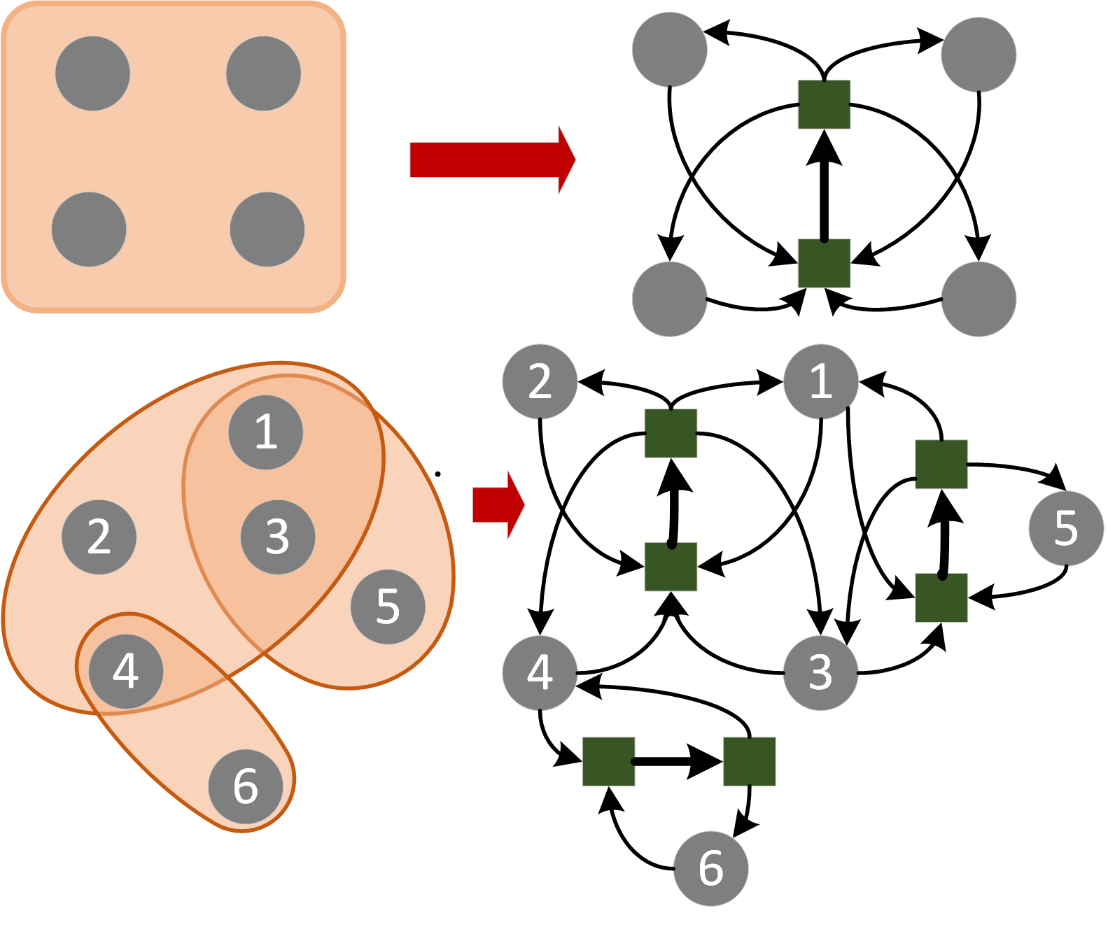
Figure 2: Hypergraph to directed graph conversion

We initialize $S=R$ and iteratively update $S$ to minimize HLC by repeatedly solving the max $s$-$t$ flow, min $s$-$t$ cut problem on the created auxiliary hypergraph to minimize the hypergraph cut [38]:

$$cut^{s-t}(S)=cut_{H}(S)+vol_{H}(\hat{S}\cap R)+\delta vol_{H}(S\cap\hat{R}).$$ (13)

In the last, we aggregate the output set of vertices obtained from flow-based methods that minimize the localized conductance to produce a smaller hypergraph with fewer vertices while preserving the key structural properties of the original hypergraph. We flag the nodes that are already clustered to avoid assigning the same node to different clusters.

IV-C2 Flow-based local clustering

An algorithm is local if the input is a small portion of the original dataset. The aforementioned flow-based hypergraph clustering algorithm can be made strongly local when expanding the network around the seed nodes $R$, which will obviously benefit the proposed hypergraph coarsening framework: (1) applying the max $s$-$t$ flow, min $s$-$t$ cut problem on the local neighborhood of the seed nodes restricts node-aggregation locally and keeps the global hypergraph structure intact; (2) such a local clustering scheme will significantly improve the algorithm efficiency due to the small-scale input dataset.

To achieve flow-based local clustering of hypergraph nodes, we first construct a sub-hypergraph $H_{L}$ by iteratively expanding the hypergraph around the seed node set $R$ and then repeatedly solve the hypergraph cut problem to minimize HLC until no significant changes in local conductance are observed. Let $H=(V,E)$ be the hypergraph. We define $E(S)=\cup_{v\in V,v\in\{e\}_{e\in E}}E(v)$ for any set $S\subseteq V$. We denote $H_{\varsigma}=(V\cup\{s,t\},E\cup E^{st})$, where $E^{st}$ is the terminal edge set. We aim to construct a sub-hypergraph $H_{L}$ to replace $H_{\varsigma}$ that minimizes HLC by repeatedly solving a local version of (13). To this end, we set up an oracle to discover a set of best neighborhood vertices for a given vertex $v$:

$$\kappa(v)=\{u\in V\}_{(u,v)\in e,e\in E}.$$ (14)

We let the oracle accept a set of seed nodes $R$ and return $\kappa(R)=\cup_{v\in R}\kappa(v)$. By utilizing the best neighborhood of the seed nodes $\kappa(R)$, we build a local hypergraph $H_{L}=(V_{L}\cup\{s,t\},E_{L}\cup E_{L}^{st})$, where $V_{L}=R\cup\kappa(R)$ and $E_{L}=\{e\in E\mid V_{L}\in e\}$. We create the local auxiliary hypergraph of $H_{L}$ by introducing the source node $s$ and sink node $t$, so that $E_{L}^{st}\subseteq E^{st}$, and repeatedly solve the max $s$-$t$ flow, min $s$-$t$ cut problem to minimize HLC. The algorithm continuously expands $H_{L}$ and includes more vertices and hyperedges from $H_{\varsigma}$ by solving (13) for the local hypergraph $H_{L}$.

Algorithm 2 Flow-based hypergraph clustering

Input: Hypergraph $H=(V,E)$, $R\subseteq\mathcal{R}$, and $\epsilon$;
Output: A set of vertices $S$ that minimizes HLC(S);

1:  Assign the seed nodes $S\leftarrow R$;

2:  $\Delta_{\textbf{HLC}}\leftarrow\infty$;

3:  while $\Delta_{\textbf{HLC}}>\epsilon$ do

4:    Identify the best neighborhood of seed nodes $\kappa(S)$;

5:    Update $S$ according to $\kappa(S)$ to construct $H_{L}$;

6:    Add a source node $s$ and sink node $t$ to $H_{L}$;

7:    Repeatedly solve the max $s$-$t$ flow, min $s$-$t$ cut problem by minimizing (13) for $H_{L}$;

8:    $\Delta_{\textbf{HLC}}\leftarrow\textbf{HLC(S)}^{j}-\textbf{HLC(S)}^{j-1}$;

9:  end while

10:  Return $S$.

In Algorithm 2 we present the details of the flow based local clustering technique. It accepts the original hypergraph $H=(V,E)$, a set of seed nodes in $R\subseteq\mathcal{R}$, and the convergence parameter $\epsilon$, which will output a set of strongly connected vertices $S$ that minimizes HLC.

IV-D Divide-and-conquer

To further improve the flow-based algorithm efficiency, we leverage a divide-and-conquer approach to partition the dataset into different parts with strongly connected vertices and perform the flow-based method separately in each partition. To this end, we use Metis as a standalone partitioning tool to split the undirected bipartite graph corresponding to the original hypergraph. The flow-based method produces the clusters in a parallel way that expedites the proposed node-aggregation procedure. Additionally, the number of partitions determines the runtime and quality of the algorithm. Our method allows a flexible trade-off between algorithm efficiency and solution accuracy, which can be achieved by adjusting the size of each partition. For example, choosing smaller partitions will result in a higher runtime efficiency but negatively impact hypergraph clustering (coarsening) solution. In Algorithm 3, we illustrate the entire procedure for spectral hypergraph coarsening.

Algorithm 3 The HyperSF algorithm flow

Input: Hypergraph $H=(V,E)$, $n=\left|V\right|$, $m=\left|E\right|$;
Output: Coarsened hypergraph $H_{c}=(V_{c},E)$, where $\left|V_{c}\right|\ll n$;

1:  Call Algorithm 1 to compute $\mathcal{R}$ via spectral embedding of bipartite graph $G$;

2:  $\{p\in V\}_{\subseteq P}\leftarrow$ Apply Metis partitioning to obtain a set of vertices in the same region;

3:  for $j\leftarrow 1$ to $\left|P\right|$ do

4:    $\hat{R}\leftarrow R_{\subseteq\mathcal{R}}\cap\{p\}_{\subseteq P}^{j}$;

5:    for $i\leftarrow 1$ to $\left|\hat{R}\right|$ do

6:       Choose a set of seed nodes $S\leftarrow$ $\hat{R}^{i}$;

7:       $\hat{S}\leftarrow$ Call Algorithm 2 to reach a set of strongly connected vertices;

8:       Aggregate $\{v\in\hat{S}\}_{\hat{S}\subseteq V}$;

9:    end for

10:  end for

11:  Return $H_{c}$, where $\left|V_{c}\right|\ll n$.

IV-E Algorithm complexity of HyperSF

The runtime complexity of Step A for the graph-based spectral clustering is $O(E)$ since we only perform the node clustering within each hyperedge; the runtime complexity of Step B is $O\left(k^{3}vol_{H}(R)^{3}(1+\epsilon^{-1})^{3}\right)$, where $k$ is the maximum hyperedge cardinality. Accordingly, the worst-case runtime complexity of the entire HyperSF algorithm is $O\left(nk^{3}vol_{H}(R)^{3}(1+\epsilon^{-1})^{3}\right)$.

V Experimental Results

We conduct extensive experiments to analyze the performance of the proposed spectral hypergraph coarsening method using a set of VLSI-related datasets “ibm01” to “ibm18” . By testing other hypergraph coarsening techniques on the same data sets, we can provide a fair comparison among different approaches. We have implemented HyperSF in Julia by incorporating the graph spectral embedding technique with the local hypergraph flow-based clustering. All experiments ran on a laptop with 8 GB of RAM and a 2.2 GHz Quad-Core Intel Core i7 processor. An implementation of our algorithm and the code for reproducing our experimental results are available online at https://github.com/aghdaei/HyperSFhttps://github.com/aghdaei/HyperSF.

V-A The results of spectral hypergraph coarsening

We compare the performance of the proposed spectral hypergraph coarsening method (HyperSF) with other hypergraph coarsening frameworks. We compare our algorithm with non-spectral coarsening methods used in hypergraph partitioning methods to investigate our algorithm’s performance thoroughly. To the best of our knowledge, the state-of-the-art hypergraph partitioners leverage heuristic-based hypergraph coarsening frameworks to contract the hyperedges based on edge similarity criteria. In addition, we also construct the bipartite graph of the original hypergraph and use the existing spectral methods to reduce the hypergraph size. We used the average conductance of all clusters to evaluate the performance of HyperSF when comparing with the other hypergraph coarsening algorithms. According to the Cheeger’s inequality, a smaller average conductance implies a better graph coarsening solution.

To this end, we compute the following average local conductance $\Phi$ of the node clusters produced by each method:

$$\Phi=\frac{1}{\left|S\right|}\Sigma_{i=1}^{\left|S\right|}\textbf{HLC}(S^{i}).$$ (15)

V-A1 Spectral methods

Although there is no existing spectral hypergraph coarsening framework to compare with HyperSF, we can apply star and clique models to construct the corresponding undirected bipartite graphs associated with the hypergraph. Once a simple graph is constructed, the traditional spectral graph coarsening methods [17] can be leveraged for aggregating the spectrally-similar vertices and generating a smaller undirected graph. Once the node clusters are produced, we can compute HLC of each node set and thus $\Phi$ for the original hypergraph. Fig. 3 shows the computed average local conductance $\Phi$ of spectral hypergraph coarsening methods for all test sets using the same coarsening ratio. The results show that HyperSF always achieves the lowest $\Phi$ for all the datasets.

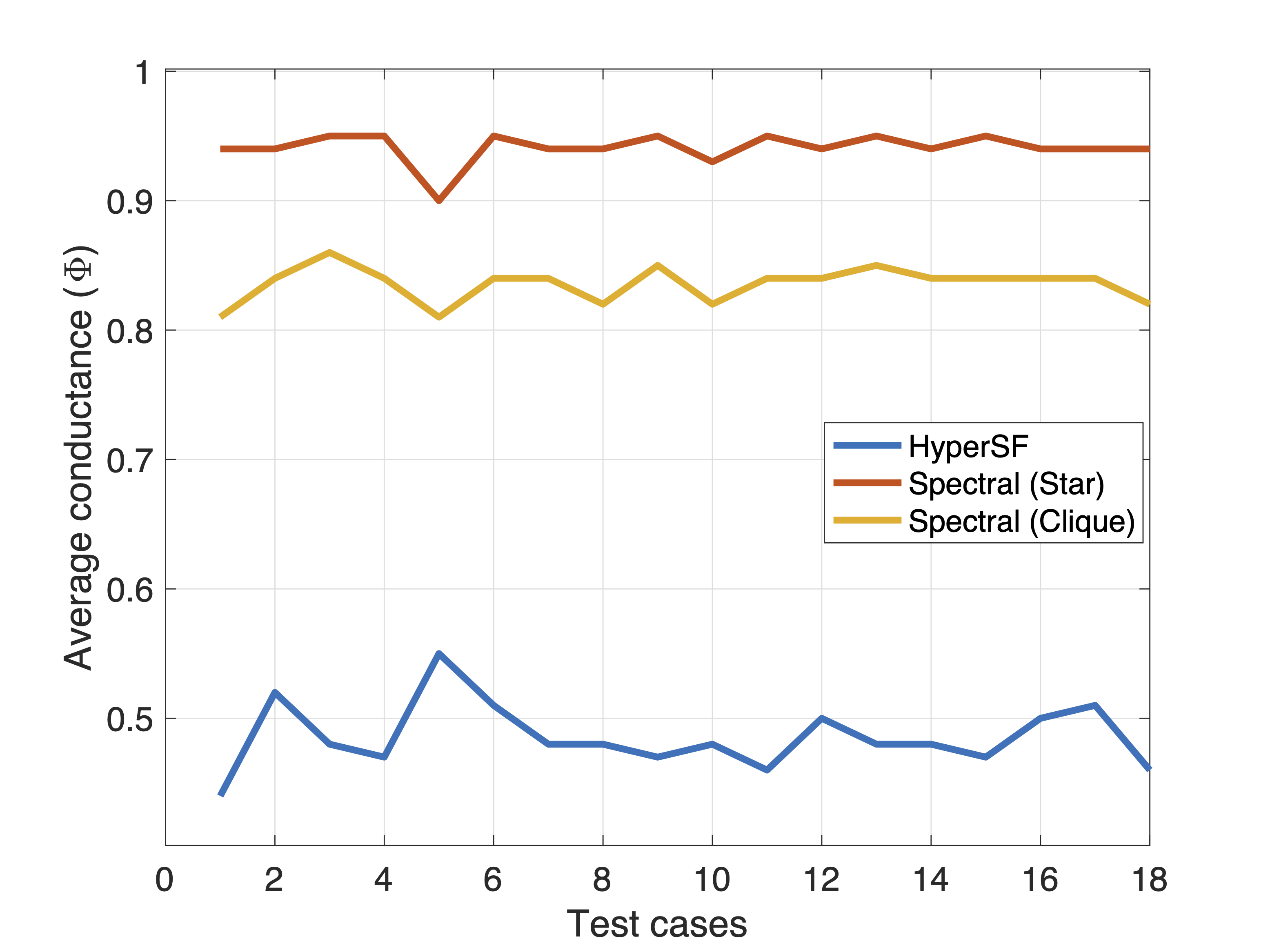
Figure 3: Average conductance ($\Phi$) comparison: HyperSF vs spectral methods using all ibm test cases

V-A2 Non-spectral methods

In this section, we compare the performance of HyperSF with two non-spectral hypergraph coarsening approaches. The first method directly applies Metis on the undirected graphs converted from the original hypergraph (using star and clique expansions) and aggregates the vertices within each partition to create a smaller hypergraph. The second method utilizes a popular hypergraph partitioning tool, Hmetis, to aggregate strongly-connected vertices in each partition. To provide a fair comparison, we apply the same coarsening ratio in different methods such that all coarsened hypergraphs $H_{s}=(V_{s},E_{s})$ will have the same size $\left|V_{s}\right|$. In Fig. 4, we show the performance of Metis (using star and clique models), Hmetis, and HyperSF by computing the average local conductance $\Phi$ for all test cases. We observe that HyperSF always achieves significantly better coarsening results.

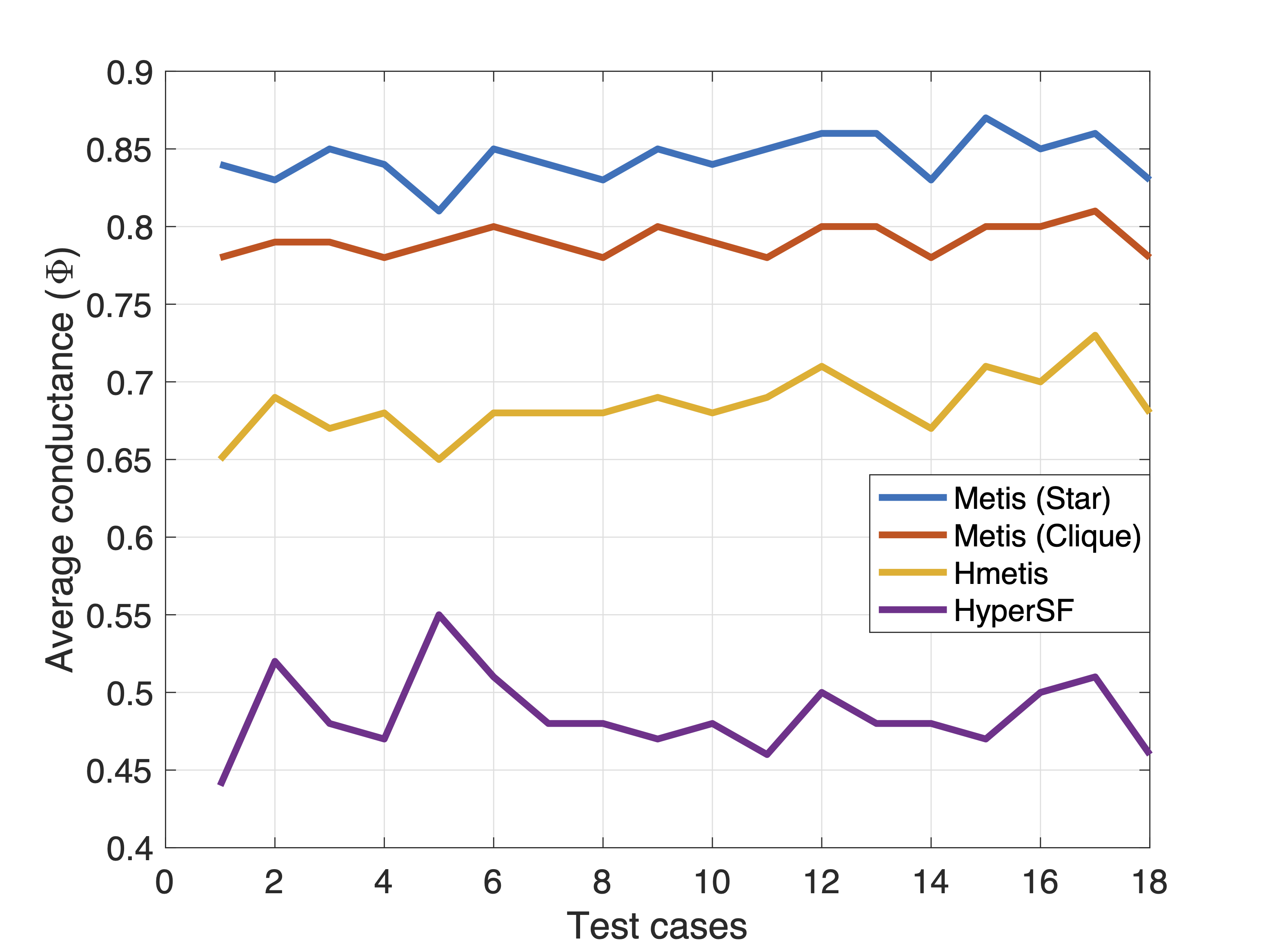
Figure 4: Average conductance ($\Phi$) comparison: HyperSF vs non-spectral methods using all ibm test cases

TABLE I: The average local conductance ($\Phi$) comparison between HyperSF and other coarsening methods

Hypergraphs	V	E	RR (%)	Spectral ($\mathcal{S}$)	Spectral ($\mathcal{C}$)	Metis ($\mathcal{S}$)	Metis ($\mathcal{C}$)	Hmetis	HyperSF
ibm01	12752	14111	75	0.94	0.81	0.84	0.78	0.65	0.44
ibm02	19601	19584	75	0.94	0.84	0.83	0.79	0.69	0.52
ibm03	23136	27401	75	0.95	0.86	0.85	0.79	0.67	0.48
ibm04	27507	31970	75	0.95	0.84	0.84	0.78	0.68	0.47
ibm05	29347	28446	75	0.90	0.81	0.81	0.79	0.65	0.55
ibm06	32498	34826	75	0.95	0.84	0.85	0.80	0.68	0.51
ibm07	45926	48117	75	0.94	0.84	0.84	0.79	0.68	0.48
ibm08	51309	50513	75	0.94	0.82	0.83	0.78	0.68	0.48
ibm09	53395	60902	75	0.95	0.85	0.85	0.80	0.69	0.47
ibm10	69429	75196	75	0.93	0.82	0.84	0.79	0.68	0.48
ibm11	70558	81454	75	0.95	0.84	0.85	0.78	0.69	0.46
ibm12	71076	77240	75	0.94	0.84	0.86	0.80	0.71	0.50
ibm13	84199	99666	75	0.95	0.85	0.86	0.80	0.69	0.48
ibm14	147605	152772	75	0.94	0.84	0.83	0.78	0.67	0.48
ibm15	161570	186608	75	0.95	0.84	0.87	0.80	0.71	0.47
ibm16	183484	190048	75	0.94	0.84	0.85	0.80	0.70	0.50
ibm17	185495	189581	75	0.94	0.84	0.86	0.81	0.73	0.51
ibm18	210613	201920	75	0.94	0.82	0.83	0.78	0.68	0.46

TABLE I shows the average local conductance $\Phi$ of different methods using the same hypergraph reduction ratio (RR). We reduce the number of nodes in each original hypergraph by $75\%$ (e.g., for a hypergraph with $100$ nodes, the coarsened hypergraph will have only $25$ nodes). For simplicity, we denote the star and clique models by $\mathcal{S}$ and $\mathcal{C}$, respectively. The experimental results confirm that HyperSF can significantly improve the average local conductance compared with other hypergraph coarsening methods for all test cases.

V-B Cut preservation after hypergraph coarsening

To further evaluate the performance of the proposed hypergraph coarsening algorithm, we calculate the cut before and after coarsening. Before coarsening: Hmetis bisects the original hypergraph into two partitions and returns the number of hyperedges intersecting between two partitions; after coarsening: HyperSF first produces a smaller hypergraph that is used as the input of Hmetis; then the node partitioning results are mapped back to the original hypergraph for computing the cut. Fig. 5 shows the cuts before and after applying HyperSF using various reduction ratios (RRs) for the dataset “ibm01”. While Hmetis bisects the original hypergraph by cutting $182$ hyperedges, only $2\%$-$3\%$ relative difference in cut is observed when bisecting the coarsened hypergraph, which implies the coarsened hypergraphs obtained using HyperSF can very well preserve the original cut.

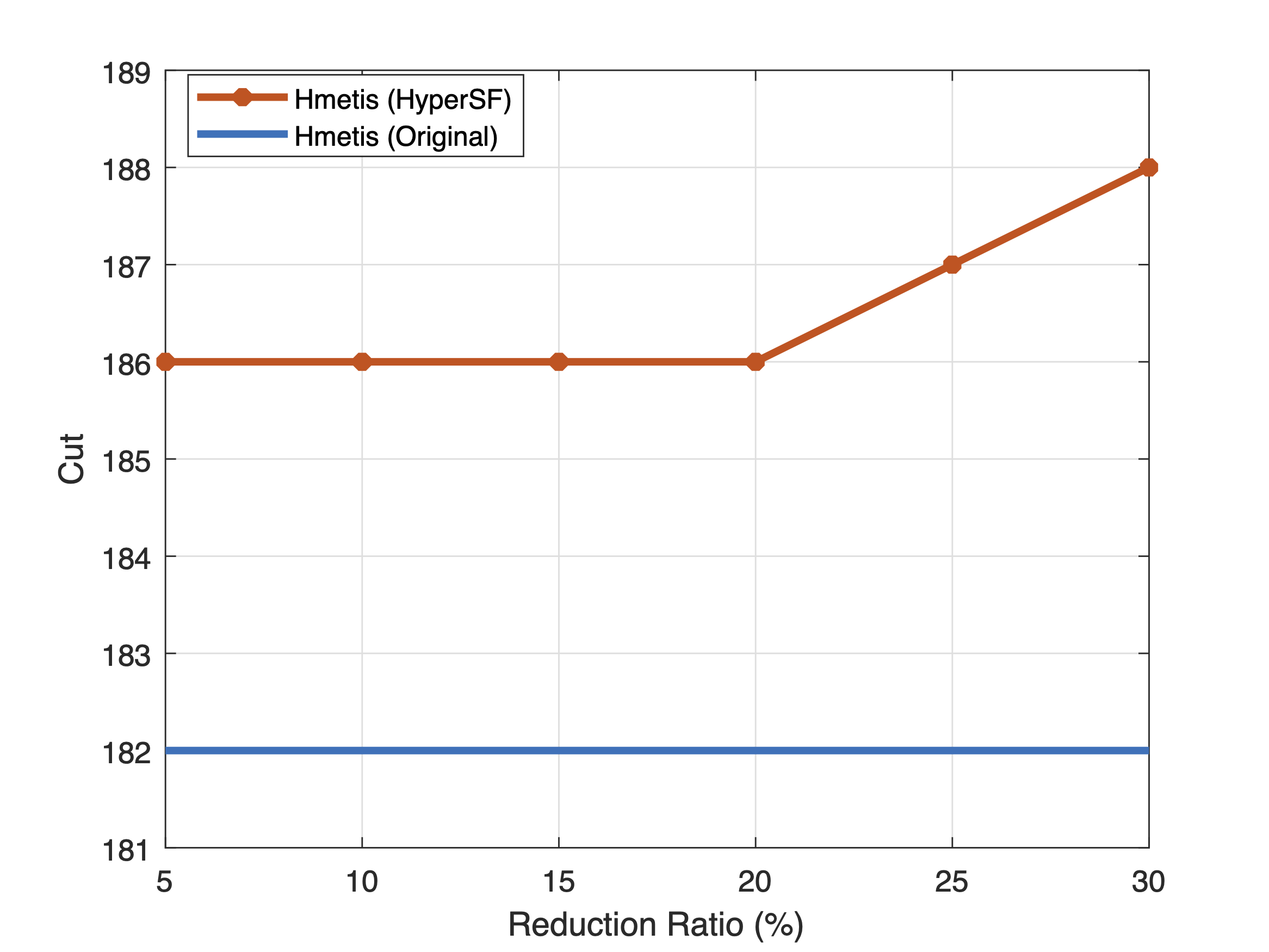
Figure 5: Cut preservation after hypergraph coarsening

V-C Hypergraph k-way partitioning

The goal of this experiment is to study the performance of the proposed algorithm for k-way hypergraph partitioning tasks. We use HyperSF as a standalone hypergraph partitioner and Hmetis as the baseline to evaluate the performance and efficiency. HyperSF aims to aggregate the spectrally-similar vertices to preserve the structural properties of the original hypergraph by ignoring the criteria heavily used in modern balanced partitioning methods. For example, Hmetis iteratively bisects the hypergraph and minimizes the hypergraph cut for achieving a balanced partitioning result. To achieve a fair comparison of hypergraph partitioning between HyperSF and Hmetis, we consider an imbalance parameter (UBfactor) that is defined to be the upper bound of the ratio between the maximum volume and the average volume. For instance, given UBfactor$=9$ and $Nparts=4$ for partitioning a hypergraph with $n$ vertices, the partitioner will produce a set of partitions so that the ratio between the maximum volume and the average volume will be bounded by $1.09\times n/4$. We restrict the size of each partition by including UBfactor to HyperSF, which will effectively set a limit on the size of each partition: if a vertex intends to join a partition with full capacity, it will be assigned to the nearest partition by measuring the Euclidean distance between that node and its neighborhood partition. However, adding UBfactor will inevitably impact the solution quality due and lead to increased HLC.

Since the partitions are no longer strictly balanced, the cut objective will not be meaningful for assessing the performance. Consequently, we use the $k$-way conductance as the metric to compare the performance of both methods. The $k$-way conductance can be computed by finding the maximum (node cluster) conductance over all partitions [39]. Fig. 6 shows the result of conducting a hypergraph $k$-way partitioning on the “ibm01” dataset to compute the $k$-way conductance with Hmetis and HyperSF. Both hypergraph partitioners split the vertices into $Nparts=\left[630,750,835,970\right]$ through multiple experiments and imposed the same imbalance factor between the partitions. We observe a smaller $k$-way conductance when using HyperSF compared to Hmetis for various partitioning and imbalance parameter settings.

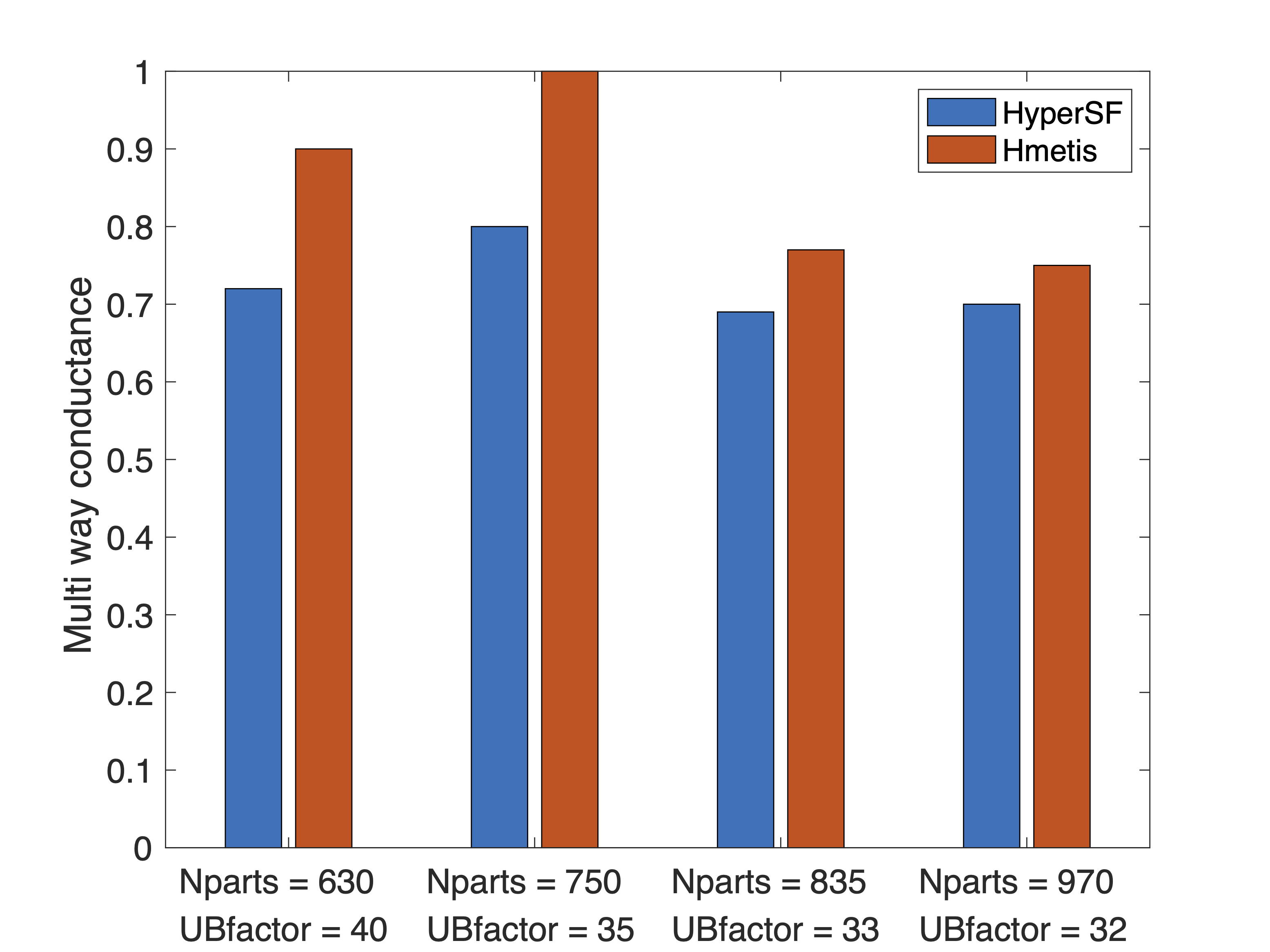
Figure 6: K-way conductance analysis for different number of partitions with respect to the imbalance parameter

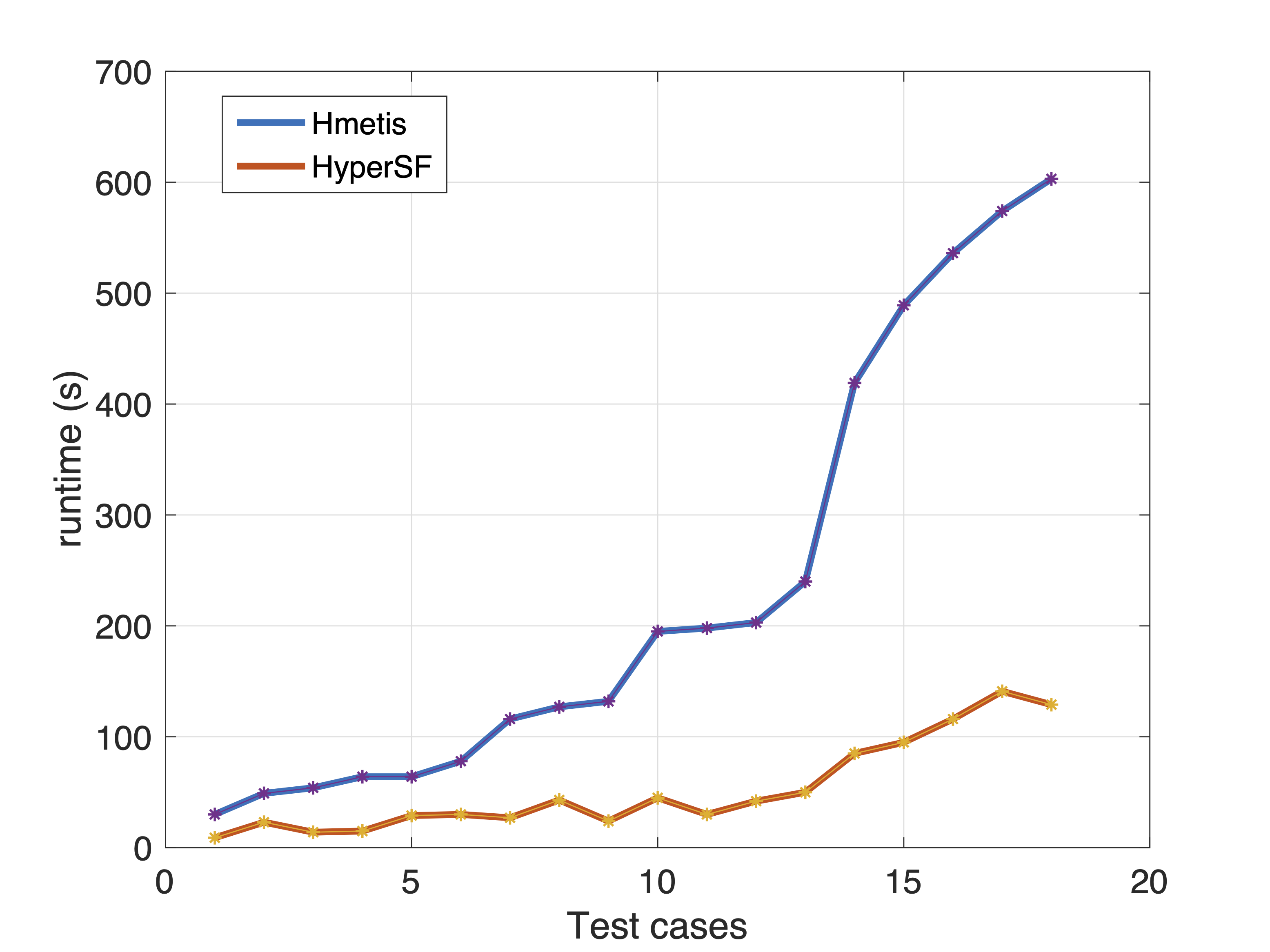
Figure 7: Runtime comparison for all test cases

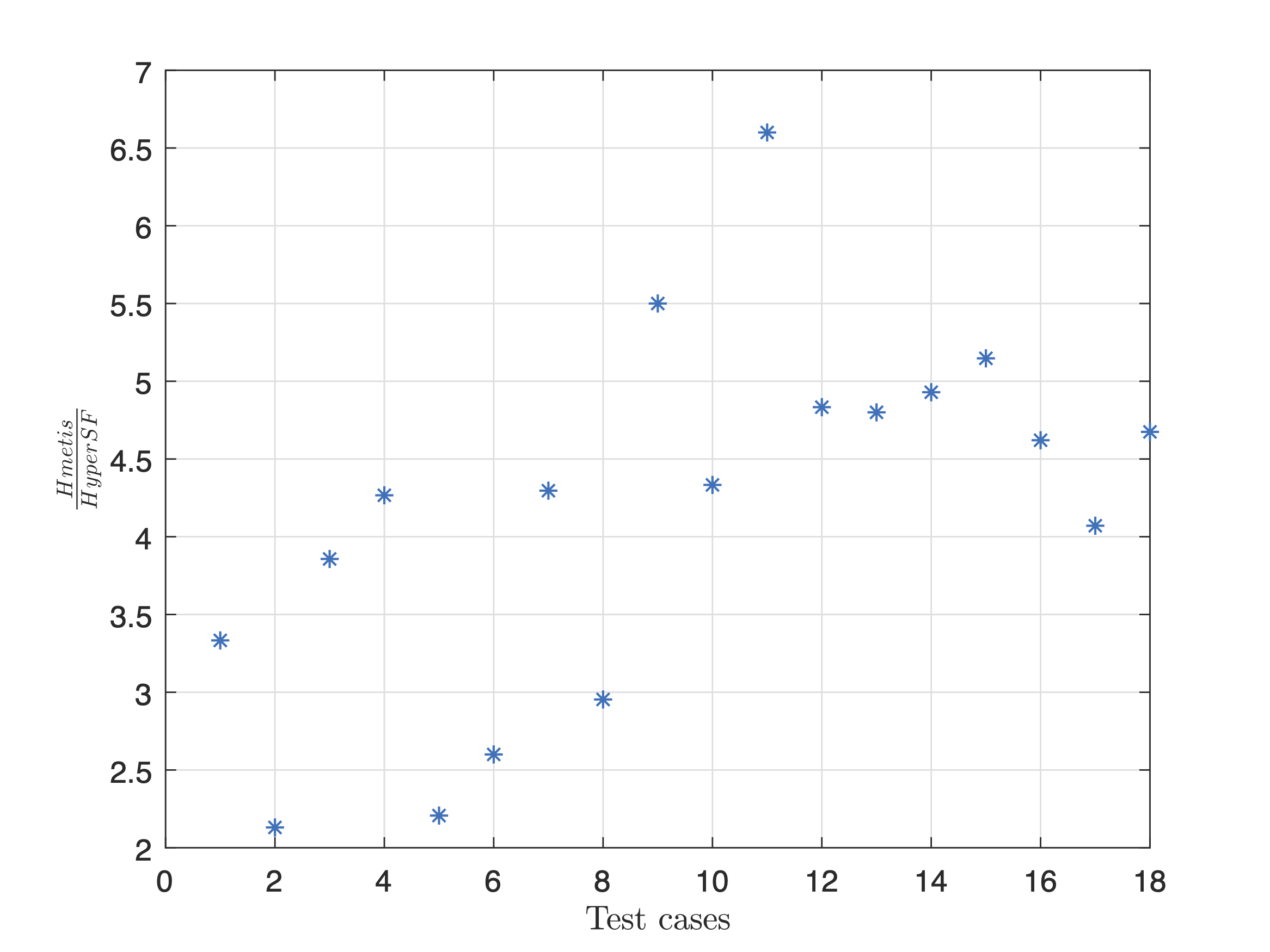
Figure 8: Runtime speedups for all test cases

V-D Runtime analysis

We compared the runtime of HyperSF with Hmetis for all the test cases to evaluate the algorithm scalability. As shown in Fig. 7, the gap between the Hmetis and HyperSF keeps increasing as the hypergraph sizes increase. Fig. 8 shows up to $6.6\times$ runtime speedup achieved by HyperSF, which further highlights the superior runtime efficiency of HyperSF over Hmetis.

VI Conclusion

In this work, we propose an efficient spectral hypergraph coarsening algorithm (HyperSF) for aggressively reducing the size of hypergraphs without impacting the key spectral (structural) properties. Our approach leverages an initial spectral clustering procedure and a flow-based local clustering scheme for detecting the sets of strongly-coupled hypergraph vertices. Our results for a variety of hypergraphs extracted from real-world VLSI design benchmarks show that the proposed HyperSF can significantly improve the solution quality and runtime efficiency when compared with prior state-of-the-art hypergraph coarsening algorithms.

References

- [1] Y. Jin, A. Loukas, and J. JaJa, “Graph coarsening with preserved spectral properties,” in International Conference on Artificial Intelligence and Statistics. PMLR, 2020, pp. 4452–4462.
- [2] M. Fahrbach, G. Goranci, R. Peng, S. Sachdeva, and C. Wang, “Faster graph embeddings via coarsening,” in International Conference on Machine Learning. PMLR, 2020, pp. 2953–2963.
- [3] B. F. Auer and R. H. Bisseling, “Graph coarsening and clustering on the gpu.” Graph Partitioning and Graph Clustering, vol. 588, p. 223, 2012.
- [4] I. Safro, P. Sanders, and C. Schulz, “Advanced coarsening schemes for graph partitioning,” Journal of Experimental Algorithmics (JEA), vol. 19, pp. 1–24, 2015.
- [5] F. M. Bianchi, D. Grattarola, and C. Alippi, “Spectral clustering with graph neural networks for graph pooling,” in International Conference on Machine Learning. PMLR, 2020, pp. 874–883.
- [6] A. B. Kahng, J. Lienig, I. L. Markov, and J. Hu, VLSI physical design: from graph partitioning to timing closure. Springer Science & Business Media, 2011.
- [7] Z. Liu, B. Xiang, W. Guo, Y. Chen, K. Guo, and J. Zheng, “Overlapping community detection algorithm based on coarsening and local overlapping modularity,” IEEE Access, vol. 7, pp. 57 943–57 955, 2019.
- [8] G. Karypis and V. Kumar, “A fast and high quality multilevel scheme for partitioning irregular graphs,” SIAM Journal on scientific Computing, vol. 20, no. 1, pp. 359–392, 1998.
- [9] O. E. Livne and A. Brandt, “Lean algebraic multigrid (lamg): Fast graph laplacian linear solver,” SIAM Journal on Scientific Computing, vol. 34, no. 4, pp. B499–B522, 2012.
- [10] D. Ron, I. Safro, and A. Brandt, “Relaxation-based coarsening and multiscale graph organization,” Multiscale Modeling & Simulation, vol. 9, no. 1, pp. 407–423, 2011.
- [11] Y. Ma, S. Wang, C. C. Aggarwal, and J. Tang, “Graph convolutional networks with eigenpooling,” in Proceedings of the 25th ACM SIGKDD International Conference on Knowledge Discovery & Data Mining, 2019, pp. 723–731.
- [12] A. Loukas and P. Vandergheynst, “Spectrally approximating large graphs with smaller graphs,” in International Conference on Machine Learning. PMLR, 2018, pp. 3237–3246.
- [13] A. Loukas, “Graph reduction with spectral and cut guarantees.” Journal of Machine Learning Research, vol. 20, no. 116, pp. 1–42, 2019.
- [14] F. Dorfler and F. Bullo, “Kron reduction of graphs with applications to electrical networks,” IEEE Transactions on Circuits and Systems I: Regular Papers, vol. 60, no. 1, pp. 150–163, 2012.
- [15] M. Purohit, B. A. Prakash, C. Kang, Y. Zhang, and V. Subrahmanian, “Fast influence-based coarsening for large networks,” in Proceedings of the 20th ACM SIGKDD international conference on Knowledge discovery and data mining, 2014, pp. 1296–1305.
- [16] G. Bravo Hermsdorff and L. Gunderson, “A unifying framework for spectrum-preserving graph sparsification and coarsening,” Advances in Neural Information Processing Systems, vol. 32, pp. 7736–7747, 2019.
- [17] Z. Zhao, Y. Zhang, and Z. Feng, “Towards scalable spectral embedding and data visualization via spectral coarsening,” in Proceedings of the 14th ACM International Conference on Web Search and Data Mining, 2021, pp. 869–877.
- [18] Y. Lin, Z. Jiang, J. Gu, W. Li, S. Dhar, H. Ren, B. Khailany, and D. Z. Pan, “Dreamplace: Deep learning toolkit-enabled gpu acceleration for modern vlsi placement,” IEEE Transactions on Computer-Aided Design of Integrated Circuits and Systems, 2020.
- [19] G. Lee, J. Ko, and K. Shin, “Hypergraph motifs: Concepts, algorithms, and discoveries,” arXiv preprint arXiv:2003.01853, 2020.
- [20] G. Karypis, R. Aggarwal, V. Kumar, and S. Shekhar, “Multilevel hypergraph partitioning: Application in vlsi domain,” in Proceedings of the 34th Annual Design Automation Conference, ser. DAC ’97. New York, NY, USA: Association for Computing Machinery, 1997, p. 526–529. [Online]. Available: https://doi.org/10.1145/266021.266273
- [21] K. Devine, E. Boman, R. Heaphy, R. Bisseling, and U. Catalyurek, “Parallel hypergraph partitioning for scientific computing,” in Proceedings 20th IEEE International Parallel Distributed Processing Symposium, 2006, pp. 10 pp.–.
- [22] B. Vastenhouw and R. H. Bisseling, “A two-dimensional data distribution method for parallel sparse matrix-vector multiplication,” SIAM Rev., vol. 47, no. 1, p. 67–95, Jan. 2005. [Online]. Available: https://doi.org/10.1137/S0036144502409019
- [23] S. Agarwal, K. Branson, and S. Belongie, “Higher order learning with graphs,” in Proceedings of the 23rd International Conference on Machine Learning, ser. ICML ’06. New York, NY, USA: Association for Computing Machinery, 2006, p. 17–24. [Online]. Available: https://doi.org/10.1145/1143844.1143847
- [24] D. Zhou, J. Huang, and B. Schölkopf, “Learning with hypergraphs: Clustering, classification, and embedding,” vol. 19, 01 2006, pp. 1601–1608.
- [25] T.-H. H. Chan, A. Louis, Z. G. Tang, and C. Zhang, “Spectral properties of hypergraph laplacian and approximation algorithms,” J. ACM, vol. 65, no. 3, Mar. 2018. [Online]. Available: https://doi.org/10.1145/3178123
- [26] T.-H. H. Chan and Z. Liang, “Generalizing the hypergraph laplacian via a diffusion process with mediators,” Theoretical Computer Science, vol. 806, pp. 416–428, 2020.
- [27] R. Shaydulin, J. Chen, and I. Safro, “Relaxation-based coarsening for multilevel hypergraph partitioning,” Multiscale Modeling and Simulation, vol. 17, no. 1, p. 482–506, Jan 2019. [Online]. Available: http://dx.doi.org/10.1137/17M1152735
- [28] Ü. V. Çatalyürek and C. Aykanat, “Patoh (partitioning tool for hypergraphs),” in Encyclopedia of Parallel Computing. Springer, 2011, pp. 1479–1487.
- [29] L. Hagen and A. Kahng, “New spectral methods for ratio cut partitioning and clustering,” IEEE Transactions on Computer-Aided Design of Integrated Circuits and Systems, vol. 11, no. 9, pp. 1074–1085, 1992.
- [30] T. Soma and Y. Yoshida, “Spectral sparsification of hypergraphs,” in Proceedings of the Thirtieth Annual ACM-SIAM Symposium on Discrete Algorithms. SIAM, 2019, pp. 2570–2581.
- [31] S. Fu, W. Liu, Y. Zhou, and L. Nie, “Hplapgcn: Hypergraph p-laplacian graph convolutional networks,” Neurocomputing, vol. 362, pp. 166–174, 2019.
- [32] H. H. Yang and D. Wong, “Efficient network flow based min-cut balanced partitioning,” in The Best of ICCAD. Springer, 2003, pp. 521–534.
- [33] L. Orecchia and Z. A. Zhu, “Flow-based algorithms for local graph clustering,” in Proceedings of the twenty-fifth annual ACM-SIAM symposium on Discrete algorithms. SIAM, 2014, pp. 1267–1286.
- [34] V. Satuluri and S. Parthasarathy, “Scalable graph clustering using stochastic flows: applications to community discovery,” in Proceedings of the 15th ACM SIGKDD international conference on Knowledge discovery and data mining, 2009, pp. 737–746.
- [35] N. Veldt, C. Klymko, and D. F. Gleich, “Flow-based local graph clustering with better seed set inclusion,” in Proceedings of the 2019 SIAM International Conference on Data Mining. SIAM, 2019, pp. 378–386.
- [36] F. R. Chung and F. C. Graham, Spectral graph theory. American Mathematical Soc., 1997, no. 92.
- [37] N. Veldt, A. R. Benson, and J. Kleinberg, “Minimizing localized ratio cut objectives in hypergraphs,” in Proceedings of the 26th ACM SIGKDD International Conference on Knowledge Discovery & Data Mining, 2020, pp. 1708–1718.
- [38] ——, “Hypergraph cuts with general splitting functions,” arXiv preprint arXiv:2001.02817, 2020.
- [39] J. R. Lee, S. O. Gharan, and L. Trevisan, “Multiway spectral partitioning and higher-order cheeger inequalities,” Journal of the ACM (JACM), vol. 61, no. 6, pp. 1–30, 2014.