Mock HUBS observations of hot gas with IllustrisTNG

Abstract

The lack of adequate X-ray observing capability is seriously impeding the progress in understanding the hot phase of circumgalactic medium (CGM), which is predicted to extend to the virial radius of a galaxy or beyond, and thus in acquiring key boundary conditions for studying galaxy evolution. To this end, the Hot Universe Baryon Surveyor (HUBS) is proposed. HUBS is designed to probe hot CGM by detecting its emission or absorption lines with a non-dispersive X-ray spectrometer of high resolution and high throughput. The spectrometer consists of a $60\times 60$ array of microcalorimeters, with each detector providing an energy resolution of $2~{}\mathrm{eV}$, and is placed in the focal plane of an X-ray telescope of $1\degr$ field-of-view. With such a design, the spectrometer is highly optimized for detecting X-ray-emitting hot gas in the CGM of local galaxies, as well as in intra-group medium (IGrM), intra-cluster medium (ICM), or intergalactic medium (IGM). To assess the scientific potential of HUBS, in this work, we created mock observations of galaxies, groups, and clusters at different redshifts with the IllustrisTNG simulation. Focusing exclusively on emission studies, we took into account the effects of light cone, Galactic foreground emission, and background AGN contribution in the mock observations. From the observations, we made mock X-ray images and spectra, analyzed them to derive the properties of the emitting gas in each case, and compared the results with the input parameters from the simulation. The results show that HUBS is well suited for studying hot CGM at low redshifts. The redshift range is significantly extended for measuring IGrM and ICM. The sensitivity limits are also presented for detecting extended emission of low surface brightness.

1 Introduction

Our understanding of galaxies has evolved significantly over the past decade or so. Stimulated by multi-wavelength observations and theoretical studies, we began to view a disc galaxy in terms of a complex ecosystem (see 2017ARA&A..55..389T, , for a recent review): gas in the disc may be heated and expelled into the halo, likely through the action of stellar and/or supermassive black hole feedback, and may subsequently cool and condense in the halo, and eventually, together with newly accreted gas from the larger-scale inter-galactic medium (IGM), fall back onto the disc, providing cold gas for fueling the formation of the next-generation of stars. Though varying in details, such a cycling of baryonic matter between the disc and halo has become a fairly generic feature in theoretical models, but is still seeking observational confirmation. The studies of circum-galactic medium (CGM) have gained significant momentum in recent years, but there are still many unresolved issues remaining, which impede the progress in our understanding of galaxy evolution.

Hydrodynamical simulations show that the CGM is inherently multi-phase, which has also found significant observational support. But, exactly how different phases of the CGM are mixed and distributed is still a matter of much debate, due to the lack of relevant observations, especially X-ray observations that probe the hot phase, which is predicted to be very extended spatially. The observations of edge-on galaxies have established the presence of X-ray-emitting gas in the halo (e.g. 2001ApJ…555L..99W, ; 2004ApJS..151..193S, ; 2006A&A…448…43T, ; 2013MNRAS.435.3071L, ; 2017ApJS..233…20L, ), but only on scales of the order $10~{}\mathrm{kpc}$, which are quite small when compared with virial radii of typically $200\text{--}300~{}\mathrm{kpc}$. If such hot gas extends up to the virial radius of galaxies or beyond, as some models suggest, it could help solve the problem of baryon deficit in galaxies like the Milky Way (e.g. 2011ApJ…737…22A, ; 2012ApJ…755..107D, ; 2017ApJ…850…98B, ), and also provide the boundary conditions necessary for understanding the physics of feedback and physical processes in the CGM.

Directly observing X-ray emission from the CGM is challenging, especially in the outer part, as the density (and thus the emission measure) is likely quite low. On the other hand, for an optically-thin, collisionally-ionized plasma, the emission spectrum is expected to be dominated by lines, so high-resolution X-ray spectroscopy could be an effective way to extend the reach of CGM studies. In this context, the Hot Universe Baryon Surveyor (HUBS) mission was proposed (2020JLTP..199..502C ; see updates in 2020SPIE11444E..2SC ). HUBS aims at filling an void in the detection of X-ray emission from the hot phase of the CGM by employing a non-dispersive X-ray spectrometer of high spectral resolution and high throughput. In this work, we assess the scientific capabilities of HUBS related to the studies of CGM, as well as of hot gas in galaxy groups or clusters, with mock observations.

The paper is structured as follows: In Section 2, we provide a brief description of the HUBS mission, followed by a detailed description of the methodology for creating mock X-ray observations in Section 3. The results from analyzing the mock observations of galaxies, groups, and clusters are shown in Section 4. We discuss the results and conclude in Section 5.

2 The HUBS payload

The design of the HUBS payload is highly optimized for the detection of extended X-ray emission of low surface brightness 2020SPIE11444E..2SC . It puts a strong emphasis on the softest X-ray band (below about $1~{}\mathrm{keV}$), in which the emission lines of the hot CGM are expected to be mainly located, but extends the spectral coverage to about $2~{}\mathrm{keV}$. The X-ray focusing optics employed features a large field-of-view (FoV) to maximize the throughput of detecting diffuse X-ray emission, which is often quantified by the product of the effective area and FoV (often referred to as $\it grasp$). At the focal plane of the optics lies an array of microcalorimeters, which are based on the technology of superconducting transition-edge sensors, with their quantum efficiency (QE) and energy resolution optimized for operating at below $1~{}\mathrm{keV}$. A sub-array of smaller detectors are placed at the centre of the main detector array, providing even higher energy resolution. Such a hybrid design of the detector array is adopted to enhance absorption-line observations of bright background (point) sources. The key parameters of the HUBS payload are summarized in (2020SPIE11444E..2SC, , Table 1).

The throughput of the system is not only determined by the collecting area of X-ray optics, but also by the transmission coefficients of the blocking filters and by the QE of the detectors. The blocking filters are placed in front of the detector array to reject photons at long wavelengths, primarily infrared and optical photons, and thus to reduce shot noise, which would degrade the energy resolution of the detectors. For this work, the collecting area adopted is based on a preliminary design of the optics, as provided by the optics development team (Z.-S. Wang, private communication). To take into account optical vignetting, we averaged the data over a range of off-axis angles up to $30\arcmin$ at each X-ray energy, to derive the FoV-averaged collecting area curve. We note that efforts are being made by the optics development team to further improve the performance of the optics below $1~{}\mathrm{keV}$.

As for the response of the filters, we adopted the measured transmission curve of the blocking filters used by the XQC sounding rocket experiment (D. McCammon, private communication; also see 2002ApJ…576..188M ). Deviating from the five-filter system of XQC, we plan to use six filters in HUBS, with the outermost one located at room temperatures for minimizing contamination of the filter/detector system, so we scaled the XQC filter transmission curve accordingly. Here, we assumed a detector QE of unity.

For creating mock observations, we ignored detector background caused by energetic charged particles in the space environment. This is justified by the fact that HUBS is designed to operate in a low-earth orbit, where the particle background is relatively low, especially in the soft X-ray band that HUBS covers, and is expected to be negligible compared with the X-ray background of cosmic origin (see Sec. 3.4). Multiplying the collecting area of the optical system and the transmission of the filters, we computed the overall effective area of the system, as shown in Fig. 1. Then, we generated the corresponding ancillary response file (ARF), as well as a response matrix file (RMF), for subsequent spectral analyses. For the RMF, we divided the HUBS passing band ($0.1\text{--}2~{}\mathrm{keV}$) into $9500$ pulse height channels (with each $0.2~{}\mathrm{eV}$ in width). The line response of the detector was taken to be of Gaussian shape with its full-width-at-half-maximum (FWHM) set at $2~{}\mathrm{eV}$. Note that we have neglected the difference of the central sub-array of detectors in this work, as we focus exclusively on emission lines.

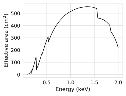
Figure 1: Preliminary effective area of HUBS, as a function of X-ray energy. The effects of optical vignetting have been considered (see text).

3 Mock observation

The procedure for producing mock X-ray observations is similar to that of past studies (e.g., 2003PASJ…55..879Y ; 2005ApJ…623..612F ; 2012MNRAS.424.1012R ; 2020ApJ…893L..24O ).

3.1 Cosmological simulation

We utilized data from the IllustrisTNG simulation ( Marinacci_et_al.(2018) ; Naiman_et_al.(2018) ; Nelson_et_al.(2018) ; Nelson_et_al.(2019a) ; Pillepich_et_al.(2018b) ; Springel_et_al.(2018) ), which was carried out using an advanced moving-mesh code arepo Springel(2010) . For making mock observations, we made use of the full-physics run (TNG100), which has a cubic box volume of $(110.7\ \mathrm{Mpc})^{3}$, a mass resolution of $1.4\times 10^{6}\ {\rm M_{\sun}}$ and $7.5\times 10^{6}\ {\rm M_{\sun}}$ for the baryonic and dark matter, respectively, and a gravitational softening length of $0.5\ h^{-1}\,\mathrm{kpc}$. Galaxies hosted by their dark matter haloes were identified with the subfind algorithm Springel_et_al.(2001) ; Dolag_et_al.(2009) . The simulation adopted the Planck cosmology parameters under the assumption of a flat universe geometry Planck_Collaboration(2016) : a matter density of $\Omega_{\rm m}=0.3089$ (with a baryonic density of $\Omega_{\rm b}=0.0486$), a cosmological constant of $\Omega_{\Lambda}=0.6911$, and a Hubble constant $h=\left.H_{0}\right/\left(100\ {\rm km\,s}^{-1}\,{\rm Mpc^{-1}}\right)=0.6774$. This cosmology was also assumed throughout this work.

3.2 Target selection

Because the spectral coverage of HUBS is limited to the soft X-ray band, it primarily targets on the hot phase of the CGM, as well as hot gas in the intra-group medium (IGrM) or in the outskirts of the intra-cluster medium (ICM), as well as in the filamentary structures. For this work, we selected Friends-of-Friends 1985ApJ…292..371D haloes in the TNG100 simulation at three mass scales, including galaxies ($10^{12}~{}\mathrm{M_{\sun}}<M<10^{13}~{}\mathrm{M_{\sun}}$), galaxy groups ($10^{13}~{}\mathrm{M_{\sun}}<M<10^{14}~{}\mathrm{M_{\sun}}$), and galaxy clusters ($M>10^{14}~{}\mathrm{M_{\sun}}$). To characterize the spatial extent of the dark matter halo of a target source, we define its virial radius as the radius of a sphere in which the mean density is equal to $200$ times the critical density of the universe ($r_{200}$). To separate the central region of the halo from its outskirt, we have further defined a fiducial radius $r_{500}$ in a similar manner.

After going through the snapshots that cover the redshift range of interest, we found many candidate haloes corresponding to the three mass scales for galaxies, galaxy groups, and galaxy clusters. For simplicity, we selected relatively isolated dark matter haloes at each mass scale for three redshifts ($z=0.03$, $0.11$, and $0.27$). The properties of the targets are summarized in Table 3.2. The corresponding X-ray emissivity maps of the targets were computed and are shown in Fig. 2. Note that the redshift of a target is set to be that of the snapshot in which it is located.

As a caveat, we note that the observed metallicity in rich clusters stays nearly constant around $0.2-0.4Z_{\sun}$ outside $\sim 0.15r_{200}$ (e.g., Simionescu2011 ; Gastaldello2021 ). For comparison, we made metallicity profiles for $16$ TNG100 cluster samples at $z=0$ and averaged them to arrive at a profile typical of simulated clusters. The average profile shows that the metalicity decreases towards the outskirt and reaches about $0.2Z_{\sun}$ at $r_{200}$, which is lower than the observed values. This suggests that real systems might be brighter in metal emission lines than the simulated ones.

Table 1: Properties of the selected targets^†

Target	Redshift	Mass	$M_{200}$	$r_{200}$	Type
ID		$\left(\mathrm{M_{\sun}}\right)$	$\left(\mathrm{M_{\sun}}\right)$	$\left(\mathrm{Mpc}\right)$
A	$0.03$	$1.29\times 10^{14}$	$1.16\times 10^{14}$	$1.02$	cluster
B	$0.03$	$5.57\times 10^{13}$	$5.12\times 10^{13}$	$0.77$	group
C	$0.03$	$3.06\times 10^{12}$	$1.98\times 10^{12}$	$0.26$	galaxy
D	$0.11$	$3.78\times 10^{14}$	$3.21\times 10^{14}$	$1.39$	cluster
E	$0.11$	$7.00\times 10^{13}$	$5.95\times 10^{13}$	$0.79$	group
F	$0.11$	$5.23\times 10^{12}$	$4.60\times 10^{12}$	$0.34$	galaxy
G	$0.27$	$2.05\times 10^{14}$	$1.77\times 10^{14}$	$1.08$	cluster
H	$0.27$	$5.47\times 10^{13}$	$4.66\times 10^{13}$	$0.69$	group
I	$0.27$	$6.76\times 10^{12}$	$6.04\times 10^{12}$	$0.35$	galaxy
† An exposure time of $1~{}\mathrm{Ms}$ is adopted for making mock observations.

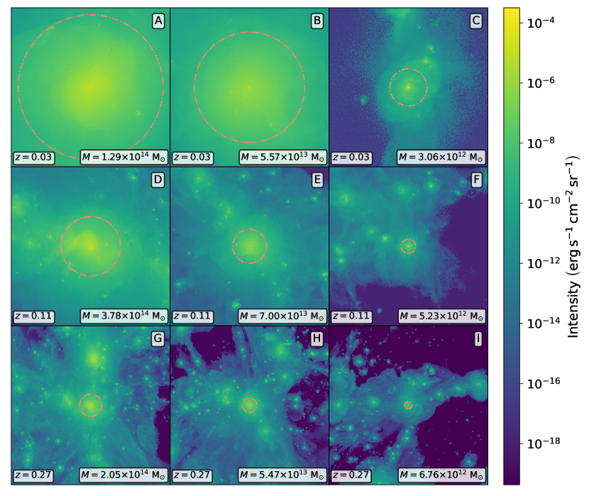
Figure 2: X-ray emissivity maps of the selected targets. Each image is $256\times 256$ in dimension, covering a sky region of $1\degr\times 1\degr$. The dash-dot circle is of radius $r_{200}$. Note that zero-valued pixels were set to the minimum value of a map.

3.3 Light cone

In reality, along the line of sight towards a target, other sources (e.g., star-forming galaxies or clusters) could also produce X-ray emission lines in the energy range of interest. To mimic actual observations, light cones need to be generated and used when creating mock observations. Along a line of sight, only photons from within the corresponding light cone can reach the detector.

In order to generate light cones from the simulated data without repeated structures, we used the method of 2007MNRAS.376….2K . The key to this method is to use a pair of integers $(n,m)$ that have no common denominator. The details of the method can be found in (2007MNRAS.376….2K, , Section 2.4.1). Briefly, the integer pair sets the direction vector of a line of sight as $\mathbf{u_{3}}=\left.\left(n,m,mn\right)\right/\left(n^{2}+m^{2}+m^{2}n^{2}\right)^{\left.1\right/2}$. The light cone along the line of sight would be ensured of no repeating structures from the origin to the positions at coordinates $\left(\left(n\pm\left.0.5\right/m\right)L,\left(m\pm\left.0.5\right/n\right)L,nmL\right)$ in the data cube. The angular area covered by the light cone is about $\left.1\right/\left(m^{2}n\right)\times\left.1\right/\left(n^{2}m\right)~{}\mathrm{\left(rad^{2}\right)}$. In other words, for a chosen pair of integers, the redshift range and angular area of the light cone are uniquely determined.

Considering the size of TNG100 data cubes and the design parameters of the HUBS payload, we chose $(n,m)=(4,3)$ to generate a light cone, corresponding to an angular area of $\sim 1.59\degr\times 1.19\degr$ (which is slightly larger than the FoV of HUBS) and a redshift range of roughly $0\text{--}0.356$. For making mock light-cone observations, we stacked the TNG100 snapshots at $z=0.01$, $0.03$, $0.06$, $0.11$, $0.18$, $0.27$, and $0.35$. Through swapping the integers $(n,m)$, changing the origin (e.g. $(0,0,0)\mapsto(L,0,0)$, where $L$ is the side of the box), and permutating coordinate axes (e.g. $x\mapsto y$, $y\mapsto z$ and $z\mapsto x$), $48$ light cones were generated. For this work, we took the one that contains no extremely bright structures, compared with the selected targets (as shown in Table 3.2).

We used the same light cone to generate mock observations of all targets. Briefly, to produce a mock observation of a target, the light cone was divided into redshift slices. Each slice was treated as an individual observation at one redshift, and all slices are integrated to produce the overall X-ray emission along the light cone. Then, we put the target in the light cone, calculated its X-ray emission, and added it, along with the foreground and background emission (see Sec. 3.4), to the light-cone contribution, producing the final mock observation.

3.4 Foreground and background

Hot gas also exists in our own Galaxy. It is often characterized in terms of the so-called “Local Hot Bubble” and Galactic halo. In addition, the ions in the solar wind can exchange electric charge with neutral atoms in the interstellar medium or in the Earth exosphere, to produce X-ray emission whose spectrum is also dominated by emission lines. Together, they form a foreground for observing an extragalactic source.

For this work, the X-ray foreground was generated with the SOXS (v3.0.2) package. The X-ray spectrum was calculated with the apec code (v3.0.9; 2012ApJ…756..128F ), assuming the hot gas is in collisional ionization equilibrium (which is generally the case for the sources of interest here). We used two apec components to approximate the foreground emission.

The X-ray background mainly originates in unresolved active galactic nuclei (AGN) and, to a lesser extent, normal galaxies. The latter are already included in the light-cone component. To compute the AGN contribution, we used the $\log N-\log S$ relation 2012ApJ…752…46L to create a population of background AGN. Each source was assumed to have an X-ray spectrum of power-law shape, with photon indices drawn from the distribution of measured values (see Fig. 13a of 2006ApJ…645…95H, ). The X-ray spectrum of the AGN background was generated also with the SOXS package.

3.5 Summary of procedures

In summary, the steps for generating mock observations are as follows:

• Selecting a halo of mass appropriate for the target of interest from the TNG100 data, for a given redshift, and placing it at the centre of a sky field of roughly $1\degr\times 1\degr$ in size.

• Computing the X-ray emission using the pyXSIM package, based on the density, temperature, metallicity of each gas element in the target, under the assumption that the X-ray spectrum is described by the apec model. The X-ray photons was then redshifted appropriately, according to the redshift of the target. In this step, we assumed an exposure time of $1~{}\mathrm{Ms}$ and a collecting area of $A_{\text{coll}}=1000~{}\mathrm{cm^{2}}$ for generating X-ray photons.

• Projecting the X-ray photons along the line of sight to the target. Based on the peculiar velocity of each particle, the wavelength of X-ray photons is Doppler-shifted (in addition to the cosmological redshift). To relate to observations, foreground absorption was implemented with the tbabs model 2000ApJ…542..914W , assuming an interstellar hydrogen column density of $N_{\rm{H}}=4\times 10^{20}~{}\mathrm{cm^{-2}}$.

• Making a light cone to account for X-ray emission from sources other than the target along the line of sight. We computed X-ray emission from all objects that lie inside the light cone.

• Generating X-ray foreground and background for the mock observation.

• Convolving the overall X-ray emission (from the target, light cone, AGN background, and Galactic foreground) with the instrument responses (RMF and ARF) using the instrument simulator module in the SOXS package, to generate the detected events.

• Binning the events in spatial and spectral coordinates, respectively, to construct mock X-ray images and spectra.

4 Analyses and Results

4.1 Imaging analyses

Fig. 3 shows the images derived from the mock observations. Much of the large-scale filamentary structures (as seen in the emission maps in Fig. 2) is no longer discernible in the images, but X-ray emissions from CGM, IGrM or ICM of the target source are detected.

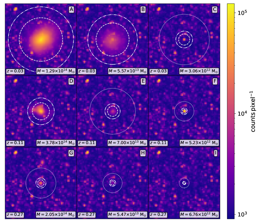
Figure 3: Mock 0.1-2 keV X-ray images of the selected targets, with an assumed exposure time of $1~{}\mathrm{Ms}$. The dashed, dot-dashed and dotted circles are of radii $r_{500}$, $r_{200}$, and $3r_{200}$, respectively. Each image is $60\times 60$ in dimension (with $1\arcmin$/pixel), covering a sky region of $1\degr\times 1\degr$.

To emulate data analyses with real observations, we used the DAOStarFinder tool in the photutils package to detect point-like sources (i.e., the background AGN) in the images. For that, a 2-d Gaussian kernel of radius $1.5$ pixels (FWHM) was employed, with the detection threshold set at $3\sigma$ (above the local background). The detected point-like sources were removed by masking out a circular area of diameter $3$ pixels around each source. The blank pixels were then filled with values interpolated from neighboring pixels using the interpolate_replace_nans script (in astropy).

Then, We proceeded to detect and remove contamination from extended sources (e.g. star-forming galaxies) in the light cone, with the detect_sources tool in the photutils package, with the detection threshold set at $3\sigma$ (and the npixels parameter set to 5). As an example, Fig. 4 shows a cleaned image around a target, where the blank pixels are associated with extended contaminating sources.

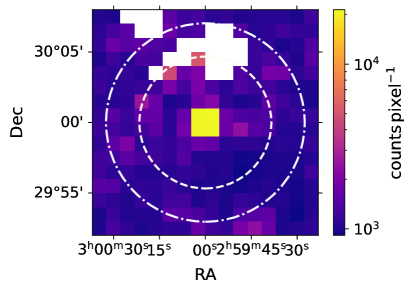
Figure 4: Zoomed-in image of Target C. The blank pixels are associated with the removed sources. The dashed and dot-dashed circles show regions of radius $r_{500}$ and $r_{200}$, respectively.

To improve the signal-to-noise ratio of spatial analyses, we also made images using the same approach as described above but in a narrow band around the bright (red-shifted) O vii and O viii emission lines, respectively. The results are given in Figs. 5 and 6. As can be seen, the extended X-ray emission from CGM stands out more significantly in the narrow-band images (in particular, around O viii); so does that of IGrM (for groups) and ICM (for clusters).

To be more quantitative, we made radial profiles from the images. Examples are shown in Fig. 7 for the cluster, group, and galaxy, respectively, at redshift $z=0.03$. For both the cluster and group, while the narrow-band profile generally follows the full-band profile around the O vii line, roughly to $r_{500}$, it is significantly steeper than the full-band profile around the O viii line and extends beyond $r_{200}$. The increase in the ratio of O vii and O vii surface brightness would be consistent with a cooler outskirt in these systems. The galaxy is a bit difficult to resolve even at such a low redshift, which indicates that the primary targets for CGM studies with HUBS are nearby galaxies. In this case, it can still be seen that the narrow-band profiles are more extended than the full-band profile.

The results indicate that HUBS would be quite effective in detecting emission from hot CGM, through direct imaging, but may be limited to nearby (or low-redshift) galaxies. IGrM and ICM could, on other hand, be well imaged at higher redshifts (beyond $z\sim 0.3$). The results also illustrate the power of a large FoV: even at redshifts as low as 0.03, HUBS would still be able to capture a galaxy cluster in its entirety with one pointing, enabling spatially-resolved spectroscopy.

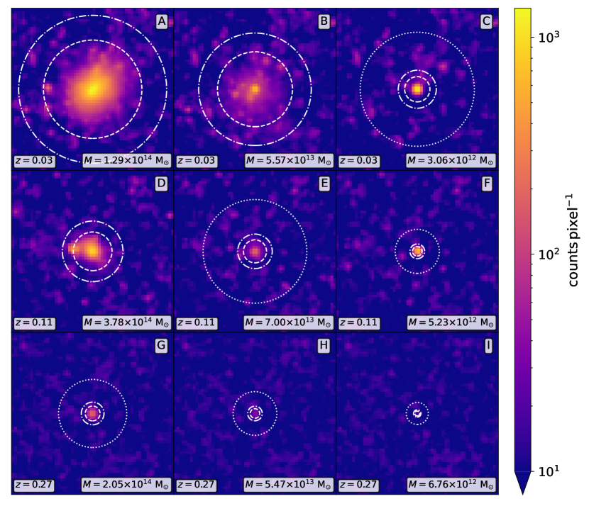
Figure 5: As for Fig. 3, but in a narrow band around the (redshifted) O vii emission line. The width of the band was chosen to be about 18 eV, to ensure the inclusion of the line triplets. The point-like and extended sources detected in the full-band images were removed and the images smoothed.

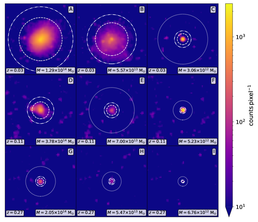
Figure 6: As for Fig. 5, but in a narrow band around the (redshifted) O viii emission line.

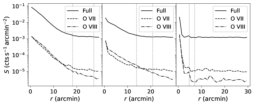
Figure 7: The radial profiles of Target A (left), Target B (middle), and Target C (right), respectively. As indicated, the profiles were derived from the full-band and narrow-band images, and are shown separately. The dotted lines indicate $r_{500}$ and $r_{200}$.

4.2 Spectral analyses

To obtain the X-ray spectrum of a target, we collected all photons from within a circular region of radius $r_{200}$ that is centered at the target. Instead of taking a more traditional approach to background subtraction, we chose to include various contributions (the target, light cone, AGN background and Galactic foreground) in the model for spectral fitting. As an example, Fig. 8 shows the mock spectrum of Target C. The (redshifted) emission lines expected of the CGM are indicated at the top of the figure. We note that the strong emission lines are associated with the foreground, which could make it challenging for HUBS to accurately measure the emission lines associated with an extragalactic source. Fig. 8 also shows zoomed-in views of the mock spectrum around the O vii and O viii lines. Besides the emission lines associated with the target, the presence of the foreground (strongest) lines are apparent, along with weak lines likely associated with star-forming galaxies in the light cone.

Taking the conventionally approach to spectral modeling, we fitted the X-ray spectrum in xspec 1996ASPC..101…17A with a model that consists of following components:

• Three bapec components, approximating the X-ray emission from a multiphase hot gas of the target galaxy;

• Two apec components, accounting for the Galactic foreground;

• One powerlaw component, modeling the AGN background (plus other continuum);

• A number of gauss components, representing the weak emission lines associated with other X-ray sources (e.g. star-forming galaxies) in the light cone.

The interstellar absorption was computed with tbabs (also in xspec), assuming a fixed hydrogen column density of $N_{\rm{H}}=4\times 10^{20}~{}\mathrm{cm^{-2}}$. Compared with the apec model, the bapec model considers the effects of velocity broadening, which is more appropriate for the targets of interest here. In order to make use of the full spectral resolution in the fitting, we adopted C-statistics 1979ApJ…228..939C to provide an unbiased estimate of the model parameters 2009ApJ…693..822H , allowing low counts ($<10$) in some of the spectral bins. The spectral fitting was carried out over an energy range of $0.1\text{--}2~{}\mathrm{keV}$. Other than $N_{\rm{H}}$ and the parameters of the foreground, all other parameters in the model were allowed to vary. An example of the best-fitting model is shown in Fig. 8.

Table 2 shows the key parameters that characterize the properties of the emitting gas (including temperature, metalicity, redshift, and velocity dispersion). Covariance analysis was carried out to assess correlations among the model paramters and to derive confidence intervals of the parameters. We found a significant correlation between the normalization and metalicity in each bapec component, but none between other parameter pairs.

Similar spectral analyses were also carried out for galaxy groups and clusters in the target sample, to measure the properties of IGrM and ICM. The results are also summarized in Table 2. As examples, Figs. 9 and  10 show the overall X-ray spectra of Target E and Target D, respectively. Zoomed-in views are shown in the figures, focusing on the regions around the O vii and O viii lines. Again, in both cases, deviations from the best-fitting models perhaps indicate possible contribution from contaminating sources in the light cone but, more importantly, inaccuracy in modeling X-ray emission from the hot gas with several discrete bapec components (see discussion below).

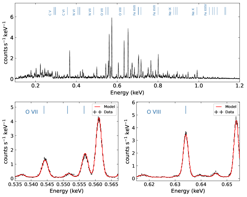
Figure 8: Top panel: Mock X-ray spectrum of Target C. It was made with X-ray photons within a circular region of radius $r_{200}$ centred at the target. At the top, some of the strong emission lines associated with the target are indicated. Bottom panel: Zoomed-in view of the top panel, around the O vii line triplets (left), and the O viii K$\alpha$ line (right). Also shown is the best-fitting model (in solid line). The strongest lines are due to the foreground. Some of the weak lines are associated with the light-cone component.

Table 2: Results of spectral fitting for the targets

Component	Parameter	Unit	Target C	Target E	Target D
bapec-1	$kT$	$\mathrm{keV}$	$0.426_{-0.005}^{+0.005}$	$0.712_{-0.007}^{+0.005}$	$2.26_{-0.04}^{+0.02}$
bapec-1	$Z$	$\mathrm{Z_{\sun}}$	$0.59_{-0.03}^{+0.06}$	$0.066_{-0.002}^{+0.005}$	$0.339_{-0.008}^{+0.009}$
bapec-1	redshift		$0.03054_{-0.00001}^{+0.00002}$	$0.11030_{-0.00005}^{+0.00003}$	$0.10944_{-0.00001}^{+0.00001}$
bapec-1	$\sigma_{\mathrm{v}}$	$\mathrm{km\,s^{-1}}$	$192_{-10}^{+5}$	$274_{-14}^{+18}$	$242_{-3}^{+5}$
bapec-1	norma	$\mathrm{cm^{-5}}$	$9.8_{-1.0}^{+0.5}\times 10^{-5}$	$6.4_{-0.3}^{+0.1}\times 10^{-4}$	$5.63_{-0.07}^{+0.13}\times 10^{-3}$
bapec-2	$kT$	$\mathrm{keV}$	$0.197_{-0.001}^{+0.003}$	$0.250_{-0.008}^{+0.005}$	$0.659_{-0.010}^{+0.008}$
bapec-2	$Z$	$\mathrm{Z_{\sun}}$	$0.52_{-0.04}^{+0.04}$	$0.40_{-0.04}^{+0.05}$	$0.034_{-0.002}^{+0.002}$
bapec-2	redshift		$0.03078_{-0.00002}^{+0.00002}$	$0.11003_{-0.00010}^{+0.00014}$	$0.10955_{-0.00005}^{+0.00008}$
bapec-2	$\sigma_{\mathrm{v}}$	$\mathrm{km\,s^{-1}}$	$170_{-14}^{+15}$	$247_{-27}^{+41}$	$512_{-17}^{+25}$
bapec-2	norm	$\mathrm{cm^{-5}}$	$1.14_{-0.08}^{+0.10}\times 10^{-4}$	$3.3_{-0.4}^{+0.4}\times 10^{-5}$	$1.88_{-0.12}^{+0.07}\times 10^{-3}$
bapec-3	$kT$	$\mathrm{keV}$	$0.871_{-0.008}^{+0.006}$	$1.31_{-0.01}^{+0.01}$	$1.205_{-0.018}^{+0.009}$
bapec-3	$Z$	$\mathrm{Z_{\sun}}$	$0.107_{-0.006}^{+0.009}$	$0.49_{-0.03}^{+0.06}$	$2.2_{-0.2}^{+0.2}$
bapec-3	redshift		$0.03066_{-0.00002}^{+0.00005}$	$0.11047_{-0.00004}^{+0.00004}$	$0.10933_{-0.00003}^{+0.00003}$
bapec-3	$\sigma_{\mathrm{v}}$	$\mathrm{km\,s^{-1}}$	$127_{-14}^{+14}$	$143_{-12}^{+16}$	$265_{-11}^{+8}$
bapec-3	norm	$\mathrm{cm^{-5}}$	$2.6_{-0.2}^{+0.2}\times 10^{-4}$	$1.5_{-0.1}^{+0.1}\times 10^{-4}$	$1.50_{-0.17}^{+0.08}\times 10^{-4}$

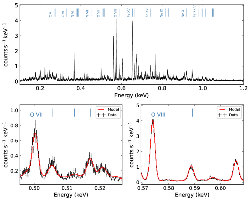
Figure 9: As for Fig. 8, but for Target E.

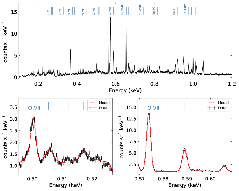
Figure 10: As for Fig. 8, but for Target D. Note the presence of more emission lines associated with the light-cone component, around the O viii line.

5 Discussion

Through analyzing mock observations, it has become fairly clear that, even for a highly-optimized X-ray mission like HUBS, it would likely require careful selection of targets and large investment in observing resources to obtain data of decent quality for studying the hot phase of CGM systematically, due primarily to the weakness of the expected signals, and also to the presence of strong foreground emission (and possibly contamination by other sources in the FoV). What has not been addressed in this work is the problem of separating X-ray emission from the hot CGM and interstellar medium in a target galaxy, owing to the limited angular resolution of HUBS. Some of these challenges could be mitigated also through target selection, making use of a wealth of multiwavelength information obtained from prior observations.

Observationally, spectral analysis with HUBS data is expected to be quite challenging, due again to the presence of (in some cases) overwhelming foreground lines. Avoiding those lines would also impose constraints on the redshifts. Blending of target lines with foreground lines would complicate reliable modeling. For targets not filling the entire FoV, the standard approach of background subtraction may be effective, although systematic uncertainties could be an issue. At a more fundamental level, it is challenging to model gas with a continuous temperature distribution rigorously in practice; instead, as described in Section 4.2, it is often approximated with a few discrete components, each of which is characterized by a temperature. The question is how well such an approach can recover the primary phases of the gas. Vijayan & Li 2021arXiv210211510V described modeling with a log-normal distribution in temperature, which seems to provide more reliable results. Novel techniques like this would be required for analyzing X-ray spectra of high resolution in the future.

5.1 Determining the properties of hot gas

The properties of the hot gas associated with the selected targets have been obtained through spectral analyses. The results can be compared with the properties in the input (simulation). Specifically, we examine how well the spectral analyses could capture the principal phases of the emitting gas.

Fig. 11 shows the theoretical distributions of temperature and abundances (from the TNG data) for Targets C, E and D , respectively. These were calculated using all gas particles within the chosen spherical region of radius $r_{200}$ for each halo. Also shown in the figure are the temperature and abundances derived from the spectral modeling. They capture the main components of the multi-phase gas fairly well, but traditional spectral modeling with discrete components clearly shows its limits, partly due to the relatively narrow energy range that HUBS is designed to cover. As the figure shows, the approach works very well for the group (Target E), but only marginally for the galaxy (Target C), because the temperature of its CGM is generally quite low and the associated X-ray emission is thus too soft (and weak) even for HUBS. At the opposite end, the ICM in the cluster (Target D) seems a bit too hot (thus the associated X-ray emission too hard) for HUBS observations to constrain its properties as well as the group.

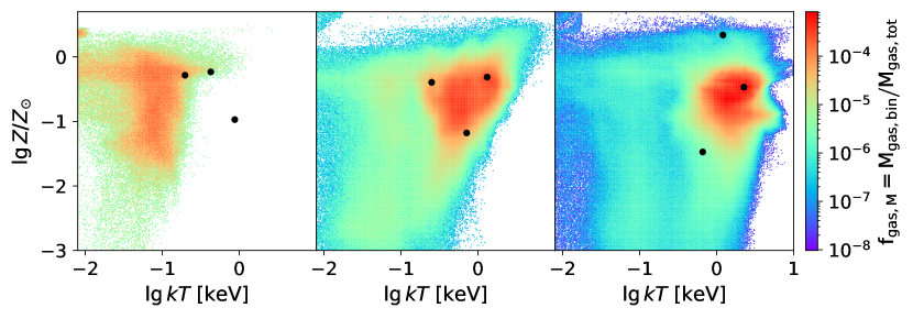
Figure 11: Theoretical phase diagrams ($Z-kT$) for Target C, E and D, respectively. The data were derived from the TNG simulation. For comparison, the results from spectral analyses are shown in black dots.

5.2 Detection limits

Of general interest is the sensitivity of HUBS to low surface brightness X-ray emission. With the contributions from the light cone, foreground and background components quantified, we can now assess the sensitivity to some of the emission lines of interest (see Fig. 8) fairly realistically. Due to the presence of contaminating lines (associated mainly with the foreground but also with star-forming galaxies along the line of sight), the results derived here are necessarily redshift dependent. We chose $z=0.03$ for deriving surface brightness limits.

We added X-ray events that are associated with the light cone, Galactic foreground, and AGN background to generate an overall X-ray spectrum, and fitted it with the same model as before (see Section 4.2). We then added to the best-fitting model a Gaussian component (zgauss in xspec), to represent an emission line of interest. We fixed the line energy at the intended (redshifted) value and the line width at $\sigma_{K}=0.1~{}\mathrm{eV}$ (accounting for Doppler broadening), and only allowed the normalization of the Gaussian component to vary. We also froze all other model parameters, and fitted the spectrum again, based on C-statistics. The normalization (of zgauss) was varied until $\Delta C$ provides a $5\sigma$ upper limit. The limiting line surface brightness was then computed. Repeating the procedure, we obtained results for other emission lines of interest. The results are summarized in Table 3.

For comparison, we note that the limiting sensitivity of Athena for O vii (r) is about $0.12~{}\mathrm{photons\,s^{-1}\,cm^{-2}\,sr^{-1}}$ for $10^{6}~{}\mathrm{arcmin^{2}\,s}$ (without considering lightcone contribution) 2021arXiv210804847W .

Some caveats should be noted. At low X-ray energies, the Galactic foreground is known to be patchy, so the limiting surface brightness is expected to vary significantly among different lines of sight. In addition, throughout this work, we ignored the detector background due to charged particles in orbit, because it is expected to be negligible.

Table 3: Line surface brightness limits^†

Line	Rest-frame energy	Surface brightness limit
	$\left(\mathrm{eV}\right)$	$\left(\mathrm{photons\,s^{-1}\,cm^{-2}\,sr^{-1}}\right)$
N vii	$500$	$1.1\times 10^{-3}$
O viii	$654$	$2.1\times 10^{-3}$
O vii (r)	$574$	$3.2\times 10^{-3}$
Fe xvii	$826$	$2.4\times 10^{-3}$
Ne x	$1022$	$1.2\times 10^{-3}$

^† Derived for 5-$\sigma$ detection with an exposure time of 1 Ms.

6 Summary

We created mock observations for HUBS, based on the IllustrisTNG-100 simulation, and used them to assess the scientific capabilities of HUBS in detecting extended X-ray emission from the hot gas in galaxies, groups, and clusters at different redshifts. As expected, the X-ray emission from relatively dense environments (CGM, IGrM, and ICM) can be detected efficiently, at low redshifts, thanks in part to the large FoV of HUBS. On the other hand, the emission from filamentary structures in the IGM would seem too faint to be seen (comparing Figs. 2 and 3). Useful insights into IGM could be gained through studying the outskirt of clusters (perhaps also superclusters).

For a 2-eV energy resolution of the detector, the emission lines from sources at redshifts lower than about $z=0.01$ become inseparable from those of the foreground emission, although they can still be studied by measuring the foreground and background (and line-of-sight) contribution from the images, as long as they do not fill the entire FoV. The upper redshift bound is determined by the detection sensitivity of HUBS, as well as by the brightness of the target. Our results show that it lies around $z\sim 0.2$ for galaxies (see Fig. 6), and beyond $z\sim 0.3$ for groups and clusters. Therefore, HUBS is mainly for observing targets at relatively low redshifts. It is worth noting that HUBS would be well suited for measuring hot IGrM around galaxy groups, and the cooler outskirts of ICM and perhaps also IGM in the cluster environment, with its large FoV. Even at the centre of ICM, HUBS would be quite effective in probing the relatively cooler phase of the gas.

The main conclusions of this work are summarised as follows.

1. A dedicated X-ray spectroscopic mission similar to HUBS would be required to enable significant progress in measuring the spatial distribution and properties of the CGM around nearby galaxies.

2. Galaxy groups would be excellent targets for HUBS, as the hot phase of IGrM peaks around temperatures $kT\sim 1~{}\mathrm{keV}$.

3. With its large FoV, HUBS would be quite efficient for spectral studies of clusters, especially the outskirts of ICM, even at fairly low redshifts.

4. At the low end of the accessible redshift range, the Galactic foreground imposes a constraint on the detection of emission lines from an extragalactic source. For a target at a redshift of less than 0.01, its emission lines would be inseparable from the foreground lines, although the traditional background-subtraction method can be applied to the images of sources at even lower redshifts.

5. With 1 Ms exposure time, CGM around galaxies could be detected with HUBS up to a redshift of about 0.2, IGrM around galaxy groups of to about 0.3, and ICM around galaxy clusters further.

6. Even with currently available plasma diagnostic tools, HUBS data can be used to derive the properties of the primary phases of X-ray-emitting hot gas. More advanced tools would be required to study the multiphase gas more realistically.

In this work, we did not consider absorption-line diagnostics. In the payload design of HUBS, though, special consideration has been made to optimize such capability, although the details are still being discussed and may evolve.

Acknowledgements

We thank Dan McCammon for providing the XQC filter data and for useful discussions, and Zhansan Wang for providing preliminary data on the HUBS optics. We would also like to thank John ZuHone for useful suggestion on using some of the software packages, and Taotao Fang for advice on making mock observations. This work was supported in part by the Ministry of Science and Technology of China through its National Key R&D Program, Grant 2018YFA0404502, and by the National Natural Science Foundation of China through Grant 11821303. This work made use of several Python packages for astronomy, including pyXSIM 2014arXiv1407.1783Z ; 2016ascl.soft08002Z , photutils 2020zndo…4049061B , astropy 2013A&A…558A..33A ; 2018AJ….156..123A . The figures in this paper were made using the python matplotlib 2007CSE…..9…90H and seaborn 2018zndo…1313201W package.

Declarations

Funding

This work was supported in part by the Ministry of Science and Technology of China through its National Key R&D Program, Grant 2018YFA0404502, and by the National Natural Science Foundation of China through Grant 11821303.

Data Availability

The IllustrisTNG halo catalogues and the simulation snapshots 2019ComAC…6….2N are publicly available at http://www.tng-project.org/data/. The rest of the data underlying the article will be available from the corresponding author on reasonable request.

References

- \bibcommenthead
- (1) Tumlinson, J., Peeples, M.S., Werk, J.K.: The Circumgalactic Medium. ARA&A 55(1), 389–432 (2017) arXiv:1709.09180 [astro-ph.GA]. https://doi.org/10.1146/annurev-astro-091916-055240
- (2) Wang, Q.D., Immler, S., Walterbos, R., Lauroesch, J.T., Breitschwerdt, D.: Chandra Detection of a Hot Gaseous Corona around the Edge-on Galaxy NGC 4631. ApJ 555(2), 99–102 (2001) arXiv:astro-ph/0105541 [astro-ph]. https://doi.org/10.1086/323179
- (3) Strickland, D.K., Heckman, T.M., Colbert, E.J.M., Hoopes, C.G., Weaver, K.A.: A High Spatial Resolution X-Ray and H Study of Hot Gas in the Halos of Star-forming Disk Galaxies. I. Spatial and Spectral Properties of the Diffuse X-Ray Emission. ApJS 151(2), 193–236 (2004) arXiv:astro-ph/0306592 [astro-ph]. https://doi.org/%****␣Manuscript.bbl␣Line␣100␣****10.1086/382214
- (4) Tüllmann, R., Pietsch, W., Rossa, J., Breitschwerdt, D., Dettmar, R.-J.: The multi-phase gaseous halos of star forming late-type galaxies. I. XMM-Newton observations of the hot ionized medium. A&A 448(1), 43–75 (2006) arXiv:astro-ph/0510079 [astro-ph]. https://doi.org/10.1051/0004-6361:20052936
- (5) Li, J.-T., Wang, Q.D.: Chandra survey of nearby highly inclined disc galaxies - II. Correlation analysis of galactic coronal properties. MNRAS 435(4), 3071–3084 (2013) arXiv:1308.1933 [astro-ph.CO]. https://doi.org/10.1093/mnras/stt1501
- (6) Li, J.-T., Bregman, J.N., Wang, Q.D., Crain, R.A., Anderson, M.E., Zhang, S.: The Circum-Galactic Medium of Massive Spirals. II. Probing the Nature of Hot Gaseous Halo around the Most Massive Isolated Spiral Galaxies. ApJS 233(2), 20 (2017) arXiv:1710.07355 [astro-ph.GA]. https://doi.org/10.3847/1538-4365/aa96fc
- (7) Anderson, M.E., Bregman, J.N.: Detection of a Hot Gaseous Halo around the Giant Spiral Galaxy NGC 1961. ApJ 737(1), 22 (2011) arXiv:1105.4614 [astro-ph.CO]. https://doi.org/%****␣Manuscript.bbl␣Line␣175␣****10.1088/0004-637X/737/1/22
- (8) Dai, X., Anderson, M.E., Bregman, J.N., Miller, J.M.: XMM-Newton Detects a Hot Gaseous Halo in the Fastest Rotating Spiral Galaxy UGC 12591. ApJ 755(2), 107 (2012) arXiv:1112.0324 [astro-ph.CO]. https://doi.org/10.1088/0004-637X/755/2/107
- (9) Bogdán, Á., Bourdin, H., Forman, W.R., Kraft, R.P., Vogelsberger, M., Hernquist, L., Springel, V.: Probing the Hot X-Ray Corona around the Massive Spiral Galaxy, NGC 6753, Using Deep XMM-Newton Observations. ApJ 850(1), 98 (2017) arXiv:1710.07286 [astro-ph.GA]. https://doi.org/10.3847/1538-4357/aa9523
- (10) Cui, W., Chen, L.-B., Gao, B., Guo, F.-L., Jin, H., Wang, G.-L., Wang, L., Wang, J.-J., Wang, W., Wang, Z.-S., Wang, Z., Yuan, F., Zhang, W.: HUBS: Hot Universe Baryon Surveyor. Journal of Low Temperature Physics 199(1-2), 502–509 (2020). https://doi.org/10.1007/s10909-019-02279-3
- (11) Cui, W., Bregman, J.N., Bruijn, M.P., Chen, L.-B., Chen, Y., Cui, C., Fang, T.-T., Gao, B., Gao, H., Gao, J.-R., Gottardi, L., Gu, K.-X., Guo, F.-L., Guo, J., He, C.-L., He, P.-F., den Herder, J.-W., Huang, Q.-S., Li, F.-J., Li, J.-T., Li, J.-J., Li, L.-Y., Li, T.-P., Li, W.-B., Liang, J.-T., Liang, Y.-J., Liang, G.-Y., Liu, Y.-J., Liu, Z., Liu, Z.-Y., Jaeckel, F., Ji, L., Ji, W., Jin, H., Kang, X., Ma, Y.-X., McCammon, D., Mo, H.-J., Nagayoshi, K., Nelms, K., Qi, R., Quan, J., Ridder, M.L., Shen, Z.-X., Simionescu, A., Taralli, E., Wang, Q.D., Wang, G.-L., Wang, J.-J., Wang, K., Wang, L., Wang, S.-F., Wang, S.-J., Wang, T.-G., Wang, W., Wang, X.-Q., Wang, Y.-L., Wang, Y.-R., Wang, Z., Wang, Z.-S., Wen, N.-Y., de Wit, M., Wu, S.-F., Xu, D., Xu, D.-D., Xu, H.-G., Xu, X.-J., Xu, R.-X., Xue, Y.-Q., Yi, S.-Z., Yu, J., Yang, L.-W., Yuan, F., Zhang, S., Zhang, W., Zhang, Z., Zhong, Q., Zhou, Y., Zhu, W.-X.: HUBS: a dedicated hot circumgalactic medium explorer. In: Society of Photo-Optical Instrumentation Engineers (SPIE) Conference Series. Society of Photo-Optical Instrumentation Engineers (SPIE) Conference Series, vol. 11444, p. 114442 (2020). https://doi.org/10.1117/12.2560871
- (12) McCammon, D., Almy, R., Apodaca, E., Bergmann Tiest, W., Cui, W., Deiker, S., Galeazzi, M., Juda, M., Lesser, A., Mihara, T., Morgenthaler, J.P., Sanders, W.T., Zhang, J., Figueroa-Feliciano, E., Kelley, R.L., Moseley, S.H., Mushotzky, R.F., Porter, F.S., Stahle, C.K., Szymkowiak, A.E.: A High Spectral Resolution Observation of the Soft X-Ray Diffuse Background with Thermal Detectors. ApJ 576(1), 188–203 (2002) arXiv:astro-ph/0205012 [astro-ph]. https://doi.org/10.1086/341727
- (13) Yoshikawa, K., Yamasaki, N.Y., Suto, Y., Ohashi, T., Mitsuda, K., Tawara, Y., Furuzawa, A.: Detectability of the Warm/Hot Intergalactic Medium through Emission Lines of O VII and O VIII. PASJ 55, 879–890 (2003) astro-ph/0303281. https://doi.org/10.1093/pasj/55.5.879
- (14) Fang, T., Croft, R.A.C., Sanders, W.T., Houck, J., Davé, R., Katz, N., Weinberg, D.H., Hernquist, L.: Simulation of Soft X-Ray Emission Lines from the Missing Baryons. ApJ 623, 612–626 (2005) astro-ph/0311141. https://doi.org/10.1086/428656
- (15) Roncarelli, M., Cappelluti, N., Borgani, S., Branchini, E., Moscardini, L.: The effect of feedback on the emission properties of the warm-hot intergalactic medium. MNRAS 424(2), 1012–1025 (2012) arXiv:1202.4275 [astro-ph.CO]. https://doi.org/10.1111/j.1365-2966.2012.21277.x
- (16) Oppenheimer, B.D., Bogdán, Á., Crain, R.A., ZuHone, J.A., Forman, W.R., Schaye, J., Wijers, N.A., Davies, J.J., Jones, C., Kraft, R.P., Ghirardini, V.: EAGLE and Illustris-TNG Predictions for Resolved eROSITA X-Ray Observations of the Circumgalactic Medium around Normal Galaxies. ApJ 893(1), 24 (2020) arXiv:2003.13889 [astro-ph.GA]. https://doi.org/10.3847/2041-8213/ab846f
- (17) Marinacci, F., Vogelsberger, M., Pakmor, R., Torrey, P., Springel, V., Hernquist, L., Nelson, D., Weinberger, R., Pillepich, A., Naiman, J., Genel, S.: First results from the IllustrisTNG simulations: radio haloes and magnetic fields. MNRAS 480, 5113–5139 (2018) arXiv:1707.03396. https://doi.org/10.1093/mnras/sty2206
- (18) Naiman, J.P., Pillepich, A., Springel, V., Ramirez-Ruiz, E., Torrey, P., Vogelsberger, M., Pakmor, R., Nelson, D., Marinacci, F., Hernquist, L., Weinberger, R., Genel, S.: First results from the IllustrisTNG simulations: a tale of two elements - chemical evolution of magnesium and europium. MNRAS 477, 1206–1224 (2018) arXiv:1707.03401. https://doi.org/10.1093/mnras/sty618
- (19) Nelson, D., Pillepich, A., Springel, V., Weinberger, R., Hernquist, L., Pakmor, R., Genel, S., Torrey, P., Vogelsberger, M., Kauffmann, G., Marinacci, F., Naiman, J.: First results from the IllustrisTNG simulations: the galaxy colour bimodality. MNRAS 475, 624–647 (2018) arXiv:1707.03395. https://doi.org/10.1093/mnras/stx3040
- (20) Nelson, D., Springel, V., Pillepich, A., Rodriguez-Gomez, V., Torrey, P., Genel, S., Vogelsberger, M., Pakmor, R., Marinacci, F., Weinberger, R., Kelley, L., Lovell, M., Diemer, B., Hernquist, L.: The IllustrisTNG simulations: public data release. Computational Astrophysics and Cosmology 6, 2 (2019) arXiv:1812.05609. https://doi.org/10.1186/s40668-019-0028-x
- (21) Pillepich, A., Nelson, D., Hernquist, L., Springel, V., Pakmor, R., Torrey, P., Weinberger, R., Genel, S., Naiman, J.P., Marinacci, F., Vogelsberger, M.: First results from the IllustrisTNG simulations: the stellar mass content of groups and clusters of galaxies. MNRAS 475(1), 648–675 (2018) arXiv:1707.03406 [astro-ph.GA]. https://doi.org/10.1093/mnras/stx3112
- (22) Springel, V., Pakmor, R., Pillepich, A., Weinberger, R., Nelson, D., Hernquist, L., Vogelsberger, M., Genel, S., Torrey, P., Marinacci, F., Naiman, J.: First results from the IllustrisTNG simulations: matter and galaxy clustering. MNRAS 475, 676–698 (2018) arXiv:1707.03397. https://doi.org/10.1093/mnras/stx3304
- (23) Springel, V.: E pur si muove: Galilean-invariant cosmological hydrodynamical simulations on a moving mesh. MNRAS 401, 791–851 (2010) arXiv:0901.4107. https://doi.org/10.1111/j.1365-2966.2009.15715.x
- (24) Springel, V., White, S.D.M., Tormen, G., Kauffmann, G.: Populating a cluster of galaxies - I. Results at [formmu2]z=0. MNRAS 328, 726–750 (2001) astro-ph/0012055. https://doi.org/10.1046/j.1365-8711.2001.04912.x
- (25) Dolag, K., Borgani, S., Murante, G., Springel, V.: Substructures in hydrodynamical cluster simulations. MNRAS 399, 497–514 (2009) arXiv:0808.3401. https://doi.org/10.1111/j.1365-2966.2009.15034.x
- (26) Planck Collaboration, Ade, P.A.R., Aghanim, N., Arnaud, M., Ashdown, M., Aumont, J., Baccigalupi, C., Banday, A.J., Barreiro, R.B., Bartlett, J.G., Bartolo, N., Battaner, E., Battye, R., Benabed, K., Benoît, A., Benoit-Lévy, A., Bernard, J.-P., Bersanelli, M., Bielewicz, P., Bock, J.J., Bonaldi, A., Bonavera, L., Bond, J.R., Borrill, J., Bouchet, F.R., Boulanger, F., Bucher, M., Burigana, C., Butler, R.C., Calabrese, E., Cardoso, J.-F., Catalano, A., Challinor, A., Chamballu, A., Chary, R.-R., Chiang, H.C., Chluba, J., Christensen, P.R., Church, S., Clements, D.L., Colombi, S., Colombo, L.P.L., Combet, C., Coulais, A., Crill, B.P., Curto, A., Cuttaia, F., Danese, L., Davies, R.D., Davis, R.J., de Bernardis, P., de Rosa, A., de Zotti, G., Delabrouille, J., Désert, F.-X., Di Valentino, E., Dickinson, C., Diego, J.M., Dolag, K., Dole, H., Donzelli, S., Doré, O., Douspis, M., Ducout, A., Dunkley, J., Dupac, X., Efstathiou, G., Elsner, F., Enßlin, T.A., Eriksen, H.K., Farhang, M., Fergusson, J., Finelli, F., Forni, O., Frailis, M., Fraisse, A.A., Franceschi, E., Frejsel, A., Galeotta, S., Galli, S., Ganga, K., Gauthier, C., Gerbino, M., Ghosh, T., Giard, M., Giraud-Héraud, Y., Giusarma, E., Gjerløw, E., González-Nuevo, J., Górski, K.M., Gratton, S., Gregorio, A., Gruppuso, A., Gudmundsson, J.E., Hamann, J., Hansen, F.K., Hanson, D., Harrison, D.L., Helou, G., Henrot-Versillé, S., Hernández-Monteagudo, C., Herranz, D., Hildebrand t, S.R., Hivon, E., Hobson, M., Holmes, W.A., Hornstrup, A., Hovest, W., Huang, Z., Huffenberger, K.M., Hurier, G., Jaffe, A.H., Jaffe, T.R., Jones, W.C., Juvela, M., Keihänen, E., Keskitalo, R., Kisner, T.S., Kneissl, R., Knoche, J., Knox, L., Kunz, M., Kurki-Suonio, H., Lagache, G., Lähteenmäki, A., Lamarre, J.-M., Lasenby, A., Lattanzi, M., Lawrence, C.R., Leahy, J.P., Leonardi, R., Lesgourgues, J., Levrier, F., Lewis, A., Liguori, M., Lilje, P.B., Linden-Vørnle, M., López-Caniego, M., Lubin, P.M., Macías-Pérez, J.F., Maggio, G., Maino, D., Mandolesi, N., Mangilli, A., Marchini, A., Maris, M., Martin, P.G., Martinelli, M., Martínez-González, E., Masi, S., Matarrese, S., McGehee, P., Meinhold, P.R., Melchiorri, A., Melin, J.-B., Mendes, L., Mennella, A., Migliaccio, M., Millea, M., Mitra, S., Miville-Deschênes, M.-A., Moneti, A., Montier, L., Morgante, G., Mortlock, D., Moss, A., Munshi, D., Murphy, J.A., Naselsky, P., Nati, F., Natoli, P., Netterfield, C.B., Nørgaard-Nielsen, H.U., Noviello, F., Novikov, D., Novikov, I., Oxborrow, C.A., Paci, F., Pagano, L., Pajot, F., Paladini, R., Paoletti, D., Partridge, B., Pasian, F., Patanchon, G., Pearson, T.J., Perdereau, O., Perotto, L., Perrotta, F., Pettorino, V., Piacentini, F., Piat, M., Pierpaoli, E., Pietrobon, D., Plaszczynski, S., Pointecouteau, E., Polenta, G., Popa, L., Pratt, G.W., Prézeau, G., Prunet, S., Puget, J.-L., Rachen, J.P., Reach, W.T., Rebolo, R., Reinecke, M., Remazeilles, M., Renault, C., Renzi, A., Ristorcelli, I., Rocha, G., Rosset, C., Rossetti, M., Roudier, G., Rouillé d’Orfeuil, B., Rowan-Robinson, M., Rubiño-Martín, J.A., Rusholme, B., Said, N., Salvatelli, V., Salvati, L., Sandri, M., Santos, D., Savelainen, M., Savini, G., Scott, D., Seiffert, M.D., Serra, P., Shellard, E.P.S., Spencer, L.D., Spinelli, M., Stolyarov, V., Stompor, R., Sudiwala, R., Sunyaev, R., Sutton, D., Suur-Uski, A.-S., Sygnet, J.-F., Tauber, J.A., Terenzi, L., Toffolatti, L., Tomasi, M., Tristram, M., Trombetti, T., Tucci, M., Tuovinen, J., Türler, M., Umana, G., Valenziano, L., Valiviita, J., Van Tent, F., Vielva, P., Villa, F., Wade, L.A., Wandelt, B.D., Wehus, I.K., White, M., White, S.D.M., Wilkinson, A., Yvon, D., Zacchei, A., Zonca, A.: Planck 2015 results. XIII. Cosmological parameters. A&A 594, 13 (2016) arXiv:1502.01589 [astro-ph.CO]. https://doi.org/10.1051/0004-6361/201525830
- (27) Davis, M., Efstathiou, G., Frenk, C.S., White, S.D.M.: The evolution of large-scale structure in a universe dominated by cold dark matter. ApJ 292, 371–394 (1985). https://doi.org/10.1086/163168
- (28) Simionescu, A., Allen, S.W., Mantz, A., Werner, N., Takei, Y., Morris, R.G., Fabian, A.C., Sanders, J.S., Nulsen, P.E.J., George, M.R., Taylor, G.B.: Baryons at the Edge of the X-ray-Brightest Galaxy Cluster. Science 331(6024), 1576 (2011) arXiv:1102.2429 [astro-ph.CO]. https://doi.org/10.1126/science.1200331
- (29) Gastaldello, F., Simionescu, A., Mernier, F., Biffi, V., Gaspari, M., Sato, K., Matsushita, K.: The Metal Content of the Hot Atmospheres of Galaxy Groups. Universe 7(7), 208 (2021) arXiv:2106.13258 [astro-ph.CO]. https://doi.org/10.3390/universe7070208
- (30) Kitzbichler, M.G., White, S.D.M.: The high-redshift galaxy population in hierarchical galaxy formation models. MNRAS 376(1), 2–12 (2007) arXiv:astro-ph/0609636 [astro-ph]. https://doi.org/10.1111/j.1365-2966.2007.11458.x
- (31) Foster, A.R., Ji, L., Smith, R.K., Brickhouse, N.S.: Updated Atomic Data and Calculations for X-Ray Spectroscopy. ApJ 756, 128 (2012) arXiv:1207.0576 [astro-ph.HE]. https://doi.org/10.1088/0004-637X/756/2/128
- (32) Lehmer, B.D., Xue, Y.Q., Brandt, W.N., Alexander, D.M., Bauer, F.E., Brusa, M., Comastri, A., Gilli, R., Hornschemeier, A.E., Luo, B., Paolillo, M., Ptak, A., Shemmer, O., Schneider, D.P., Tozzi, P., Vignali, C.: The 4 Ms Chandra Deep Field-South Number Counts Apportioned by Source Class: Pervasive Active Galactic Nuclei and the Ascent of Normal Galaxies. ApJ 752, 46 (2012) arXiv:1204.1977. https://doi.org/10.1088/0004-637X/752/1/46
- (33) Hickox, R.C., Markevitch, M.: Absolute Measurement of the Unresolved Cosmic X-Ray Background in the 0.5-8 keV Band with Chandra. ApJ 645, 95–114 (2006) astro-ph/0512542. https://doi.org/10.1086/504070
- (34) Wilms, J., Allen, A., McCray, R.: On the Absorption of X-Rays in the Interstellar Medium. ApJ 542, 914–924 (2000) astro-ph/0008425. https://doi.org/10.1086/317016
- (35) Arnaud, K.A.: In: Jacoby, G.H., Barnes, J. (eds.) XSPEC: The First Ten Years. Astronomical Society of the Pacific Conference Series, vol. 101, p. 17 (1996)
- (36) Cash, W.: Parameter estimation in astronomy through application of the likelihood ratio. ApJ 228, 939–947 (1979). https://doi.org/10.1086/156922
- (37) Humphrey, P.J., Liu, W., Buote, D.A.: 2 and Poissonian Data: Biases Even in the High-Count Regime and How to Avoid Them. ApJ 693(1), 822–829 (2009) arXiv:0811.2796 [astro-ph]. https://doi.org/10.1088/0004-637X/693/1/822
- (38) Vijayan, A., Li, M.: X-ray Spectra of Circumgalactic Medium Around Star-Forming Galaxies: Connecting Simulations to Observations. arXiv e-prints, 2102–11510 (2021) arXiv:2102.11510 [astro-ph.GA]
- (39) Wijers, N.A., Schaye, J.: The warm-hot circumgalactic medium around EAGLE-simulation galaxies and its detection prospects with X-ray line emission. arXiv e-prints, 2108–04847 (2021) arXiv:2108.04847 [astro-ph.GA]
- (40) ZuHone, J.A., Biffi, V., Hallman, E.J., Randall, S.W., Foster, A.R., Schmid, C.: Simulating X-ray Observations with Python. arXiv e-prints (2014) arXiv:1407.1783 [astro-ph.IM]
- (41) ZuHone, J.A., Hallman, E.J.: pyXSIM: Synthetic X-ray observations generator. Astrophysics Source Code Library (2016)
- (42) Bradley, L., Sipőcz, B., Robitaille, T., Tollerud, E., Vinícius, Z., Deil, C., Barbary, K., Wilson, T.J., Busko, I., Günther, H.M., Cara, M., Conseil, S., Bostroem, A., Droettboom, M., Bray, E.M., Andersen Bratholm, L., Lim, P.L., Barentsen, G., Craig, M., Pascual, S., Perren, G., Greco, J., Donath, A., De Val-Borro, M., Kerzendorf, W., Bach, Y.P., Weaver, B.A., D’Eugenio, F., Souchereau, H., Ferreira, L.: astropy/photutils: 1.0.1. Zenodo (2020). https://doi.org/10.5281/zenodo.4049061
- (43) Astropy Collaboration, Robitaille, T.P., Tollerud, E.J., Greenfield, P., Droettboom, M., Bray, E., Aldcroft, T., Davis, M., Ginsburg, A., Price-Whelan, A.M., Kerzendorf, W.E., Conley, A., Crighton, N., Barbary, K., Muna, D., Ferguson, H., Grollier, F., Parikh, M.M., Nair, P.H., Unther, H.M., Deil, C., Woillez, J., Conseil, S., Kramer, R., Turner, J.E.H., Singer, L., Fox, R., Weaver, B.A., Zabalza, V., Edwards, Z.I., Azalee Bostroem, K., Burke, D.J., Casey, A.R., Crawford, S.M., Dencheva, N., Ely, J., Jenness, T., Labrie, K., Lim, P.L., Pierfederici, F., Pontzen, A., Ptak, A., Refsdal, B., Servillat, M., Streicher, O.: Astropy: A community Python package for astronomy. A&A 558, 33 (2013) arXiv:1307.6212 [astro-ph.IM]. https://doi.org/10.1051/0004-6361/201322068
- (44) Astropy Collaboration, Price-Whelan, A.M., Sipőcz, B.M., Günther, H.M., Lim, P.L., Crawford, S.M., Conseil, S., Shupe, D.L., Craig, M.W., Dencheva, N., Ginsburg, A., Vand erPlas, J.T., Bradley, L.D., Pérez-Suárez, D., de Val-Borro, M., Aldcroft, T.L., Cruz, K.L., Robitaille, T.P., Tollerud, E.J., Ardelean, C., Babej, T., Bach, Y.P., Bachetti, M., Bakanov, A.V., Bamford, S.P., Barentsen, G., Barmby, P., Baumbach, A., Berry, K.L., Biscani, F., Boquien, M., Bostroem, K.A., Bouma, L.G., Brammer, G.B., Bray, E.M., Breytenbach, H., Buddelmeijer, H., Burke, D.J., Calderone, G., Cano Rodríguez, J.L., Cara, M., Cardoso, J.V.M., Cheedella, S., Copin, Y., Corrales, L., Crichton, D., D’Avella, D., Deil, C., Depagne, É., Dietrich, J.P., Donath, A., Droettboom, M., Earl, N., Erben, T., Fabbro, S., Ferreira, L.A., Finethy, T., Fox, R.T., Garrison, L.H., Gibbons, S.L.J., Goldstein, D.A., Gommers, R., Greco, J.P., Greenfield, P., Groener, A.M., Grollier, F., Hagen, A., Hirst, P., Homeier, D., Horton, A.J., Hosseinzadeh, G., Hu, L., Hunkeler, J.S., Ivezić, Ž., Jain, A., Jenness, T., Kanarek, G., Kendrew, S., Kern, N.S., Kerzendorf, W.E., Khvalko, A., King, J., Kirkby, D., Kulkarni, A.M., Kumar, A., Lee, A., Lenz, D., Littlefair, S.P., Ma, Z., Macleod, D.M., Mastropietro, M., McCully, C., Montagnac, S., Morris, B.M., Mueller, M., Mumford, S.J., Muna, D., Murphy, N.A., Nelson, S., Nguyen, G.H., Ninan, J.P., Nöthe, M., Ogaz, S., Oh, S., Parejko, J.K., Parley, N., Pascual, S., Patil, R., Patil, A.A., Plunkett, A.L., Prochaska, J.X., Rastogi, T., Reddy Janga, V., Sabater, J., Sakurikar, P., Seifert, M., Sherbert, L.E., Sherwood-Taylor, H., Shih, A.Y., Sick, J., Silbiger, M.T., Singanamalla, S., Singer, L.P., Sladen, P.H., Sooley, K.A., Sornarajah, S., Streicher, O., Teuben, P., Thomas, S.W., Tremblay, G.R., Turner, J.E.H., Terrón, V., van Kerkwijk, M.H., de la Vega, A., Watkins, L.L., Weaver, B.A., Whitmore, J.B., Woillez, J., Zabalza, V., Astropy Contributors: The Astropy Project: Building an Open-science Project and Status of the v2.0 Core Package. AJ 156(3), 123 (2018) arXiv:1801.02634 [astro-ph.IM]. https://doi.org/10.3847/1538-3881/aabc4f
- (45) Hunter, J.D.: Matplotlib: A 2D Graphics Environment. Computing in Science and Engineering 9(3), 90–95 (2007). https://doi.org/10.1109/MCSE.2007.55
- (46) Waskom, M., Botvinnik, O., O’Kane, D., Hobson, P., Ostblom, J., Lukauskas, S., Gemperline, D.C., Augspurger, T., Halchenko, Y., Cole, J.B., Warmenhoven, J., De Ruiter, J., Pye, C., Hoyer, S., Vanderplas, J., Villalba, S., Kunter, G., Quintero, E., Bachant, P., Martin, M., Meyer, K., Miles, A., Ram, Y., Brunner, T., Yarkoni, T., Williams, M.L., Evans, C., Fitzgerald, C., Brian, Qalieh, A.: mwaskom/seaborn: v0.9.0 (July 2018). Zenodo (2018). https://doi.org/10.5281/zenodo.1313201
- (47) Nelson, D., Springel, V., Pillepich, A., Rodriguez-Gomez, V., Torrey, P., Genel, S., Vogelsberger, M., Pakmor, R., Marinacci, F., Weinberger, R., Kelley, L., Lovell, M., Diemer, B., Hernquist, L.: The IllustrisTNG simulations: public data release. Computational Astrophysics and Cosmology 6(1), 2 (2019) arXiv:1812.05609 [astro-ph.GA]. https://doi.org/10.1186/s40668-019-0028-x