Rectangular Approximation and Stability of $2$-parameter Persistence Modules

Abstract

One of the main reasons for topological persistence being useful in data analysis is that it is backed up by a stability (isometry) property: persistence diagrams of $1$-parameter persistence modules are stable in the sense that the bottleneck distance between two diagrams equals the interleaving distance between their generating modules. However, in multi-parameter setting this property breaks down in general. A simple special case of persistence modules called rectangle decomposable modules is known to admit a weaker stability property. Using this fact, we derive a stability-like property for $2$-parameter persistence modules. For this, first we consider interval decomposable modules and their optimal approximations with rectangle decomposable modules with respect to the bottleneck distance. We provide a polynomial time algorithm to exactly compute this optimal approximation which, together with the polynomial-time computable bottleneck distance among interval decomposable modules, provides a lower bound on the interleaving distance. Next, we leverage this result to derive a polynomial-time computable distance for general multi-parameter persistence modules which enjoys similar stability-like property. This distance can be viewed as a generalization of the matching distance defined in the literature.

Keywords Interval Decomposable, Multi-Parameter Persistence, Optimal Approximation, Bottleneck Distance, Matching Distance, Stability

1 Introduction

Stability of persistence diagrams [Chazal et al., 2009, Cohen-Steiner et al., 2007] for $1$-parameter persistence modules provides an assurance in topological data analysis that data corrupted possibly with measurement errors and noise still can give insights into the topological features of the sampled space. This stability result hinges on a distance called the interleaving distance $d_{\mathrm{{I}}}$ between persistence modules [Chazal et al., 2009] and another distance called the bottleneck distance $d_{\mathrm{{B}}}$ between persistence diagrams [Cohen-Steiner et al., 2007] that describe the isomorphism type of a (sufficiently tame) persistence module combinatorically. First, Chazal et al. showed that $d_{\mathrm{{B}}}\leq d_{\mathrm{{I}}}$ [Chazal et al., 2009] and later Lesnick showed that indeed $d_{\mathrm{{B}}}=d_{\mathrm{{I}}}$ [Lesnick, 2015]. Since $d_{\mathrm{{B}}}$ is computable by polynomial time algorithms, we can compute $d_{\mathrm{{I}}}$ in polynomial time as well. Unfortunately, $d_{\mathrm{{I}}}$ cannot be computed in polynomial time for $2$-parameter persistence modules unless P=NP as shown by Bjerkevik et al. [Bjerkevik and Botnan, 2018, Bjerkevik et al., 2020]. Even approximation of $d_{\mathrm{{I}}}$ with a constant factor better than 3 is shown to be NP-hard. Therefore, the search is on to find out whether $d_{\mathrm{{I}}}$ can be approximated with additive factors as opposed to multiplicative ones, or whether there are interesting special cases where $d_{\mathrm{{I}}}$ can be approximated with constant multiplicative factors.

Guaranteed by Krull-Schmidt theorem [Atiyah, 1956], a persistence module enjoys an essentially unique decomposition. One can define a bottleneck distance $d_{\mathrm{{B}}}$ (see Definition 2.7) based on the interleaving distance $d_{\mathrm{{I}}}$ and a partial matching between these decompositions. It follows from the definition that $d_{\mathrm{{I}}}\leq d_{\mathrm{{B}}}$ [Botnan and Lesnick, 2016]. So, if one can establish that $d_{\mathrm{{B}}}\leq c\cdot d_{\mathrm{{I}}}$ for some constant $c\geq 1$ and $d_{\mathrm{{B}}}$ is polynomial time computable, we can have a useful stability property in practice. Toward this goal Bjerkevik [Bjerkevik, 2021] showed that $d_{\mathrm{{B}}}\leq(2n-1)d_{\mathrm{{I}}}$ for a special class of $n$-parameter modules whose indecomposables are rectangles and hence called rectangle decomposable modules. However, no such lower bound exists for general persistence modules as has been observed in [Botnan and Lesnick, 2016]. So, in presence of this negative result, one can only hope for computing bottleneck distance with some subtractive factors which bound $d_{\mathrm{{I}}}$ from below. This is what we do in this paper.

In an earlier paper [Dey and Xin, 2018], we have presented a polynomial time algorithm for computing the bottleneck distance for a class of modules called $2$-parameter interval decomposable persistence modules [Bjerkevik, 2021]. We give a polynomial time algorithm to approximate these modules with rectangle decomposable modules optimally. This optimality is measured with respect to some distance that we define later. Given two $2$-parameter interval decomposable modules $M$ and $N$ and their optimal approximations with rectangle decomposable modules $\boxed{M}^{*}$ and $\boxed{N}^{*}$ respectively, we show that (Theorem 3.7)

$$\frac{1}{3}d_{\mathrm{{B}}}(M,N)-\frac{4}{3}\left(d_{\mathrm{{B}}}(M,\boxed{M}^{*})+d_{\mathrm{{B}}}(N,\boxed{N}^{*})\right)\leq d_{\mathrm{{I}}}(M,N).$$

Since all quantities on the left can be computed in polynomial time, we can compute a non-trivial lower bound on $d_{\mathrm{{I}}}$ in polynomial time.

We extend the result to $2$-parameter general persistence modules though not achieving as good an approximation. For this, we partition the support of the given modules so that each module restricted to every component of the partition becomes interval decomposable. We construct a family of distances that generalize the so called matching distance. It is bounded from above by the bottleneck distance (Proposition 4.4). The stability of this distance with respect to $d_{\mathrm{{I}}}$ follows from our previous result.

2 Background

Definition 2.1 (Persistence module: categorical definition).

Let $\mathbb{P}$ be a poset category. A $\mathbb{P}$-indexed persistence module is a functor $M:\mathbb{P}\rightarrow\mathbf{Vec}$ where $\mathbf{Vec}$ is the category of vector spaces over some field $\mathbb{k}$. If $M$ takes values in $\mathbf{vec}$, the category of finite dimensional vector spaces, we say $M$ is pointwise finite dimensional (p.f.d). The $\mathbb{P}$-indexed persistence modules themselves form a category of functors, denoted as $\mathbb{P}\mbox{-}\mathbf{mod}$, where the natural transformations between functors constitute the morphisms.

For a subposet $\mathbb{B}\subseteq\mathbb{P}$, there is a canonical restriction functor from $\mathbb{P}\mbox{-}\mathbf{mod}$ to its subcategory $\mathbb{B}\mbox{-}\mathbf{mod}$ by restriction. For $M\in\mathbb{P}\mbox{-}\mathbf{mod}$, denote its restriction on $\mathbb{B}$ as $M|_{\mathbb{B}}$.

Here we consider the poset category on $\mathbb{R}^{n}$ or some convex subset $C\subseteq\mathbb{R}^{n}$, with the standard partial order and requiring all modules to be p.f.d. We also fix ${\mathbb{k}}=\mathbb{F}_{2}$. We call $\mathbb{R}^{n}$-indexed persistence modules as $n$-parameter persistence modules. The category of $n$-parameter modules is denoted as $\mathbb{R}^{n}\mbox{-}\mathbf{mod}$. For an $n$-parameter module $M\in\mathbb{R}^{n}\mbox{-}\mathbf{mod}$, we also use notations $M_{\mathbf{x}}:=M(\mathbf{x})$ and $M({\mathbf{x}\rightarrow\mathbf{y}}):=M(\mathbf{x}\leq\mathbf{y})$.

Definition 2.2 (Shift).

For any $\delta\in\mathbb{R}$, we denote $\vec{\delta}=(\delta,\cdots,\delta)$. We define a shift functor $(\cdot)_{\rightarrow\delta}:\mathbb{R}^{n}\mbox{-}\mathbf{mod}\rightarrow\mathbb{R}^{n}\mbox{-}\mathbf{mod}$ where $M_{\rightarrow\delta}:=(\cdot)_{\rightarrow\delta}(M)$ is given by $M_{\rightarrow\delta}(\mathbf{x})=M(\mathbf{x}+\vec{\delta})$ and $M_{\rightarrow\delta}(\mathbf{x}\leq\mathbf{y})=M(\mathbf{x}+\vec{\delta}\leq\mathbf{y}+\vec{\delta})$. In other words, $M_{\rightarrow\delta}$ is the module $M$ shifted diagonally by $\vec{\delta}$.

The following definition of interleaving taken from  [Oudot, 2015] adapts the original definition designed for 1-parameter modules in [Chazal et al., 2016] to $n$-parameter modules.

Definition 2.3 (Interleaving).

For two persistence modules $M$ and $N$, and $\delta\geq 0$, a $\delta$-interleaving between $M$ and $N$ are two families of linear maps $\{\phi(\mathbf{x}):M(\mathbf{x})\rightarrow N({\mathbf{x}+\vec{\delta}})\}_{\mathbf{x}\in\mathbb{R}^{n}}$ and $\{\psi(\mathbf{x}):N(\mathbf{x})\rightarrow M({\mathbf{x}+\vec{\delta}})\}_{\mathbf{x}\in\mathbb{R}^{n}}$ satisfying the following two conditions:

• $\forall\mathbf{x}\in\mathbb{R}^{n},M({\mathbf{x}\rightarrow\mathbf{x}+2\vec{\delta}})=\psi({\mathbf{x}+\vec{\delta}})\circ\phi({\mathbf{x}})$ and $N({\mathbf{x}\rightarrow\mathbf{x}+2\vec{\delta}})=\phi({\mathbf{x}+\vec{\delta}})\circ\psi({\mathbf{x}}),$

• $\forall\mathbf{x}\leq\mathbf{y}\in\mathbb{R}^{n},\phi({\mathbf{y}})\circ M(\mathbf{x}\rightarrow\mathbf{y})=N(\mathbf{x}+\vec{\delta}\rightarrow\mathbf{y}+\vec{\delta})\circ\phi({\mathbf{x}})$ and $\psi({\mathbf{y}})\circ N({\mathbf{x}\rightarrow\mathbf{y}})=M({\mathbf{x}+\vec{\delta}\rightarrow\mathbf{y}+\vec{\delta}})\circ\psi({\mathbf{x}}).$

If such a $\delta$-interleaving exists, we say $M$ and $N$ are $\delta$-interleaved.

Definition 2.4 (Interleaving distance).

The interleaving distance between modules $M$ and $N$ is defined as $d_{\mathrm{{I}}}(M,N)=\inf_{\delta}\{M\mbox{ and }N\mbox{ are }\delta\textit{-interleaved}\}$. We say $M$ and $N$ are $\infty$-interleaved if they are not $\delta$-interleaved for any positive $\delta\in\mathbb{R}$, and assign $d_{\mathrm{{I}}}(M,N)=\infty$.

Following [Botnan and Lesnick, 2016], we call a module $M$ $\delta$-trivializable if $\delta\geq d_{\mathrm{{I}}}(M,0)$.

Definition 2.5 (Matching).

A matching $\mu:A\nrightarrow B$ between two multisets $A$ and $B$ is a partial bijection, that is, $\mu:A^{\prime}\rightarrow B^{\prime}$ for some $A^{\prime}\subseteq A$ and $B^{\prime}\subseteq B$. We say $\mathrm{im\,}\mu=B^{\prime},\mathrm{coim\,}\mu=A^{\prime}$.

Definition 2.6 (Indecomposable).

We say a module $M$ is indecomposable if $M\simeq M_{1}\oplus M_{2}\implies M_{1}=0$ or $M_{2}=0$.

By the Krull-Schmidt theorem [Atiyah, 1956], there exists an essentially unique (up to permutation and isomorphism) decomposition $M\simeq\bigoplus M_{i}$ with every $M_{i}$ being indecomposable.

Definition 2.7 (Bottleneck distance).

Let $M\cong\bigoplus_{i=1}^{m}M_{i}$ and $N\cong\bigoplus_{j=1}^{n}N_{j}$ be two persistence modules, where $M_{i}$ and $N_{j}$ are indecomposable submodules of $M$ and $N$ respectively. Let $I=\{1,\dotsb,m\}$ and $J=\{1,\dotsb,n\}$. We say $M$ and $N$ are $\delta$-matched for $\delta\geq 0$ if there exists a matching $\mu:I\nrightarrow J$ so that, (i) $i\in I\setminus\mathrm{coim\,}\mu\implies M_{i}\mbox{ is }\delta$-trivializable, (ii) $j\in J\setminus\mathrm{im\,}\mu\implies N_{j}\mbox{ is }\delta$-trivializable, and (iii) $i\in\mathrm{coim\,}\mu\implies d_{\mathrm{{I}}}(M_{i},N_{\mu(i)})\leq\delta$.

The bottleneck distance is defined as

$$d_{\mathrm{{B}}}(M,N)=\inf\{\delta\mid M\mbox{ and }N\mbox{ are }\delta\mbox{-matched}\}.$$

Note that this definition of bottleneck distance works in general for any persistence modules as long as the decomposition and interleaving distance are well defined. Also, from the definition it is easy to observe the following fact:

Fact 1.

$d_{\mathrm{{I}}}\leq d_{\mathrm{{B}}}$.

2.1 Interval decomposable modules

Persistence modules whose indecomposables are interval modules (Definition 2.9) are called interval decomposable modules, see for example [Botnan and Lesnick, 2016]. To account for the boundaries of free modules, we enrich the poset $\mathbb{R}^{n}$ by adding points at $\pm\infty$ and consider the poset $\bar{\mathbb{R}}^{n}=\bar{\mathbb{R}}\times\ldots\times\bar{\mathbb{R}}$ where $\bar{\mathbb{R}}=\mathbb{R}\cup\{\pm\infty\}$ with the additional rules $a\pm\infty=\pm\infty$, $\infty-\infty=0$.

Definition 2.8.

An interval is a subset $\emptyset\neq I\subset\bar{\mathbb{R}}^{n}$ that satisfies the following:

1. If $\mathbf{p},\mathbf{q}\in I$ and $\mathbf{p}\leq\mathbf{r}\leq\mathbf{q}$, then $\mathbf{r}\in I$;

2. If $\mathbf{p},\mathbf{q}\in I$, then there exists a finite sequence ($\mathbf{p}_{1},\mathbf{p}_{2},...,\mathbf{p}_{m})\in I$ such that $\mathbf{p}\leq\mathbf{p}_{1}\geq\mathbf{p}_{2}\leq\mathbf{p}_{3}\geq...\geq\mathbf{p}_{m}\leq q$.

Let $\bar{I}$ denote the closure of an interval $I$ in the standard topology of $\bar{\mathbb{R}}^{n}$. The lower and upper boundaries of $I$ are defined as

$$L(I) = \{\mathbf{x}=(x_{1},\cdots,x_{n})\in\bar{I}\mid\forall\mathbf{y}=(y_{1},\cdots,y_{n})\mbox{ with }y_{i}<x_{i}\;\forall i\implies\mathbf{y}\notin I\}$$

$$U(I) = \{\mathbf{x}=(x_{1},\cdots,x_{n})\in\bar{I}\mid\forall\mathbf{y}=(y_{1},\cdots,y_{n})\mbox{ with }y_{i}>x_{i}\;\forall i\implies\mathbf{y}\notin I\}.$$

Following Section 6.1 in [Miller, 2017], we define the boundary $B(I)$ of $I$ as $B(I)=L(I)\cup U(I)$. The vertex set $V(I)$ consists of all corner points in $B(I)$. For example, $\bar{\mathbb{R}}^{n}$ is an interval with boundary $B(\bar{\mathbb{R}}^{n})$ that consists of all the points with at least one coordinate $\infty$. The vertex set $V(\bar{\mathbb{R}}^{n})$ consists of $2^{n}$ corner points of the infinitely large cube $\bar{\mathbb{R}}^{n}$ with coordinates $(\pm\infty,\cdots,\pm\infty)$.

Definition 2.9 (Interval module).

An $n$-parameter interval persistence module, or interval module in short, is a persistence module $M$ that satisfies the following condition: for some interval $I_{M}\subseteq\bar{\mathbb{R}}^{n}$, called the interval of $M$,

$$M(\mathbf{x})=\begin{cases}\mathbb{k}&\mbox{if $\mathbf{x}\in I_{M}$}\\ 0&otherwise\end{cases}\qquad M({\mathbf{x}\rightarrow\mathbf{y}})=\begin{cases}\mathbb{1}&\mbox{if $\mathbf{x},\mathbf{y}\in I_{M}$}\\ 0&otherwise.\end{cases}$$

It is known that an interval module is indecomposable [Lesnick, 2015].

Definition 2.10 (Interval decomposable module).

An $n$-parameter interval decomposable module is a persistence module that can be decomposed as a direct sum of interval modules.

Definition 2.11 (Rectangle).

For some $\mathbf{u}\leq\mathbf{v}\in\bar{\mathbb{R}}^{n}$, we say the set $R=\{\mathbf{w}\mid\mathbf{u}\leq\mathbf{w}\leq\mathbf{v}\}\subseteq\bar{\mathbb{R}}^{n}$ is a rectangle in $\bar{\mathbb{R}}^{n}$, denoted as $R=[\mathbf{u},\mathbf{v}]$.

Definition 2.12 (Rectangle decomposable module).

A rectangle module is an interval module with underlying interval being a rectangle. An $n$-parameter rectangle decomposable module is an interval decomposable module with all indecomposable components being rectangle modules.

Bjerkevik [Bjerkevik, 2021] proves the following algebraic stability property.

Theorem 2.1 (Bjerkevik [Bjerkevik, 2021]).

For two p.f.d. rectangle decomposable $\bar{\mathbb{R}}^{n}$-modules $M,N$, $d_{\mathrm{{B}}}(M,N)\leq(2n-1)d_{\mathrm{{I}}}(M,N)$.

Remark 2.1.

Combined with $d_{\mathrm{{I}}}\leq d_{\mathrm{{B}}}$ for general persistence modules, we have $d_{\mathrm{{I}}}(M,N)\leq d_{\mathrm{{B}}}(M,N)\leq(2n-1)d_{\mathrm{{I}}}(M,N)$ for rectangle decomposable modules. Specifically, when $n=1$, it becomes the isometry theorem, and when $n=2$, $d_{\mathrm{{I}}}(M,N)\leq d_{\mathrm{{B}}}(M,N)\leq 3d_{\mathrm{{I}}}(M,N)$ for 2-parameter rectangle decomposable modules.

Definition 2.13 (Intersection module).

For two interval modules $M$ and $N$ with intervals $I_{M}$ and $I_{N}$ respectively let $I_{Q}=I_{M}\cap I_{N}$, which is a disjoint union of intervals, $\coprod I_{Q_{i}}$. The intersection module $Q$ of $M$ and $N$ is $Q=\bigoplus Q_{i}$, where $Q_{i}$ is the interval module with interval $I_{Q_{i}}$. That is,

$$Q(x)=\begin{cases}{\mathbb{k}}&\mbox{if $x\in I_{M}\cap I_{N}$}\\ 0&otherwise\end{cases}\quad\mbox{and for $x\leq y,\,$ }{Q}({x\rightarrow y})=\begin{cases}\mathbb{1}&\mbox{if $x,y\in I_{M}\cap I_{N}$}\\ 0&otherwise.\end{cases}$$

Definition 2.14 (Diagonal projection and distance).

Let $I$ be an interval and $\mathbf{x}\in\bar{\mathbb{R}}^{n}$. Let $\Delta_{\mathbf{x}}=\{\mathbf{x}+\vec{\alpha}\mid\alpha\in\mathbb{R}\}$ denote the diagonal line passing through $\mathbf{x}$. When $\Delta_{\mathbf{x}}\cap I\neq\emptyset$, we define $\pi_{I}(\mathbf{x})\triangleq\operatorname*{arg\,min}_{\mathbf{y}\in\Delta_{\mathbf{x}}\cap I}\{\|\mathbf{x}-\mathbf{y}\|_{\infty}\}$, called the projection point of $\mathbf{x}$ on $I$. We define (see Figure 8)

$$\mathrm{dl}(\mathbf{x},I)=\begin{cases}\|\mathbf{x}-\pi_{I}(\mathbf{x})\|_{\infty}\mbox{ if }\Delta_{\mathbf{x}}\cap I\neq\emptyset\\ +\infty\mbox{ otherwise.}\end{cases}$$

and its signed version

$$\mathrm{dl}_{\pm}(\mathbf{x},I)=\begin{cases}\operatorname{sgn}(\pi_{I}(\mathbf{x})-\mathbf{x})\cdot\mathrm{dl}(\mathbf{x},I)\mbox{ if }\Delta_{\mathbf{x}}\cap I\neq\emptyset\\ +\infty\mbox{ otherwise.}\end{cases}$$

where $\operatorname{sgn}(\mathbf{x}-\pi_{I}(\mathbf{x}))=\operatorname{sgn}((\mathbf{x}-\pi_{I}(\mathbf{x}))\cdot(1,\dots,1))$ is used to indicate the relative positions of $\mathbf{x}$ and $\pi_{I}(\mathbf{x})$. Specifically, for $\mathbf{x}=(x_{1},x_{2})$, $\mathrm{dl}_{\pm}(\mathbf{x},I)=a-x_{1}$ when $I$ is a vertical line $\{x=a\}$, and $\mathrm{dl}_{\pm}(\mathbf{x},I)=b-x_{2}$ when $I$ is a horizontal line $\{y=b\}$.

Note.

Note that $\mathbf{x}\in I\iff\pi_{I}(\mathbf{x})=\mathbf{x}\iff\mathrm{dl}(\mathbf{x},I)=0$. $\forall\alpha\in\mathbb{R},\quad\pm\infty+\alpha=\pm\infty$. Therefore, for $\mathbf{x}\in V(\bar{\mathbb{R}}^{n})$, the diagonal line $\Delta_{\mathbf{x}}$ collapses to a single point. In that case, $\mathrm{dl}(\mathbf{x},I)\neq+\infty$ if and only if $\mathbf{x}\in I$, which means $\pi_{I}(\mathbf{x})=\mathbf{x}$.

3 Rectangular approximation

From now on, we focus on $2$-parameter p.f.d. persistence modules though many of our results can be generalized to multi-parameter persistence modules. For brevity, sometimes we use the notations $a\vee b\triangleq\max\{a,b\}$ and $a\wedge b\triangleq\min\{a,b\}$. Note that these two operations together are not associative.

3.1 Computing an approximation

For an interval module $M$ with the underlying interval being a polygon described by its set of vertices $V(I_{M})$ in $\mathbb{R}^{2}$, we want to compute a rectangle module which is optimally close to $M$ under some distance. We assume all intervals include boundaries. If not, we replace $M$ with $\overline{M}$ by adding the boundary. This operation does not change the interleaving distance since $d_{\mathrm{{I}}}(M,\overline{M})=0$ as shown in [Dey and Xin, 2018]. One can also use decorated number [Chazal et al., 2016] to avoid the technical issues related to boundaries. We first give a construction that may not be optimal, but can be computed fast in time linear in input size $|V(I_{M})|$. Next, we modify the construction further to compute an optimal approximation in polynomial time though with increased time complexity. We first define the optimality.

Definition 3.1.

Given a persistence module $M$, a distance $d(\cdot)$ on persistence modules and a class of persistence modules $\mathcal{N}$, we define $d(M,\mathcal{N})\triangleq\inf\{d(M,N)\mid N\in\mathcal{N}\}$. We say a persistence module $N$ from a class of persistence modules $\mathcal{N}$ approximates a given persistence module $M$ optimally with respect to a distance function $d(\cdot)$ if $d(M,N)=d(M,\mathcal{N})$

For an interval module $M$, we say a rectangular subset $J\subseteq I_{M}$ is a maximal rectangle of $I_{M}$ if it is not properly contained in any other rectangular subset in $I_{M}$. For each $I_{M}$, there is a unique maximal rectangle incident to the top-left corner of $I_{M}$, denoted as $I_{M}^{\top}$, and a unique maximal rectangle incident to the bottom-right corner of $I_{M}$, denoted as $I_{M}^{\bot}$. See Figure 1 for an illustration.

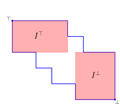
Figure 1: Red rectangles illustrate $I_{M}^{\top}$ and $I_{M}^{\bot}$ of interval $I$.

Definition 3.2 (Construction 1).

For an interval $I_{M}$, we call the smallest rectangle containing it as the bounding rectangle of $I_{M}$. Let $[\mathbf{r}^{\prime},\mathbf{s}^{\prime}]$ be the bounding rectangle of $I_{M}$. Let $\mathbf{r}^{\prime\prime}=\pi_{L(I_{M})}(\mathbf{r}^{\prime})$ and $\mathbf{s}^{\prime\prime}=\pi_{U(I_{M})}(\mathbf{s}^{\prime})$. Let $\mathbf{r}=\frac{1}{2}(\mathbf{r}^{\prime}+\mathbf{r}^{\prime\prime})$ and $\mathbf{s}=\frac{1}{2}(\mathbf{s}^{\prime}+\mathbf{s}^{\prime\prime})$. Let

$$\epsilon_{M}=\max\{\|\mathbf{r}-\mathbf{r^{\prime}}\|_{\infty},\|\mathbf{s}-\mathbf{s^{\prime}}\|_{\infty}\}.$$

Define $\boxed{M}$ to be the rectangle module on $[\mathbf{r},\mathbf{s}]$ if $M$ is not $\epsilon_{M}$-trivializable. Define $\boxed{M}=0$, the trivial module, otherwise. See Figure 2 for an illustration.

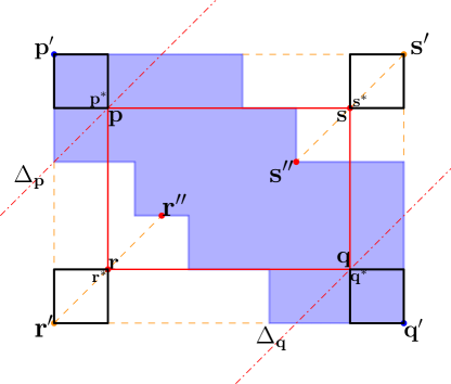
Figure 2: $M=$Blue region. $\boxed{M}=[\mathbf{r},\mathbf{s}]=$red rectangle. The rectangle given by $[\mathbf{r}^{\prime},\mathbf{s}^{\prime}]$ is the bounding rectangle of $I_{M}$. Under the assumption that both $M^{\top}$ and $M^{\bot}$ are not $\epsilon_{M}$-trivializable, the optimal rectangle $R^{*}$ should have four corners contained in the four black boxes corresponding to the four corners of the bounding rectangle, in order to make sure $M|_{\bar{\Delta}_{R^{*}}}$ is $\epsilon_{M}$-trivializable.

We have the following properties for $\boxed{M}$ (proof in A).

Theorem 3.1.

The module $\boxed{M}$ obtained by Construction 1 satisfies the following properties:

1. $d_{\mathrm{{I}}}(M,\boxed{M})\leq\epsilon_{M}$.

2. $d_{\mathrm{{I}}}(M,\boxed{M})=\epsilon_{M}$ if $d_{\mathrm{{I}}}(M,0)\geq\epsilon_{M}$.

3. $\boxed{M}$ is an optimal rectangle module approximating $M$ with respect to $d_{\mathrm{{I}}}$ if both $I_{M}^{\top}$ and $I_{M}^{\bot}$ are large enough to contain a $2\epsilon_{M}\times 2\epsilon_{M}$ square.

We extend our rectangular approximation to interval decomposable modules. For an interval decomposable module $M=\oplus M_{i}$, we extend the definition of $\boxed{M}$ to be $\boxed{M}\triangleq\bigoplus\boxed{M_{i}}$, and let $\epsilon_{M}\triangleq\max\{\epsilon_{M_{i}}\}$. We have the following property, the first one of which follows directly from the definitions.

Proposition 3.2.

For interval decomposable module $M$, $d_{\mathrm{{I}}}(M,\boxed{M})\leq d_{\mathrm{{B}}}(M,\boxed{M})\leq\epsilon_{M}.$

Proposition 3.3.

For two interval decomposable modules $M$ and $N$,

$$d_{\mathrm{{I}}}(M,N)\leq d_{\mathrm{{B}}}(M,N)\leq d_{\mathrm{{B}}}(\boxed{M},\boxed{N})+\epsilon_{M}+\epsilon_{N}\leq 3d_{\mathrm{{I}}}(M,N)+4(\epsilon_{M}+\epsilon_{N}).$$

Proof.

The first inequality is true for any persistence modules. The second inequality comes from triangle inequality. By the stability property of rectangle decomposable modules in Theorem 2.1, $d_{\mathrm{{I}}}(\boxed{M},\boxed{N})\leq d_{\mathrm{{B}}}(\boxed{M},\boxed{N})\leq 3d_{\mathrm{{I}}}(\boxed{M},\boxed{N})$. Using the triangle inequality and Proposition 3.2, we get $d_{\mathrm{{I}}}(\boxed{M},\boxed{N})\leq d_{\mathrm{{I}}}(M,N)+\epsilon_{M}+\epsilon_{N}$. The last inequality immediately follows. ∎

By Proposition 3.2, $d_{\mathrm{{B}}}(M,\boxed{M})$ and $d_{\mathrm{{B}}}(N,\boxed{N})$ are bounded from above by $\epsilon_{M}$ and $\epsilon_{N}$ respectively. Then the question is, what is a closest rectangle decomposable module to $M$ with respect to the bottleneck distance. In line with our previous definition of optimality, we denote $\boxed{M_{i}}^{*}$ to be an optimal rectangle module of the interval module $M_{i}$ under interleaving distance, and set $\boxed{M}^{*}\triangleq\oplus\boxed{M_{i}}^{*}$ to be a rectangle decomposable module approximating $M\simeq\oplus M_{i}$. First we have the following observation which follows from the definifition of the bottleneck distance:

Proposition 3.4.

Given an interval decomposable module $M\simeq\oplus M_{i}$, a rectangle decomposable module $\boxed{M}^{*}\triangleq\oplus\boxed{M_{i}}^{*}$ approximates $M$ optimally with respect to the bottleneck distance.

Therefore, to find an optimal rectangle decomposable module for $M\simeq\oplus M_{i}$ under the bottleneck distance, the question becomes how to find an optimal rectangle approximation for each interval module $M_{i}$.

3.2 An optimal approximation

In Construction 1 (Definition 3.2), we described an approximating rectangle module $\boxed{M}$ for an interval module $M$. By Theorem 3.1, we can observe from Property 3 that $\boxed{M}$ fails to be $\boxed{M}^{*}$ in general case when the top or bottom maximal rectangles of $M$, that is $M^{\top}$ or $M^{\bot}$, is $\epsilon$-trivializable with $\epsilon$ being quite small. In that case, it is more reasonable to ignore these $\epsilon$-trivializable parts to construct a rectangular approximation on the remaining part possibly improving the approximation. Therefore, to compute $\boxed{M}^{*}$, we need to determine what are the top and bottom parts we want to ignore. In this section, we propose an algorithm to compute $\boxed{M}^{*}$ in general case.

First we introduce the Hausdorff distance in infinity norm which is useful in our context. For any set $S\subseteq\mathbb{R}^{2}$ and $\delta\geq 0$, we denote

$$S^{(+\delta)}=\bigcup_{\mathbf{x}\in S}\{\mathbf{x}^{\prime}\in\mathbb{R}^{2}:\|\mathbf{x}-\mathbf{x}^{\prime}\|_{\infty}\leq\delta\}.$$

The Hausdorff distance with the infinity norm between two nonempty sets $S,T\subseteq\mathbb{R}^{n}$ is:

$$d_{\mathrm{{H}}}(S,T)=\inf_{\delta\geq 0}\{S\subseteq T^{(+\delta)}\And T\subseteq S^{(+\delta)}\}.$$

For two nontrivial interval modules $M,N$, we denote $d_{\mathrm{{H}}}(M,N)\triangleq d_{\mathrm{{H}}}(I_{M},I_{N})$. If $N=0$, we set $d_{\mathrm{{H}}}(M,N)\triangleq d_{\mathrm{{I}}}(M,0)$. Given any interval module $M$ and a rectangle module $R$ with $I_{R}$ contained in the bounding rectangle of $I_{M}$, let $\mathbf{p},\mathbf{q}$ be the top-left and bottom-right corner of $I_{R}$ respectively, and $\mathbf{r},\mathbf{s}$ be the bottom-left and top-right corners respectively. Denote the band between two lines $\Delta_{\mathbf{p}}$ and $\Delta_{\mathbf{q}}$ passing through $\mathbf{p}$ and $\mathbf{q}$ respectively, as $\Delta_{R}$, and the complement of $\Delta_{R}$ is denoted as $\bar{\Delta}_{R}$. Observe that $d_{I}(M,R)$ can be calculated as $d_{\mathrm{{I}}}(M,R)=\max\{d_{\mathrm{{I}}}({M|_{\bar{\Delta}_{R}}},0),d_{\mathrm{{I}}}(M|_{\Delta_{R}},R|_{\Delta_{R}})\}$. Notice that we are using $R|_{\Delta R}$ in the above expression even though $R|_{\Delta R}$ has the same underlying interval as $R$, i.e. $I_{R|_{\Delta R}}=I_{R}$ since $I_{R}\subset\Delta_{R}$. We use $R|_{\Delta R}$ because $d_{\mathrm{{I}}}$ is only well defined for modules defined on the same poset. We claim that (proof in  A):

Proposition 3.5.

For $I_{R}$ contained in the bounding rectangle of $I_{M}$,

$$d_{\mathrm{{I}}}(M,R)=\max\{d_{\mathrm{{I}}}({M|_{\bar{\Delta}_{R}}},0),(d_{\mathrm{{I}}}(M|_{\Delta_{R}},0)\vee d_{\mathrm{{I}}}(R|_{\Delta_{R}},0))\wedge d_{\mathrm{{H}}}(M|_{\Delta_{R}},R|_{\Delta_{R}})\}.$$ (1)

The last term can be written explicitly as follows:

Proposition 3.6.

$$d_{\mathrm{{H}}}(M|_{\Delta_{R}},R|_{\Delta_{R}})=\max\{ \mathrm{dl}_{\pm}(\mathbf{p},U(I_{M})),\mathrm{dl}_{\pm}(\mathbf{q},U(I_{M})),\mathrm{dl}_{\pm}(\mathbf{r},L(I_{M})),$$

$$- \mathrm{dl}_{\pm}(\mathbf{p},L(I_{M})),-\mathrm{dl}_{\pm}(\mathbf{q},L(I_{M})),-\mathrm{dl}_{\pm}(\mathbf{s},U(I_{M}))\}.$$

Remark.

For a rectangle module $R$ which does not satisfy the condition that $I_{R}$ is contained in the bounding rectangle of $I_{M}$ as required by Proposition 3.5, we show that there exists a rectangle module $R^{\prime}$ with $I_{R}^{\prime}$ contained in the bounding rectangle of $I_{M}$ such that $d_{I}(M,R^{\prime})\leq d_{\mathrm{{I}}}(M,R)$. This claim is stated and proved as Proposition LABEL:prop:opt_rectangle_in_bounding_rectangle in Appendix.

Based on above observations, now we give the algorithm to compute $\boxed{M}^{*}$. Our algorithm searches a finite partition of $\mathbb{R}^{2}$ to place the four corners of the optimal rectangle while computing the distance between the rectangle and the module in question exactly. Denote $I_{R}=[\mathbf{r},\mathbf{s}]$ with $\mathbf{p},\mathbf{q}$ being its top-left and bottom-right corners respectively. Denote the bounding rectangle of $I_{M}$ as $B$. Consider all the lines $\Delta_{\mathbf{v}},\mathbf{v}\in V(I_{M})$, which partition $B$ into a collection of bands within $B$, denoted as $\mathcal{D}=\{B_{1},B_{2},\cdots,B_{\ell}\}$. The steps of our algorithm are as follows:

1. Compute a finite partition of $B$ with bands in $\mathcal{D}$ as described above.

2. Initialize $\boxed{M}^{*}\leftarrow 0$ to be the zero module.

3. For each quadruple $i,j,k,l$, under constraints $\mathbf{p}\in{B_{i}},\mathbf{q}\in B_{j},\mathbf{r}\in{B_{k}},\mathbf{s}\in{B_{l}}$, find the optimal rectangle approximation $R^{*}=\operatorname*{arg\,min}_{I_{R}=[\mathbf{r},\mathbf{s}]}{d_{\mathrm{{I}}}(M,R)}$ according to the Equation 1 in Proposition 3.5. If $d_{\mathrm{{I}}}(M,R^{*})\leq d_{\mathrm{{I}}}(M,\boxed{M}^{*})$, update $\boxed{M}^{*}\leftarrow R^{*}$.

4. Return $\boxed{M}^{*}.$

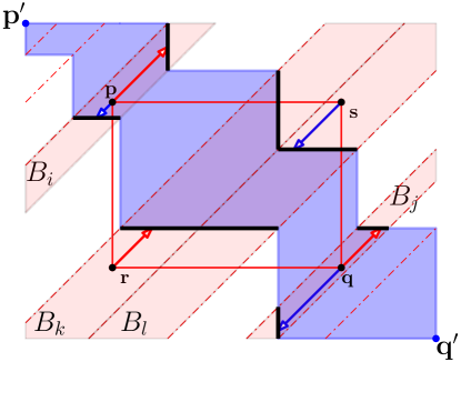
Figure 3: $I_{M}=$Blue region. Red rectangle, $I_{R}=[\mathbf{r},\mathbf{s}]$, is a candidate rectangle with constraints $\mathbf{p}\in B_{i},\mathbf{q}\in B_{j},\mathbf{r}\in B_{k},\mathbf{s}\in B_{l}$. Six arrowed line segments represent the six terms for computing $d_{\mathrm{{H}}}(M|_{\Delta_{R}},R|_{\Delta_{R}})$.

In each iteration of step 3, the optimization problem can be solved by linear programming since all constraints and the terms related to $d_{\mathrm{{I}}}(M,R)$ in Equation 1 can be expressed as linear expressions on the coordinates of $\mathbf{p}=(p_{1},p_{2})$ and $\mathbf{q}=(q_{1},q_{2})$ along with $\max$ and $\min$ operators. For example, $d_{\mathrm{{I}}}(M|_{\bar{\Delta}_{R}},0)=\max\{\|\Delta_{\mathbf{v}}\cap I_{M}\|_{\infty}:\mathbf{v}\in V(I_{M}\cap\bar{\Delta}_{R})\}$ where $\|\Delta_{\mathbf{v}}\cap I_{M}\|_{\infty}$ is the length of the line segment under infinity norm. Essentially these are the longest line segments coming from the intersections between $I_{M}\cap\bar{\Delta}_{R}$ and diagonal lines passing through all vertices of $I_{M}\cap\bar{\Delta}_{R}$. Note that almost all these lengths $\{\|\Delta_{\mathbf{v}}\cap I_{M}\|_{\infty}:\mathbf{v}\in V(I_{M}\cap\bar{\Delta}_{R})\}$ are constant numbers determined by a vertex in $V(I_{M})$ except the ones on the boundary of $\bar{\Delta}_{R}$ which are determined by $\Delta_{\mathbf{p}}$ and $\Delta_{\mathbf{q}}$ that may not pass through any vertex in $V(I_{M})$. These two line segments on the boundary of $\Delta_{R}$ can be represented by linear equations in terms of coordinates of $\mathbf{p}=(p_{1},p_{2})$ and $\mathbf{q}=(q_{1},q_{2})$. For example, $\|\Delta_{\mathbf{p}}\cap I_{M}\|_{\infty}$ can be represented by $\mathrm{dl}_{\pm}(\mathbf{p},U(I_{M}))-\mathrm{dl}_{\pm}(\mathbf{p},L(I_{M}))$. Since $\mathbf{p}$ is within a band $B_{i}$ which is determined by two consecutive vertices of $V(I_{M})$, the intersections $B_{i}\cap U(I_{M}),B_{i}\cap L(I_{M})$ are either horizontal or vertical line segments. If both of them are horizontal or vertical, then $\|\Delta_{\mathbf{p}}\cap I_{M}\|_{\infty}=c$ is a constant number equal to the difference between the coordinates of these two lines. If they are in different directions, say $B_{i}\cap U(I_{M})$ is on the horizontal line $\{y=b\}$ and $B_{i}\cap L(I_{M})$ is on the vertical line $\{x=a\}$, then $\mathrm{dl}_{\pm}(\mathbf{p},U(I_{M}))=b-p_{2}$ and $\mathrm{dl}_{\pm}(\mathbf{p},L(I_{M}))=a-p_{1}$. Therefore, $\|\Delta_{\mathbf{p}}\cap I_{M}\|_{\infty}=b-a-(p_{2}-p_{1})$.

To compute $d_{\mathrm{{I}}}({M|_{\bar{\Delta}_{R}}},0)$ and $d_{\mathrm{{I}}}({M|_{\Delta_{R}}},0)$ efficiently, one can pre-compute $\|\Delta_{\mathbf{v}}\cap I_{M}\|_{\infty}$ for each $\mathbf{v}\in V(I_{M})$ and order them according to $v_{2}-v_{1}$ where $\mathbf{v}=(v_{1},v_{2})$. Then for each pair of $\mathbf{v}_{i},\mathbf{v}_{j}\in V(I_{M})$, compute and store the values

$$\mathrm{Diam}(i,j)\triangleq\max{\{\|\Delta_{\mathbf{v}_{k}}\cap I_{M}\|_{\infty}:i\leq k\leq j\}}\mbox{ and}$$

$$\overline{\mathrm{Diam}}(i,j)\triangleq\max{\{\|\Delta_{\mathbf{v}_{\ell}}\cap I_{M}\|_{\infty}:\ell<i\mbox{ or }\ell>j\}}.$$

This can be done in $O(|V(I_{M})|^{2})$ time. For a given $\Delta_{R}$ between boundaries $\Delta_{\mathbf{p}}$ and $\Delta_{\mathbf{q}}$, we have $\mathbf{v}_{i},\mathbf{v}_{j}\in V(I_{M})\cap\Delta_{R}$ such that $\Delta_{\mathbf{p}}$ is within the band $\Delta_{\mathbf{v}_{i}},\Delta_{\mathbf{v}_{i-1}}$ and $\Delta_{\mathbf{q}}$ is within the band $\Delta_{\mathbf{v}_{j}},\Delta_{\mathbf{v}_{j+1}}$. See Figure 4 for an illustration. Then we have

$$d_{\mathrm{{I}}}({M|_{\bar{\Delta}_{R}}},0)=\|\Delta_{\mathbf{p}}\cap I_{M}\|_{\infty}\vee\|\Delta_{\mathbf{q}}\cap I_{M}\|_{\infty}\vee\mathrm{Diam}(i,j)\mbox{ and}$$

$$d_{\mathrm{{I}}}({M|_{\Delta_{R}}},0)=\|\Delta_{\mathbf{p}}\cap I_{M}\|_{\infty}\vee\|\Delta_{\mathbf{q}}\cap I_{M}\|_{\infty}\vee\overline{\mathrm{Diam}}(i,j).$$

Since we pre-compute and store $\mathrm{Diam}(i,j)$ and $\overline{\mathrm{Diam}}(i,j)$, each iteration incurs only $O(1)$ time for accessing constant number of them.

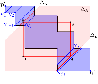
Figure 4: The blue diagonal line segments are $\Delta_{\mathbf{v}}\cap I_{M}$, and the red diagonal line segments are $\Delta_{\mathbf{p}}\cap I_{M}$ and $\Delta_{\mathbf{q}}\cap I_{M}$.

Complexity. Step 3 in the algorithm takes constant time. The last term $d_{\mathrm{{H}}}(M|_{\Delta_{R}},R|_{\Delta_{R}})$ involves constant number of linear equations. The third term $d_{\mathrm{{I}}}(R|_{\Delta_{R}},0)=\min\{q_{1}-p_{1},p_{2}-q_{2}\}$ can be computed in constant time. First two terms $d_{\mathrm{{I}}}(M|_{\bar{\Delta}_{R}},0)$ and $d_{\mathrm{{I}}}(M|_{\Delta_{R}},0)$ can also be evaluated in constant time if we pre-compute the lengths of a collection of line segments as described above. In particular, only two line segments one on each $\Delta_{\mathbf{p}}$ and $\Delta_{\mathbf{q}}$ relate to optimizing variables $\mathbf{p}$ and $\mathbf{q}$ and hence enter into our optimization which can be solved in $O(1)$ time. To see this, observe that the feasible region of $d_{\mathrm{{I}}}(M,R)$ is determined by a constant number of linear equations. An optimal solution is then given by a corner point on the boundary of the feasible region. With a brute-force computation, we can determine all these corner points and then take the optimal one in $O(1)$ time. One can also divide the entire optimization problem into several sub-problems with different feasible regions such that each sub-problem is a min-max problem which can be solved by linear programming, and the optimal solution becomes the minimum over all the solutions of sub-problems. The time complexity still remains $O(1)$ though this division into sub-problems can be more efficient in practice.

With $|\mathcal{D}|=O(|V(I_{M})|)$ being the total number of vertices of the input interval $I$, the time complexity of the whole algorithm is $O(|V(I_{M})|^{4})$.

Now we can compute $\boxed{M}^{*}$ for any interval decomposable module $M=\oplus M_{i}$ by computing $\boxed{M_{i}}^{*}$ for each $i$. We have a result similar to Proposition 3.3 but with a tighter bound on the additional $\epsilon$ terms.

Theorem 3.7.

For two interval decomposable modules $M$ and $N$,

$$d_{\mathrm{{I}}}(M,N)\leq d_{\mathrm{{B}}}(M,N)\leq d_{\mathrm{{B}}}(\boxed{M}^{*},\boxed{N}^{*})+\epsilon_{M}^{*}+\epsilon_{N}^{*}\leq 3d_{\mathrm{{I}}}(M,N)+4(\epsilon_{M}^{*}+\epsilon_{N}^{*})$$

where $\epsilon_{M}^{*}=d_{\mathrm{{B}}}(M,\boxed{M}^{*})$ and $\epsilon_{N}^{*}=d_{\mathrm{{B}}}(N,\boxed{N}^{*})$.

Remark 3.1.

When $M,N$ are rectangle decomposable modules, $\epsilon_{M}^{*}=\epsilon_{N}^{*}=0$. Therefore, our result is a generalization of Bjerkevik’s [Bjerkevik, 2021] stability theorem 2.1.

From this theorem we can see that $\frac{1}{3}d_{\mathrm{{B}}}(M,N)-\frac{4}{3}(\epsilon_{M}^{*}+\epsilon_{N}^{*})\leq d_{\mathrm{{I}}}(M,N)\leq d_{\mathrm{{B}}}(M,N)$. In general, it can be hard to approximate $d_{\mathrm{{I}}}$ by a constant factor. Bjerkevik et al. [Bjerkevik et al., 2020] shows that approximating interleaving distance within a constant factor less than 3 is NP-hard. This additional $\epsilon$ terms may be inevitable in which case this may turn out to be a good polynomial-time computable approximation on $d_{\mathrm{{I}}}$. Also, this bound points to where the gap between $d_{\mathrm{{B}}}$ and $d_{\mathrm{{I}}}$ comes from. These $\epsilon$ terms depend on the structures of $M$ and $N$ themselves, which measure how far an interval decomposable module is from a rectangle decomposable module.

4 Generalized matching distance

In this section, we give an application of our rectangle approximation to define a distance on general 2-parameter persistence modules which can be viewed as a generalization of matching distance [Biasotti et al., 2011, Landi, 2014]. As we know, matching distance and bottleneck distance are most commonly used as a lower and an upper bound respectively for interleaving distance. Following [Landi, 2014], matching distance $d_{\mathrm{{match}}}$ is defined as follows.

Definition 4.1.

For each line $\mathbf{L}$ in $\mathbb{R}^{2}$, use $\mathbf{L}(t)=t\mathbf{a}+\mathbf{b}$ with $a_{1}\vee a_{2}=1,a_{1}\wedge a_{2}>0,b_{1}+b_{2}=0$ as its 1-parameterization over $t\in\mathbb{R}$. For a module $M$, define a 1-parameter persistence module $M_{\mathbf{L}}(t)\triangleq M(\mathbf{L}(t))$. Then

$$d_{\mathrm{{match}}}(M,N)\triangleq\sup_{\mathbf{L}:\mathbf{L}(t)=t\mathbf{a}+\mathbf{b}}(a_{1}\wedge a_{2})d_{\mathrm{{B}}}(M_{\mathbf{L}},N_{\mathbf{L}}).$$

Unfortunately, both matching and bottleneck distances have some drawbacks. Although matching distance can be computed (approximately or exactly [Kerber et al., 2019]) in polynomial time, as indicated in [Cerri et al., 2016, Cerri et al., 2019], it forgets the natural association between the homological properties of slices that are close to each other. On the other hand, the bottleneck distance emphasizes too much on the natural association among slices, which makes the matching obtained by bottleneck distance coherent within each indecomposable component but not stable with respect to the interleaving distance that considers the entire module.

In this section, we propose a general strategy to define a distance $\tilde{d}_{\mathrm{B}}^{\mathcal{C}}$ depending on a chosen convex covering $\mathcal{C}$ on $\mathbb{R}^{2}$ (defined later) which captures the natural association of slices like bottleneck distance but still enjoys some stability-like property based on our previous results as follows

$$d_{\mathrm{{match}}}(M,N)\leq\tilde{d}_{\mathrm{B}}^{\mathcal{C}}(M,N)\leq\min\{3d_{\mathrm{{I}}}(M,N)+\epsilon^{*}(M,N),\,d_{\mathrm{{B}}}(M,N)\}$$ (2)

where $\epsilon^{*}(M,N)$ is determined by the covering $\mathcal{C}$ as

$$\epsilon^{*}(M,N)=4\cdot\sup_{C\in\mathcal{C},\mathbf{a}:a_{1}\wedge a_{2}=1}d_{\mathrm{{B}}}(M^{\mathbf{a}}|_{C},\boxed{M^{\mathbf{a}}|_{C}}^{*})+d_{\mathrm{{B}}}(N^{\mathbf{a}}|_{C},\boxed{N^{\mathbf{a}}|_{C}}^{*}).$$ (3)

Here $M^{\mathbf{a}}$ is a scaled module of $M$ defined as

Definition 4.2.

$M^{\mathbf{a}}(\mathbf{u})=M(\mathbf{u}\odot\mathbf{a})$ where $\mathbf{u}\odot\mathbf{a}=(u_{1}a_{1},u_{2}a_{2})$ known to be the Hadamard product. See Figure 5 for an illustration.

By carefully choosing the covering $\mathcal{C}_{\alpha}$ for any $\alpha\in[0,1]$, we can further get a distance $\tilde{d}_{\mathrm{B}}^{\mathcal{C}_{\alpha}}$ that enjoys $(3+\alpha)$-stability as follows:

$$d_{\mathrm{{match}}}(M,N)\leq\tilde{d}_{\mathrm{B}}^{\mathcal{C}_{\alpha}}(M,N)\leq\min\{(3+\alpha)d_{\mathrm{{I}}}(M,N),\;d_{\mathrm{{B}}}(M,N)\}.$$ (4)

We will show that the matching distance can be viewed as a special case of our construction when $\mathcal{C}$ is chosen to be the set containing all slope-1 lines in $\mathbb{R}^{2}$. The main idea is to cover the entire plane $\mathbb{R}^{2}$ by some collection of bands $\mathcal{C}$. By carefully choosing these bands we make sure that the restricted modules $M|_{C}$ and $N|_{C}$ within each band $C\in\mathcal{C}$ are interval decomposable. Then, locally we can compute the bottleneck distance which bounds the interleaving distance in each band according to our previous results. As in [Cerri and Frosini, 2011], our proposed distance can be approximated by choosing a finite set of directions. Recently, in [Kerber et al., 2019], a polynomial time algorithm has been presented for computing the matching distance exactly. It remains open if our proposed distance can also be computed exactly using similar ideas.

We call a set $\mathcal{C}$ of convex sets a convex covering of $\mathbb{R}^{2}$ if the union of the sets of $\mathcal{C}$ equals $\mathbb{R}^{2}$. For any convex set $C\subseteq\mathbb{R}^{n}$, we have induced $C$-modules $M|_{C}$ and $N|_{C}$. Therefore, we can define $d_{\mathrm{{I}}}(M|_{C},N|_{C})$ with the following property:

Fact 2.

For two convex sets $C$ and $C^{\prime}$, if $C^{\prime}\subseteq C$, then $d_{\mathrm{{I}}}(M|_{C^{\prime}},N|_{C^{\prime}})\leq d_{\mathrm{{I}}}(M|_{C},N|_{C})$.

We need the following definitions for further development.

Definition 4.3.

Define $\mathrm{Cov}(\mathbb{R}^{2})\triangleq\{\mathcal{C}\mid\mathcal{C}\mbox{ is a convex covering on }\mathbb{R}^{2}\}$. For two convex coverings $\mathcal{C}\mbox{ and }\mathcal{C}^{\prime}$, we say $\mathcal{C}^{\prime}$ is a refinement of $\mathcal{C}$, denoted as $\mathcal{C}^{\prime}\subseteq\mathcal{C}$, if $\forall C^{\prime}\in\mathcal{C}^{\prime},\exists C\in\mathcal{C},C^{\prime}\subseteq C$. For $\mathcal{C}\in\mathrm{Cov}(\mathbb{R}^{2})$, define $d_{\mathrm{{I}}}^{\mathcal{C}}(M,N)\triangleq\sup_{C\in\mathcal{C}}d_{\mathrm{{I}}}(M|_{C},N|_{C})$ and $d_{\mathrm{{B}}}^{\mathcal{C}}(M,N)\triangleq\sup_{C\in\mathcal{C}}d_{\mathrm{{B}}}(M|_{C},N|_{C})$ .

Remark 4.1.

The refinement relation defines a partial order on $\mathrm{Cov}(\mathbb{R}^{2})$. The minumum covering is the discrete covering consisting of all singleton sets of $\mathbb{R}^{2}$. The maximum covering is $\{\mathbb{R}^{2}\}$. Furthermore, $d_{\mathrm{{I}}}^{(\cdot)}$ can be viewed as an order preserving mapping from poset $\mathrm{Cov}(\mathbb{R}^{2})$ to pseudometric functions on bimodules. That is,

Proposition 4.1.

For $\mathcal{C}^{\prime}\leq\mathcal{C}\in\mathrm{Cov}(\mathbb{R}^{2})$, $d^{\mathcal{C^{\prime}}}_{I}\leq d^{\mathcal{C}}_{I}$. Specifically, $d_{\mathrm{{I}}}^{\{\mathbb{R}^{2}\}}=d_{\mathrm{{I}}}$ and $d_{\mathrm{{B}}}^{\{\mathbb{R}^{2}\}}=d_{\mathrm{{B}}}$.

Most of $d_{\mathrm{{I}}}^{\mathcal{C}}$ are hard to analyze in general which prompts us to construct some special covering $\mathcal{C}$. Consider a finite subset $\mathbf{S}=\{\mathbf{s}^{(1)},\mathbf{s}^{(2)},\cdots,\mathbf{s}^{(l)}\}\subset\mathbb{R}^{2}$ ordered by $\Delta_{\mathbf{s}^{(i)}}$, which means $\mathbf{s}^{(i)}\leq\mathbf{s}^{(j)}$ if $s^{(i)}_{2}-s^{(i)}_{1}\leq s^{(j)}_{2}-s^{(j)}_{1}$. All these $\Delta_{\mathbf{s}^{(i)}}$ partition $\mathbb{R}^{2}$ into finitely many regions. We collect all these regions with boundaries to construct the covering $\mathcal{C}_{\mathbf{S}}$ for the set $\mathbf{S}$. For $\mathbf{S}=\emptyset$, we define $\mathcal{C}_{\emptyset}=\{\mathbb{R}^{2}\}$. We extend our notation to incorporate the special set $\mathbf{S}=\mathbb{R}^{2}$ by defining $\mathcal{C}_{\mathbb{R}^{2}}=\{\Delta_{\mathbf{s}}\mid\mathbf{s}\in\mathbb{R}^{2}\}$, which is the collection of all diagonal lines in $\mathbb{R}^{2}$. By Proposition 4.1, we immediately have

Proposition 4.2.

For any finite set $\mathbf{S}\subset\mathbb{R}^{2}$, $\mathcal{C}_{\mathbb{R}^{2}}\leq\mathcal{C}_{\mathbf{S}}\leq\mathcal{C}_{\emptyset}$.

Before we define our generalized matching distance, we need another notation. Let $\mathbf{A}=\{\mathbf{a}=(a_{1},a_{2})\in\mathbb{R}^{2}_{+}\mid a_{1}\wedge a_{2}=1\}$. For a vector $\mathbf{a}=(a_{1},a_{2})\in\mathbf{A}$, recall that the scaled module $M^{\mathbf{a}}$ of $M$ is $M^{\mathbf{a}}(\mathbf{u})\triangleq M(\mathbf{a}\odot\mathbf{u})=M(a_{1}\cdot u_{1},a_{2}\cdot u_{2})$ (Figure 5). Note that $M^{(1,1)}=M$. Similarly, we also define the scaled covering $\mathcal{C}_{\mathbf{S}}^{\mathbf{a}}\triangleq\mathcal{C}_{\mathbf{a}^{-1}\odot\mathbf{S}}$ for a covering $\mathcal{C}_{\mathbf{S}}$, where ${\mathbf{a}^{-1}\odot\mathbf{S}}=\{\mathbf{a}^{-1}\odot\mathbf{s}\mid\mathbf{s}\in\mathbf{S}\}$. Intuitively, scaled modules and scaled coverings together account for all directions $\mathbf{a}\in\mathbf{A}$ needed to be considered for matching distance even though coverings align along the diagonal direction.

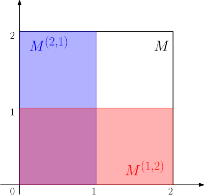
Figure 5: $M$ is a module on $[0,2]\times[0,2]$, the blue region and red region are the underlying intervals of $M^{(2,1)}$ and $M^{(1,2)}$ respectively.

Now we construct the generalized matching distance.

Definition 4.4.

Given a covering $\mathcal{C}_{\mathbf{S}}$, for two persistence modules $M,N$, define

$$\tilde{d_{\mathrm{{I}}}}^{\mathcal{C}_{\mathbf{S}}}(M,N)\triangleq\sup_{\mathbf{a}\in\mathbf{A}}d_{\mathrm{{I}}}^{\mathcal{C}_{\mathbf{S}}^{\mathbf{a}}}(M^{\mathbf{a}},N^{\mathbf{a}})=\sup_{\mathbf{a}\in\mathbf{A}}\sup_{C\in\mathcal{C}_{\mathbf{S}}^{\mathbf{a}}}d_{\mathrm{{I}}}(M^{\mathbf{a}}|_{C},N^{\mathbf{a}}|_{C})$$

and

$$\tilde{d_{\mathrm{{B}}}}^{\mathcal{C}_{\mathbf{S}}}(M,N)\triangleq\sup_{\mathbf{a}\in\mathbf{A}}d_{\mathrm{{B}}}^{\mathcal{C}_{\mathbf{S}}^{\mathbf{a}}}(M^{\mathbf{a}},N^{\mathbf{a}})=\sup_{\mathbf{a}\in\mathbf{A}}\sup_{C\in\mathcal{C}_{\mathbf{S}}^{\mathbf{a}}}d_{\mathrm{{B}}}(M^{\mathbf{a}}|_{C},N^{\mathbf{a}}|_{C}).$$

Based on our definition, we have the following properties:

Proposition 4.3.

1. For $\mathcal{C}_{\mathbf{S}^{\prime}}\leq\mathcal{C}_{\mathbf{S}}$, $\tilde{d_{\mathrm{{I}}}}^{\mathcal{C}_{\mathbf{S}^{\prime}}}\leq\tilde{d_{\mathrm{{I}}}}^{\mathcal{C}_{\mathbf{S}}}$ and $\tilde{d_{\mathrm{{B}}}}^{\mathcal{C}_{\mathbf{S}^{\prime}}}\leq\tilde{d_{\mathrm{{B}}}}^{\mathcal{C}_{\mathbf{S}}}$;
2. $\tilde{d}_{\mathrm{I}}^{\mathcal{C}_{\mathbb{R}^{2}}}=\tilde{d}_{\mathrm{B}}^{\mathcal{C}_{\mathbb{R}^{2}}}=d_{\mathrm{{match}}}$;
3. $\tilde{d}_{\mathrm{I}}^{\mathcal{C}_{\emptyset}}=d_{\mathrm{{I}}},\tilde{d}_{\mathrm{B}}^{\mathcal{C}_{\emptyset}}=d_{\mathrm{{B}}}$.

Proof.

The first one is an immediate corollary from Proposition 4.1. Consider the second one. The first equality comes from isometry theorem of 1-parameter persistence module. To show the second equality, recall Definition 4.1 of $d_{\mathrm{{match}}}$:

$$d_{\mathrm{{match}}}(M,N)\triangleq\sup_{\begin{subarray}{c}\mathbf{L}:\mathbf{L}(t)=t\mathbf{a}+\mathbf{b},\\ a_{1}\vee a_{2}=1,\\ a_{1}\wedge a_{2}>0,\\ b_{1}+b_{2}=0\end{subarray}}(a_{1}\wedge a_{2})d_{\mathrm{{B}}}(M_{\mathbf{L}},N_{\mathbf{L}})$$

where $M_{\mathbf{L}}$ is defined by $M_{\mathbf{L}}(t)=M(\mathbf{L}(t))$.

First, note that, in the definition of $d_{\mathrm{{match}}}$, we can remove the scalar weight term $(a_{1}\wedge a_{2})$ by changing parameterization of $\mathbf{L}(t)$ with $a_{1}\wedge a_{2}=1,b_{1}+b_{2}=0$. Now we obtain an equivalent definition of $d_{\mathrm{{match}}}$ as follows.

$$d_{\mathrm{{match}}}(M,N)=\sup_{\begin{subarray}{c}\mathbf{L}:\mathbf{L}(t)=t\mathbf{a}+\mathbf{b},\\ a_{1}\wedge a_{2}=1,\\ b_{1}+b_{2}=0\end{subarray}}d_{\mathrm{{B}}}(M_{\mathbf{L}},N_{\mathbf{L}}).$$

For each $\mathbf{L}$, let $\mathbf{L}^{\prime}\triangleq\mathbf{a}^{-1}\odot\mathbf{L}$ given by $\mathbf{L}^{\prime}(t)=t(1,1)+\mathbf{a}^{-1}\odot\mathbf{b}$. Observe that

$$M^{\mathbf{a}}|_{\mathbf{L}^{\prime}}(\mathbf{L}^{\prime}(t))=M(\mathbf{a}\odot\mathbf{L}^{\prime}(t))=M(\mathbf{a}\odot\mathbf{a}^{-1}\odot\mathbf{L}(t))=M(\mathbf{L}(t))=M_{\mathbf{L}}(t).$$

This means $\forall\mathbf{L}:\mathbf{L}(t)=t\mathbf{a}+\mathbf{b}$, the 1-parameter module $M_{\mathbf{L}}$ and the corresponding $\mathbf{a}$-scaled model $\mathbf{L}^{\prime}$-module $M^{\mathbf{a}}|_{\mathbf{L}^{\prime}}$ are the same in the sense that $\forall t,M_{\mathbf{L}}(t)=M^{\mathbf{a}}|_{\mathbf{L}^{\prime}}(\mathbf{L}^{\prime}(t))$. It is not difficult to check that the corresponding linear maps are also the same. Taking the supremum over all lines $\mathbf{L}$, we get $d_{\mathrm{{match}}}=\tilde{d}_{\mathrm{B}}^{\mathcal{C}_{\mathbb{R}^{2}}}$ by definition.

For the third one, the second equality is an immediate result from the first equality. For the first equality, we need to show that $d_{\mathrm{{I}}}(M^{\mathbf{a}},N^{\mathbf{a}})\leq d_{\mathrm{{I}}}(M,N),\forall\mathbf{a}$. Assume $M,N$ are $\delta$-interleaved with interleaving morphisms $\phi:M\rightarrow N_{\rightarrow\vec{\delta}}$ and $\psi:N\rightarrow M_{\rightarrow\vec{\delta}}$. We claim that $M^{\mathbf{a}},N^{\mathbf{a}}$ are $\delta$-interleaved witnessed by maps $\phi^{\mathbf{a}}$ and $\psi^{\mathbf{a}}$ between $M^{\mathbf{a}}$ and $N^{\mathbf{a}}$ constructed as follows.

$$\phi^{\mathbf{a}}(\mathbf{x}):= N(\mathbf{a}\odot\mathbf{x}+\vec{\delta}\rightarrow\mathbf{a}\odot\mathbf{x}+\mathbf{a}\odot\vec{\delta})\circ\phi(\mathbf{a}\odot\mathbf{x})$$

$$\psi^{\mathbf{a}}(\mathbf{x}):= M(\mathbf{a}\odot\mathbf{x}+\vec{\delta}\rightarrow\mathbf{a}\odot\mathbf{x}+\mathbf{a}\odot\vec{\delta})\circ\psi(\mathbf{a}\odot\mathbf{x})$$

Notice that $\mathbf{a}$ satisfies $a_{1}\wedge a_{2}=1$. So, $\mathbf{a}\odot\mathbf{x}+\vec{\delta}\leq\mathbf{a}\odot\mathbf{x}+\mathbf{a}\odot\vec{\delta}$. Therefore, all the arrows ‘$\rightarrow$’ above are well-defined. The construction for $\phi^{\mathbf{a}},\psi^{\mathbf{a}}$ are symmetric. By commutative properties of $\phi,\psi$ and linear maps within $M$ and $N$, it can be verified that $\phi^{\mathbf{a}},\psi^{\mathbf{a}}$ indeed provide $\delta$-interleaving between $M^{\mathbf{a}}$ and $N^{\mathbf{a}}$. We leave details in LABEL:sec:missing_proofs2. ∎

Therefore, $d_{\mathrm{{match}}}$ can be viewed as a special case which bounds $\tilde{d}_{\mathrm{I}}$ and $\tilde{d}_{\mathrm{B}}$ from below. Computing $\tilde{d}_{\mathrm{I}}$ or $\tilde{d_{\mathrm{{B}}}}$ in general can be intractable. For some $\mathcal{C}_{\mathbf{S}}$ constructed in a specific way, we provide an efficient algorithm to approximate $\tilde{d}_{\mathrm{I}}^{\mathcal{C}_{\mathbf{S}}}$ by a finite subset $\hat{\mathbf{A}}\subseteq\mathbf{A}$. The idea is to construct a set $\mathbf{S}$ for $M,N$ so that for any $\mathbf{a}\in\mathbf{A}$ and any $C\in\mathcal{C}_{\mathbf{S}}^{\mathbf{a}}$, both $M^{\mathbf{a}}|_{C}$ and $N^{\mathbf{a}}|_{C}$ are interval decomposable. Based on such a set $\mathbf{S}$, we can approximate $\tilde{d}_{\mathrm{B}}$ efficiently and utilize the results in the previous section to bound $\tilde{d}_{\mathrm{I}}$. Before we give the construction of the set $\mathbf{S}$, we first introduce the results and the algorithm.

Proposition 4.4.

Given two modules $M,N$ and a covering $\mathcal{C}_{\mathbf{S}}$ such that $\forall\mathbf{a}\in\mathbf{A},\forall C\in\mathcal{C}_{\mathbf{S}}^{\mathbf{a}}$, both $M^{\mathbf{a}}|_{C}$ and $N^{\mathbf{a}}|_{C}$ are interval decomposable, we have

$$d_{\mathrm{{match}}}(M,N)\leq\tilde{d}_{\mathrm{I}}^{\mathcal{C}_{\mathbf{S}}}(M,N)\leq\tilde{d}_{\mathrm{B}}^{\mathcal{C}_{\mathbf{S}}}(M,N) \leq\min\{3\tilde{d}_{\mathrm{I}}^{\mathcal{C}_{\mathbf{S}}}(M,N)+\epsilon^{*}(M,N),d_{\mathrm{{B}}}(M,N)\}$$ (5)

$$\leq\min\{3d_{\mathrm{{I}}}(M,N)+\epsilon^{\mathcal{C}_{\mathbf{S}}}(M,N),d_{\mathrm{{B}}}(M,N)\}$$ (6)

where

$$\epsilon^{\mathcal{C}_{\mathbf{S}}}(M,N)=4\cdot\sup_{C\in\mathcal{C}_{\mathbf{S}},\mathbf{a}\in\mathbf{A}}d_{\mathrm{{B}}}(M^{\mathbf{a}}|_{C},\boxed{M^{\mathbf{a}}|_{C}}^{*})+d_{\mathrm{{B}}}(N^{\mathbf{a}}|_{C},\boxed{N^{\mathbf{a}}|_{C}}^{*}).$$ (7)

The distance $\tilde{d}_{\mathrm{B}}^{\mathcal{C}_{\mathbf{S}}}$ is defined as a supremum over all scaled modules $M^{\mathbf{a}}$ and $N^{\mathbf{a}}$ for every $\mathbf{a}\in\mathbf{A}$. To develop a polynomial time approximation algorithm, following [Cerri and Frosini, 2011], we take a finite subset $\hat{\mathbf{A}}\subseteq\mathbf{A}$ to approximate the distance. We summarize the algorithm for approximating $\tilde{d}_{\mathrm{B}}$:

1. Compute the minimal presentations of $M$ and $N$ by the algorithm given in [Lesnick and Wright, 2019].

2. Compute the decomposition $M\simeq\oplus M_{i}$ and $N\simeq\oplus N_{j}$ by the algorithm given in [Dey and Xin, 2019].

3. For every non-interval component $M_{i}$ and $N_{j}$, select a set $\mathbf{S}\subseteq\mathbb{R}^{2}$ satisfying the premise of Proposition 4.4 and construct $\mathcal{C}_{\mathbf{S}}$. Take the union over all these sets of $\mathbf{S}$’s.

4. For $\forall\mathbf{a}\in\hat{\mathbf{A}},\forall C\in\mathcal{C}_{\mathbf{S}}^{\mathbf{a}}$, compute the bottleneck distance $d_{\mathrm{{B}}}(M^{\mathbf{a}}|_{C},N^{\mathbf{a}}|_{C})$ by the algorithm given in [Dey and Xin, 2018].

5. Output $\displaystyle\max_{\mathbf{a}\in\hat{\mathbf{A}},\Delta_{C}\in\Delta_{\mathcal{C}_{\mathbf{S}}^{\mathbf{a}}}}d_{\mathrm{{B}}}(M^{\mathbf{a}}|_{C},N^{\mathbf{a}}|_{C})$ as an approximation of $\tilde{d}_{\mathrm{B}}^{\mathcal{C}_{\mathbf{S}}}(M,N)$.

The upper bound in Proposition 4.4 can be improved for some special covering.

Corollary 4.5.

Let $\mathcal{C}_{\mathbf{S}}$ be a covering satisfying the condition in Proposition 4.4 and let $\mathcal{C}_{\mathbf{S}^{\prime}}\subset\mathcal{C}_{\mathbf{S}}$ be a refinement such that $\epsilon^{\mathcal{C}_{\mathbf{S}^{\prime}}}(M,N)\leq\alpha d_{\mathrm{{match}}}(M,N)$, then we have

$$d_{\mathrm{{match}}}(M,N)\leq\tilde{d}_{\mathrm{B}}^{\mathcal{C}_{\mathbf{S}^{\prime}}}(M,N)\leq\min\{(3+\alpha)\cdot d_{\mathrm{{I}}}(M,N),\,d_{\mathrm{{B}}}(M,N)\}.$$ (8)

Such a refinement $\mathcal{C}_{\mathbf{S}^{\prime}}$ can simply be obtained as follows. Each $C\in\mathcal{C}_{\mathbf{S}}$, which does not satisfy the condition that $4\sup_{\mathbf{a}\in\mathbf{A}}[d_{\mathrm{{B}}}(M^{\mathbf{a}}|_{C},\boxed{M^{\mathbf{a}}|_{C}}^{*})+d_{\mathrm{{B}}}(N^{\mathbf{a}}|_{C},\boxed{N^{\mathbf{a}}|_{C}}^{*})]\leq\alpha d_{\mathrm{{match}}}(M,N)$, is subdivided evenly into several bands $C_{i}$’s so that $2\epsilon_{C_{i}}\leq\alpha d_{\mathrm{{match}}}(M,N)$. Thanks to Proposition LABEL:prop:subdivide_bound in LABEL:sec:missing_proofs2, we get that

$$4\sup_{C_{i}}\sup_{\mathbf{a}\in\mathbf{A}}d_{\mathrm{{B}}}(M^{\mathbf{a}}|_{C_{i}},\boxed{M^{\mathbf{a}}|_{C_{i}}}^{*})+d_{\mathrm{{B}}}(N^{\mathbf{a}}|_{C_{i}},\boxed{N^{\mathbf{a}}|_{C_{i}}}^{*})\leq\alpha d_{\mathrm{{match}}}(M,N).$$

Now $\mathcal{C}_{\mathbf{S}^{\prime}}$ as constructed above satisfies that $\epsilon^{\mathcal{C}_{\mathbf{S}^{\prime}}}(M,N)\leq\alpha d_{\mathrm{{match}}}(M,N)$. If $C$ is an infinity band (not bounded by two lines), one can subdivide $C$ starting from the lower or upper boundary iteratively until the condition is satisfied.

Remark.

From above constructions, we can see that the choice of covering $\mathcal{C}$ gives a trade-off between lower and upper bounds. Finer construction gives us a distance closer to the matching distance $d_{\mathrm{{match}}}$, while coarser construction provides a distance which is closer to the bottleneck distance $d_{\mathrm{{B}}}$.

Now we discuss how to construct the set $\mathbf{S}$ in step 3 which should satisfy the premise of Proposition 4.4. For this we need the idea of finite presentation which is well studied in commutative algebra for structures like graded modules. Here we follow the description in [Kerber et al., 2019] to give a more intuitive definition of finite presentation as a graded matrix which does not require too much background in commutative algebra (one can check [Atiyah, 2018, Cox et al., 2006, Lesnick, 2015] for more details about finite presentation).

For any band described before $C\subset\mathbb{R}^{2}$, a finite presentation is an $n\times m$ matrix $P$ over field ${\mathbb{F}}_{2}$, where each row $i$ is labeled by a point $\mathrm{gr}({\mathrm{row}}_{i})\in C$, and each column $j$ is labeled by a point $\mathrm{gr}({\mathrm{col}}_{j})\in C$, called the grades, such that $P_{i,j}=1\implies\mathrm{gr}({\mathrm{row}}_{i})\leq\mathrm{gr}({\mathrm{col}}_{j})$. We denote all grades of rows as $\mathrm{gr}({\mathrm{row}}P)$ and all grades of columns as $\mathrm{gr}({\mathrm{col}}P)$. The grades $\mathrm{gr}({\mathrm{row}}P)$ and $\mathrm{gr}({\mathrm{col}}P)$ represent generators and relations of a persistence module constructed as follows: Let $e_{1},e_{2},\cdots,e_{l}$ denote the standard basis of ${\mathbb{F}}_{2}^{l}$. For any $\mathbf{u}\in{C}$, define the subset $\mathrm{Gen}(\mathbf{u})\triangleq\{e_{i}\mid\mathrm{gr}({\mathrm{row}}_{i})\leq\mathbf{u}\}$ and $\mathrm{Rel}(\mathbf{u})\triangleq\{{\mathrm{col}}_{j}\mid\mathrm{gr}({\mathrm{col}}_{j})\leq\mathbf{u}\}$. Then define $M^{P}(\mathbf{u})=\mathrm{Span}(\mathrm{Gen}(\mathbf{u}))/\mathrm{Span}(\mathrm{Rel}(\mathbf{u}))$, and $M^{P}(\mathbf{u}\rightarrow\mathbf{v})$ as the map induced by the inclusion map $\mathrm{Span}(\mathrm{Gen}(\mathbf{u}))\rightarrow\mathrm{Span}(\mathrm{Gen}(\mathbf{v}))$. It can be checked that $M^{P}$ is a $C$- module. If $M^{P}$ is isomorphic to some persistence module $M$, we say $P$ is a presentation matrix of $M$.

Remark.

Note that our definition above is consistent with the one in [Kerber et al., 2019] for $C=\mathbb{R}^{2}$. We extend it for all band posets we care about here. In practice, the data is often given as a simplicial filtration which induces the persistence module. It is shown in [Lesnick and Wright, 2019] that for a $2$-parameter persistence module, a finite presentation can be computed in cubic time.

Note that $\mathrm{gr}({\mathrm{col}}P)$ and $\mathrm{gr}({\mathrm{row}}P)$ are two subsets of $\mathbb{R}^{2}$ with partial order naturally induced from $\mathbb{R}^{2}$. Specifically, we claim the following Proposition for an important special case (proof in LABEL:sec:missing_proofs2)

Proposition 4.6.

If $P$ is a presentation of $M$ such that neither $\mathrm{gr}({\mathrm{col}}P)$ nor $\mathrm{gr}({\mathrm{row}}P)$ has incomparable pairs, then $M$ is interval decomposable.

Observe that the Proposition above provides only a sufficient condition for interval decomposable modules. It is not a necessary condition.

Borrowing an idea from [Lesnick and Wright, 2015], for any persistence module $M$ with finite presentation $P$, and for any band $C$ with upper and lower boundary $\Delta_{a}$ and $\Delta_{b}$ respectively for some $-\infty\leq a\leq b\leq+\infty$ ($a=-\infty$ means $C$ has no lower boundary, $b=+\infty$ means $C$ has no upper boundary), define a $\mathrm{push}$ operation on any point $\mathbf{u}\in\mathbb{R}^{2}$ to band $C$ as:

$$\mathrm{push}_{C}(\mathbf{u}=(u_{1},u_{2}))\triangleq\min\{\mathbf{w}\in C\mid\mathbf{w}\leq\mathbf{u}\}=\begin{cases}(u_{2}-b,u_{2})\mbox{ if }\mathbf{u}\mbox{ is above }\Delta_{b},\\ (u_{1},u_{1}+a)\mbox{ if }\mathbf{u}\mbox{ is below }\Delta_{a},\\ \mathbf{u}\mbox{ if }\mathbf{u}\in C.\end{cases}$$ (9)

Intuitively, $\mathrm{push}_{C}(\mathbf{u})$ is the lower-left corner of the intersection between $C$ and the unbounded rectangle $[\mathbf{u},(+\infty,+\infty)]$. See Figure 6 as an illustration.

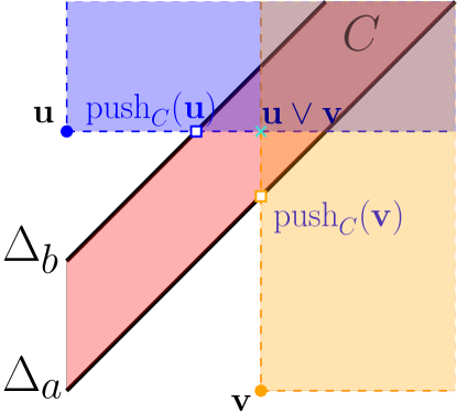
Figure 6: Examples of $\mathrm{push}_{C}$ of two points $\mathbf{u},\mathbf{v}$. The square points are $\mathrm{push}_{C}(\mathbf{u}),\mathrm{push}_{C}(\mathbf{v})$.

Now we claim the following Proposition to connect the finite presentation between $M$ and $M|_{C}$ (proof in LABEL:sec:missing_proofs2).

Proposition 4.7.

Given a presentation of $M$ with finite presentation $P$ and a band $C$, the restriction $M|_{C}$ has a finite presentation $P$ which can be obtained by replacing each $\mathbf{u}$ of $P$ with $\mathrm{push}_{C}(\mathbf{u})\triangleq\min\{\mathbf{w}\in C\mid\mathbf{w}\leq\mathbf{u}\}$.

Now given persistence modules $M$ and $N$ with finite presentations $P_{M}$ and $P_{N}$ respectively, let $Gr=\{\mathrm{gr}({\mathrm{row}}P_{M}),\mathrm{gr}({\mathrm{col}}P_{M}),\mathrm{gr}({\mathrm{row}}P_{N}),\mathrm{gr}({\mathrm{col}}P_{N})\}$. Let $\mathbf{S}=\{\mathbf{u}\vee\mathbf{v}\triangleq(u_{2}\vee v_{2},u_{1}\vee v_{1})\mid\mathbf{u},\mathbf{v}\mbox{ are incomparable in }G\mbox{ for }G\in Gr\}$ be the anchor set. As an immediate result from Proposition 4.6, we have the following property which satisfies the requirement in Proposition 4.4.

Proposition 4.8.

Given a persistent module $M$ with finite presentation $P$, let $\mathbf{S}\triangleq\{\mathbf{u}\vee\mathbf{v}\triangleq(u_{2}\vee v_{2},u_{1}\vee v_{1})\mid\mathbf{u},\mathbf{v}\mbox{ are incomparable in }\mathrm{gr}({\mathrm{row}}P_{M})\mbox{ or }\mathrm{gr}({\mathrm{col}}P)\}$, then we have $\forall\mathbf{a},C\in\mathcal{C}_{\mathbf{S}}$, $M^{\mathbf{a}}|_{C}$ is interval decomposable.

5 Conclusion

In this paper, first we consider interval decomposable modules and their optimal approximations with rectangle decomposable modules with respect to the bottleneck distance. We present a polynomial time algorithm for computing this optimal approximation exactly which, together with the polynomial-time computable bottleneck distance among interval decomposable modules [Dey and Xin, 2018], provides a lower bound on the interleaving distance. Next, we propose a distance between $2$-parameter persistence modules that is more discriminating than the matching distance and is bounded from above by the bottleneck distance. This distance can be approximated by a polynomial time algorithm. Using an approach in [Kerber et al., 2019], it may be plausible to compute it exactly–a question we leave open for future research. This distance can bound the interleaving distance from below with some subtractive factors derived from our optimal approximation of interval decomposable modules with rectangle decomposable modules. For this, we propose a non-trivial covering of a given module by interval decomposable modules which can be an interesting technique on its own.

Appendix A Missing proofs in Section 3

First, we introduce some definitions and results used later in our proof. Most of them comes from [Dey and Xin, 2018].

Definition A.1 (Valid intersection).

An intersection component $Q_{i}$ is $(M,N)$-valid (or valid in short if the order of the modules is clear from the context) if for each $\mathbf{x}\in I_{Q_{i}}$ the following two conditions hold (see Figure 7):

$$\mbox{(i) }\mathbf{y}\leq\mathbf{x}\mbox{ and }\mathbf{y}\in I_{M}\implies\mathbf{y}\in I_{N},\mbox{ and (ii) }\mathbf{z}\geq\mathbf{x}\mbox{ and }\mathbf{z}\in I_{N}\implies\mathbf{z}\in I_{M}.$$

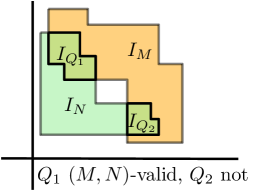
Figure 7: Examples of a valid intersection and an invalid intersection.

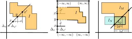
Figure 8: $d=\mathrm{dl}(x,I)$, $y=\pi_{I}(x)$, $d^{\prime}=\mathrm{dl}(x^{\prime},L(I))$ (left); $d=\mathrm{dl}(x,I)$ and $d^{\prime}=\mathrm{dl}(x^{\prime},U(I))$ are defined on the left edge of $B(\bar{\mathbb{R}}^{2})$ (middle); $Q$ is $d^{\prime}_{(M,N)}$- and $d_{(N,M)}$-trivializable (right).

Definition A.2 (Trivializable intersection).

Let $Q$ be a connected component of the intersection of two modules $M$ and $N$. For each point $\mathbf{x}\in I_{Q}$, define

$$d^{(M,N)}_{triv}(\mathbf{x})=\max\{\mathrm{dl}(\mathbf{x},U(I_{M}))/2,\mathrm{dl}(\mathbf{x},L(I_{N}))/2)\}.$$

For $\delta\geq 0$, we say a point $\mathbf{x}$ is $\delta_{(M,N)}$-trivializable if $d^{(M,N)}_{triv}(\mathbf{x})<\delta$. We say an intersection component $Q$ is $\delta_{(M,N)}$-trivializable (or trivializable for brief if the order of modules is clear from context) if each point in $I_{Q}$ is $\delta_{(M,N)}$-trivializable (Figure 8). We also denote $d_{triv}^{(M,N)}(I_{Q}):=\sup_{\mathbf{x}\in I_{Q}}{\{d_{triv}^{(M,N)}(\mathbf{x})\}}.$

Note that if we set $N=M$, and let $Q=M$ be the only connected component of intersection of $M$ and $N$, then $d_{triv}^{M,M}(I_{M})=d_{\mathrm{{I}}}(M,0)$. We say $M$ is $\delta$-trivializable if $\delta\geq d_{\mathrm{{I}}}(M,0)$.

Definition A.3.

Given an interval module $M$ and the diagonal line $\Delta_{\mathbf{x}}$ for any $\mathbf{x}\in\mathbb{R}^{2}$, let $\mathbf{L}(t)=t\cdot(1,1)+0.5\cdot(-c,c)$ as the parameterization of line $\Delta_{\mathbf{x}}$ with $c=x_{2}-x_{1}$ being the vertical intercept of $\Delta_{\mathbf{x}}$. We define 1-parameter slice of $M$ along $\Delta_{\mathbf{x}}$, denoted as $M|_{\Delta_{\mathbf{x}}}$, given by $M|_{\Delta_{\mathbf{x}}}(t)=M(\mathbf{L}(t))$. Define $d_{\mathrm{{I}}}^{\Delta}(M,N)=\sup_{\mathbf{x}\in\mathbb{R}^{2}}\{d_{\mathrm{{I}}}(M|_{\Delta_{\mathbf{x}}},N|_{\Delta_{\mathbf{x}}})\}.$

The following theorem has been proved in [Dey and Xin, 2018] which also led to a polynomial time algorithm for computing the interleaving distance between two interval modules.

Theorem A.1.

For two interval modules $M$ and $N$, $d_{\mathrm{{I}}}(M,N)\leq\delta$ if and only if both of the following two conditions are satisfied:

(i) $\delta\geq d_{\mathrm{{I}}}^{\Delta}(M,N)$,

(ii) $\forall\delta^{\prime}>d_{\mathrm{{I}}}^{\Delta}(M,N)$, each intersection component of $M$ and $N_{\rightarrow\delta^{\prime}}$ is either $(M,N_{\rightarrow\delta^{\prime}})$-valid or $\delta_{(M,N_{\rightarrow\delta^{\prime}})}$-trivializable, and each intersection component of $M_{\rightarrow\delta^{\prime}}$ and $N$ is either $(N,M_{\rightarrow\delta^{\prime}})$-valid or $\delta_{(N,M_{\rightarrow\delta^{\prime}})}$-trivializable.

Remark A.1.

In this theorem, an intersection component between the unshifted module and the shifted one being valid or trivializable depends on the order of modules. However, note that, we always take the order where the unshifted module is followed by the shifted one. Therefore, when we mention the second condition later in the paper, for brevity, we just say each intersection component (on either/both side of shifting) is valid (or trivializable).

From the definition $d_{\mathrm{{H}}}$, it is easy to see the following two facts.

Fact 3.

$d_{H}(A,B\cup C)\leq\max\{d_{H}(A,B),\,d_{H}(A,C)\}$.

Fact 4.

For any $A^{\prime}\subseteq A$ and $B^{\prime}\subseteq B$, $d_{H}(A,B)\leq\max\{d_{H}(A,B^{\prime}),\,d_{H}(B,A^{\prime})\}.$

Notation.

$\square_{\delta}(\mathbf{x})=\{\mathbf{x}^{\prime}\in\mathbb{R}^{2}:\|\mathbf{x}-\mathbf{x}^{\prime}\|_{\infty}\leq\delta\}.$

Corollary A.2.

For interval modules $M$ and $N$, $d_{H}(I_{M},I_{N})\leq\delta\implies\delta\geq d_{I}^{\Delta}(M,N)$.

Proof.

Assume $d_{\mathrm{{H}}}(I_{M},I_{N})\leq\delta$, we want to show that $\forall\mathbf{x}\in\mathbb{R}^{2},d_{\mathrm{{I}}}(M|_{\Delta_{\mathbf{x}}},N|_{\Delta_{\mathbf{x}}})\leq\delta$. For the case that $I_{M|_{\Delta_{\mathbf{x}}}}$ and $I_{N|_{\Delta_{\mathbf{x}}}}$ are bounded, $\overline{\mathbf{s}\mathbf{t}}\triangleq I_{M|_{\Delta_{\mathbf{x}}}}$ and $\overline{\mathbf{u}\mathbf{v}}\triangleq I_{N|_{\Delta_{\mathbf{x}}}}$ are two line segments on the same diagonal line $\Delta_{\mathbf{x}}$ with $\mathbf{s},\mathbf{t},\mathbf{u},\mathbf{v}\in\mathbb{R}^{2}$ being end points. If $\|\mathbf{s}-\mathbf{t}\|\leq\delta$ and $\|\mathbf{u}-\mathbf{v}\|\leq\delta$, then $d_{\mathrm{{I}}}(M|_{\Delta_{\mathbf{x}}},N|_{\Delta_{\mathbf{x}}})\leq\delta$. If one of them is greater than $\delta$, without loss of generality, say $\|\mathbf{u}-\mathbf{v}\|>\delta$, we claim that $\mathbf{s}\in\square_{\delta}(\mathbf{u})$ and $\mathbf{t}\in\square_{\delta}(\mathbf{v})$, which implies $d_{\mathrm{{I}}}((M|_{\Delta_{\mathbf{x}}},N|_{\Delta_{\mathbf{x}}}))\leq\delta$. To show it by contradiction, without loss of generality, assume $\mathbf{s}\notin\square_{\delta}(\mathbf{u})$. Let $\mathbf{s}=(s_{1},s_{2})$ and $\mathbf{u}=(u_{1},u_{2})$. Then either $s_{1}-u_{1}=s_{2}-u_{2}>\delta$ or $u_{1}-s_{1}=u_{2}-s_{2}>\delta$. For the first case where $s_{1}-u_{1}=s_{2}-u_{2}>\delta$, because of $d_{\mathrm{{H}}}(I_{M},I_{N})\leq\delta$, we have $\exists\mathbf{y}\in I_{M},\square_{\delta}(\mathbf{y})\ni\mathbf{u}$, or equivalently, $\exists\mathbf{y}\in I_{M},\mathbf{y}\in\square_{\delta}(\mathbf{u})$. Then we have $\mathbf{y}\leq\mathbf{u}+\vec{\delta}<\mathbf{s}$ which implies $\mathbf{u}+\vec{\delta}\in I_{M}$. However, $\mathbf{u}+\vec{\delta}<\mathbf{s}\in I_{M|_{\Delta_{\mathbf{x}}}}$, which contradicts the assumption that $\mathbf{s}$ is the lower end of the segment $I_{M|_{\Delta_{\mathbf{x}}}}$. Similarly, for the second case $u_{1}-s_{1}=u_{2}-s_{2}>\delta$, we have $\exists\mathbf{z}\in I_{N},\mathbf{z}\in\square_{\delta}(\mathbf{s})$ because $d_{\mathrm{{H}}}(I_{M},I_{N})\leq\delta$. Then we have $\mathbf{z}\leq\mathbf{s}+\vec{\delta}<\mathbf{u}$ which implies $\mathbf{s}+\vec{\delta}\in I_{N}$. However, $\mathbf{s}+\vec{\delta}<\mathbf{u}\in I_{N|_{\Delta_{\mathbf{x}}}}$ which contradicts the assumption that $\mathbf{u}$ is the lower end of the segment $I_{N|_{\Delta_{\mathbf{x}}}}$.

For the special case that $I_{M|_{\Delta_{\mathbf{x}}}},I_{N|_{\Delta_{\mathbf{x}}}}$ are unbounded, we first introduce the following observation which can be checked easily.

Fact 5.

Given an interval $I\in\bar{\mathbb{R}}^{2}$, the following three are equivalent:

1. $(+\infty,+\infty)\in I$ ($(-\infty,-\infty)\in I$),

2. $\exists\mathbf{x}\in\mathbb{R}^{2},I\cap\Delta_{\mathbf{x}}$ has no upper (lower) bound,

3. $\forall\mathbf{x}\in\mathbb{R}^{2},I\cap\Delta_{\mathbf{x}}$ has no upper (lower) bound.

Now assume that $I_{M|_{\Delta_{\mathbf{x}}}}=I_{M}\cap\Delta_{\mathbf{x}}$ has no upper bound. By the above observation, we have $I_{M}\ni(+\infty,+\infty)$. If $d_{\mathrm{{H}}}(I_{M},I_{N})<+\infty$, then $I_{N}\ni(+\infty,+\infty)$, which implies $I_{N|_{\Delta_{\mathbf{x}}}}$ also has no upper bound. Therefore $I_{M|_{\Delta_{\mathbf{x}}}}\mbox{ and }I_{N|_{\Delta_{\mathbf{x}}}}$ are matched perfectly on their upper ends. The rest is to check their lower end to see if it is bounded by $d_{\mathrm{{H}}}(I_{M},I_{N})$, which is similar to the previous arguments.

∎

We define two preorders on intervals that have certain properties.

Definition A.4.

For any two intervals $I,J\subseteq\mathbb{R}^{2}$:
$I\preceq J$ if $\forall\mathbf{y}\in J,\exists\mathbf{x}\in I,\mathbf{x}\leq\mathbf{y}$;
$I\succeq J$ if $\forall\mathbf{y}\in J,\exists\mathbf{z}\in J,\mathbf{z}\geq\mathbf{y}$.

It is easy to check $\preceq$ and $\succeq$ are preorders. We claim they have the following properties.

Claim A.2.1.

$L(I)\preceq I$, $U(I)\succeq I$.

Proof.

This can be proved by definition. ∎

Claim A.2.2.

For two intervals $I,J$,

$$J\subseteq I\iff I\preceq J\And I\succeq J\iff L(I)\preceq L(J)\And U(I)\succeq U(J).$$

Proof.

For the first ($\iff$):

$$J\subseteq I \iff\forall\mathbf{y}\in J,\mathbf{y}\in I$$

$$\iff\forall\mathbf{y}\in J,\exists\mathbf{x},\mathbf{z}\in I,\mathbf{x}\leq\mathbf{y}\leq\mathbf{z}$$

$$\iff I\preceq J\And I\succeq J.$$

For the second ($\iff$): From $L(I)\subseteq I$ and $L(J)\subseteq J$, Claim A.2.1 and the first ($\iff$), we have $I\preceq L(I)\And I\succeq L(I)$ and $J\preceq L(J)\And J\succeq L(J)$. Place these preordered pairs on the suitable positions, by transitivity of preorder, we get:

$$I\preceq J \implies L(I)\preceq I\preceq J\preceq L(J) \implies L(I)\preceq L(J),$$

$$L(I)\preceq L(J) \implies I\preceq L(I)\preceq L(J)\preceq J \implies I\preceq J.$$

Similarly, we can get $I\succeq J\iff U(I)\succeq U(J)$.

∎

Claim A.2.3.

$L(I_{\rightarrow\delta})\preceq L(I^{(+\delta)})$ and $U(I_{\rightarrow-\delta})\succeq U(I^{(+\delta)})$. Here $I_{\rightarrow\delta}=\{\mathbf{x}\mid\mathbf{x}+\vec{\delta}\in I\}$.

Proof.

Note that $L(I^{(+\delta)})\subseteq(L(I))^{(+\delta)}$. By Claim A.2.2 we have $(L(I))^{(+\delta)}\preceq L(I^{(+\delta)})$. Also $L(I_{\rightarrow\delta})\preceq(L(I))^{(+\delta)}$ since for $\forall\mathbf{x}\in L(I)$, $\mathbf{y}\in\square_{\delta}(\mathbf{x})$, we have $L(I_{\rightarrow\delta})\ni\mathbf{x}-\vec{\delta}\leq\mathbf{y}$. So $L(I_{\rightarrow\delta})\preceq L(I^{(+\delta)})$. Symmetrically, we can get $U(I_{\rightarrow-\delta})\succeq U(I^{(+\delta)})$.

∎

Claim A.2.4.

$L(J)\preceq L(I)\implies L(I\cap J)\subseteq L(I)$; $U(I)\succeq U(J)\implies U(I\cap J)\subseteq U(J)$.

Proof.

For any $\mathbf{x}\in L(I\cap J)$, $\mathbf{x}\in L(I)\cap L(J)$. Assume $\mathbf{x}\in L(J)\setminus L(I)$. By definition of $L(I)$, we have $\exists\mathbf{y}=(y_{1}<x_{1},y_{2}<x_{2})\in I$. But $L(J)\preceq L(I)\implies\exists\mathbf{x}^{\prime}\in L(J),\mathbf{x}^{\prime}\leq\mathbf{y}$. That is $\exists\mathbf{x}^{\prime}=(x^{\prime}_{1}<x_{1},x^{\prime}_{2}<x_{2})\in J$, which is contradictory to the definition of $L(J)$.

Symmetrically, we can prove $U(I)\succeq U(J)\implies U(I\cap J)\subseteq U(J)$. ∎

Proposition A.3.

For two interval modules $M$ and $N$, we have $d_{\mathrm{{I}}}(M,N)\leq d_{\mathrm{{H}}}(M,N)$.

Proof.

Suppose $d_{H}(I_{M},I_{N})\leq\delta_{0}$. That is $\forall\delta>\delta_{0},I_{N}\subseteq(I_{M})^{(+\delta)},I_{M}\subseteq(I_{N})^{(+\delta)}$. We want to show that:

(i) Each intersection component of $M$ and $N_{\rightarrow\delta}$ is $(M,N_{\rightarrow\delta})$-valid, and each intersection component of $N$ and $M_{\rightarrow\delta}$ is $(N,M_{\rightarrow\delta})$-valid. (ii) $\delta_{0}\geq d_{I}^{\Delta}(M,N)$

For (i): By Claim A.2.2 we have

$$\left\{\begin{array}[]{ll}L((I_{M})^{(+\delta)})\preceq L(I_{N})\\ U((I_{M})^{(+\delta)})\succeq U(I_{N})\end{array}\right.\quad and\quad\left\{\begin{array}[]{ll}L((I_{N})^{(+\delta)})\preceq L(I_{M})\\ U((I_{N})^{(+\delta)})\succeq U(I_{M}).\end{array}\right.$$

By Claim A.2.3, we have

$L(I_{N\rightarrow\delta})\preceq L((I_{N})^{(+\delta)})\preceq L(I_{M})$ and $U(I_{M\rightarrow-\delta})\succeq U((I_{M})^{(+\delta)})\succeq U(I_{N})$. Then by Claim A.2.4, we have:

$L(I_{M}\cap I_{N\rightarrow\delta})\subseteq L(I_{M})\And U(I_{M\rightarrow-\delta}\cap I_{N})\subseteq U(I_{N})$. Note that the later one is equivalent to say $U(I_{M}\cap I_{N\rightarrow\delta})\subseteq U(I_{N\rightarrow\delta})$. So we have that each intersection component of $M$ and $N_{\rightarrow\delta}$ is ($M,N_{\rightarrow\delta}$)-valid. Symmetrically, we can show that each intersection component of $N$ and $M_{\rightarrow\delta}$ is ($N,M_{\rightarrow\delta}$)-valid.

(ii) directly follows from Corollary A.2.

∎

Definition A.5.

For any interval module $M$, let $\mathbf{u},\mathbf{v}$ be the top-left corner and bottom-right corner of $I_{M}$ respectively. Then we define the bounding band of $M$, $\Delta_{M}$, to be the band between $\Delta_{\mathbf{u}}$ and $\Delta_{\mathbf{v}}$.

Lemma A.4.

For any interval module $M$ and rectangle module $R$, let $C=\Delta_{M}\cap\Delta_{R}$. Then we have

$$d_{\mathrm{{I}}}(M|_{C},R|_{C})\neq d_{\mathrm{{H}}}(M|_{C},R|_{C})\iff d_{\mathrm{{I}}}(M|_{C},0)\vee d_{\mathrm{{I}}}(R|_{C},0)<d_{\mathrm{{H}}}(M|_{C},R|_{C}).$$ (10)

Proof.

($\Longleftarrow$) is trivial.

For ($\implies$), denote $I=M|_{C},J=R|_{C}$ to simplify the notation. We want to prove the contrapositive statement. Assume $d_{\mathrm{{I}}}(I,0)\vee d_{\mathrm{{I}}}(J,0)\geq d_{\mathrm{{H}}}(I,J)$. If we can show that $d_{\mathrm{{I}}}(I,J)\geq d_{\mathrm{{H}}}(I,J)$, then combined with Proposition A.3, one can get $d_{\mathrm{{I}}}(I,J)=d_{\mathrm{{H}}}(I,J)$.

Let $d_{\mathrm{{H}}}(I,J)=\epsilon$. We want to show, $\forall\delta<\epsilon$, $I\mbox{ and }J$ are not $\delta$-interleaved. By assumption, we have $d_{\mathrm{{I}}}(I,J)\geq\epsilon>\delta$. Then, at least one of $d_{\mathrm{{I}}}(I,0)$ and $d_{\mathrm{{I}}}(J,0)$ is greater than or equal to $\epsilon$. Without loss of generality, say $d_{\mathrm{{I}}}(I,0)\geq\epsilon$. Then,

$$\exists\mathbf{u}\in\mathbb{R}^{2},I(\mathbf{u}\rightarrow\mathbf{u}+2\vec{\delta})\neq 0.$$ (11)

Now we claim that, if $I,J$ are $\delta$-interleaved, then the two intersection components of $I,J_{\rightarrow\delta}$ and $J,I_{\rightarrow\delta}$ are non-empty and valid. Note that there is at most one intersection component for either $I,J_{\rightarrow\delta}$ or $J,I_{\rightarrow\delta}$.

The main observation is that, if either of these two intersection components, say the intersection component of $I,J_{\rightarrow\delta}$, is either empty or not valid, then $\phi:I\rightarrow J_{\rightarrow\delta}$ is the zero morphism. That means, by composing with the other interleaving morphism, $\psi(\mathbf{u}+\vec{\delta})\circ\phi(\mathbf{u})=0=I(\mathbf{u}\rightarrow\mathbf{u}+2\vec{\delta})$, which is contradiction to Equation 11.

Now, by definition of the property of nonempty valid intersection component, we have

$$L(J_{\rightarrow\delta})\preceq L(I),$$

$$U(J_{\rightarrow\delta})\preceq U(I),$$

$$L(I_{\rightarrow\delta})\preceq L(J),$$

$$U(I_{\rightarrow\delta})\preceq U(J).$$

Observe that by the assumption $C=\Delta_{M}\cap\Delta_{R}$, both $I$ and $J$ touch the upper and lower boundaries of $\Delta_{R}$. Therefore, we have that

$$U(J_{\rightarrow\delta})\preceq U(I)\implies U(I)\succeq U(J_{\rightarrow\delta}),$$ (12)

$$U(I_{\rightarrow\delta})\preceq U(J)\implies U(J)\succeq U(I_{\rightarrow\delta}).$$ (13)

Now check that

$$L(J_{\rightarrow\delta})\preceq L(I),U(J)\succeq U(I_{\rightarrow\delta})\implies I\subseteq J^{(+\delta)}$$

and

$$L(I_{\rightarrow\delta})\preceq L(J),U(J)\succeq U(I)\succeq U(J_{\rightarrow\delta})\implies J\subseteq I^{(+\delta)}.$$

That means, $\delta\geq d_{\mathrm{{H}}}(I,J)=\epsilon$. However, $\delta<\epsilon$ by assumption reaching a contradiction. So $I,J$ are not $\delta$-interleaved, which establishes the required contradiction. ∎

Proposition 3.5.

For $I_{R}$ contained in the bounding rectangle of $I_{M}$,

$$d_{\mathrm{{I}}}(M,R)=\max\{d_{\mathrm{{I}}}({M|_{\bar{\Delta}_{R}}},0),(d_{\mathrm{{I}}}(M|_{\Delta_{R}},0)\vee d_{\mathrm{{I}}}(R|_{\Delta_{R}},0))\wedge d_{\mathrm{{H}}}(M|_{\Delta_{R}},R|_{\Delta_{R}})\}.$$

References

- [Atiyah, 1956] Atiyah, M. (1956). On the krull-schmidt theorem with application to sheaves. Bulletin de la Société Mathématique de France, 84:307–317.
- [Atiyah, 2018] Atiyah, M. (2018). Introduction to Commutative Algebra. CRC Press.
- [Biasotti et al., 2011] Biasotti, S., Cerri, A., Frosini, P., and Giorgi, D. (2011). A new algorithm for computing the 2-dimensional matching distance between size functions. Pattern Recognition Letters, 32(14):1735–1746.
- [Bjerkevik, 2021] Bjerkevik, H. B. (2021). On the stability of interval decomposable persistence modules. Discrete & Computational Geometry, 66(1):92–121.
- [Bjerkevik and Botnan, 2018] Bjerkevik, H. B. and Botnan, M. B. (2018). Computational Complexity of the Interleaving Distance. In Speckmann, B. and Tóth, C. D., editors, 34th International Symposium on Computational Geometry (SoCG 2018), volume 99 of Leibniz International Proceedings in Informatics (LIPIcs), pages 13:1–13:15, Dagstuhl, Germany. Schloss Dagstuhl–Leibniz-Zentrum fuer Informatik.
- [Bjerkevik et al., 2020] Bjerkevik, H. B., Botnan, M. B., and Kerber, M. (2020). Computing the interleaving distance is np-hard. Foundations of Computational Mathematics, 20(5):1237–1271.
- [Botnan and Lesnick, 2016] Botnan, M. B. and Lesnick, M. (2016). Algebraic stability of zigzag persistence modules. arXiv preprint arXiv:1604.00655.
- [Cerri et al., 2016] Cerri, A., Ethier, M., and Frosini, P. (2016). The coherent matching distance in 2d persistent homology. In International Workshop on Computational Topology in Image Context, pages 216–227. Springer.
- [Cerri et al., 2019] Cerri, A., Ethier, M., and Frosini, P. (2019). On the geometrical properties of the coherent matching distance in 2d persistent homology. Journal of Applied and Computational Topology, 3(4):381–422.
- [Cerri and Frosini, 2011] Cerri, A. and Frosini, P. (2011). A new approximation algorithm for the matching distance in multidimensional persistence. Technical report.
- [Chazal et al., 2009] Chazal, F., Cohen-Steiner, D., Glisse, M., Guibas, L., and Oudot, S. Y. (2009). Proximity of persistence modules and their diagrams. In Proceedings of the Twenty-fifth Annual Symposium on Computational Geometry, SCG ’09, pages 237–246.
- [Chazal et al., 2016] Chazal, F., de Silva, V., Glisse, M., and Oudot, S. Y. (2016). The Structure and Stability of Persistence Modules. SpringerBriefs in Mathematics. Springer International Publishing.
- [Cohen-Steiner et al., 2007] Cohen-Steiner, D., Edelsbrunner, H., and Harer, J. (2007). Stability of persistence diagrams. Discrete & Computational Geometry, 37(1):103–120.
- [Cox et al., 2006] Cox, D. A., Little, J., and O’shea, D. (2006). Using Algebraic Geometry, volume 185. Springer Science & Business Media.
- [Dey and Xin, 2018] Dey, T. K. and Xin, C. (2018). Computing bottleneck distance for 2-d interval decomposable modules. In 34th International Symposium on Computational Geometry, SoCG 2018, June 11-14, 2018, Budapest, Hungary, pages 32:1–32:15.
- [Dey and Xin, 2019] Dey, T. K. and Xin, C. (2019). Generalized persistence algorithm for decomposing multi-parameter persistence modules. arXiv preprint https://arxiv.org/abs/1904.03766.
- [Kerber et al., 2019] Kerber, M., Lesnick, M., and Oudot, S. (2019). Exact Computation of the Matching Distance on 2-Parameter Persistence Modules. In Barequet, G. and Wang, Y., editors, 35th International Symposium on Computational Geometry (SoCG 2019), volume 129 of Leibniz International Proceedings in Informatics (LIPIcs), pages 46:1–46:15, Dagstuhl, Germany. Schloss Dagstuhl–Leibniz-Zentrum fuer Informatik.
- [Landi, 2014] Landi, C. (2014). The rank invariant stability via interleavings. arXiv preprint arXiv:1412.3374.
- [Lesnick, 2015] Lesnick, M. (2015). The theory of the interleaving distance on multidimensional persistence modules. Foundations of Computational Mathematics, 15(3):613–650.
- [Lesnick and Wright, 2015] Lesnick, M. and Wright, M. (2015). Interactive visualization of 2-d persistence modules. arXiv preprint arXiv:1512.00180.
- [Lesnick and Wright, 2019] Lesnick, M. and Wright, M. (2019). Computing minimal presentations and betti numbers of 2-parameter persistent homology. arXiv preprint arXiv:1902.05708.
- [Miller, 2017] Miller, E. (2017). Data structures for real multiparameter persistence modules. arXiv preprint arXiv:1709.08155.
- [Oudot, 2015] Oudot, S. Y. (2015). Persistence Theory: From Quiver Representations to Data Analysis, volume 209. American Mathematical Society.