Heun’s equation and analytic structure of the Gap in Holographic superconductivity

Abstract

We present the new method to calculate the critical temperature as a function of $\Delta$, conformal dimension of the cooper operator. We find that, in the regime $1/2\leq\Delta<1$ where the AC conductivity does not show a gap, the critical temperature is not well defined. We also got expression of AC conductivity for $\Delta=2$, which agrees with numerical result in the probe approximation.

1 Introduction

Recent progress in the holographic superconductivity Hart2008 ; Gubser:2008px ; Hartnoll:2016apf , based on the gauge gravity duality Maldacena:1997re ; Witten:1998qj ; Gubser:1998bc , made an essential contribution in understanding the symmetry broken phase of AdS/CFT by constructing a dynamical symmetry breaking mechanism. While the symmetry breaking in the the Abelian Higgs model in flat space is adhoc by assuming the presence of the potential having a Maxican hat shape, the symmetry breaking of the abelian Higgs model in AdS can be done by the gravitational instability of near horizon geometry to create a haired black hole, thereby the model is equipped with a fully dynamical mechanism of the symmetry breaking. The observables’ dependence on $\Delta$ is interesting because $\Delta$ depends on the strength of the interaction.

After initial stage of the the model building Gubser:2008px ; Hart2008 where probe limit of the gravity background was used, full back reacted version Hartnoll:2016apf worked out. It turns out that although there are significant differences in the zero temperature limit between the probe limit and the full back reacted version, the former captures the physicsHoro2009 correctly near the critical temperature $T_{c}$, which is expected because the back reaction cannot be large when the condensation just begin to appear. The analytic expressions of observables within the probe approximation were also obtained in Siop2010 ; siopsis2011holographic . One problem is that denef2009landscape ; Siop2010 ; siopsis2011holographic the critical temperature is divergent at the $\Delta=1/2$, which does not seems to make physical sense and it has not been understood as far as we know. This was also noticed as a problem Horo2009 but the reason for it has not been cleared yet.

In this paper, we consider the problem by recomputing $T_{c}$ and physical observables analytically near the $T_{c}$, where the probe approximation is a good one. We apply Pincherle’s theoremLeav1990 to handle the Heun’s equation which appears in the computation of the critical temperature in the blackhole background. We find that the region of $1/2\leq\Delta<1$ for AdS₄ does not have a well defined eigenvalue and therefore does not have well defined critical temperature either. See figure 1. We will also see that, in this same regime, the AC conductivity gap $\omega_{g}$ does not exist either, giving us another confidence in concluding the absence of the superconductivity in this regime. The situation remind us the physics of the pseudo gap regime where one can find Cooper pairs but not superconductivity due to the absence of the phase alignment of the pairs. Similar phenomena exists for $1<\Delta<3/2$ for AdS₅, which is described in the appendix B.

2 Set up

We start with the action Hart2008 ,

$${S=\int d^{d+1}x\sqrt{-|g|}\left(-\frac{1}{4}F_{\mu\nu}^{2}-|D_{\mu}\Phi|^{2}-m^{2}|\Phi|^{2}\right),}$$ (1)

where $|g|=\det g_{ij}$, $D_{\mu}\Phi=\partial_{\mu}-igA_{\mu}$ and $F=dA$. Following the ref.Hart2008 , we use the fixed metric of AdS_d+1 blackhole,

$$ds^{2}=-f(r)dt^{2}+\frac{dr^{2}}{f(r)}+r^{2}d\vec{x}^{2},\;\;f(r)=r^{2}\left(1-\frac{r_{h}^{d}}{r^{d}}\right).$$ (2)

The AdS radius is set to be $1$ and $r_{h}$ is the radius of the horizon. The Hawking temperature is $T=\frac{d}{4\pi}r_{h}.$ In the coordinate $z=r_{h}/r$, the field equations are

$$\frac{d^{2}\Psi}{dz^{2}}-\frac{d-1+z^{d}}{z(1-z^{d})}\frac{d\Psi}{dz}+\left(\frac{g^{2}\Phi^{2}}{r_{h}^{2}(1-z^{d})^{2}}-\frac{m^{2}}{z^{2}(1-z^{d})}\right)\Psi=0,$$

$$\frac{d^{2}\Phi}{dz^{2}}-\frac{d-3}{z}\frac{d\Phi}{dz}-\frac{2g^{2}\Psi^{2}}{z^{2}(1-z^{d})}\Phi=0.$$ (3)

Here, $\Psi(z)$ is the scalar field and $\Phi(z)$ is an electrostatic scalar potential $A_{t}$. Near the boundary $z=0$, we have

$$\Psi(z) = z^{\Delta_{-}}\Psi^{(-)}(z)+z^{\Delta_{+}}\Psi^{(+)}(z),$$

$$\Phi(z) = \mu-({\rho}/{r_{h}^{d-2}})z^{d-2}+\cdots$$ (4)

where $\Delta_{\pm}={d/2\pm\sqrt{(d/2)^{2}+m^{2}}}$, $\mu$ is the chemical potential and $\rho$ is the charge density. By $\Delta$ we mean $\Delta_{+}$.

We examine the range $\frac{d-1}{2}\leq\Delta<d$ only, because the regime $0<\Delta<\frac{d-1}{2}$ is not physical. Notice also that $\Delta=d/2$ is the value for which $\Delta_{+}=\Delta_{-}$ and $\Delta=d$ is the value where $m^{2}=0$. We request the boundary conditions at the horizon $z=1$: $\Phi(1)=0$ and the finiteness of $\Psi(1)$. Then the condensate of the Cooper pair operator $\mathcal{O}_{\Delta}$ dual to the field $\Psi$ is given by $\left<\mathcal{O}_{\Delta}\right>=\lim_{{r\to\infty}}\sqrt{2}r^{\Delta}\Psi(r)$ under the assumption that the source is zero.

3 Critical temperature $T_{c}$ in AdS4

At $T=T_{c}$, $\Psi=0$, and Eq.(3) is integrated Siop2010 to give

$$\Phi(z)=\lambda_{d}r_{c}(1-z^{d-2}){}\mbox{ with }\lambda_{d}={\rho}/{r_{c}^{d-1}},$$ (5)

where $r_{c}$ is the horizon radius at $T_{c}$. As $T\rightarrow T_{c}$, the field equation of $\Psi$ becomes

$$-\frac{d^{2}\Psi}{dz^{2}}+\frac{d-1+z^{d}}{z(1-z^{d})}\frac{d\Psi}{dz}+\frac{m^{2}}{z^{2}(1-z^{d})}\Psi=\frac{\lambda_{g,d}^{2}(1-z^{d-2})^{2}}{(1-z^{d})^{2}}\Psi$$ (6)

where $\lambda_{g,d}=g\lambda_{d}$. Our result for the critical temperature is given by

$$T_{c}=\frac{d}{4\pi}\left(\frac{g\rho}{\lambda_{g,d}}\right)^{\frac{1}{d-1}},$$ (7)

which is a part of the first line of table 1. Details of deriving this result is in sections 3.1 & 3.2. For $\Delta=1$ and 2 in AdS₄, we have $T_{c}/(g^{1/2}\sqrt{\rho})=0.2256$ and 0.1184 respectively. If we set our coupling $g=1$, these are in good agreement with the numerical data of Hart2008 confirming the validity of our method.

To find the $\Delta$-dependence of the $T_{c}$, we first calculate $\lambda_{g,d}$. The procedures are rather involved both analytically and numerically. Here, we display the analytic structure of the calculated data of $\lambda_{g,d}$ leaving the details to the section 3.1 and appendix B.1.1:

$$\lambda_{g,3} =1.96\Delta^{4/3}-0.87\;\;\mbox{at}\;\;1\leq\Delta\leq 3,$$

$$\lambda_{g,4} =1.18\Delta^{4/3}-0.97\;\;\mbox{at}\;\;3/2\leq\Delta\leq 4.$$ (8)

Here, we used the Pincherle’s Theorem with matrix-eigenvalue algorithmLeav1990 . Notice that the variational method used in Siop2010 is not applicable near the singularity $\Delta=(d-2)/2$.

3.1 Matrix algorithm and Pincherle’s Theorem

At the critical temperature $T_{c}$, $\Psi=0$, so Eq.(3) tells us $\Phi^{{}^{\prime\prime}}=0$. Then, we can set

$$\Phi(z)=\lambda_{3}r_{c}(1-z)\hskip 28.45274pt\mbox{where}\;\;\lambda_{3}=\frac{\rho}{r_{c}^{2}}$$ (9)

here, $r_{c}$ is the radius of the horizon at $T=T_{c}$. As $T\rightarrow T_{c}$, the field equation $\Psi$ approaches to

$$-\frac{d^{2}\Psi}{dz^{2}}+\frac{2+z^{3}}{z(1-z^{3})}\frac{d\Psi}{dz}+\frac{m^{2}}{z^{2}(1-z^{3})}\Psi=\frac{\lambda_{g,3}^{2}}{(z^{2}+z+1)^{2}}\Psi$$ (10)

where $\lambda_{g,3}=g\lambda_{3}$. Factoring out the behavior near the boundary $z=0$ and the horizon, we define

$$\Psi(z)=\frac{\left<\mathcal{O}_{\Delta}\right>}{\sqrt{2}r_{h}^{\Delta}}z^{\Delta}F(z)\hskip 28.45274pt\mbox{where}\;\;F(z)=(z^{2}+z+1)^{-\lambda_{g,3}/\sqrt{3}}y(z)$$ (11)

Then, $F$ is normalized as $F(0)=1$ and we obtain

$$\frac{d^{2}y}{dz^{2}}+\frac{(1-\frac{4}{\sqrt{3}}\lambda_{g,3}+2\Delta)z^{3}+\frac{2\lambda_{g,3}}{\sqrt{3}}z^{2}+\frac{2\lambda_{g,3}}{\sqrt{3}}z+2(1-\Delta)}{z(z^{3}-1)}\frac{dy}{dz}$$ (12)

$$+\frac{(3\Delta^{2}-4\sqrt{3}\Delta\lambda_{g,3}+4\lambda_{g,3}^{2})z^{2}-(4\lambda_{g,3}^{2}-2\sqrt{3}\Delta\lambda_{g,3}+\sqrt{3}\lambda_{g,3})z-2\sqrt{3}(1-\Delta)\lambda_{g,3}}{3z(z^{3}-1)}y=0.$$

Notice that this is the generalized Heun’s equationhounkonnou2009generalized that has five regular singular points at $z=0,1,\frac{-1\pm\sqrt{3}i}{2},\infty$. Substituting $y(z)=\sum_{n=0}^{\infty}d_{n}z^{n}$ into (12), we obtain the following four term recurrence relation:

$$\alpha_{n}\;d_{n+1}+\beta_{n}\;d_{n}+\gamma_{n}\;d_{n-1}+\delta_{n}\;d_{n-2}=0\quad\hbox{ for }n\geq 2,$$ (13)

with

$$\begin{cases}\alpha_{n}=-3(n+1)(n+2\Delta-2)\cr\beta_{n}=2\sqrt{3}\lambda_{g,3}(n+\Delta-1)\cr\gamma_{n}=\sqrt{3}(2n+2\Delta-3)\lambda_{g,3}-4\lambda_{g,3}^{2}\cr\delta_{n}=3(n-\frac{2}{\sqrt{3}}\lambda_{g,3}+\Delta-2)^{2}\end{cases}$$ (14)

The first four $d_{n}$’s are given by $\alpha_{0}d_{1}+\beta_{0}d_{0}=0$, $\alpha_{1}d_{2}+\beta_{1}d_{1}+\gamma_{1}d_{0}=0$, $d_{-1}=0$ and $d_{-2}=0$. Eq.(11), Eq.(13) and Eq.(14) give us the following boundary condition

$$F^{{}^{\prime}}(0)=0.$$ (15)

Since the 4 term relation can be reduced to the 3 term relation, we first review for a minimal solution of the three term recurrence relation

$$\alpha_{n}\;d_{n+1}+\beta_{n}\;d_{n}+\gamma_{n}\;d_{n-1}=0\quad\hbox{ for }n\geq 1,$$ (16)

with $\alpha_{0}d_{1}+\beta_{0}d_{0}=0$ and $d_{-1}=0$. Eq.(16) has two linearly independent solutions $X(n)$, $Y(n)$. We recall that $\{X(n)\}$ is a minimal solution of Eq.(16) if not all $X(n)=0$ and if there exists another solution $Y(n)$ such that $\lim_{n\rightarrow\infty}X(n)/Y(n)=0$. Now $(d_{n})_{n\in\mathbb{N}}$ is the minimal solution if $\alpha_{0}\neq 0$ and

$$\beta_{0}+\cfrac{-\alpha_{0}\gamma_{1}}{\beta_{1}-\cfrac{\alpha_{1}\gamma_{2}}{\beta_{2}-\cfrac{\alpha_{2}\gamma_{3}}{\beta_{3}-\cdots}}}=0.$$ (17)

One should remember that $\alpha_{n},\beta_{n},\gamma_{n}$’s are functions of $\lambda$ so that above equation should be read as equation for $\lambda$.

As we mentioned above, we can transform the four term recurrence relations into three-term recurrence relations by the Gaussian elimination steps. More explicitly, the transformed recurrence relation is

$$\alpha_{n}^{{}^{\prime}}\;d_{n+1}+\beta_{n}^{{}^{\prime}}\;d_{n}+\gamma_{n}^{{}^{\prime}}\;d_{n-1}=0\quad\hbox{ for }n\geq 1,$$ (18)

where

$$\alpha_{n}^{{}^{\prime}}=\alpha_{n},\quad\beta_{n}^{{}^{\prime}}=\beta_{n},\quad\gamma_{n}^{{}^{\prime}}=\gamma_{n}\quad\hbox{ for }n=0,1\\$$

and

$$\begin{cases}\delta_{n}^{{}^{\prime}}=0\cr\alpha_{n}^{{}^{\prime}}=\alpha_{n}\cr\beta_{n}^{{}^{\prime}}=\beta_{n}-\frac{\alpha_{n-1}^{{}^{\prime}}\delta_{n}}{\gamma_{n-1}^{{}^{\prime}}}\cr\gamma_{n}^{{}^{\prime}}=\gamma_{n}-\frac{\beta_{n-1}^{{}^{\prime}}\delta_{n}}{\gamma_{n-1}^{{}^{\prime}}}\quad\hbox{ for }n\geq 2\end{cases}$$ (19)

and $\alpha_{0}^{{}^{\prime}}d_{1}+\beta_{0}^{{}^{\prime}}d_{0}=0$ and $d_{-1}=0$. Now the minimal solution is determined by

$$\beta_{0}^{{}^{\prime}}+\cfrac{-\alpha_{0}^{{}^{\prime}}\gamma_{1}^{{}^{\prime}}}{\beta_{1}^{{}^{\prime}}-\cfrac{\alpha_{1}^{{}^{\prime}}\gamma_{2}^{{}^{\prime}}}{\beta_{2}^{{}^{\prime}}-\cfrac{\alpha_{2}^{{}^{\prime}}\gamma_{3}^{{}^{\prime}}}{\beta_{3}^{{}^{\prime}}-\cdots}}}=0$$ (20)

which, in terms of the unprimed parameters, is equivalent to

$$det\left(M_{N\times N}\right)=\begin{vmatrix}\beta_{0}&\alpha_{0}&&&&&&\\ \gamma_{1}&\beta_{1}&\alpha_{1}&&&&&\\ \delta_{2}&\gamma_{2}&\beta_{2}&\alpha_{2}&&&&\\ &\delta_{3}&\gamma_{3}&\beta_{3}&\alpha_{3}&&&\\ &&\delta_{4}&\gamma_{4}&\beta_{4}&\alpha_{4}&&\\ &&&\ddots&\ddots&\ddots&\ddots&\\ &&&&\delta_{N-1}&\gamma_{N-1}&\beta_{N-1}&\alpha_{N-1}\\ &&&&&\delta_{N}&\gamma_{N}&\beta_{N}\par\end{vmatrix}=0,$$ (21)

or

$$d_{N}=0$$ (22)

in the limit $N\rightarrow\infty$.

We now show why $y(z)$ is convergent at $z=1$ if $d_{n}$ in Eq.(13) is a minimal solution. We rewrite Eq.(13) as

$$d_{n+1}+A_{n}\;d_{n}+B_{n}\;d_{n-1}+C_{n}\;d_{n-2}=0,$$ (23)

where $A_{n}$, $B_{n}$ and $C_{n}$ have asymptotic expansions of the form

$$\begin{cases}A_{n}=\frac{\beta_{n}}{\alpha_{n}}\sim\sum_{j=0}^{\infty}\frac{a_{j}}{n^{j}}\cr B_{n}=\frac{\gamma_{n}}{\alpha_{n}}\sim\sum_{j=0}^{\infty}\frac{b_{j}}{n^{j}}\cr C_{n}=\frac{\delta_{n}}{\alpha_{n}}\sim\sum_{j=0}^{\infty}\frac{c_{j}}{n^{j}}\end{cases}$$ (24)

with

$$\begin{cases}a_{0}=0,\quad a_{1}=-\frac{2\lambda_{g,3}}{\sqrt{3}},\quad a_{2}=\frac{2\Delta\lambda_{g,3}}{\sqrt{3}}\cr b_{0}=0,\quad b_{1}=-\frac{2\lambda_{g,3}}{\sqrt{3}},\quad b_{2}=\frac{(2\Delta+1)\lambda_{g,3}}{\sqrt{3}}\cr c_{0}=-1,\quad c_{1}=3+\frac{4\lambda_{g,3}}{\sqrt{3}},\quad c_{2}=-3-\frac{4\lambda_{g,3}}{\sqrt{3}}-(\frac{2\lambda_{g,3}}{\sqrt{3}}+\Delta)^{2}.\end{cases}$$ (25)

The radius of convergence, $\rho$, satisfies characteristic equation associated with Eq.(23) Miln1933 ; Perr1921 ; Poin1885 :

$$\rho^{3}+a_{0}\rho^{2}+b_{0}\rho^{1}+c_{0}\rho=\rho^{3}-1=0,$$ (26)

whose roots are given by

$$\rho_{1}=1,\hskip 28.45274pt\rho_{2}=\frac{-1+\sqrt{3}i}{2},\hskip 28.45274pt\rho_{3}=\frac{-1-\sqrt{3}i}{2}.$$ (27)

So for a four-term recurrence relation in Eq.(13), the radius of convergence is 1 for all three cases. Since the solutions should converge at the horizon, $y(z)$ should be convergent at $|z|\leq 1$. According to Pincherle’s Theorem Jone1980 , we have a convergent solution of $y(z)$ at $|z|=1$ if only if the four term recurrence relation Eq.(13) has a minimal solution. Since we have three different roots $\rho_{i}$’s, so Eq.(23) has three linearly independent solutions $d_{1}(n)$, $d_{2}(n)$, $d_{3}(n)$. One can show that Jone1980 for the large $n$,

$$d_{i}(n)\sim\rho_{i}^{n}n^{\alpha_{i}}\sum_{r=0}^{\infty}\frac{\tau_{i}(r)}{n^{r}},\quad i=1,2,3$$ (28)

with

$$\alpha_{i}=\frac{a_{1}\rho_{i}^{2}+b_{1}\rho_{i}+c_{1}}{a_{0}\rho_{i}^{2}+2b_{0}\rho_{i}+c_{0}},\quad i=1,2,3$$ (29)

and $\tau_{i}(0)=1$. In particular, we obtain

$$\tau_{i}(1)=\frac{(-a_{0}\rho_{i}^{2}+3c_{0})\alpha_{i}^{2}+(a_{0}\rho_{i}^{2}-2b_{1}\rho_{i}-3c_{0}-4c_{1})\alpha_{i}+2(a_{2}\rho_{i}^{2}+b_{2}\rho_{i}+c_{2})}{2(a_{0}\rho_{i}^{2}+2b_{0}\rho_{i}+3c_{0})\alpha_{i}-2((a_{0}+a_{1})\rho_{i}^{2}+(b_{1}+2b_{0})\rho_{i}+c_{1}+3c_{0})},\quad i=1,2,3$$ (30)

Substituting Eq.(27) and Eq.(25) into Eq.(28)–Eq.(30), we obtain

$$\begin{cases}d_{1}(n)\sim n^{-1}\left(1+\frac{-3\Delta^{2}+(3\sqrt{3}-4\lambda_{g,3})\lambda_{g,3}}{9n}\right)\cr d_{2}(n)\sim\left(\frac{-1+\sqrt{3}i}{2}\right)^{n}n^{-1-\frac{2\lambda_{g,3}}{\sqrt{3}}}\left(1+\frac{\varpi-\chi i}{n}\right)\cr d_{3}(n)\sim\left(\frac{-1-\sqrt{3}i}{2}\right)^{n}n^{-1-\frac{2\lambda_{g,3}}{\sqrt{3}}}\left(1+\frac{\varpi+\chi i}{n}\right)\end{cases}$$ (31)

with

$$\begin{cases}\varpi=\frac{-6\Delta^{2}-12\sqrt{3}\Delta\lambda_{g,3}+(15\sqrt{3}+16\lambda_{g,3})\lambda_{g,3}}{18}\cr\chi=\frac{(3+4\sqrt{3})\lambda_{g,3}}{18}\end{cases}$$ (32)

Since $\lambda_{g,3}>0$,

$$\lim_{n\rightarrow\infty}\frac{d_{2}(n)}{d_{1}(n)}=0,\quad\lim_{n\rightarrow\infty}\frac{d_{3}(n)}{d_{1}(n)}=0.$$ (33)

Therefore $d_{2}(n)$ and $d_{3}(n)$ are minimal solutions. Also,

$$\begin{cases}\sum|d_{1}(n)|\sim\sum\frac{1}{n}\rightarrow\infty\cr\sum|d_{2}(n)|\sim\sum n^{-1-\frac{2\lambda_{g,3}}{\sqrt{3}}}<\infty\cr\sum|d_{3}(n)|\sim\sum n^{-1-\frac{2\lambda_{g,3}}{\sqrt{3}}}<\infty\end{cases}$$ (34)

Therefore, $y(z)=\sum_{n=0}^{\infty}d_{n}z^{n}$ is convergent at $z=1$ if only if we take $d_{2}$ and $d_{3}$ which are minimal solutions.

Eq.(21) becomes a polynomial of degree $N$ with respect to $\lambda_{g,3}$. The algorithm to find $\lambda_{g,3}$ for a given $\Delta$ is as follows:

1. Choose an $N$.

2. Define a function returning the determinant of system Eq.(21).

3. Find the roots of interest of this function.

4. Increase $N$ until those roots become constant to within the desired precision Leav1990 .

3.2 Presence of unphysical regime: $\frac{1}{2}<\Delta<1$

We numerically compute the determinant to locate its roots. We are only interested in smallest positive real roots of $\lambda_{g,3}$. Taking $N=32$, we first compute the roots and then find an approximate fitting function, which turns out to be given by

$$\lambda_{g,3}\approx 1.96\Delta^{4/3}-0.87\;\;\mbox{for}\;\;1\leq\Delta\leq 3$$ (35)

However, for $1/2<\Delta<1$, we will see that there is no convergent solution, because there are three branches so that it is impossible to get an unique value $\lambda_{g,3}$ no matter how large $N$ is. See the Fig. 1 (b). Notice, however, that these three branches merge to the single value $\lambda_{g,3}\approx 1$ as $N$ increases as Fig. 1 (b) shows.

We now want to understand analytically why three branches occur near $\Delta=1/2$ regardless of the size of $N$. Eq.(21) can be simplified using the formula for the determinant of a block matirix,

$$\det\begin{pmatrix}A&B\\ C&D\end{pmatrix}=\det(A)\det(D-CA^{-1}B),\quad{\rm with}$$ (36)

$\footnotesize A=\begin{pmatrix}\beta_{0}&\alpha_{0}\\ \gamma_{1}&\beta_{1}\end{pmatrix},\quad B=\begin{pmatrix}0&0&\cdots&0\\ \alpha_{1}&0&\cdots&0\end{pmatrix},\quad C=\begin{pmatrix}\delta_{2}&\gamma_{2}\\ 0&\delta_{3}\\ 0&0\\ 0&0\\ \vdots&\vdots\\ 0&0\end{pmatrix},\quad D=\begin{pmatrix}\beta_{2}&\alpha_{2}&&&&\\ \gamma_{3}&\beta_{3}&\alpha_{3}&&&\\ \delta_{4}&\gamma_{4}&\beta_{4}&\alpha_{4}&&\\ &\ddots&\ddots&\ddots&\ddots&\\ &&\delta_{N-1}&\gamma_{N-1}&\beta_{N-1}&\alpha_{N-1}\\ &&&\delta_{N}&\gamma_{N}&\beta_{N}\end{pmatrix}.$ By explicit computation, we can see the factor $\det(A)=9\lambda^{2}$ at $\Delta=1/2$ so that the minimal real root is $\lambda_{g,3}=0$. Near $\Delta=1/2$, we can expand the determinant as a series in $\varepsilon=\Delta-1/2\ll 1$ and $0<\lambda_{g,3}\ll 1$. After some calculations, we found that $d_{N}=0$ gives following results:

1. For $N=3m$ with positive interger $m$,

   $$\lambda_{g,3}^{3}\sum_{n=0}^{N-2}\alpha_{1,n}\lambda_{g,3}^{n}+\varepsilon\lambda_{g,3}\sum_{n=0}^{N}\beta_{1,n}\lambda_{g,3}^{n}+\mathcal{O}(\varepsilon^{2})=0.$$ (37)

   This leads us $\lambda_{g,3}\sim\varepsilon^{1/2}\sim(\Delta-1/2)^{1/2}$ as far as $\alpha_{1,0}\beta_{1,0}\neq 0$, which can be confirmed by explicit computation. This result does not depends on the size of $N$. Similarly,

2. For $N=3m+1$,

   $$\lambda_{g,3}^{2}\sum_{n=0}^{N-1}\alpha_{2,n}\lambda_{g,3}^{n}+\varepsilon\lambda_{g,3}\sum_{n=0}^{N}\beta_{2,n}\lambda_{g,3}^{n}+\mathcal{O}(\varepsilon^{2})=0,$$ (38)

   giving us $\lambda_{g,3}\sim(\Delta-1/2)$.

3. For $N=3m+2$,

   $$\lambda_{g,3}^{3}\sum_{n=0}^{N-2}\alpha_{3,n}\lambda_{g,3}^{n}+\varepsilon\sum_{n=0}^{N+1}\beta_{3,n}\lambda_{g,3}^{n}+\mathcal{O}(\varepsilon^{2})=0,$$ (39)

   leading to $\lambda_{g,3}\sim(\Delta-1/2)^{1/3}$.

These results prove the presence of three branches near $\Delta=1/2$.

We numerically calculated 101 different values of $\lambda_{g,3}$’s at various $\Delta$ and the result is the red colored curve in Fig. 3. These data fits well by above formula.

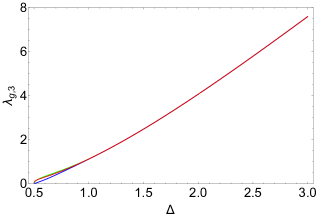
(a) $\lambda_{g,3}$ vs $\Delta$ overall.

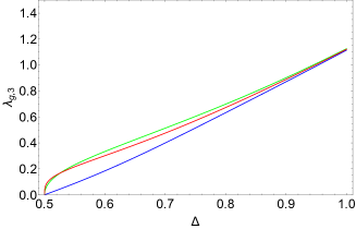
(b) $\lambda_{g,3}$ vs $\Delta$ zoomed

Figure 1: (a) $\lambda_{g,3}$ vs $\Delta$: Green, blue and red colored curves for $\lambda_{g,3}$ are obtained by letting $d_{N}=0$, with $N=30,31,32$ respectively. There are three branches in $1/2<\Delta<1$. And such brances merge for $\Delta\geq 1$. (b) Zoom in of figure (a) for the regime $1/2<\Delta<1$.

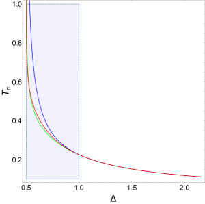
(a) $T_{c}$ vs $\Delta$ in $AdS_{4}$

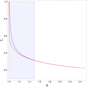
(b) $T_{c}$ vs $\Delta$ in $AdS_{5}$

Figure 2: (a) Shaded area should be eliminated due to the non-uniqueness of eigenvalues $\lambda_{g,3}$ shown in (a,b) at Fig. 1. This naturally elliminates $\Delta=1/2$ where $T_{c}$ diverges. We have set $g=\rho=1$. (b) Similarly, shaded area at $1\leq\Delta<3/2$ should be eliminated in $AdS_{5}$ due to the non-uniqueness of eigenvalues $\lambda_{g,4}$. This naturally elliminates $\Delta=1$ where $T_{c}$ diverges. There are two branches in $AdS_{5}$ unlike $AdS_{4}$.

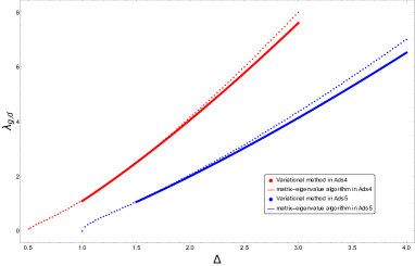
(a) $\lambda_{g,d}$ vs $\Delta$ for d=3,4

Figure 3: $\lambda_{g,d}$ vs $\Delta$: red line for $\lambda_{g,3}$ and blue line for $\lambda_{g,4}$. The results of variational method in ref. Siop2010 is denoted by red and blue dotted lines for AdS₄ and AdS₅ respectively.

The authors of ref.Siop2010 got $\lambda_{g,3}$’s by using variational method using the fact that the eigenvalue $\lambda_{g,3}$ minimizes the expression

$$\lambda_{g,3}^{2}=\frac{\int_{0}^{1}dz\;z^{2\Delta-2}\left((1-z^{3})\left[F^{{}^{\prime}}(z)\right]^{2}+\Delta^{2}z\left[F(z)\right]^{2}\right)}{\int_{0}^{1}dz\;z^{2\Delta-2}\frac{1-z}{1+z+z^{2}}\left[F(z)\right]^{2}}.$$ (40)

for $\Delta>1/2$. The integral does not converge at $\Delta=1/2$ because of $\ln(z)$. The trial function used is $F(z)=1-\alpha z^{2}$ where $\alpha$ is the variational parameter. Their result is given by the red dotted line in Fig. 3. While the variational method tells us that there are numerical values of $\lambda_{g,3}$ for $1/2<\Delta<1$, our method tells us that this region does not allow well defined value of $\lambda_{g,3}$, hence $T_{c}$ is not defined there.

The critical temperature is given by $T_{c}=\frac{3}{4\pi}\sqrt{\frac{\rho}{\lambda_{3}}}$, so that it can be calculated by once $\lambda$ is given. Notice that $T_{c}$ is a monotonically decreasing function of $\Delta$.

Similar statements are true for AdS5: Depending on even-ness or odd-ness of $n$, there are two branches if $1<\Delta<1.5$. Two branches merge in $\Delta\geq 1.5$ for AdS5. For more detail, see section B.1.2.

4 The condensation near critical temperature

Substrituting Eq.(11) into Eq.(3), the field equation $\Phi$ becomes

$$\frac{d^{2}\Phi}{dz^{2}}=\frac{g^{2}\left<\mathcal{O}_{\Delta}\right>^{2}}{r_{h}^{2\Delta}}\frac{z^{2(\Delta-1)}F^{2}(z)}{1-z^{3}}\Phi,$$ (41)

where ${g\left<\mathcal{O}_{\Delta}\right>^{2}}/{r_{h}^{2\Delta}}$ is small because $T\approx T_{c}$. The above equation have the expansion around Eq.(9) with small correction Siop2010 :

$$\frac{\Phi}{r_{h}}=\lambda_{3}(1-z)+\frac{g^{2}\left<\mathcal{O}_{\Delta}\right>^{2}}{r_{h}^{2\Delta}}\chi_{1}(z)$$ (42)

We have $\chi_{1}(1)=\chi_{1}^{{}^{\prime}}(1)=0$ due to the boundary condition $\Phi(1)=0$. Taking the derivative of Eq.(42) twice with respect to $z$ and using the result in Eq.(41),

$$\chi_{1}^{{}^{\prime\prime}}=\frac{z^{2(\Delta-1)}F^{2}(z)}{1-z^{3}}\left\{\lambda_{3}(1-z)+\frac{g^{2}\left<\mathcal{O}_{\Delta}\right>^{2}}{r_{h}^{2\Delta}}\chi_{1}\right\}\approx\frac{\lambda_{3}z^{2(\Delta-1)}F^{2}(z)}{z^{2}+z+1}.$$ (43)

Integrating Eq.(43) gives us

$$\chi_{1}^{{}^{\prime}}(0)=-\lambda_{3}\mathcal{C}_{3}\quad\hbox{ for }\mathcal{C}_{3}=\int_{0}^{1}dz\;\frac{z^{2(\Delta-1)}F^{2}(z)}{z^{2}+z+1}.$$ (44)

Eq.(11) with Eq.(14) shows

$$F(z)=(z^{2}+z+1)^{-\lambda_{g,3}/\sqrt{3}}y(z)\approx\left(z^{2}+z+1\right)^{-\frac{\lambda_{g,3}}{\sqrt{3}}}\sum_{n=0}^{15}d_{n}z^{n}.$$ (45)

Here, we ignore $d_{n}z^{n}$ terms if $n\geq 16$ because $0<|d_{n}|\ll 1$ numerically and $y(z)$ converges for $0\leq z\leq 1$.

We can calculate the numerical value of $\sqrt{1/\mathcal{C}_{3}}$ by putting Eq.(35) and Eq.(14) into eq.(44) and eq.(45). We calculated 102 different values of $\sqrt{1/\mathcal{C}_{3}}$’s at various $\Delta$, which is drawn as dots in Fig. 4. Then we tried to find an approximate fitting function. The result is given as follows,

$$\sqrt{\frac{1}{\mathcal{C}_{3}}}\approx\frac{\Delta^{6}+120\Delta^{1.5}}{84}$$ (46)

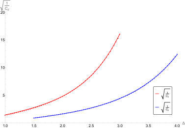
Figure 4: (a) $\sqrt{1/\mathcal{C}_{3}}$ data by eq.(44) and eq.(45) with eq.(35), as functions of $\Delta$. Red colored curve is the plot of eq.(46). (b) $\sqrt{1/\mathcal{C}_{4}}$ data by eq.(187) and eq.(188) with eq.(181), as functions of $\Delta$. Blue colored curve is the plot of eq.(189).

Fig. 4 shows how the data fits by above formula. From the Eq.(42) and Eq.(4), we have

$$\frac{\rho}{r_{h}^{2}}=\lambda_{3}\left(1+\frac{\mathcal{C}_{3}g^{2}\left<\mathcal{O}_{\Delta}\right>^{2}}{r_{h}^{2\Delta}}\right)$$ (47)

Putting $T=\frac{3}{4\pi}r_{h}$ with $\lambda_{3}=\frac{\rho}{r_{c}^{2}}$ into Eq.(47), we obtain the condensate near $T_{c}$:

$$g\frac{\left<\mathcal{O}_{\Delta}\right>}{T_{c}^{\Delta}}\approx\mathcal{M}_{3}\;\sqrt{1-\frac{T}{T_{c}}}\quad\hbox{ for }\mathcal{M}_{3}=\left(\frac{4\pi}{3}\right)^{\Delta}\sqrt{\frac{2}{\mathcal{C}_{3}}}$$ (48)

In ref. Siop2010 it was argued that $\lim_{\Delta\rightarrow d}\mathcal{C}_{d}=0$, which would lead to the divergence of the condensation in eq. (44). However, our result shows that $\lim_{\Delta\rightarrow d}\mathcal{C}_{d}=finite$ so that eq. (44) is finite, which can be confirmed in the FIG. 5. The condensate is an increasing function of the $\Delta$ but it decreases with increasing $T$.

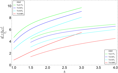
Figure 5: ${g^{\frac{1}{\Delta}}\langle O_{\Delta}\rangle^{\frac{1}{\Delta}}}/{T_{c}}$ vs $\Delta$ for a few $T$’s near $T_{c}$. Sold curves are for AdS₄ and dotted ones are for AdS₅.

As we substitute eq. (7) into eq. (48), we obtain

$$g\frac{\left<\mathcal{O}_{\Delta}\right>}{(g\rho)^{\frac{\Delta}{2}}}\approx\lambda_{g,3}^{-\frac{\Delta}{2}}\sqrt{\frac{2}{\mathcal{C}_{3}}}\;\sqrt{1-\frac{T}{T_{c}}}$$ (49)

The square root temperature dependence is typical of a mean field theory Hart2008 ; Herzog:2010vz ; Siop2010 . Our main interest here is the $\Delta$ dependence of the ${\cal M}_{3}$, especially the singular dependence through ${\cal C}_{3}$ whose values for some particular value of $\Delta$ was obtained before: for $\Delta=1$, we have $\mathcal{M}_{3}=8.53$ which is in good agreement with the ${\mathcal{M}}_{3}=9.3$ Hart2008 . For $\Delta=2$, we have ${\mathcal{M}}_{3}=119.17$ which roughly agrees with the results ${\mathcal{M}}_{3}=119$ of ref. Jing2020 and ${\mathcal{M}}_{3}=144$ of ref. Hart2008 . We obtained the approximate results for general $\mathcal{C}_{d}$. See eq.(46) and Eq.(189) in the appendix. For large $\Delta$, $\mathcal{C}_{d}\sim\Delta^{-(d+9)}$. We conclude that we do not have a singular dependence of the condensation anywhere for the s-wave holographic superconductivity, which is different from the result of ref. Siop2010 . See the FIG. 5.

5 The AC Conductivity for $\Delta=1,2$ in 2+1

The Maxwell equation for the planar wave solution with zero spatial momentum and frequency $\omega$ is

$$r_{+}^{2}(1-z^{3})^{2}\frac{d^{2}A_{x}}{dz^{2}}-3r_{+}^{2}z^{2}(1-z^{3})\frac{dA_{x}}{dz}+\left(\omega^{2}-V(z)\right)A_{x}=0,$$ (50)

where $A_{x}$ is the perturbing electromagnetic potential and

$$V(z)=\frac{g^{2}\left<\mathcal{O}_{\Delta}\right>^{2}}{r_{+}^{2\Delta-2}}(1-z^{3})z^{2\Delta-2}F(z)^{2},$$

with $F$ defined as before. To request the ingoing boundary conditions at the horizon, $z=1$, we introduce $G(z)$ by $A_{x}(z)=(1-z)^{-\frac{i}{3}\hat{\omega}}G(z)$ where $\hat{\omega}=\omega/r_{+}$. Then the wave equation Eq.(50) reads

$$(1-z^{3})\frac{d^{2}G}{dz^{2}}+\left(-3z^{2}+\frac{2i\hat{\omega}}{3}(1+z+z^{2})\right)\frac{dG}{dz}$$ (51)

$$+\left(\frac{(2+z)(4+z+z^{2})}{9(1+z+z^{2})}\hat{\omega}^{2}+\frac{i\hat{\omega}}{3}(1+2z)-\frac{g^{2}\left<\mathcal{O}_{\Delta}\right>^{2}}{r_{+}^{2\Delta}}z^{2\Delta-2}F^{2}(z)\right)G=0$$

If the asymptotic behaviour of the Maxwell field at large $r$ is given by

$$A_{x}=A_{x}^{(0)}+\frac{A_{x}^{(1)}}{r}+\cdots,$$ (52)

then the conductivity is given by

$$\sigma(\omega)=\frac{1}{i\omega}\frac{A_{x}^{(1)}}{A_{x}^{(0)}}=\frac{1}{i\hat{\omega}}\frac{\frac{dG(0)}{dz}+\frac{i\hat{\omega}}{3}G(0)}{G(0)}.$$ (53)

Near the $T=0$, the equation Eq.(51) is simplied to

$$\frac{d^{2}G}{dz^{2}}+\frac{2i\hat{\omega}}{3}\frac{dG}{dz}+\left(\frac{8}{9}\hat{\omega}^{2}+\frac{i\hat{\omega}}{3}-\frac{g^{2}\left<\mathcal{O}_{\Delta}\right>^{2}}{r_{+}^{2\Delta}}z^{2\Delta-2}F(z)^{2}\right)G=0.$$ (54)

For $\Delta=1$, $F(z)\approx 1$ so that the solution of Eq.(54) is

$$G(z)=\exp\left(iz\left(-\frac{\omega}{3}+\sqrt{\omega^{2}+\frac{i\omega}{3}-\frac{g^{2}\left<\mathcal{O}_{1}\right>^{2}}{r_{+}^{2}}}\right)\right)+R\;\exp\left(iz\left(-\frac{\omega}{3}-\sqrt{\omega^{2}+\frac{i\omega}{3}-\frac{g^{2}\left<\mathcal{O}_{1}\right>^{2}}{r_{+}^{2}}}\right)\right)$$

Here, $R$ is a constant called reflection coefficient. Taking the zero temperature limit $T\rightarrow 0$ is equivalent to sending the horizon to infinity. Then the in-falling boundary condition corresponds to $R=0$. Then it gives the conductivities,

$$\sigma(\omega)=\frac{g\left<\mathcal{O}_{1}\right>}{\omega}\sqrt{\left(1+\frac{ir_{+}}{3\omega}\right)\left(\frac{\omega}{g\left<\mathcal{O}_{1}\right>}\right)^{2}-1}.$$ (55)

Compare Figure 6(d)(a) with Figure 6(d)(c). Similary, for $\Delta=2$, we can obtain the conductivity given as follow,

$$\sigma(\omega)=\frac{3i\sqrt{g\left<\mathcal{O}_{2}\right>}}{\sqrt{2}\omega}\frac{\Gamma\left(0.24-\frac{4i}{9}\sqrt{P(\omega)}\right)}{\Gamma\left(-0.26-\frac{4i}{9}\sqrt{P(\omega)}\right)}\frac{\Gamma\left(1.26-\frac{4i}{9}\sqrt{P(\omega)}\right)}{\Gamma\left(0.76-\frac{4i}{9}\sqrt{P(\omega)}\right)}$$ (56)

where

$$P(\omega)=\frac{9}{8}\left(1+\frac{ir_{+}}{3\omega}\right)\left(\frac{\omega}{\sqrt{g\left<\mathcal{O}_{2}\right>}}\right)^{2}-1$$

This result fits the numerical data almost exactly as one can see in Figure 6(d)(b). And it is consistent with the result of ref. Horo2009 ; compare Figure 6(d)(b) with Figure 6(d)(d). For derivation of these results, see the appendix A.2.1.

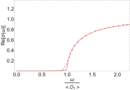
(a) $Re$$(\sigma(\omega))$ for $\Delta=1$.

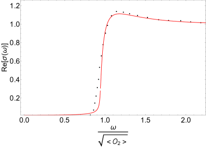
(b) $Re$$(\sigma(\omega))$ for $\Delta=2$.

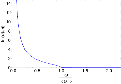
(c) $Im$$(\sigma(\omega))$ for $\Delta=1$.

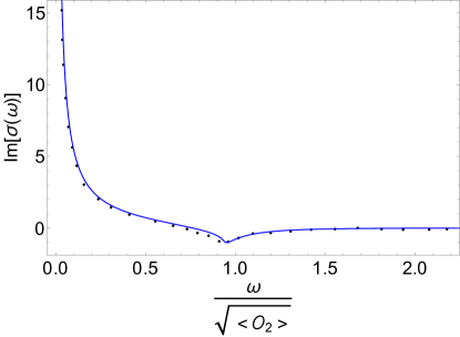
(d) $Im$$(\sigma(\omega))$ for $\Delta=2$.

Figure 6: Analytic results (real lines) vs numerical results(dotted lines). (a,b) Plots of $Re$$(\sigma(\omega))$ in Eq.(55) and Eq.(56). Dot points are numerical results in Fig. 3. of ref. Hart2008 . (c,d) Plots of $Im$$(\sigma(\omega))$. Dot points are from Fig. 4. of ref. Hart2008 . In all cases $T/T_{c}=0.1$.

.

To request the ingoing boundary conditions at the horizon, $z=1$, we introduce $H(z)$ by $A_{x}(z)=(1-z^{3})^{-\frac{i}{3}\hat{\omega}}H(z)$ where $\hat{\omega}=\omega/r_{+}$. Then the wave equation Eq.(50) reads

$$(1-z^{3})\frac{d^{2}H}{dz^{2}}-3\left(1-\frac{2i\hat{\omega}}{3}\right)z^{2}\frac{dH}{dz}$$ (57)

$$+\left(\frac{\hat{\omega}^{2}(1+z)(1+z^{2})}{1+z+z^{2}}+2i\hat{\omega}z-\frac{g^{2}\left<\mathcal{O}_{\Delta}\right>^{2}}{r_{+}^{2\Delta}}z^{2\Delta-2}F^{2}(z)\right)H=0$$

The boundary conditions at the horizon are Horo2014

$$H(1)=1,\quad\lim_{z\rightarrow 1}(1-z^{3})^{-\frac{i}{3}\hat{\omega}}H^{\prime}(z)=0.$$

To evaluate the conductivities at low frequency, it is enough to obtain $H(z)$ up to first order in $\omega$,

$$H(z)=H_{0}(z)+\omega H_{1}(z)+\mathcal{O}(\omega^{2}).$$ (58)

Inserting this into Eq.(57), $H_{0}(z)$ and $H_{1}(z)$ satisfy

$$(1-z^{3})H_{0}^{\prime\prime}-3z^{2}H_{0}^{\prime}-\Delta^{2}b^{2\Delta}z^{2\Delta-2}F(z)^{2}H_{0}=0,$$ (59)

$$(1-z^{3})H_{1}^{\prime\prime}-3z^{2}H_{1}^{\prime}-\Delta^{2}b^{2\Delta}z^{2\Delta-2}F(z)^{2}H_{1}=-2iz(zH_{0}^{\prime}+H_{0}).$$ (60)

where $b^{\Delta}=\frac{g\left<\mathcal{O}_{\Delta}\right>}{\Delta r_{+}^{\Delta}}$. Near the $T=0$ we can simplify two coupled equations Eq.(59) and Eq.(60) as

$$H_{0}^{\prime\prime}-\Delta^{2}b^{2\Delta}z^{2\Delta-2}H_{0} = 0,$$ (61)

$$H_{1}^{\prime\prime}-\Delta^{2}b^{2\Delta}z^{2\Delta-2}H_{1} = -2izH_{0}.$$ (62)

The conductivity is given by

$$\sigma(\omega)=\frac{1}{i\omega}\frac{A_{x}^{(1)}}{A_{x}^{(0)}}=\frac{1}{i\hat{\omega}}\frac{\frac{dH(0)}{dz}}{H(0)}.$$ (63)

The solution of Eq.(63) is given in Eq.(64). Here, $n_{s}$ is the coefficient of the pole in the imaginary part ${\rm Im}{\sigma(\omega)}\sim n_{s}/\omega$ as $\omega\rightarrow 0$. For derivation of these results, see the appendix A.2.1. For the $\Delta$ values other than 1 or 2, there is no analytic result available at this moment.

6 Discussion

One problem is that denef2009landscape ; Siop2010 ; siopsis2011holographic the critical temperature is divergent at the $\Delta=1/2$, which does not seems to make physical sense and it has not been understood as far as we know. This was also noticed as a problem Horo2009 but the reason for it has not been cleared yet.

In this paper, we consider the problem of divergence of the critical temperature at $\Delta=1/2$ by recalculating $T_{c}$ using Pincherle’s theoremLeav1990 to handle the Heun’s equation. We find that the region of $1/2\leq\Delta<1$ for AdS₄ does not have well defined critical temperature. Similar phenomena also occur in AdS5. We also computed the AC conductivity gap $\omega_{g}$ and in this same regime, it does not exist either. The situation is similar to the physics of the pseudo gap where Cooper pairs are formed but the phase alignment of the pairs are absent. In the future work, we will work out the same phenomena in other background and also for non s-wave situation, to confirmed the universality of the phenomena.

Appendices

Appendix A Holographic superconductors with AdS₄

The theory of holographic superconductors are much studied. Some of the relevant papers for the analytical techniques can be found, for example, in refs. cai2015introduction ; ge2010analytical ; gangopadhyay2012analytic ; pan2010general ; cai2011analytical ; jing2011holographic ; roychowdhury2012effect ; gangopadhyay2012analytics ; li2011analytical ; pan2011analytical ; zeng2011analytical ; flauger2011striped ; zhao2013notes ; liu2011holographic ; zhao2013holographic ; roychowdhury2013ads ; kanno2011note ; peng2011various ; pan2012analytical ; banerjee2013holographic ; yao2013analytical ; lu2014lifshitz ; sheykhi2016analytical ; ghorai2016higher ; sheykhi2016analyticals ; lai2015analytical ; liu2010dynamical ; erdmenger2013striped ; kuang2013building ; gangopadhyay2014holographic ; zhang2015holographic ; cai2011magnetic ; kim2013holographic ; yao2014holographic . After initial stage of the the model building Hart2008 ; Gubser:2008px where probe limit of the gravity background was used, full back reacted version Hartnoll:2016apf . Although there are a few differences in the zero temperature limit, the probe limit captures most of the physicsHoro2009 . Later on, physical observables of the superconductivity are numerically calculated Horo2009 as functions of the conformal weight ($\Delta$) of the Cooper pair operator. These include ${\mathcal{O}_{\Delta}}$. $T_{c},\langle{\mathcal{O}}_{\Delta}\rangle,\sigma({\omega}),\omega_{g},\omega_{i},n_{s},$ which are the critical temperature, the condensation of the Cooper pair operator, the AC conductivity, the gap in the AC conductivity, the resonance frequencies, and the density of the cooper pairs respectively.

Since the parametric dependences of observables are crutial in understanding the underlying physics, it would be nice to have an analytic expressions within the probe approximation, while it would be senseless to try to replace the fully back reacted numerical solution. Works in this direction had been initiated in Siop2010 ; siopsis2011holographic . In this paper, we reconsider the problem since many of the result could not be reproduced. We got the analytic results which also agree with the numerical results of the original paper Horo2009 . Since the details are rather long, we summarize our results here.

We also calculated the the Cooper pair condensation $\left<\mathcal{O}_{\Delta}\right>$ as an analytic function of $\Delta$, which is plotted in FIG. 7 where we compared our results (real colored lines) with those of ref. Horo2009 (a few red dotted data ) and Siop2010 (black broken line). Noticed that the condensation does not change much for a region around $\Delta=2$ and slowly increasing as $\Delta\to 3$. Our analytic formula reproduces the values of of ref. Horo2009 near $\Delta=2$ and gives a finite value of the condensation near $\Delta=3$ unlike ref. Siop2010 . Notice also that the condensation is almost independent of $T$ and $\Delta$ over $3/2<\Delta<3$ region. Interestingly, we will see that the flatness of the graph over the region $3/2<\Delta<3$ comes as a consequence of the remarkable cancellation of singularities of two functions at $\Delta=3/2$. Similar result holds in three spatial dimension as well as in two dimension.

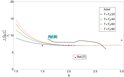
Figure 7: ${\left<\mathcal{O}_{\Delta}\right>^{\frac{1}{\Delta}}}/{T_{c}}$ vs $\Delta$ for $d=3$. Smooth colored lines are our results. Here, $T_{0}=\rho^{\frac{1}{2}}$ with $g=1$. For large $\Delta>3$, the graph does not saturate to a constant but increases slowly.

Our results for $T_{c}$ , $\left<\mathcal{O}_{\Delta}\right>/T_{c}^{\Delta}$ and $\left<\mathcal{O}_{\Delta}\right>$ for both near $T=T_{c}$ and $T=0$ are summarized in the Table 1 and 2.

AdSd+1	$\quad\;T_{c}\sim\left({g}{\rho}\right)^{1/(d-1)}$ for $\frac{d-1}{2}\leq\Delta\leq d$
$T\approx T_{c}$	$\left<\mathcal{O}_{\Delta}\right>\sim l^{-\Delta}g^{\gamma_{g}}\sqrt{1-\frac{T}{T_{c}}}$ for $\frac{d-1}{2}\leq\Delta\leq d$
$T\approx 0$	$\left<\mathcal{O}_{\Delta}\right>\sim l^{-\Delta}g^{\gamma_{g}}\left(\frac{T_{0}}{T}\right)^{\gamma_{1}}$ if $\frac{d-2}{2}<\Delta\ll\frac{d}{2}$
	$\left<\mathcal{O}_{\Delta}\right>\sim l^{-\Delta}g^{\gamma_{g}}\left(\ln\frac{T_{0}}{T}\right)^{\gamma_{2}}$ if $\Delta=\frac{d}{2}$
	$\left<\mathcal{O}_{\Delta}\right>\sim l^{-\Delta}g^{\gamma_{g}}$ if $\frac{d}{2}\ll\Delta\leq d$

Table 1: $T_{c}$ and $\left<\mathcal{O}_{\Delta}\right>$ near $T=T_{c}$ and $T=0$. Here, $\gamma_{1}=\frac{\Delta(d-2\Delta)}{(d-2+2\Delta)}$, $\gamma_{2}=\frac{\Delta}{2(d-1)}$ and $T_{0}=\left(g\rho\right)^{\frac{1}{d-1}}$ respectively, and $l={\rho}^{-\frac{1}{d-1}}$ is the distance scale given by the density $\rho$.

AdSd+1
$T\approx T_{c}$	$\left<X\right>\sim l^{d-1}\sqrt{1-\frac{T}{T_{c}}}$ for $\frac{d-1}{2}\leq\Delta\leq d$
$T\approx 0$	$\left<X\right>\sim l^{d-1}\left(\frac{T_{c}}{T}\right)^{\gamma_{1}}$ if $\frac{d-1}{2}\leq\Delta\ll\frac{d}{2}$
	$\left<X\right>\sim l^{d-1}\left(\ln\frac{T_{c}}{T}\right)^{\gamma_{2}}$ if $\Delta=\frac{d}{2}$
	$\left<X\right>\sim l^{d-1}$ if $\frac{d}{2}\ll\Delta\leq d$

Table 2: $\left<X\right>:=\frac{\left<\mathcal{O}_{\Delta}\right>}{T_{c}^{\Delta}}$ near $T=T_{c}$ and $T=0$.

The second quantity calculated is $\omega_{g}$, the gap in the optical (AC) conductivity. Notice that there is no solution for $\omega_{g}$ at $1/2<\Delta<1$; see appendix A.3.1. The co-incidence of this regime with that of non-existence of the critical temperature gives us a confidence in concluding the absence of the superconductivity in this regime. Our results for the $\omega_{g}$ is summarized in the Table 3, which are plotted in FIG. 8. The size of the gap is defined by $\omega_{g}=\sqrt{V_{\mbox{max}}}$ Horo2009 ; one should notice that ref. Horo2009 and ref. Horo2011 use slightly different definition of $\omega_{g}$.

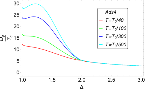
Figure 8: $\omega_{g}/T_{c}$ vs $\Delta$ for $d=3$. Here, $T_{0}=(g\rho)^{\frac{1}{2}}$. For $\Delta>3$, it decreases slowly.

$\omega_{g}/T_{c}=c_{1}X^{\Delta}\left(\frac{T_{c}}{T}\right)^{\Delta-1}$, for $1\leq\Delta\ll\frac{3}{2}$, $c_{1}=\left(\frac{3z_{0}}{4\pi}\right)^{\Delta-1}\left(1-\left(\frac{\Delta}{3-\Delta}z_{0}^{3/2-\Delta}\right)^{2}\right)$
$\omega_{g}/T_{c}=c_{2}\frac{{X^{3/2}\left(\frac{T_{c}}{T}\right)^{1/2}}}{\ln\left(X\frac{T_{c}}{T}\right)}$, for $\Delta=\frac{3}{2}$, ${\scriptsize c_{2}=\frac{7}{10}}$
$\omega_{g}/T_{c}=c_{3}X^{3-\Delta}\left(\frac{T_{c}}{T}\right)^{2-\Delta}$ for $\frac{3}{2}\ll\Delta<2$, ${\scriptsize c_{3}=c_{30}\left[1-\left(\frac{\Delta}{3-\Delta}z_{0}^{\Delta-3/2}\right)^{2}\right]}$
$\omega_{g}/T_{c}=c_{4}X$ for $2\leq\Delta\leq 3$, ${\scriptsize c_{4}=\frac{1.1}{\mbox{Li}(\Delta^{1.2})}}$

Table 3: $\omega_{g}/T_{c}$ as function of ${\scriptsize X=\frac{g^{1/\Delta}\left<\mathcal{O}_{\Delta}\right>^{1/\Delta}}{T_{c}}}$ near $T\approx 0$. $c_{30}=\frac{\sqrt{\pi}\left({3z_{0}}/{4\pi}\right)^{2-\Delta}\Gamma\left(\frac{3+\Delta}{2+\Delta}\right)\csc\left(\frac{\pi}{2\Delta}\right)}{\Delta^{3/\Delta}\Gamma\left(\frac{2}{\Delta}\right)\Gamma\left(\frac{3}{2\Delta}\right)\Gamma\left(1+\frac{1}{\Delta}\right)}$.

Notice that $\omega_{g}/T_{c}$ has the slightly decreasing tendency as a function of $\Delta$ instead of the slowly increasing behavior of ref. Horo2009 . So there is a small mismatch between the two.

The third quantity we calculated is the superfluid density $n_{s}$, which appears as the residue of the pole in the imaginary part of the optical conductivity at $\omega=0$. We obtained it as an analytic function of $\Delta$ given below,

$$\frac{n_{s}}{T_{c}}=\frac{2\pi\Delta\csc\left(\frac{\pi}{2\Delta}\right)}{(2\Delta)^{1/\Delta}\left(\Gamma\left(\frac{1}{2\Delta}\right)\right)^{2}}\frac{g^{1/\Delta}\left<\mathcal{O}_{\Delta}\right>^{1/\Delta}}{T_{c}},$$ (64)

which is plotted in FIG. 9. By plotting our result, we find that it agrees with the numerical result of ref. Horo2009 for all the data points given there: See FIG. 9.

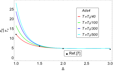
Figure 9: $n_{s}/T_{c}$ vs $\Delta$ for $d=3$. Colored real lines are plots of our analytic results while the black points are numerical data of ref. Horo2009 . Notice that it is almost independent of $T$ and $\Delta$ over the region $2\leq\Delta\leq 3$.

It has been believed that $\left<\mathcal{O}_{\Delta}\right>^{1/\Delta}$, $T_{c}$ and $\omega_{g}$ are the same quantity up to a numerical factor. This may the case if we look at them for a given $\Delta$. However, as functions of $\Delta$, they are all different ones, as we can see in figure 10. The identification of these observables partially make sense in the relatively large $\Delta>2$ regime. It is also interesting to notice that $\frac{\omega_{g}}{\left<\mathcal{O}_{\Delta}\right>^{1/\Delta}}$ is the maximum at $\Delta=3/2$ as one can see in figure 10(f).

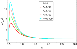
(a) $\left<\mathcal{O}_{\Delta}\right>^{1/\Delta}$ vs $\Delta$.

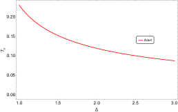
(b) $T_{c}$ vs $\Delta$.

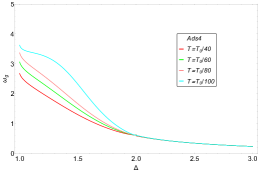
(c) $\omega_{g}$ vs $\Delta$.

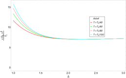
(d) $\frac{\left<\mathcal{O}_{\Delta}\right>^{1/\Delta}}{T_{c}}$ vs $\Delta$.

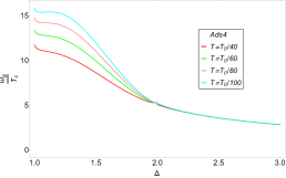
(e) $\frac{\omega_{g}}{T_{c}}$ vs $\Delta$.

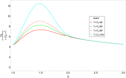
(f) $\frac{\omega_{g}}{\left<\mathcal{O}_{\Delta}\right>^{1/\Delta}}$ vs $\Delta$.

Figure 10: (a-f) Low temperature behavior of observables we calculated in this paper. Here, we set $d=3$ and $g=\rho=1$.

A.1 Condensate near the zero temperature

In general, Eq.(3) shows us that $F(z)$ in Eq. (11) does not converge at $z=1$. But the previous section 3.1 says that it is converged at the horizon with specific value of $\left<\mathcal{O}_{\Delta}\right>$. Its means whether we can find eigenvalue of it at $z=1$ or not simply, satisfied for $F(1)<\infty$. Unlike $T\approx T_{c}$ case, it is really hard to find the eigenvalue $\left<\mathcal{O}_{\Delta}\right>$ at $T\approx 0$. Because Eq.(3) are nonlinear coupled equations: $\Phi(z)$ cannot be described in a linear equation any longer unlike $T\approx T_{c}$ case. Instead, we use the perturbation theory for the eigenvalue at $T\approx 0$.

We can simplify Eq.(3) in $T\rightarrow 0$ limit by defining

$$\Psi(z)=({\left<\mathcal{O}_{\Delta}\right>}/{\sqrt{2}r_{h}^{\Delta}})z^{\Delta}F(z).$$ (65)

The equations of motion for F near the zero temperature becomes

$$\frac{d^{2}F}{dz^{2}}-\frac{2\Delta+1-d}{z}\frac{dF}{dz}+\frac{g^{2}\Phi^{2}}{r_{h}^{2}}F=0,$$ (66)

$$\frac{d^{2}\Phi}{dz^{2}}-\frac{d-3}{z}\frac{d\Phi}{dz}-\frac{g^{2}\left<\mathcal{O}_{\Delta}\right>^{2}}{r_{h}^{2\Delta}}z^{2(\Delta-1)}F^{2}\Phi=0.$$

The boundary conditions (BC) we should use are

$$\frac{d\Phi(0)}{dz^{d-2}}=-\frac{\rho}{r_{h}^{d-2}},\quad F(0)=1,$$ (67)

and

$$\Phi(1)=0,\quad 3\frac{dF(1)}{dz}+\Delta^{2}F(1)=0.$$ (68)

The latter is the horizon regularity conditions at $z=1$, and from (A.39) one can derive $F^{\prime}(0)=0$.

We use $X$ to denote $g^{\frac{1}{\Delta}}\frac{\left<\mathcal{O}_{\Delta}\right>^{\frac{1}{\Delta}}}{T_{c}}$ which appears often. Then, $X$ satisfies

$$X^{2(d-1)}=G_{d}^{2(d-1)}\left(\alpha_{d}+\beta_{d}\tau_{d}^{d-2\Delta}X^{d-2\Delta}\right)$$ (69)

$$\hbox{where }\quad G_{d} = \frac{4\pi\Delta^{1/\Delta}}{d}\left(\frac{-2^{1+\nu}\lambda_{g,d}}{\Gamma(-\nu)}\right)^{\frac{1}{d-1}}$$ (70)

$$\alpha_{d} = -\frac{\sqrt{\pi}\Gamma\left(\frac{d-2\Delta}{2\Delta}\right)\Gamma\left(\frac{1}{\Delta}\right)\Gamma\left(\frac{d-1}{\Delta}\right)}{8\Delta^{2}\Gamma\left(\frac{d+\Delta}{2\Delta}\right)}$$ (71)

$$\beta_{d} = \frac{\nu\pi(d-\Delta)^{2}\csc(\nu\pi)}{2\Delta^{3}\left(d-2\Delta\right)}.$$ (72)

with $\nu=\frac{d-2}{2\Delta}$ and $\tau_{d}=\frac{d}{4\pi\Delta^{1/\Delta}}\frac{T_{c}}{T}$. For derivation of this result, see the appendix A.1. We can get the solution of Eq.(102) according to the regimes of $\Delta$:
$X=G_{d}^{\frac{2(d-1)}{d-2+2\Delta}}\beta_{d}^{\frac{1}{d-2+2\Delta}}\tau_{d}^{\frac{d-2\Delta}{d-2+2\Delta}}$ for $(d-2)/2<\Delta\ll d/2$:
$X=G_{d}\;\alpha_{d}^{\frac{1}{2(d-1)}}$ for $d/2\ll\Delta<d$. Especially, for $\Delta=\frac{d}{2}$

$$X^{2(d-1)}=G_{d}^{2(d-1)}\left(\rho_{d}+\sigma_{d}\ln(\tau_{d}X)\right)$$ (73)

where $\rho_{d}=\frac{\sigma_{d}}{d}\left(5-\frac{2}{d-2}-\pi\cot\left(\frac{2\pi}{d}\right)-2\psi\left(\frac{2}{d}\right)-\log(4)\right)$ and $\sigma_{d}=\frac{\pi(d-2)\csc\left(\frac{2\pi}{d}\right)}{d^{2}}$. Here, $\psi\left(z\right)$ is the digamma function. Details are available in appendix A.1.2 and B.2.2. Numerical results tell us that $\rho_{3}\approx 0.8$, $\rho_{4}\approx 0.64$ and $\sigma_{3}\approx 0.4\approx\sigma_{4}$. Therefore, eq.(73) becomes

$$X \approx 6.76\left(1+0.45\ln\left(\frac{T_{c}}{T}\right)\right)^{1/4}\;\;\;\mbox{for AdS${}_{4}$}$$

$$X \approx 4.9\left(1+0.57\ln\left(\frac{T_{c}}{T}\right)\right)^{1/6}\;\;\;\mbox{for AdS${}_{5}$}.$$ (74)

We can first test our result with known results: For $\Delta=1$ and $T=0.1T_{c}$, our analytic expression with $g=1$ gives ${\left<\mathcal{O}_{1}\right>}/{T_{c}}\approx 12.65$, which is comparable to the numerical result 10.8 of ref. Hart2008 . Our result, however, is different from that of ref. Siop2010 except at $\Delta=1$.

It is important to notice that the temperature dependence of the condensation $X=g^{\frac{1}{\Delta}}\frac{\left<\mathcal{O}_{\Delta}\right>^{\frac{1}{\Delta}}}{T_{c}}$ is very different depending on the regime of $\Delta$. It diverges as $T\to 0$ for $\Delta<\frac{d}{2}$, but it has little dependence on $T$ in $d/2<\Delta<d$. These results explains the numerical features of ref. Hart2008 .

Notice that there are presence of singularities at $\Delta=d/2$ in both $\alpha_{d}$ and $\beta_{d}$. Surprisingly, however, it turns out that there is no singularity in $X$. To understand this, notice that the behaviors of $\alpha_{d}$ near $\Delta=d/2$ is

$$\lim_{\Delta\rightarrow d/2}\alpha_{d} = \frac{(d-2)\pi\csc\left(\frac{2\pi}{d}\right)}{2d^{2}}\frac{1}{\Delta-d/2},$$ (75)

which is exactly the same as the behavior of $-\beta_{d}$ near $\Delta=d/2$. Therefore, the singularity of $X$ of eq.(102) disappears because at $\Delta=d/2$, $X^{d-2\Delta}=1$ and $\alpha_{d}+\beta_{d}$ is finite. Such cancellation of two singularities was rather unexpected.

In ref. Horo2009 , it was numerically noticed that $X$ is almost constant over the region $d/2<\Delta<d$. To understand this phenomena, we plot $\alpha_{3}$, $\beta_{3}$ and $G_{3}$ as function of $\Delta$ in the FIG. 11.

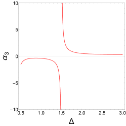
(a) $\alpha_{3}$ vs $\Delta$

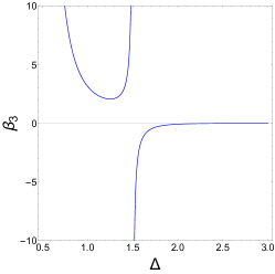
(b) $\beta_{3}$ vs $\Delta$

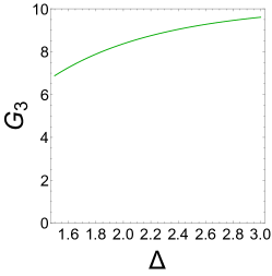
(c) $G_{3}$ vs $\Delta$

Figure 11: Plots of $\alpha_{3}$, $\beta_{3}$ and $G_{3}$ in eq.(103) over $1/2<\Delta<3$.

In fact, one can show that for $\Delta\gg\frac{3}{2}$,

$$\alpha_{d}=\frac{\Delta}{4(d-1)d}+\frac{1-3\gamma_{E}-\psi\left({1}/{2}\right)}{8(d-1)}+\cdots,$$ (76)

so that for $d=3$, $\alpha_{3}=\frac{\Delta}{24}+0.077$. Notice that $\alpha_{d}$ is flat over the relevant regime because the linear term grows with tiny slope. $\beta_{3}$, after vanishing at $\Delta=3$, saturate to 0 rapidly like $\sim-1/(4\Delta^{2})$. In addition, $G_{3}$ moves slowly in the FIG. 11. All these collaborate with the cancellation of the singularity at $\Delta=3/2$, to make the flatness of $X$ in $\Delta$ in the regime. Completely parallel reasoning works for $d=4$. It would be very interesting to see if this is only for s-wave case or it continue to be so for $p$- and $d$-wave case as well. We will leave this as a future work.

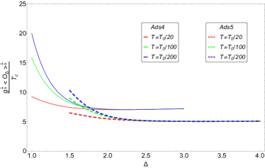
Figure 12: $g^{\frac{1}{\Delta}}\frac{\left<\mathcal{O}_{\Delta}\right>^{\frac{1}{\Delta}}}{T_{c}}$ vs $\Delta$ near $T=0$. Here, $T_{0}=(g\rho)^{\frac{1}{d-1}}$. Notice the flatness and the $T$-independence over $\frac{d}{2}<\Delta<d$.

Fig. 12 is the plot of the results given in Eq.(102) for $d=3,4$. The solid lines are for $d=3$, and the dashed lines are for $d=4$. $g^{\frac{1}{\Delta}}\frac{\left<\mathcal{O}_{\Delta}\right>^{\frac{1}{\Delta}}}{T_{c}}$ is $\sim 7$ at $3/2<\Delta<3$ for Ads₄, and $\sim 5$ at $2<\Delta<4$ for AdS₅. These are in good agreement with numerical results of ref. Horo2009 .

A remark is in order to explain why analytic formulae in $G_{d}$, $\alpha_{d}$ and $\beta_{d}$ were possible in spite of the fact that the differential equations in the black hole background are not of hypergeometric type, as we can see from Eq.(3). The simplification happens near $T=0$, where the higher order singularity at the horizon disappears as we can see from Eq.(A.1): there is only one regular singularity at $z=0$ and the order of the singularity is independent of $d$ so that the differential equations reduces to hypergeometric type. Details are available in appendix A.1.1, A.1.2, B.2.1 and B.2.2.

We use $Y$ to denote $g^{\frac{1}{\Delta}}\frac{\left<\mathcal{O}_{\Delta}\right>^{\frac{1}{\Delta}}}{T_{0}}$ which appears often. Here, $T_{0}=(g\rho)^{\frac{1}{d-1}}$. Then, $Y$ satisfies

$$Y^{2(d-1)}=\widetilde{G_{d}}^{2(d-1)}\left(\alpha_{d}+\beta_{d}\widetilde{\tau_{d}}^{d-2\Delta}Y^{d-2\Delta}\right)$$ (77)

$$\hbox{where }\quad\widetilde{G_{d}} = \Delta^{1/\Delta}\left(\frac{-2^{1+\nu}}{\Gamma(-\nu)}\right)^{\frac{1}{d-1}}$$ (78)

$$\widetilde{\tau_{d}} = \frac{d}{4\pi\Delta^{1/\Delta}}\frac{T_{0}}{T}.$$ (79)

For derivation of this result, see the appendix A.1.3 $\&$ B.2.3. Fig. 13 is the plot of the results given in Eq.(77) for $d=3,4$. We emphasize that although there is no $T_{c}$ in $\frac{d-2}{2}<\Delta<\frac{d-1}{2}$, there is well defined condensation in this regime.

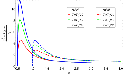
Figure 13: $g^{\frac{1}{\Delta}}\frac{\left<\mathcal{O}_{\Delta}\right>^{\frac{1}{\Delta}}}{T_{0}}$ vs $\Delta$ near $T=0$. Notice again the flatness and the $T$-independence over $\frac{d}{2}<\Delta<d$.

A.1.1 Analytic calculation of $g^{\frac{1}{\Delta}}\frac{\left<\mathcal{O}_{\Delta}\right>^{\frac{1}{\Delta}}}{T_{c}}$ at $1\leq\Delta<3$

The Hawking temperature shows $r_{h}\rightarrow 0$ as $T\rightarrow 0$. We can say $z=r_{h}/r\rightarrow 0$ at $r\gg r_{h}$ and the dominant contribution comes from the neighborhood of the boundary $z=0$. So near the $T=0$ we can simplify two coupled equations Eq.(3) and Eq.(3) with Eq.(11) by letting $z\rightarrow 0$:

$$\frac{d^{2}F}{dz^{2}}+\frac{2(\Delta-1)}{z}\frac{dF}{dz}+\frac{g^{2}\Phi^{2}}{r_{h}^{2}}F=0$$ (80a)

$$\frac{d^{2}\Phi}{dz^{2}}-\frac{g^{2}\left<\mathcal{O}_{\Delta}\right>^{2}}{r_{h}^{2\Delta}}z^{2(\Delta-1)}F^{2}\Phi=0.$$ (80b)

We use a boundary condition at the horizon, and Eq.(3) with Eq.(11) is rewritten as

$$-\frac{d^{2}F}{dz^{2}}+\left(\frac{2+z^{3}}{z(1-z^{3})}-\frac{2\Delta}{z}\right)\frac{dF}{dz}+\left(\frac{\Delta^{2}z}{1-z^{3}}-\frac{g^{2}\Phi^{2}}{r_{h}^{2}(1-z^{3})^{2}}\right)F=0$$ (81)

and it provides us the following boundary condition at the horizon with Eq.(3), $\Phi(1)=0$ and $\Psi(1)<\infty$:

$$3F^{{}^{\prime}}(1)+\Delta^{2}F(1)=0.$$ (82)

By multiplying $z$ to the eq. (81) and then taking the limit of $z\to 0$, we get $F^{{}^{\prime}}(0)=0$. Note that $F(0)=1$ should be considered as the normalization condition of $\langle{\cal O}_{\Delta}\rangle$ rather than as a boundary condition. Also for canonical system, we regard the $\Phi^{\prime}(0)=-\frac{\rho}{r_{h}}$ as BC and $\Phi(0)=\mu$ is not a BC but a value that should be determined by $\rho$ from the horizon regularity condition $\Phi(1)=0$. In Grand canonical system $\Phi(0)=\mu$ is the boundary condition and $\rho$ should be determined from it by the $\Phi(1)=0$. Here we consider $\rho$ as the given parameter.

If we introduce $b$ by $\hbox{ for }b^{\Delta}=\frac{g\left<\mathcal{O}_{\Delta}\right>}{\Delta r_{h}^{\Delta}}$, the solution to Eq.(80b) for $\Phi$ with $F\approx 1$ is

$$\Phi(z) = \mathcal{A}r_{h}\sqrt{bz}K_{\frac{1}{2\Delta}}\left(b^{\Delta}z^{\Delta}\right)\quad$$ (83)

At the horizon $\Phi(1)\varpropto\exp(-b^{\Delta})\rightarrow 0$ because $b\rightarrow\infty$ as $r_{h}\rightarrow 0$ ($T\rightarrow 0$), which takes care the boundary condition $\Phi(1)=0$. Substituting Eq.(83) into Eq.(80a), $F$ becomes

$$\frac{d^{2}F}{dz^{2}}+\frac{2(\Delta-1)}{z}\frac{dF}{dz}+g^{2}b\mathcal{A}^{2}z\left(K_{\frac{1}{2\Delta}}\left(b^{\Delta}z^{\Delta}\right)\right)^{2}F=0.$$ (84)

$F(z)$ can be obtained iteratively starting from $F=1$. The result is

$$F(z)=1-g^{2}b\mathcal{A}^{2}\int_{0}^{z}d\acute{z}\;\acute{z}^{2(1-\Delta)}\int_{0}^{\acute{z}}d{\ooalign{\kern 1.00006pt\hbox{\raise 0.0pt\hbox{\'{}}}\kern-2.5pt\hbox{\raise 0.0pt\hbox{\'{}}}\cr\hbox{z}\crcr}}\;{\ooalign{\kern 1.00006pt\hbox{\raise 0.0pt\hbox{\'{}}}\kern-2.5pt\hbox{\raise 0.0pt\hbox{\'{}}}\cr\hbox{z}\crcr}}^{2\Delta-1}\left(K_{\frac{1}{2\Delta}}\left(b^{\Delta}{\ooalign{\kern 1.00006pt\hbox{\raise 0.0pt\hbox{\'{}}}\kern-2.5pt\hbox{\raise 0.0pt\hbox{\'{}}}\cr\hbox{z}\crcr}}^{\Delta}\right)\right)^{2}$$ (85a)

$$F^{{}^{\prime}}(z)=-g^{2}b\mathcal{A}^{2}z^{2(1-\Delta)}\int_{0}^{z}d{\ooalign{\kern 1.00006pt\hbox{\raise 0.0pt\hbox{\'{}}}\kern-2.5pt\hbox{\raise 0.0pt\hbox{\'{}}}\cr\hbox{z}\crcr}}\;{\ooalign{\kern 1.00006pt\hbox{\raise 0.0pt\hbox{\'{}}}\kern-2.5pt\hbox{\raise 0.0pt\hbox{\'{}}}\cr\hbox{z}\crcr}}^{2\Delta-1}\left(K_{\frac{1}{2\Delta}}\left(b^{\Delta}{\ooalign{\kern 1.00006pt\hbox{\raise 0.0pt\hbox{\'{}}}\kern-2.5pt\hbox{\raise 0.0pt\hbox{\'{}}}\cr\hbox{z}\crcr}}^{\Delta}\right)\right)^{2}$$ (85b)

with the boundary condition $F^{{}^{\prime}}(0)=0$ and normalized $F(0)=1$. Applying the boundary condition Eq.(82) into Eq.(85a) and Eq.(85b), we obtain

$$g^{2}\mathcal{A}^{2}=\frac{\Delta^{2}b^{2}}{3F_{\Delta}^{{}^{\prime}}(b)+\Delta^{2}F_{\Delta}(b)}$$ (86)

where

$$F_{\Delta}(b)=\int_{0}^{b}dz\;z^{2-2\Delta}\int_{0}^{z}d\tilde{z}\;\tilde{z}^{2\Delta-1}\left(K_{\frac{1}{2\Delta}}\left(\tilde{z}^{\Delta}\right)\right)^{2}$$ (87a)

$$F_{\Delta}^{{}^{\prime}}(b)=b^{3-2\Delta}\int_{0}^{b}dz\;z^{2\Delta-1}\left(K_{\frac{1}{2\Delta}}\left(z^{\Delta}\right)\right)^{2}.$$ (87b)

With $x=z^{\Delta}$, Eq.(87b) is simplified as

$$F_{\Delta}^{{}^{\prime}}(b)=\frac{b^{3-2\Delta}}{\Delta}\int_{0}^{b^{\Delta}}dx\;x\left(K_{\frac{1}{2\Delta}}\left(x\right)\right)^{2}\approx\frac{b^{3-2\Delta}}{\Delta}\int_{0}^{\infty}dx\;x\left(K_{\frac{1}{2\Delta}}\left(x\right)\right)^{2}.$$ (88)

There is the integral formula GRAD1980 :

$$\int_{0}^{\infty}dx\;x^{-\lambda}K_{\mu}\left(x\right)K_{\nu}\left(x\right)=\frac{2^{-2-\lambda}}{\Gamma(1-\lambda)}\Gamma\left(\frac{1-\lambda+\mu+\nu}{2}\right)\Gamma\left(\frac{1-\lambda-\mu+\nu}{2}\right)\Gamma\left(\frac{1-\lambda+\mu-\nu}{2}\right)\Gamma\left(\frac{1-\lambda-\mu-\nu}{2}\right)$$ (89)

where $Re\;\lambda<1-|Re\;\mu|-|Re\;\nu|$. Using Eq.(89), Eq.(88) becomes

$$F_{\Delta}^{{}^{\prime}}(b)=\frac{\pi}{4\Delta^{2}}\csc{\left(\frac{\pi}{2\Delta}\right)}b^{3-2\Delta}$$ (90)

Letting $x=\tilde{z}^{\Delta}$, Eq.(87a) is simplified as

$$F_{\Delta}(b)=\frac{1}{\Delta}\int_{0}^{b}dz\;z^{2-2\Delta}\int_{0}^{z^{\Delta}}dx\;x\left(K_{\frac{1}{2\Delta}}\left(x\right)\right)^{2}$$ (91)

We have the following integral formula:

$$\int dx\;x\left(K_{\nu}\left(x\right)\right)^{2}=\frac{x^{2}}{2}\left\{\left(K_{\nu}\left(x\right)\right)^{2}-K_{\nu-1}\left(x\right)K_{\nu+1}\left(x\right)\right\}.$$ (92)

And

$$\lim_{x\rightarrow 0}K_{\nu}\left(x\right)=\frac{\Gamma(\nu)}{2}\left(\frac{x}{2}\right)^{-\nu}+\frac{\Gamma(-\nu)}{2}\left(\frac{x}{2}\right)^{\nu}$$ (93)

As we apply Eq.(89), Eq.(92) and Eq.(93) into Eq.(91), we obtain

$$F_{\Delta}(b) = \frac{\pi b^{3-2\Delta}}{4\Delta^{2}(3-2\Delta)}\csc{\left(\frac{\pi}{2\Delta}\right)}-\frac{\pi\epsilon^{3-2\Delta}}{4\Delta^{2}(3-2\Delta)}\csc{\left(\frac{\pi}{2\Delta}\right)}$$ (94)

$$+ \frac{1}{2\Delta^{2}}\lim_{\epsilon\rightarrow 0}\int_{\epsilon^{\Delta}}^{b^{\Delta}}dxx^{\frac{3-\Delta}{\Delta}}K_{\frac{1}{2\Delta}}\left(x\right)^{2}-\frac{1}{2\Delta^{2}}\lim_{\epsilon\rightarrow 0}\int_{\epsilon^{\Delta}}^{b^{\Delta}}dxx^{\frac{3-\Delta}{\Delta}}K_{\frac{1}{2\Delta}-1}\left(x\right)K_{\frac{1}{2\Delta}+1}\left(x\right)$$

$$\approx \frac{\pi b^{3-2\Delta}}{4\Delta^{2}(3-2\Delta)}\csc{\left(\frac{\pi}{2\Delta}\right)}-\frac{\pi\epsilon^{3-2\Delta}}{4\Delta^{2}(3-2\Delta)}\csc{\left(\frac{\pi}{2\Delta}\right)}$$

$$+ \frac{1}{2\Delta^{2}}\int_{0}^{\infty}dxx^{\frac{3-\Delta}{\Delta}}K_{\frac{1}{2\Delta}}\left(x\right)^{2}-\frac{1}{2\Delta^{2}}\lim_{\epsilon\rightarrow 0}\int_{\epsilon^{\Delta}}^{b^{\Delta}}dxx^{\frac{3-\Delta}{\Delta}}K_{\frac{1}{2\Delta}-1}\left(x\right)K_{\frac{1}{2\Delta}+1}\left(x\right)$$

$$= \frac{\pi b^{3-2\Delta}}{4\Delta^{2}(3-2\Delta)}\csc{\left(\frac{\pi}{2\Delta}\right)}-\frac{\pi\epsilon^{3-2\Delta}}{4\Delta^{2}(3-2\Delta)}\csc{\left(\frac{\pi}{2\Delta}\right)}$$

$$+ \frac{\sqrt{\pi}\Gamma\left(\frac{1}{\Delta}\right)\Gamma\left(\frac{3}{2\Delta}\right)\Gamma\left(\frac{2}{\Delta}\right)}{8\Delta^{2}\Gamma\left(\frac{3+2\Delta}{2\Delta}\right)}-\frac{1}{2\Delta^{2}}\lim_{\epsilon\rightarrow 0}\int_{\epsilon^{\Delta}}^{b^{\Delta}}dxx^{\frac{3-\Delta}{\Delta}}K_{\frac{1}{2\Delta}-1}\left(x\right)K_{\frac{1}{2\Delta}+1}\left(x\right)$$

here, we introduce small $\epsilon$, and take zero at the end of calculations.

There are two different formulas:

$$\int dx\;x^{\lambda}K_{\nu}\left(x\right)K_{\mu}\left(x\right)=\pi^{2}2^{-\mu-\nu-3}\csc(\pi\mu)\csc(\pi\nu)x^{\lambda-\mu-\nu+1}\left\{4^{\mu+\nu}\Gamma(-\mu-\nu+1)\Gamma\left(\frac{1}{2}(\lambda-\mu-\nu+1)\right)\right.$$

$$\times{}_{3}F_{4}{\left[\genfrac{.}{.}{0.0pt}{}{\frac{1}{2}(-\mu-\nu+1){\mathchar 44\relax}\mskip 4.0mu\frac{1}{2}(-\mu-\nu+2){\mathchar 44\relax}\mskip 4.0mu\frac{1}{2}(\lambda-\mu-\nu+1)}{1-\mu{\mathchar 44\relax}\mskip 4.0mu1-\nu{\mathchar 44\relax}\mskip 4.0mu-\mu-\nu+1{\mathchar 44\relax}\mskip 4.0mu\frac{1}{2}(\lambda-\mu-\nu+3)};x^{2}\right]}$$

$$-4^{\nu}x^{2\mu}\Gamma(\mu-\nu+1)\Gamma\left(\frac{1}{2}(\lambda+\mu-\nu+1)\right){}_{3}F_{4}{\left[\genfrac{.}{.}{0.0pt}{}{\frac{1}{2}(\mu-\nu+1){\mathchar 44\relax}\mskip 4.0mu\frac{1}{2}(\mu-\nu+2){\mathchar 44\relax}\mskip 4.0mu\frac{1}{2}(\lambda+\mu-\nu+1)}{\mu+1{\mathchar 44\relax}\mskip 4.0mu1-\nu{\mathchar 44\relax}\mskip 4.0mu\mu-\nu+1{\mathchar 44\relax}\mskip 4.0mu\frac{1}{2}(\lambda+\mu-\nu+3)};x^{2}\right]}$$

$$-4^{\mu}x^{2\nu}\Gamma(-\mu+\nu+1)\Gamma\left(\frac{1}{2}(\lambda-\mu+\nu+1)\right){}_{3}F_{4}{\left[\genfrac{.}{.}{0.0pt}{}{\frac{1}{2}(-\mu+\nu+1){\mathchar 44\relax}\mskip 4.0mu\frac{1}{2}(-\mu+\nu+2){\mathchar 44\relax}\mskip 4.0mu\frac{1}{2}(\lambda-\mu+\nu+1)}{1-\mu{\mathchar 44\relax}\mskip 4.0mu\frac{1}{2}(\lambda-\mu+\nu+3){\mathchar 44\relax}\mskip 4.0mu\nu+1{\mathchar 44\relax}\mskip 4.0mu-\mu+\nu+1};x^{2}\right]}$$

$$+\left.\Gamma(\mu+\nu+1)x^{2\mu+2\nu}\Gamma\left(\frac{1}{2}(\lambda+\mu+\nu+1)\right){}_{3}F_{4}{\left[\genfrac{.}{.}{0.0pt}{}{\frac{1}{2}(\mu+\nu+1){\mathchar 44\relax}\mskip 4.0mu\frac{1}{2}(\mu+\nu+2){\mathchar 44\relax}\mskip 4.0mu\frac{1}{2}(\lambda+\mu+\nu+1)}{\mu+1{\mathchar 44\relax}\mskip 4.0mu\frac{1}{2}(\lambda+\mu+\nu+3){\mathchar 44\relax}\mskip 4.0mu\nu+1{\mathchar 44\relax}\mskip 4.0mu\mu+\nu+1};x^{2}\right]}\right\}\hskip 28.45274pt$$ (95)

$${}_{p}F_{q}{\left[\genfrac{.}{.}{0.0pt}{}{a{\mathchar 44\relax}\mskip 4.0mua_{2}{\mathchar 44\relax}\mskip 4.0mu\cdots{\mathchar 44\relax}\mskip 4.0mua_{p}}{a-1{\mathchar 44\relax}\mskip 4.0mub_{2}{\mathchar 44\relax}\mskip 4.0mu\cdots{\mathchar 44\relax}\mskip 4.0mub_{q}};z\right]}={}_{p-1}F_{q-1}{\left[\genfrac{.}{.}{0.0pt}{}{a_{2}{\mathchar 44\relax}\mskip 4.0mu\cdots{\mathchar 44\relax}\mskip 4.0mua_{p}}{b_{2}{\mathchar 44\relax}\mskip 4.0mu\cdots{\mathchar 44\relax}\mskip 4.0mub_{q}};z\right]}+\frac{za_{2}\cdots a_{p}}{(a-1)b_{2}\cdots b_{q}}{}_{p-1}F_{q-1}{\left[\genfrac{.}{.}{0.0pt}{}{a_{2}+1{\mathchar 44\relax}\mskip 4.0mu\cdots{\mathchar 44\relax}\mskip 4.0mua_{p}+1}{b_{2}+1{\mathchar 44\relax}\mskip 4.0mu\cdots{\mathchar 44\relax}\mskip 4.0mub_{q}+1};z\right]}$$ (96)

And the asymptotic formula for the ${}_{2}F_{3}$ hypergeometric function as $|z|\rightarrow\infty$ is written byOlve2010 :

$${}_{2}F_{3}{\left[\genfrac{.}{.}{0.0pt}{}{a_{1}{\mathchar 44\relax}\mskip 4.0mua_{2}}{b_{1}{\mathchar 44\relax}\mskip 4.0mub_{2}{\mathchar 44\relax}\mskip 4.0mub_{3}};z\right]} = \frac{\Gamma(b_{1})\Gamma(b_{2})\Gamma(b_{3})}{2\sqrt{\pi}\Gamma(a_{1})\Gamma(a_{2})}(-z)^{\chi}\left(\exp(-i(\pi\chi+2\sqrt{-z}))+\exp(i(\pi\chi+2\sqrt{-z}))+\mathcal{O}\left(\frac{1}{\sqrt{-z}}\right)\right)$$ (97)

$$+\frac{\Gamma(b_{1})\Gamma(b_{2})\Gamma(b_{3})\Gamma(a_{2}-a_{1})}{\Gamma(b_{1}-a_{1})\Gamma(b_{2}-a_{1})\Gamma(b_{3}-a_{1})\Gamma(a_{2})}(-z)^{-a_{1}}\left(1+\mathcal{O}\left(\frac{1}{z}\right)\right)$$

$$+\frac{\Gamma(b_{1})\Gamma(b_{2})\Gamma(b_{3})\Gamma(a_{1}-a_{2})}{\Gamma(b_{1}-a_{2})\Gamma(b_{2}-a_{2})\Gamma(b_{3}-a_{2})\Gamma(a_{1})}(-z)^{-a_{2}}\left(1+\mathcal{O}\left(\frac{1}{z}\right)\right)$$

at $\chi=\frac{1}{2}\left(a_{1}+a_{2}-b_{1}-b_{2}-b_{3}+\frac{1}{2}\right)$ and wherein the case of simple poles (i.e. $a_{1}-a_{2}\not\in\mathbb{Z}$).

After some long but simple ccalculations using the properties Eq.(95), Eq.(96) and Eq.(97), an integral in Eq.(94) is shows

$$\int_{\epsilon}^{b^{\Delta}}dxx^{\frac{3-\Delta}{\Delta}}K_{\frac{1}{2\Delta}-1}\left(x\right)K_{\frac{1}{2\Delta}+1}\left(x\right)=-\frac{3\sqrt{\pi}\Gamma\left(1+\frac{1}{\Delta}\right)\Gamma\left(\frac{3}{2\Delta}-1\right)\Gamma\left(\frac{2}{\Delta}\right)}{8\Gamma\left(\frac{\Delta+3}{2\Delta}\right)}+\frac{\pi\epsilon^{3-2\Delta}}{2(3-2\Delta)}\csc{\left(\frac{\pi}{2\Delta}\right)}$$ (98)

with $b\rightarrow\infty$. Substitute Eq.(98) into Eq.(94), and we have

$$F_{\Delta}(b)=\frac{\pi b^{3-2\Delta}}{4\Delta^{2}(3-2\Delta)}\csc{\left(\frac{\pi}{2\Delta}\right)}-\frac{\sqrt{\pi}\Gamma\left(\frac{3}{2\Delta}-1\right)\Gamma\left(\frac{1}{\Delta}\right)\Gamma\left(\frac{2}{\Delta}\right)}{8\Delta^{2}\Gamma\left(\frac{\Delta+3}{2\Delta}\right)}$$ (99)

Putting Eq.(90) and Eq.(99) into Eq.(86), we have

$$g^{2}\mathcal{A}^{2}=\frac{b^{2}}{-\frac{\sqrt{\pi}\Gamma\left(\frac{3}{2\Delta}-1\right)\Gamma\left(\frac{1}{\Delta}\right)\Gamma\left(\frac{2}{\Delta}\right)}{8\Delta^{2}\Gamma\left(\frac{\Delta+3}{2\Delta}\right)}+\frac{\pi(3-\Delta)^{2}\csc\left(\frac{\pi}{2\Delta}\right)}{4\Delta^{4}(3-2\Delta)}b^{3-2\Delta}}$$ (100)

Apply Eq.(93) into Eq.(83) using Eq.(4), we deduce

$$\frac{\rho}{r_{h}^{2}}=-\frac{\Gamma\left(\frac{-1}{2\Delta}\right)}{2^{1+\frac{1}{2\Delta}}}\mathcal{A}b$$ (101)

As we combine $T_{c}=\frac{3}{4\pi}r_{c}=\frac{3}{4\pi}\sqrt{\frac{\rho}{\lambda_{3}}}$, Eq.(35), Eq.(100) and Eq.(101) with $b=\left(\frac{g\left<\mathcal{O}_{\Delta}\right>}{\Delta r_{h}^{\Delta}}\right)^{\frac{1}{\Delta}}$ in the form of $X$; here, $X:=$ $\frac{g^{1/\Delta}\left<\mathcal{O}_{\Delta}\right>^{1/\Delta}}{T_{c}}$ for simple notation, we obtain the condensate at $T\approx 0$:

$$X^{4}=G_{3}^{4}\left(\alpha_{3}+\beta_{3}\tau_{3}^{3-2\Delta}X^{3-2\Delta}\right)$$ (102)

$$\hbox{where }\quad G_{3} = \frac{4\pi\Delta^{1/\Delta}}{3}\left(\frac{-2^{1+\nu}\lambda_{g,3}}{\Gamma(-\nu)}\right)^{\frac{1}{2}}$$

$$\alpha_{3} = -\frac{\sqrt{\pi}\Gamma\left(\frac{3-2\Delta}{2\Delta}\right)\Gamma\left(\frac{1}{\Delta}\right)\Gamma\left(\frac{2}{\Delta}\right)}{8\Delta^{2}\Gamma\left(\frac{3+\Delta}{2\Delta}\right)}$$ (103)

$$\beta_{3} = \frac{\nu\pi(3-\Delta)^{2}\csc(\nu\pi)}{2\Delta^{3}\left(3-2\Delta\right)}.$$

with $\nu=\frac{1}{2\Delta}$ and $\tau_{3}=\frac{3}{4\pi\Delta^{1/\Delta}}\frac{T_{c}}{T}$.

The authors of ref. Siop2010 argued that $X$ approaches to zero as $\Delta\rightarrow 3$, while Horowitz et.al Horo2009 ’s numerical calculation got a finite value $X=8.8$ at $\Delta=3$ (see FIG. 14). On the other hand, our calculation show $X=7.2$ at $\Delta=3$. Our result is good agreement with the one of ref Horo2009 .

Figure 14: Result of ref. Horo2009 : The condensate as a function of temperature. Here, $\lambda=\Delta$.

A.1.2 Analytic calculation of $g^{\frac{1}{\Delta}}\frac{\left<\mathcal{O}_{\Delta}\right>^{\frac{1}{\Delta}}}{T_{c}}$ at $\Delta=3/2$

$\alpha_{3}$ and $\beta_{3}$ in Eq.(103) have series expansions at $\Delta=3/2$:

$$\alpha_{3} = \frac{\pi\csc\left(\frac{2\pi}{3}\right)}{18\left(\Delta-\frac{3}{2}\right)}+\frac{\pi\csc\left(\frac{2\pi}{3}\right)\left(3+3(-\log(4))-4\psi\left(2-\frac{2}{3}\right)-2\psi\left(\frac{2}{3}\right)\right)}{3^{4}}+\mathcal{O}\left(\Delta-\frac{3}{2}\right)$$ (104)

$$\beta_{3} = -\frac{\pi\csc\left(\frac{2\pi}{3}\right)}{18\left(\Delta-\frac{3}{2}\right)}+\frac{\pi\left(18+\pi\cot\left(\frac{2\pi}{3}\right)\right)\csc\left(\frac{2\pi}{3}\right)}{3^{4}}+\mathcal{O}\left(\Delta-\frac{3}{2}\right).$$ (105)

As Eq.(104) and Eq.(105) are substituted into Eq.(102) with taking the limit $\Delta\rightarrow 3/2$, we obtain

$$X^{4}=G_{3}^{4}\left(\rho_{3}+\frac{\sigma_{3}}{2}\left(\frac{1-\tau_{3}^{3-2\Delta}X^{3-2\Delta}}{\Delta-\frac{3}{2}}\right)\right)$$ (106)

where

$$\sigma_{3} = \frac{\pi\csc\left(\frac{2\pi}{3}\right)}{9}$$

$$\rho_{3} = \frac{\sigma_{3}}{3}\left(21-3\ln(4)+\pi\cot\left(\frac{2\pi}{3}\right)-4\psi(4/3)-2\psi(2/3)\right)$$

$$= \frac{\sigma_{3}}{3}\left(3-\pi\cot\left(\frac{2\pi}{3}\right)-\ln(4)-2\psi(2/3)\right)$$

here, $\psi(z)$ is the digamma function. By using L’Hopital’s rule, Eq.(106) becomes

$$X^{4} = G_{3}^{4}\left(\rho_{3}-\frac{\sigma_{3}}{2}\frac{\partial}{\partial\Delta}\left(\tau_{3}^{3-2\Delta}X^{3-2\Delta}\right)\right)$$ (107)

$$= G_{3}^{4}\left(\rho_{3}+\sigma_{3}\ln\left(\tau_{3}X\right)\right)$$

Fig. 15 (b) tells us that $X\sim\ln(T_{c}/T)^{1/4}$ for low temperature; Numerical result tells us that $X^{4}$-$\log(T/T_{c})$ plot demonstrates our arguements with high precision.

And $X$ is numerically

$$X \approx 6.76\left(1+0.45\ln\left(\frac{T_{c}}{T}\right)\right)^{1/4}$$ (108)

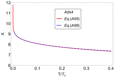
(a) $X$ vs $T/T_{c}$ at $\Delta=3/2$

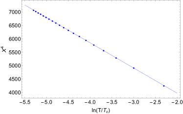
(b) $X^{4}$-$\log(T/T_{c})$ graph at $\Delta=3/2$.

Figure 15: (a) $X$ vs $T/T_{c}$: red colored curves for $X$ is a plot of Eq.(107). And blue dashed curves is a plot of Eq.(108). These two curves are almost indentical for low temperature.
(b)$X^{4}$-$\log(T/T_{c})$ graph at $\Delta=3/2$: The slope of blue dotted line for $X^{4}$ is $-939$.

A.1.3 Analytic calculation of $g^{\frac{1}{\Delta}}\frac{\left<\mathcal{O}_{\Delta}\right>^{\frac{1}{\Delta}}}{\sqrt{g\rho}}$ at $1/2<\Delta<3$

Apply Eq.(100) into Eq.(101) with $T=\frac{3}{4\pi}r_{h}$ with $b=\left(\frac{g\left<\mathcal{O}_{\Delta}\right>}{\Delta r_{h}^{\Delta}}\right)^{\frac{1}{\Delta}}$ in the form of $Y$; here, $Y:=$ $\frac{g^{1/\Delta}\left<\mathcal{O}_{\Delta}\right>^{1/\Delta}}{\sqrt{g\rho}}$ for simple notation, we obtain the condensate at $T\approx 0$:

$$Y^{4}=\widetilde{G_{3}}^{4}\left(\alpha_{3}+\beta_{3}\widetilde{\tau_{3}}^{3-2\Delta}Y^{3-2\Delta}\right)$$ (109)

$$\hbox{where }\quad\widetilde{G_{3}} = \Delta^{1/\Delta}\left(\frac{-2^{1+\nu}}{\Gamma(-\nu)}\right)^{\frac{1}{2}}$$ (110)

$$\widetilde{\tau_{3}} = \frac{d}{4\pi\Delta^{1/\Delta}}\frac{\sqrt{g\rho}}{T}$$ (111)

with $\nu=\frac{1}{2\Delta}$. Here, $\alpha_{3}$ and $\beta_{3}$ are in Eq.(103).

A.1.4 Analytic calculation of $g^{\frac{1}{\Delta}}\frac{\left<\mathcal{O}_{\Delta}\right>^{\frac{1}{\Delta}}}{\sqrt{g\rho}}$ at $\Delta=3/2$

As Eq.(104) and Eq.(105) are substituted into Eq.(109) with taking the limit $\Delta\rightarrow 3/2$, we obtain

$$Y^{4}=\widetilde{G_{3}}^{4}\left(\rho_{3}+\frac{\sigma_{3}}{2}\left(\frac{1-\widetilde{\tau_{3}}^{3-2\Delta}X^{3-2\Delta}}{\Delta-\frac{3}{2}}\right)\right).$$ (112)

By using L’Hopital’s rule, Eq.(112) becomes

$$Y^{4} = \widetilde{G_{3}}^{4}\left(\rho_{3}-\frac{\sigma_{3}}{2}\frac{\partial}{\partial\Delta}\left(\widetilde{\tau_{3}}^{3-2\Delta}Y^{3-2\Delta}\right)\right)$$ (113)

$$= \widetilde{G_{3}}^{4}\left(\rho_{3}+\sigma_{3}\ln\left(\widetilde{\tau_{3}}Y\right)\right)$$

Fig. 16 (b) tells us that $Y\sim\ln(\sqrt{g\rho}/T)^{1/4}$ for low temperature; Numerical result tells us that $Y^{4}$-$\log(T/\sqrt{g\rho})$ plot demonstrates our arguements with high precision.

And $Y$ is numerically

$$Y \approx 0.44\left(1+13.47\ln\left(\frac{\sqrt{g\rho}}{T}\right)\right)^{1/4}$$ (114)

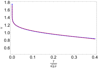
(a) $Y$ vs $T/\sqrt{g\rho}$ at $\Delta=3/2$

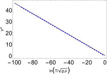
(b) $Y^{4}$-$\log(T/\sqrt{g\rho})$ graph at $\Delta=3/2$.

Figure 16: (a) $Y$ vs $T/\sqrt{g\rho}$: red colored curves for $Y$ is a plot of Eq.(113). And blue dashed curves is a plot of Eq.(114). These two curves are almost indentical for low temperature.
(b)$Y^{4}$-$\log(T/\sqrt{g\rho})$ graph at $\Delta=3/2$: The slope of blue dotted line for $Y^{4}$ is $-0.46$.

A.2 The Conductivity Gap

Now we begin to discuss the resonant frequencies. The Eq.(50) takes the form of a Schrödinger equation with energy $\omega$:

$$-\frac{d^{2}A_{x}}{dr_{\star}^{2}}+V(r_{\star})A_{x}=\omega^{2}A_{x},$$ (115)

where, $V(r_{\star})$ is re-expression of $V(z)=\frac{g^{2}\left<\mathcal{O}_{\Delta}\right>^{2}}{r_{+}^{2\Delta-2}}(1-z^{3})z^{2\Delta-2}F(z)^{2}$ in terms of the tortoise coordinate $r_{\star}$,

$$r_{\star}=\int\frac{dr}{f(r)}=\frac{1}{6r_{+}}\left[\ln\frac{(1-z)^{3}}{1-z^{3}}-2\sqrt{3}\tan^{-1}\frac{\sqrt{3}\;z}{2+z}\right],$$ (116)

where the integration constant is chosen such that boundary is at $r_{\star}=0$. We follow Horo2009 to define the size of the gap in AC conductivity $\omega_{g}$ by

$$\omega_{g}=\sqrt{V_{\mbox{max}}}.$$ (117)

Here, there is no solution for $\omega_{g}$ at $1/2<\Delta<1$. Because $\lim_{z\rightarrow 0}V(z)\rightarrow\infty$.jh Then, we can construct an analytic expression of $\omega_{g}$. First introduce $z_{0}$ at which $V$ is maximum:

$$\frac{dV}{dz}\Bigg{|}_{z=z_{0}}=\frac{d}{dz}(1-z^{3})z^{2\Delta-2}F(z)^{2}\Bigg{|}_{z=z_{0}}=0.$$ (118)

Then it can be numerically calculated as a function of $\Delta$ and $b$, and the result can be fit by following expressions.

$$z_{0} \approx 0.41\sum_{k=1}^{\infty}\frac{\sin\left(\pi(\Delta-1)(2k-1)\right)}{k^{2.64}},\;\;\hbox{ for }1\leq\Delta<2,$$ (119)

$$z_{0} \approx\left(\frac{0.10}{\Delta-1.83}+0.70\right)\frac{1}{b},\;\;\hbox{ for }2<\Delta\leq 3.$$ (120)

Notice that from the first expression, we can see that there is no $b$ dependence. This result is plotted in the Figure 17(a). Notice that the numerical data is fit very well by our formula.

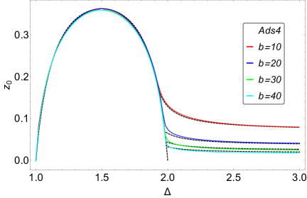
(a) $z_{0}$ vs $\Delta$.

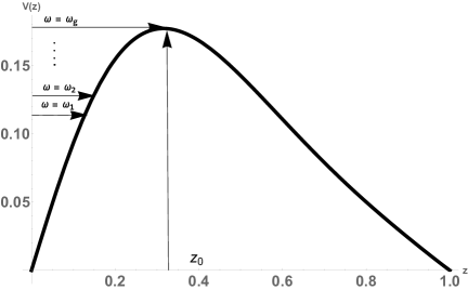
(b) $V(z)$ vs $z$.

Figure 17: (a) $z_{0}$ for various $b$’s. Solid colored curves are numerical expression Eq.(118) and dashed curves are analytic expression Eqs.(119, 120). The local maximum $z_{0}\approx 0.362$ is at $\Delta=3/2$. (b) a rough picture $V(z)$ in terms of a $z$ coordinate. $\omega=\omega_{g}$ at $z=z_{0}$. $\omega_{n}$ is the $n^{th}$ pole. $\omega_{1}<\omega_{2}<\cdots$ are resonant frequencies, but $\omega_{g}$ is the approximate value of the gap in AC conductivities.

Using these data, $\omega_{g}$ is given by

$$\omega_{g}=\sqrt{V_{\mbox{max}}}=\frac{g\left<\mathcal{O}_{\Delta}\right>}{r_{+}^{\Delta-1}}\sqrt{1-z_{0}^{3}}z_{0}^{\Delta-1}F(z_{0})\approx\frac{g\left<\mathcal{O}_{\Delta}\right>}{r_{+}^{\Delta-1}}z_{0}^{\Delta-1}F(z_{0}).$$ (121)

The expression for $F(z_{0})$ is cumbersome and it is given in the appendix A.3.1. The solution of Eq.(121) according to the regimes of $\Delta$ is given in Table. 3 ealier in the introduction and summary section. For derivation of these results, see the appendix A.3.1.

Using the result of the Cooper pair density $n_{s}$ given in Eq.(64) and the expression of $\omega_{g}$, we can calculate the ratio $n_{s}/\omega_{g}$. FIG. 18 is the plot of this result.

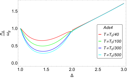
Figure 18: $n_{s}/\omega_{g}$ vs $\Delta$ for $d=3$. Here, $T_{0}=(g\rho)^{\frac{1}{2}}$. In the regime $2\leq\Delta\leq 3$, it is independent of $T$ but only $\Delta$ dependence.

Interestingly, in the regime $2\leq\Delta\leq 3$, we have linearity between ${n_{s}}$ and ${\omega_{g}}$.

$$\frac{n_{s}}{\omega_{g}}\approx 0.8\Delta-0.7,$$

Notice that in this regime of $\Delta$, there is no $b$ dependence in the ratio due to the cancellation of $b$-dependent pieces of $n_{s}$ and $\omega_{g}$.

A.2.1 Maxwell perturbations and the conductivity at near the zero temperature

The Maxwell equation at zero spatial momentum and with a time dependence of the form $e^{-i\omega t}$ gives

$$r_{+}^{2}(1-z^{3})^{2}\frac{d^{2}A_{x}}{dz^{2}}-3r_{+}^{2}z^{2}(1-z^{3})\frac{dA_{x}}{dz}+\left(\omega^{2}-V(z)\right)A_{x}=0$$

where $A_{x}$ is any component of the perturbing electromagnetic potential along the boundary and

$$V(z)=\frac{g^{2}\left<\mathcal{O}_{\Delta}\right>^{2}}{r_{+}^{2\Delta-2}}(1-z^{3})z^{2\Delta-2}F(z)^{2}$$

with $F$ defined before. We introduce $A_{x}(z)=(1-z^{3})^{-\frac{i}{3}\hat{\omega}}G(z)$ where $\hat{\omega}=\omega/r_{+}$. Because we require $A_{x}\propto(1-z^{3})^{-\frac{i}{3}\hat{\omega}}$ near $z=1$ corresponding to ingoing wave boundary conditions at the horizon. Then, the wave equation reads

$$(1-z^{3})\frac{d^{2}G}{dz^{2}}-3\left(1-\frac{2i\hat{\omega}}{3}\right)z^{2}\frac{dG}{dz}+\left(\frac{\hat{\omega}^{2}(1+z)(1+z^{2})}{1+z+z^{2}}+2i\hat{\omega}z-\frac{g^{2}\left<\mathcal{O}_{\Delta}\right>^{2}}{r_{+}^{2\Delta}}z^{2\Delta-2}F^{2}(z)\right)G=0$$

We have the following limiting form:

$$\lim_{z\rightarrow 0}K_{\nu}\left(z\right)\sim\frac{\Gamma(\nu)}{2}\left(\frac{z}{2}\right)^{-\nu}\sum_{k=0}^{1}\frac{\left(\frac{z}{2}\right)^{2k}}{(1-\nu)_{k}k!}+\frac{\Gamma(-\nu)}{2}\left(\frac{z}{2}\right)^{\nu}\sum_{k=0}^{1}\frac{\left(\frac{z}{2}\right)^{2k}}{(1+\nu)_{k}k!}$$ (122)

at $\nu\neq\mathbb{Z}$.

We obtain the analytic expressions of $F(z)$ in the following way:

$$F(z) \approx 1-\frac{(bz)^{4}\mathbb{J}_{1}+(bz)^{3}\mathbb{J}_{2}+(bz)^{2}\mathbb{J}_{3}}{-\frac{\sqrt{\pi}\Gamma\left(\frac{3}{2\Delta}-1\right)\Gamma\left(\frac{1}{\Delta}\right)\Gamma\left(\frac{2}{\Delta}\right)}{8\Delta^{2}\Gamma\left(\frac{\Delta+3}{2\Delta}\right)}+\frac{\pi(3-\Delta)^{2}\csc\left(\frac{\pi}{2\Delta}\right)}{4\Delta^{4}(3-2\Delta)}b^{3-2\Delta}},\;\;\hbox{ for }z\leq 1/b,$$ (123)

$$F(z) \approx 1-\frac{-\frac{\sqrt{\pi}\Gamma\left(\frac{3}{2\Delta}-1\right)\Gamma\left(\frac{1}{\Delta}\right)\Gamma\left(\frac{2}{\Delta}\right)}{8\Delta^{2}\Gamma\left(\frac{\Delta+3}{2\Delta}\right)}+\frac{\pi\csc\left(\frac{\pi}{2\Delta}\right)}{4\Delta^{2}(3-2\Delta)}(bz)^{3-2\Delta}}{-\frac{\sqrt{\pi}\Gamma\left(\frac{3}{2\Delta}-1\right)\Gamma\left(\frac{1}{\Delta}\right)\Gamma\left(\frac{2}{\Delta}\right)}{8\Delta^{2}\Gamma\left(\frac{\Delta+3}{2\Delta}\right)}+\frac{\pi(3-\Delta)^{2}\csc\left(\frac{\pi}{2\Delta}\right)}{4\Delta^{4}(3-2\Delta)}b^{3-2\Delta}},\;\;\hbox{ for }z>1/b.$$ (124)

where

$$\mathbb{J}_{1} = 2^{-\frac{1}{\Delta}-8}\Gamma\left(-1-\frac{1}{2\Delta}\right)^{2}\left(\frac{8\Delta+4}{\Delta^{2}}+\frac{8(2\Delta+1)(bz)^{2\Delta}}{\Delta\left(4\Delta^{2}+9\Delta+2\right)}+\frac{(bz)^{4\Delta}}{6\Delta^{2}+7\Delta+1}\right)$$

$$\mathbb{J}_{2} = -\frac{1}{24}\pi\csc\left(\frac{\pi}{2\Delta}\right)\left(\frac{\Delta^{2}\left(48\Delta+(2\Delta+3)(bz)^{2\Delta}+36\right)(bz)^{2\Delta}}{(2\Delta+3)(4\Delta+3)\left(4\Delta^{2}-1\right)}+4\right)$$

$$\mathbb{J}_{3} = 2^{\frac{1}{\Delta}-7}\Gamma\left(\frac{1}{2\Delta}-1\right)^{2}\left(\frac{8\Delta-4}{\Delta^{2}}+\frac{4(2\Delta-1)(bz)^{2\Delta}}{\Delta\left(4\Delta^{2}+3\Delta-1\right)}+\frac{(bz)^{4\Delta}}{12\Delta^{2}+4\Delta-1}\right)$$ (125)

As we apply Eq.(122) and Eq.(100) into Eq.(85a), we obtain Eq.(123).

Replacing $b$ by $bz$ in Eq.(87a) and Eq.(99), we have

$$F_{\Delta}(bz) = \int_{0}^{bz}dz\;z^{2-2\Delta}\int_{0}^{z}d\tilde{z}\;\tilde{z}^{2\Delta-1}\left(K_{\frac{1}{2\Delta}}\left(\tilde{z}^{\Delta}\right)\right)^{2}$$ (126)

$$= b^{3}\int_{0}^{z}dz\;z^{2-2\Delta}\int_{0}^{z}d\tilde{z}\;\tilde{z}^{2\Delta-1}\left(K_{\frac{1}{2\Delta}}\left(b^{\Delta}\tilde{z}^{\Delta}\right)\right)^{2}$$

$$= \frac{\pi\csc{\left(\frac{\pi}{2\Delta}\right)}}{4\Delta^{2}(3-2\Delta)}(bz)^{3-2\Delta}-\frac{\sqrt{\pi}\Gamma\left(\frac{3}{2\Delta}-1\right)\Gamma\left(\frac{1}{\Delta}\right)\Gamma\left(\frac{2}{\Delta}\right)}{8\Delta^{2}\Gamma\left(\frac{\Delta+3}{2\Delta}\right)}$$

Substitute Eq.(126) and Eq.(100) into Eq.(85a). We obtain Eq.(124).

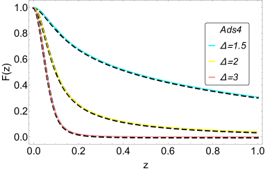
Figure 19: The field $F$ for $\Delta=1.5$ (light blue), $\Delta=2$ (yellow), $\Delta=3$ (pink) at $b=10$. Solid colored curves are analytic expression Eq.(123) and Eq.(124) and dashed curves are exact numerical results Eq.(85a) with Eq.(100) (almost indistinguishable).

Fig. 19 shows how the data fits by above formulas Eq.(123) and Eq.(124).

$F(z)\approx 1$ at $\Delta=1$ in Eq.(123) and Eq.(124). And the solution of Eq.(54) is

$$G(z)=\exp\left(iz\left(-\frac{\omega}{3}+\sqrt{\omega^{2}+\frac{i\omega}{3}-\frac{g^{2}\left<\mathcal{O}_{1}\right>^{2}}{r_{+}^{2}}}\right)\right)+R\;\exp\left(iz\left(-\frac{\omega}{3}-\sqrt{\omega^{2}+\frac{i\omega}{3}-\frac{g^{2}\left<\mathcal{O}_{1}\right>^{2}}{r_{+}^{2}}}\right)\right)$$ (127)

Here, $R$ is a reflection coefficient. $T\rightarrow 0$ is equivalent to sending the horizon to infinity. Then infalling boundary condition corresponds to $R=0$. Then it gives the conductivities to be

$$\sigma(\omega)=\frac{g\left<\mathcal{O}_{1}\right>}{\omega}\sqrt{\left(1+\frac{ir_{+}}{3\omega}\right)\left(\frac{\omega}{g\left<\mathcal{O}_{1}\right>}\right)^{2}-1}$$ (128)

via Eq.(53).

For $\Delta=2$ in Eq.(54), We may substitute the trial function

$$F(z)=\frac{\tanh(1.5bz)}{1.5bz}$$ (129)

which is satisfied with Eq.(123) and Eq.(124) numerically. Also, this trial function obey the correct boundary conditions ($F(0)=1$, $F^{\prime}(0)=1$ and $\lim_{z\rightarrow\infty}F(z)\propto(bz)^{3-2\Delta}$). Here, $b=\frac{\sqrt{g\left<\mathcal{O}_{2}\right>}}{\sqrt{2}r_{+}}$. Then at low temperature Eq.(54) reads

$$\frac{d^{2}G}{dz^{2}}+\frac{2i\hat{\omega}}{3}\frac{dG}{dz}+\left(\frac{8}{9}\hat{\omega}^{2}+\frac{i\hat{\omega}}{3}-\frac{16b^{2}}{9}\tanh^{2}(1.5bz)\right)G=0$$ (130)

whose general solution is given in terms of Legendre functions,

$$G(z)=\exp\left(-\frac{i\hat{\omega}z}{3}\right)P_{\nu}^{\mu}\left(\tanh(1.5bz)\right)+R\;\exp\left(-\frac{i\hat{\omega}z}{3}\right)P_{\nu}^{-\mu}\left(\tanh(1.5bz)\right)$$ (131)

where $\nu=\frac{-9+\sqrt{337}}{18}$ and $\mu=\frac{2i\sqrt{\hat{\omega}^{2}+\frac{i\hat{\omega}}{3}-\left(\frac{4}{3}b\right)^{2}}}{3b}$. Similar to $\Delta=1$, we choose infalling boundary condition corresponds to $R=0$. This exact result then produces the nonzero conductivities

$$\sigma(\omega) = \frac{3i\sqrt{g\left<\mathcal{O}_{2}\right>}}{\sqrt{2}\omega}\frac{\Gamma\left(\frac{1}{36}\left(27-\sqrt{337}-16i\sqrt{P(\omega)}\right)\right)\Gamma\left(\frac{1}{36}\left(27+\sqrt{337}-16i\sqrt{P(\omega)}\right)\right)}{\Gamma\left(\frac{1}{36}\left(9-\sqrt{337}-16i\sqrt{P(\omega)}\right)\right)\Gamma\left(\frac{1}{36}\left(9+\sqrt{337}-16i\sqrt{P(\omega)}\right)\right)}$$ (132)

$$= \frac{3i\sqrt{g\left<\mathcal{O}_{2}\right>}}{\sqrt{2}\omega}\frac{\Gamma\left(0.24-\frac{4i}{9}\sqrt{P(\omega)}\right)}{\Gamma\left(-0.26-\frac{4i}{9}\sqrt{P(\omega)}\right)}\frac{\Gamma\left(1.26-\frac{4i}{9}\sqrt{P(\omega)}\right)}{\Gamma\left(0.76-\frac{4i}{9}\sqrt{P(\omega)}\right)}$$

via Eq.(53) where

$$P(\omega)=\frac{9}{8}\left(1+\frac{ir_{+}}{3\omega}\right)\left(\frac{\omega}{\sqrt{g\left<\mathcal{O}_{2}\right>}}\right)^{2}-1.$$

Here we apply the following limiting form:

$$\lim_{z\rightarrow 0}P_{\nu}^{\mu}\left(z\right)=\frac{2^{\mu}\sqrt{2}}{\Gamma\left(1+\frac{\nu}{2}-\frac{\mu}{2}\right)\Gamma\left(\frac{1}{2}-\frac{\nu}{2}-\frac{\mu}{2}\right)}$$ (133)

The solution of Eq.(61) is

$$H_{0}(z)=\sqrt{bz}K_{\frac{1}{2\Delta}}\left(b^{\Delta}z^{\Delta}\right)+R\sqrt{bz}I_{\frac{1}{2\Delta}}\left(b^{\Delta}z^{\Delta}\right)$$ (134)

Here, we take $R=0$: The other solution $\sqrt{bz}I_{\frac{1}{2\Delta}}\left(b^{\Delta}z^{\Delta}\right)$ is rejected because it is is monotonically increasing as $z$ increases for large $b$. By substituting Eq.(134), the solution to the field equation Eq.(62) for $H_{1}$ is

$$H_{1}(z) = \sqrt{bz}K_{\frac{1}{2\Delta}}\left(b^{\Delta}z^{\Delta}\right)$$ (135)

$$+\frac{i\sqrt{b}}{6}z^{7/2}\left\{2\pi\csc\left(\frac{\pi}{2\Delta}\right)\left(I_{-\frac{1}{2\Delta}}\left(b^{\Delta}z^{\Delta}\right)+I_{\frac{1}{2\Delta}}\left(b^{\Delta}z^{\Delta}\right)\right){}_{2}F_{3}{\left[\genfrac{.}{.}{0.0pt}{}{\frac{1}{2}{\mathchar 44\relax}\mskip 4.0mu\frac{3}{2\Delta}}{1-\frac{1}{2\Delta}{\mathchar 44\relax}\mskip 4.0mu1+\frac{1}{2\Delta}{\mathchar 44\relax}\mskip 4.0mu1+\frac{3}{2\Delta}};b^{2\Delta}z^{2\Delta}\right]}\right.$$

$$-6\Delta\frac{2^{1/\Delta}}{\sqrt{bz}}\left(\Gamma\left(1+\frac{1}{2\Delta}\right)\right)^{2}I_{\frac{1}{2\Delta}}\left(b^{\Delta}z^{\Delta}\right){}_{2}F_{3}{\left[\genfrac{.}{.}{0.0pt}{}{\frac{1}{2}-\frac{1}{2\Delta}{\mathchar 44\relax}\mskip 4.0mu\frac{1}{\Delta}}{1-\frac{1}{\Delta}{\mathchar 44\relax}\mskip 4.0mu1-\frac{1}{2\Delta}{\mathchar 44\relax}\mskip 4.0mu1+\frac{1}{\Delta}};b^{2\Delta}z^{2\Delta}\right]}$$

$$\left.-3\Delta\frac{\sqrt{bz}}{2^{1/\Delta}}\left(\Gamma\left(1-\frac{1}{2\Delta}\right)\right)^{2}I_{-\frac{1}{2\Delta}}\left(b^{\Delta}z^{\Delta}\right){}_{2}F_{3}{\left[\genfrac{.}{.}{0.0pt}{}{\frac{1}{2}+\frac{1}{2\Delta}{\mathchar 44\relax}\mskip 4.0mu\frac{2}{\Delta}}{1+\frac{1}{\Delta}{\mathchar 44\relax}\mskip 4.0mu1+\frac{1}{2\Delta}{\mathchar 44\relax}\mskip 4.0mu1+\frac{2}{\Delta}};b^{2\Delta}z^{2\Delta}\right]}\right\}$$

Eq.(134) and Eq.(135) give us the nonzero conductivities

$$\lim_{\omega\rightarrow 0}\sigma(\omega)=\frac{2\pi\Delta\csc\left(\frac{\pi}{2\Delta}\right)}{(2\Delta)^{1/\Delta}\left(\Gamma\left(\frac{1}{2\Delta}\right)\right)^{2}}\frac{g^{1/\Delta}\left<\mathcal{O}_{\Delta}\right>^{1/\Delta}}{\omega}i$$ (136)

And we obtain

$$\frac{n_{s}}{T_{c}}=\frac{2\pi\Delta\csc\left(\frac{\pi}{2\Delta}\right)}{(2\Delta)^{1/\Delta}\left(\Gamma\left(\frac{1}{2\Delta}\right)\right)^{2}}\frac{g^{1/\Delta}\left<\mathcal{O}_{\Delta}\right>^{1/\Delta}}{T_{c}}$$ (137)

here, $n_{s}$ is also the coefficient of the pole in the imaginary part ${\rm Im}{\sigma(\omega)}\sim n_{s}/\omega$ as $\omega\rightarrow 0$.

A.3 The Resonant Frequencies

There is a maximum of $z_{0}$ at $\Delta=3/2$ and the resonance, by which $\sigma(\omega)$ diverges, occurs only in the vicinity of $\Delta=3/2$. This can be understood using standard WKB matching formula. The resonance occurs when there exists $\omega$ satisfying Horo2011

$$\int_{r_{*0}}^{0}\sqrt{\omega^{2}-V(r_{\star})}dr_{\star}+\frac{\pi}{4}=n\pi,$$

for an integer $n$ and $r_{*0}<0$ is the position at which $V$ has the maximum: $\frac{dV}{dr_{\star}}(r_{*0})=0$. The above equation can be converted to $z$ coordinate to give the following expression:

$$\frac{1}{r_{+}}\int_{0}^{z_{0}}\frac{\sqrt{\omega^{2}-V(z)}}{1-z^{3}}dz=\left(n-\frac{1}{4}\right)\pi.$$

At $\Delta=3/2$, we have

$$\int_{1/b}^{z_{0}}\sqrt{\left(\frac{\omega}{T_{c}}\right)^{2}-\left(\frac{2\pi}{3}\frac{T}{T_{c}}\right)^{2}b^{3}z\left(\frac{4-3\ln z}{2+\ln b}\right)^{2}}dz=\frac{4\pi^{2}}{3}\left(n-\frac{1}{4}\right)\frac{T}{T_{c}},$$ (138)

where $z_{0}=0.362$ from Eq.(119), and

$$b = 1.23\left(1+0.45\ln\left(\frac{T_{c}}{T}\right)\right)^{1/4}\frac{T_{c}}{T},$$

$$\frac{\omega_{g}}{T_{c}} = \frac{7}{10}\frac{{X^{3/2}\left(\frac{T_{c}}{T}\right)^{1/2}}}{\ln\left(X\frac{T_{c}}{T}\right)},\quad\hbox{ with }X=\frac{g^{1/\Delta}\left<\mathcal{O}_{\Delta}\right>^{1/\Delta}}{T_{c}}.$$

Resonant $\omega_{i}$’s exist only when $z_{0}$ is large enough. We can see that $z_{0}$ is maximum at $\Delta=3/2$ from the Fig 17(b). It turns out that only near the $\Delta=3/2$ because for other values which is much bigger or smaller than $z_{0}$, the barrier is too thick for the resonance to happen. For $\frac{T_{c}}{T}=0.1$, we have $\frac{\omega_{1}}{T_{c}}=10.44$ which is in good agreement with the ${\omega_{1}}/{T_{c}}=10.4$ Horo2009 if we set $g=1$. In general, as ${T}/{T_{c}}$ decreases, the number of poles increases. These results are summarized in the Table 4. For derivation of these results, see the appendix A.3.1.

Poles of $\sigma(\omega)$	$\frac{\omega_{1}}{T_{c}}$	$\frac{\omega_{2}}{T_{c}}$	$\frac{\omega_{3}}{T_{c}}$	$\frac{\omega_{4}}{T_{c}}$	$\frac{\omega_{5}}{T_{c}}$
$\frac{T}{T_{c}}=0.1$ with $\omega_{g}/T_{c}=10.9$	10.44
$\frac{T}{T_{c}}=0.05$ with $\omega_{g}/T_{c}=13.4$	11.85	13.11
$\frac{T}{T_{c}}=0.04$ with $\omega_{g}/T_{c}=14.62$	12.19	13.65	14.4
$\frac{T}{T_{c}}=0.03$ with $\omega_{g}/T_{c}=16.34$	12.6	14.26	15.21	15.84	16.25

Table 4: $\frac{\omega_{n}}{T_{c}}$ and $\frac{T}{T_{c}}$ at lower $T$’s. where $n=1,2,3,\cdots$. A position of the pole is obtained from Eq.(138) with given $\frac{T}{T_{c}}$ by applying Mathematica program.

A.3.1 Expression for the schrödinger wave equation of the conductivity at near the zero temperature

Eq.(50) takes the form of a schrödinger equation with energy $\omega$:

$$-\frac{d^{2}A_{x}}{dr_{\star}^{2}}+V(r_{\star})A_{x}=\omega^{2}A_{x}.$$

Here, $V(r_{\star})$ is re-expression of $V(z)=\frac{g^{2}\left<\mathcal{O}_{\Delta}\right>^{2}}{r_{+}^{2\Delta-2}}(1-z^{3})z^{2\Delta-2}F(z)^{2}$ in terms of the tortoise coordinate $r_{\star}$,

$$r_{\star}=\int\frac{dr}{f(r)}=\frac{1}{6r_{+}}\left[\ln\frac{(1-z)^{3}}{1-z^{3}}-2\sqrt{3}\tan^{-1}\frac{\sqrt{3}\;z}{2+z}\right],$$

where the integration constant is chosen such that boundary is at $r_{\star}=0$.

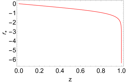
Figure 20: $r_{\star}$ vs $z$ Here, $r_{+}=1$ for simplicity.

FIG. 20. shows that the horizon corresponds to $r_{\star}=-\infty$. We can easily show that $V(r_{\star}=0)=0$ if $\Delta>1$, $V(r_{\star}=0)$ is a nonzero constant if $\Delta=1$, and $V(r_{\star})$ diverges as $r_{\star}\rightarrow 0$ if $1/2<\Delta<1$. FIG. 21. can show that $V(z)$ always vanishes at the horizon (or $V(r_{\star})$ vanishes at $r_{\star}\rightarrow-\infty$).

(a) $V(r_{\star})$ vs $r_{\star}$

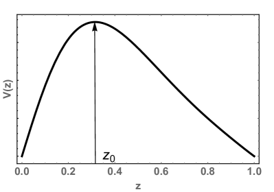
(b) $V(z)$ vs $z$.

Figure 21: (a) a rough picture $V(r_{\star})$ in terms of a $r_{\star}$ coordinate, (b) a rough picture $V(z)$ in terms of a $z$ coordinate.

The maximum value of $V(r_{\star})$ (or $V(z)$ ) always exists at $r_{\star}=r_{*0}$ (or $z=z_{0}$) if $\Delta\geq 1$. As we substitute Eq.(124) into Eq.(118), we obtain a polynomial equation such as

$$z_{0}^{2\Delta}(3-\Delta)^{2}(2+z_{0}^{3}+2\Delta(z_{0}^{3}-1))+\Delta^{2}z_{0}^{3}(4-2\Delta+(2\Delta-7)z_{0}^{3})=0.$$ (139)

And its numerical solution is

$$z_{0}\approx 0.41249\sum_{k=1}^{\infty}\frac{\sin\left(\pi(\Delta-1)(2k-1)\right)}{k^{2.6376}}$$ (140)

where $1\leq\Delta<2$. A dashed curve at $1\leq\Delta<2$ in FIG. 17 (a). indicates Eq.(140), and we see that there are no $b$ (or $T$) dependence.

As we substitute Eq.(123) into Eq.(118), we obtain a polynomial equation, and we see $z_{0}\propto 1/b$. Its numerical solution is

$$z_{0}\approx\left(\frac{0.1}{\Delta-1.83}+0.7\right)\frac{1}{b}$$ (141)

where $2\leq\Delta\leq 3$. A dashed curve at $2\leq\Delta\leq 3$ in FIG. 17. indicates Eq.(141), and we see that there are $b$ dependence.

And $\omega_{g}$ is given by

$$\omega_{g}=\sqrt{V_{\mbox{max}}}=\frac{g\left<\mathcal{O}_{\Delta}\right>}{r_{+}^{\Delta-1}}\sqrt{1-z_{0}^{3}}z_{0}^{\Delta-1}F(z_{0})\approx\frac{g\left<\mathcal{O}_{\Delta}\right>}{r_{+}^{\Delta-1}}z_{0}^{\Delta-1}F(z_{0}).$$ (142)

We obtain the analytic expressions of $\frac{\omega_{g}}{T_{c}}$ in the following way:

$$\frac{\omega_{g}}{T_{c}} =\left(\frac{3z_{0}}{4\pi}\frac{T_{c}}{T}\right)^{\Delta-1}\left(\frac{g^{1/\Delta}\left<\mathcal{O}_{\Delta}\right>^{1/\Delta}}{T_{c}}\right)^{\Delta}F_{<}(z_{0}),\;\;\hbox{ for }1\leq\Delta<2,$$ (143)

$$\frac{\omega_{g}}{T_{c}} =\left(\Delta^{1/\Delta}\rho_{\Delta}\right)^{\Delta-1}\frac{g^{1/\Delta}\left<\mathcal{O}_{\Delta}\right>^{1/\Delta}}{T_{c}}F_{>}(\rho_{\Delta}),\;\;\hbox{ for }2\leq\Delta\leq 3,$$ (144)

where

$$F_{<}(z_{0}) =1-\frac{-\frac{\sqrt{\pi}\Gamma\left(\frac{3}{2\Delta}-1\right)\Gamma\left(\frac{1}{\Delta}\right)\Gamma\left(\frac{2}{\Delta}\right)}{8\Delta^{2}\Gamma\left(\frac{\Delta+3}{2\Delta}\right)}+\frac{\pi\csc\left(\frac{\pi}{2\Delta}\right)}{4\Delta^{2}(3-2\Delta)}(bz_{0})^{3-2\Delta}}{-\frac{\sqrt{\pi}\Gamma\left(\frac{3}{2\Delta}-1\right)\Gamma\left(\frac{1}{\Delta}\right)\Gamma\left(\frac{2}{\Delta}\right)}{8\Delta^{2}\Gamma\left(\frac{\Delta+3}{2\Delta}\right)}+\frac{\pi(3-\Delta)^{2}\csc\left(\frac{\pi}{2\Delta}\right)}{4\Delta^{4}(3-2\Delta)}b^{3-2\Delta}},$$ (145)

$$F_{>}(\rho_{\Delta}) =1+\frac{\Delta^{2}\rho_{\Delta}^{2}\Gamma\left(\frac{3+\Delta}{2\Delta}\right)\left[\rho_{\Delta}\mathbb{M}_{1}+\rho_{\Delta}^{2}\mathbb{M}_{2}+\mathbb{M}_{3}\right]}{6\sqrt{\pi}\Gamma\left(\frac{1}{\Delta}\right)\Gamma\left(\frac{2}{\Delta}\right)\Gamma\left(-1+\frac{3}{2\Delta}\right)},$$ (146)

with

$$\mathbb{M}_{1} = 8\pi\csc\left(\frac{\pi}{2\Delta}\right)\left(-1+\frac{3\Delta^{2}\rho_{\Delta}^{2\Delta}}{3-2\Delta(4\Delta^{2}+6\Delta-1)}\right),$$

$$\mathbb{M}_{2} = \frac{3\left(\Gamma\left(\frac{-1}{2\Delta}\right)\right)^{2}}{2^{1/\Delta}}\left(\frac{2+\Delta(9+4\Delta+2\rho_{\Delta}^{2\Delta})}{(2+\Delta)(1+2\Delta)(1+4\Delta)}\right),$$

$$\mathbb{M}_{3} = 6\left(\Gamma\left(\frac{1}{2\Delta}\right)\right)^{2}2^{1/\Delta}\left(\frac{4\Delta^{2}-1+\Delta(3+\rho_{\Delta}^{2\Delta})}{8\Delta^{3}+2\Delta^{2}-5\Delta+1}\right),$$

$$\rho_{\Delta} = \left(\frac{0.1}{\Delta-1.83}+0.7\right).$$ (147)

Substitute Eq.(124) with Eq.(140) into Eq.(142) and we obtain Eq.(143). Also, substitute Eq.(123) with Eq.(141) into Eq.(142) and we obtain Eq.(144). A numerical result tells us that Eq.(144) approximately is

$$\frac{\omega_{g}}{T_{c}}\approx\frac{1.1}{\mbox{li}(\Delta^{1.2})}\frac{g^{1/\Delta}\left<\mathcal{O}_{\Delta}\right>^{1/\Delta}}{T_{c}},$$ (148)

here, $\mbox{li}(x)$ is an logarithmic integral function. See Fig.22.

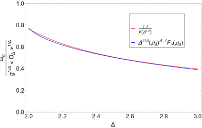
Figure 22: Solid red curve is a plot of $\frac{1.1}{\mbox{li}(\Delta^{1.2})}$ and blue one is a plot of $\left(\Delta^{1/\Delta}\rho_{\Delta}\right)^{\Delta-1}F_{>}(\rho_{\Delta})$ with Eq.(146) in Eq.(144) (almost indistinguishable).

And we can classify Eq.(143) into the following way:

1. As $1\leq\Delta\ll 3/2$,

   $$\frac{\omega_{g}}{T_{c}}=\left(\frac{3z_{0}}{4\pi}\frac{T_{c}}{T}\right)^{\Delta-1}\left(1-\left(\frac{\Delta}{3-\Delta}z_{0}^{3/2-\Delta}\right)^{2}\right)X^{\Delta}$$ (149)

2. As $\Delta=3/2$,

   $$\frac{\omega_{g}}{T_{c}}=\frac{7}{10}\frac{{X^{3/2}\left(\frac{T_{c}}{T}\right)^{1/2}}}{\ln\left(X\frac{T_{c}}{T}\right)}$$ (150)

3. As $3/2\ll\Delta<2$,

   $$\frac{\omega_{g}}{T_{c}}=\left(\frac{3z_{0}}{4\pi}\frac{T_{c}}{T}\right)^{2-\Delta}\frac{\sqrt{\pi}\Gamma\left(\frac{3+\Delta}{2+\Delta}\right)\csc\left(\frac{\pi}{2\Delta}\right)}{\Delta^{3/\Delta}\Gamma\left(\frac{2}{\Delta}\right)\Gamma\left(\frac{3}{2\Delta}\right)\Gamma\left(1+\frac{1}{\Delta}\right)}\left(1-\left(\frac{\Delta}{3-\Delta}z_{0}^{\Delta-3/2}\right)^{2}\right)X^{3-\Delta}$$ (151)

Here, $X=\frac{g^{1/\Delta}\left<\mathcal{O}_{\Delta}\right>^{1/\Delta}}{T_{c}}$.

From Eq.(137), Eq.(149), Eq.(150) and Eq.(151) , we find a relation between $n_{s}$ and the gap frequency $\omega_{g}$:

1. As $1\leq\Delta\ll 3/2$,

   $$\frac{n_{s}}{\omega_{g}}=\frac{2\pi\Delta\csc\left(\frac{\pi}{2\Delta}\right)}{(2\Delta)^{1/\Delta}\left(\Gamma\left(\frac{1}{2\Delta}\right)\right)^{2}}\frac{1}{1-\left(\frac{\Delta}{3-\Delta}z_{0}^{3/2-\Delta}\right)^{2}}\left(\frac{3z_{0}}{4\pi}X\right)^{1-\Delta}$$ (152)

2. As $\Delta=3/2$,

   $$\frac{n_{s}}{\omega_{g}}=\frac{\ln\left(X\frac{T_{c}}{T}\right)}{\sqrt{X\frac{T_{c}}{T}}}$$ (153)

3. As $3/2\ll\Delta<2$,

   $$\frac{n_{s}}{\omega_{g}}=\frac{2\sqrt{\pi}\Delta^{1+3/\Delta}}{(2\Delta)^{1/\Delta}\left(\Gamma\left(\frac{1}{2\Delta}\right)\right)^{2}}\frac{\Gamma\left(\frac{2}{\Delta}\right)\Gamma\left(\frac{3}{2\Delta}\right)\Gamma\left(1+\frac{1}{\Delta}\right)}{\Gamma\left(\frac{3+\Delta}{2\Delta}\right)}\frac{1}{1-\left(\frac{\Delta}{3-\Delta}z_{0}^{\Delta-3/2}\right)^{2}}\left(\frac{3z_{0}}{4\pi}X\right)^{\Delta-2}$$ (154)

4. As $2\leq\Delta\leq 3$,

   $$\frac{n_{s}}{\omega_{g}}=\frac{2\pi\Delta\csc\left(\frac{\pi}{2\Delta}\right)}{1.1(2\Delta)^{1/\Delta}\left(\Gamma\left(\frac{1}{2\Delta}\right)\right)^{2}}\mbox{li}(\Delta^{1.2})$$ (155)

A numerical result tells us that Eq.(155) is approximately

$$\frac{n_{s}}{\omega_{g}}\approx 0.8\Delta-0.7,$$ (156)

here, $z_{0}$ is Eq.(140). See Fig.23.

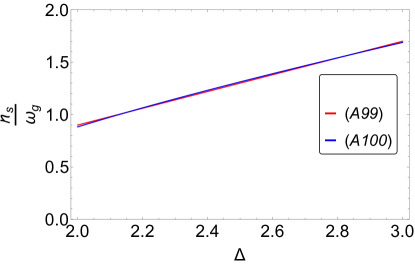
Figure 23: Solid red curve is a plot of Eq.(155) and blue one is a plot of Eq.(156) (almost indistinguishable).

As we see Fig 2. Horo2009 , $\sigma(\omega)$ has a spike at $\frac{\omega}{T_{c}}\approx 10.4$ and $\Delta=3/2$ for $AdS_{4}$. In FIG. 21 (b), resonance occurs well when the distance between $z=0$ and $z=z_{0}$ is the maximum. FIG. 17 (a) shows that there is a maximum of $z_{0}$ at $\Delta=3/2$. So, the resonance, by which $\sigma(\omega)$ diverges, occurs only in the vicinity of $\Delta=3/2$. This can be understood using standard WKB matching formula: The resonance occurs when there exists $\omega$ satisfying Horo2011

$$\int_{r_{*0}}^{0}\sqrt{\omega^{2}-V(r_{\star})}dr_{\star}+\frac{\pi}{4}=n\pi,$$ (157)

for an integer $n$ and $r_{*0}<0$ is the position at which $V$ has the maximum: $\frac{dV}{dr_{\star}}(r_{*0})=0$. The above equation can be converted to $z$ coordinate to give the following expression:

$$\frac{1}{r_{+}}\int_{0}^{z_{0}}\frac{\sqrt{\omega^{2}-V(z)}}{1-z^{3}}dz=\left(n-\frac{1}{4}\right)\pi.$$ (158)

By applying Eq.(124) into Eq.(158), we obtain

$$\frac{1}{r_{+}}\int_{0}^{z_{0}}\frac{\sqrt{\omega^{2}-V(z)}}{1-z^{3}}dz\approx\frac{1}{r_{+}}\int_{1/b}^{z_{0}}\frac{\sqrt{\omega^{2}-\left(\frac{g\left<\mathcal{O}_{\Delta}\right>}{r_{+}^{\Delta-1}}\right)^{2}z^{2\Delta-2}(1-z^{3})\left(\frac{(\beta-\beta_{0}z^{3-2\Delta})b^{3-2\Delta}}{\alpha+\beta b^{3-2\Delta}}\right)^{2}}}{1-z^{3}}dz$$ (159)

$$\approx \frac{1}{r_{+}}\int_{1/b}^{z_{0}}\sqrt{\omega^{2}-\left(\frac{g\left<\mathcal{O}_{\Delta}\right>}{r_{+}^{\Delta-1}}\right)^{2}z^{2\Delta-2}\left(\frac{(\beta-\beta_{0}z^{3-2\Delta})b^{3-2\Delta}}{\alpha+\beta b^{3-2\Delta}}\right)^{2}}dz=\left(n-\frac{1}{4}\right)\pi,$$

where

$$\alpha = -\frac{\sqrt{\pi}\Gamma\left(\frac{3}{2\Delta}-1\right)\Gamma\left(\frac{1}{\Delta}\right)\Gamma\left(\frac{2}{\Delta}\right)}{8\Delta^{2}\Gamma\left(\frac{\Delta+3}{2\Delta}\right)},$$

$$\beta = \frac{\pi(3-\Delta)^{2}\csc\left(\frac{\pi}{2\Delta}\right)}{4\Delta^{4}(3-2\Delta)},$$

$$\beta_{0} = \frac{\pi\csc\left(\frac{\pi}{2\Delta}\right)}{4\Delta^{2}(3-2\Delta)}.$$ (160)

At $\Delta=3/2$, Eq.(159) becomes

$$\int_{1/b}^{z_{0}}\sqrt{\left(\frac{\omega}{T_{c}}\right)^{2}-\left(\frac{2\pi}{3}\frac{T}{T_{c}}\right)^{2}b^{3}z\left(\frac{4-3\ln z}{2+\ln b}\right)^{2}}dz=\frac{4\pi^{2}}{3}\left(n-\frac{1}{4}\right)\frac{T}{T_{c}},$$ (161)

where $z_{0}=0.362$ from Eq.(119), and

$$b = 1.23\left(1+0.45\ln\left(\frac{T_{c}}{T}\right)\right)^{1/4}\frac{T_{c}}{T},$$

$$\frac{\omega_{g}}{T_{c}} = \frac{7}{10}\frac{{X^{3/2}\left(\frac{T_{c}}{T}\right)^{1/2}}}{\ln\left(X\frac{T_{c}}{T}\right)},\quad\hbox{ with }X=\frac{g^{1/\Delta}\left<\mathcal{O}_{\Delta}\right>^{1/\Delta}}{T_{c}}.$$ (162)

Here, Eq.(162) is derived from Eq.(108).

Poles of $\sigma(\omega)$	$\frac{\omega_{1}}{T_{c}}$	$\frac{\omega_{2}}{T_{c}}$	$\frac{\omega_{3}}{T_{c}}$	$\frac{\omega_{4}}{T_{c}}$	$\frac{\omega_{5}}{T_{c}}$	$\frac{\omega_{6}}{T_{c}}$	$\frac{\omega_{7}}{T_{c}}$	$\frac{\omega_{8}}{T_{c}}$	$\frac{\omega_{9}}{T_{c}}$
$\frac{T}{T_{c}}=0.1$ with $\omega_{g}/T_{c}=10.9$	10.44
$\frac{T}{T_{c}}=0.05$ with $\omega_{g}/T_{c}=13.4$	11.85	13.11
$\frac{T}{T_{c}}=0.04$ with $\omega_{g}/T_{c}=14.62$	12.19	13.65	14.4
$\frac{T}{T_{c}}=0.03$ with $\omega_{g}/T_{c}=16.34$	12.6	14.26	15.21	15.84	16.25
$\frac{T}{T_{c}}=0.02$ with $\omega_{g}/T_{c}=19.18$	13.11	15.0	16.15	16.97	17.6	18.1	18.5	18.82	19.07

Table 5: $\frac{\omega_{n}}{T_{c}}$ and $\frac{T}{T_{c}}$ at lower $T$’s. where $n=1,2,3,\cdots$. A position of the pole is obtained from Eq.(161) with given $\frac{T}{T_{c}}$ by applying Mathematica program.

Appendix B Holographic superconductors with AdS₅

B.1 Near the critical temperature

B.1.1 Computation of $T_{c}$ by applying matrix algorithm and Pincherle’s Theorem

At the critical temperature $T_{c}$, $\Psi=0$, so Eq.(3) tells us $\Phi^{{}^{\prime\prime}}=0$. Then, we can set

$$\Phi(z)=\lambda_{4}r_{c}(1-x)\hskip 28.45274pt\mbox{where}\;\;\lambda_{4}=\frac{\rho}{r_{c}^{3}}$$ (163)

where $x=z^{2}$. As $T\rightarrow T_{c}$, the field equation $\Psi$ approaches to

$$-\frac{d^{2}\Psi}{dx^{2}}+\frac{1+x^{2}}{x(1-x^{2})}\frac{d\Psi}{dx}+\frac{m^{2}}{4x^{2}(1-x^{2})}\Psi=\frac{\lambda_{g,4}^{2}}{4x(1+x)^{2}}\Psi$$ (164)

where $\lambda_{g,4}=g\lambda_{4}$. Factoring out the behavior near the boundary $z=0$ and the horizon, we define

$$\Psi(x)=\frac{\left<\mathcal{O}_{\Delta}\right>}{\sqrt{2}r_{h}^{\Delta}}x^{\frac{\Delta}{2}}F(x)\hskip 28.45274pt\mbox{where}\;\;F(x)=(1+x)^{-\lambda_{g,4}/2}y(x)$$ (165)

Then, $F$ is normalized as $F(0)=1$ and we obtain

$$\frac{d^{2}y}{dx^{2}}+\left(\frac{\Delta-1}{x}+\frac{1}{x-1}+\frac{1-\lambda_{g,4}}{x+1}\right)\frac{dy}{dx}+\frac{\frac{(\Delta-\lambda_{g,4})^{2}}{4}x-\frac{\lambda_{g,4}}{2}\left(\frac{\lambda_{g,4}}{2}-\Delta+1\right)}{x(x-1)(x+1)}y=0.$$ (166)

Eq.(166) is the Heun differential equation that has four regular singular points at $z=0,1,-1,\infty$ Ronv1995 . Substituting $y(x)=\sum_{n=0}^{\infty}d_{n}x^{n}$ into (166), we obtain the following three term recurrence relation:

$$\alpha_{n}\;d_{n+1}+\beta_{n}\;d_{n}+\gamma_{n}\;d_{n-1}=0\quad\hbox{ for }n\geq 1,$$ (167)

with

$$\begin{cases}\alpha_{n}=(n+1)(n+\Delta-1)\cr\beta_{n}=-\frac{\lambda_{g,4}}{2}\left(2n+\Delta-1-\frac{\lambda_{g,4}}{2}\right)\cr\gamma_{n}=-\left(n-1+\frac{\Delta}{2}-\frac{\lambda_{g,4}}{2}\right)^{2}\end{cases}$$ (168)

The first three $d_{n}$’s are given by $\alpha_{0}d_{1}+\beta_{0}d_{0}=0$ and $d_{-1}=0$. Eq.(165), Eq.(167) and Eq.(168) tells us the following boundary condition

$$F^{{}^{\prime}}(0)=0.$$ (169)

We rewrite Eq.(167) as

$$d_{n+1}+A_{n}\;d_{n}+B_{n}\;d_{n-1}=0,$$ (170)

where $A_{n}$ and $B_{n}$ have asymptotic expansions of the form

$$\begin{cases}A_{n}=\frac{\beta_{n}}{\alpha_{n}}\sim\sum_{j=0}^{\infty}\frac{a_{j}}{n^{j}}\cr B_{n}=\frac{\gamma_{n}}{\alpha_{n}}\sim\sum_{j=0}^{\infty}\frac{b_{j}}{n^{j}}\end{cases}$$ (171)

with

$$\begin{cases}a_{0}=0,\quad a_{1}=-\lambda_{g,4},\quad a_{2}=\frac{\lambda_{g,4}}{2}\left(\Delta+1+\frac{\lambda_{g,4}}{2}\right)\cr b_{0}=-1,\quad b_{1}=2+\lambda_{g,4},\quad b_{2}=\frac{1}{4}\left(\lambda_{g,4}+\Delta\right)^{2}+2+\lambda_{g,4}\end{cases}$$ (172)

The radius of convergence, $\rho$, satisfies characteristic equation associated with Eq.(170) Miln1933 ; Perr1921 ; Poin1885 :

$$\rho^{2}+a_{0}\rho+b_{0}=\rho^{2}-1=0,$$ (173)

whose roots are given by

$$\rho_{1}=1\hskip 28.45274pt\rho_{2}=-1$$ (174)

So for a three–term recurrence relation in Eq.(167), the radius of convergence is 1 for all two cases. Since the solutions should converge at the horizon, $y(z)$ should be convergent at $|z|\leq 1$. According to Pincherle’s Theorem Jone1980 , we have a convergent solution of $y(z)$ at $|z|=1$ if only if the three term recurrence relation Eq.(167) has a minimal solution. Since we have two different roots $\rho_{i}$’s, so Eq.(170) has two linearly independent solutions $d_{1}(n)$, $d_{2}(n)$. One can show that Jone1980 for large $n$,

$$d_{i}(n)\sim\rho_{i}^{n}n^{\alpha_{i}}\sum_{r=0}^{\infty}\frac{\tau_{i}(r)}{n^{r}},\quad i=1,2,3$$ (175)

with

$$\alpha_{i}=\frac{a_{1}\rho_{i}+b_{1}}{a_{0}\rho_{i}+2b_{0}},\quad i=1,2$$ (176)

and $\tau_{i}(0)=1$. In particular, we obtain

$$\tau_{i}(1)=\frac{-2\rho_{i}^{2}\alpha_{i}(\alpha_{i}-1)-\rho_{i}(a_{2}+\rho_{i}a_{1}+\alpha_{i}(\alpha_{i}-1)a_{0}/2)-b_{2}}{2\rho_{i}^{2}(\alpha_{i}-1)+\rho_{i}(a_{1}+(\rho_{i}-1)a_{0})+b_{1}},\quad i=1,2$$ (177)

Substituting Eq.(174) and Eq.(172) into Eq.(175)–Eq.(177), we obtain

$$\begin{cases}d_{1}(n)\sim n^{-1}\left(1+\frac{\Delta^{2}+4\Delta\lambda_{g,4}+2(\lambda_{g,4}^{2}+\lambda_{g,4}+12)}{8n}\right)\cr d_{2}(n)\sim(-1)^{n}n^{-1-\lambda_{g,4}}\left(1+\frac{\lambda_{g,4}^{2}+\frac{11}{4}\lambda_{g,4}+\frac{\Delta^{2}}{8}+3}{n}\right)\end{cases}$$ (178)

Since $\lambda_{g,4}>0$,

$$\lim_{n\rightarrow\infty}\frac{d_{2}(n)}{d_{1}(n)}=0.$$ (179)

So $d_{2}(n)$ is a minimal solution. Also,

$$\begin{cases}\sum|d_{1}(n)|\sim\sum\frac{1}{n}\rightarrow\infty\cr\sum|d_{2}(n)|\sim\sum n^{-1-\lambda_{g,4}}<\infty\end{cases}$$ (180)

Therefore, $y(z)=\sum_{n=0}^{\infty}d_{n}x^{n}$ is convergent at $x=1$ if only if $d_{n}$ is a minimal solution. Eq.(21) with $\delta_{2}=\delta_{3}=\cdots=\delta_{N}=0$ becomes a polynomial of degree $N$ with respect to $\lambda_{g,4}$. Put Eq.(168) into Eq.(21) where $\delta_{i}=0$ at $i\in\{2,3,\cdots,N\}$ and we choose $N=15$

For algorithm to find $\lambda_{g,4}$ for a given $\Delta$,

1. Choose an $N$.

2. Put Eq.(168) into Eq.(21).

3. Define a function returning the determinant of system Eq.(21).

4. Find the roots of interest of this function.

5. Increase $N$ until those roots become constant to within the desired precision Leav1990 .

B.1.2 Unphysical region of $\Delta$

We use Mathematica to compute the determinants to locate their roots. We are only interested in smallest positive real roots of $\lambda_{g,4}$. For computation of roots, we choose $N=30$. For the smallest value of $\lambda_{g,4}$, we can find an approximate fitting function that is given by

$$\lambda_{g,4}\approx 1.18\Delta^{4/3}-0.97\;\;\mbox{at}\;\;3/2\leq\Delta\leq 4$$ (181)

Fig. 24 shows us that there is no convergent solution for $1<\Delta<3/2$. Because there are two branches, and these branches does not converge to single value $\lambda_{g,4}$ no matter how we increase $N$.

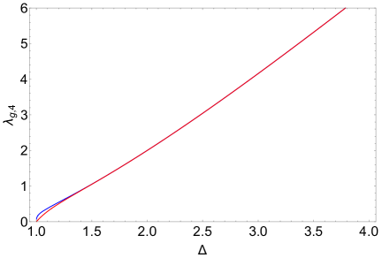
(a) $\lambda_{g,4}$ vs $\Delta$.

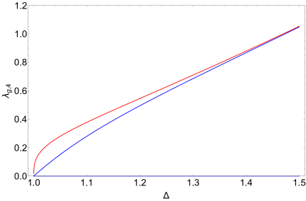
(b) $\lambda_{g,4}$ vs $\Delta$.

Figure 24: (a) $\lambda_{g,4}$ vs $\Delta$: Blue and red colored curves for $\lambda_{g,4}$ are obtained by letting $d_{N}=0$, with $N=29,30$ respectively. There are two branches in $1<\Delta<3/2$. And such brances merge for $\Delta\geq 3/2$. (b) Zoom in on the left plot.

Fig. 24 shows that these two branches merge to the single value $\lambda_{g,4}\approx 1$ as $N$ increases. We are interested why two branches occur near $\Delta=1$ regardless of the size of $N$.

Eq.(21) can be simplified using the formula for the determinant of a block matirix,

$$\det\begin{pmatrix}A&B\\ C&D\end{pmatrix}=\det(A)\det(D-CA^{-1}B),\quad{\rm with}$$ (182)

$\footnotesize A=\begin{pmatrix}\beta_{0}&\alpha_{0}\\ \gamma_{1}&\beta_{1}\end{pmatrix},\quad B=\begin{pmatrix}0&0&\cdots&0\\ \alpha_{1}&0&\cdots&0\end{pmatrix},\quad C=\begin{pmatrix}0&\gamma_{2}\\ 0&0\\ 0&0\\ 0&0\\ \vdots&\vdots\\ 0&0\end{pmatrix},\quad D=\begin{pmatrix}\beta_{2}&\alpha_{2}&&&&\\ \gamma_{3}&\beta_{3}&\alpha_{3}&&&\\ &\gamma_{4}&\beta_{4}&\alpha_{4}&&\\ &&\ddots&\ddots&\ddots&\\ &&&\gamma_{N-1}&\beta_{N-1}&\alpha_{N-1}\\ &&&&\gamma_{N}&\beta_{N}\end{pmatrix}.$ By explicit computation, we can see the factor $\det(A)=\frac{\lambda^{3}}{16}(\lambda-4)$ at $\Delta=1$ so that the minimal real root is $\lambda_{g,4}=0$. Near $\Delta=1$, we can expand the determinant as a series in $\varepsilon=\Delta-1\ll 1$ and $0<\lambda_{g,4}\ll 1$. After some calculations, we found that $d_{N}=0$ gives following results:

1. For $N=2m$ where $m=1,2,3,\cdots$,

   $$\lambda_{g,4}^{2}\sum_{n=0}^{2N}\alpha_{0,n}\lambda_{g,4}^{n}+\varepsilon\lambda_{g,4}\sum_{n=0}^{2N}\beta_{0,n}\lambda_{g,4}^{n}+\mathcal{O}(\varepsilon^{2})=0$$

   This leads us $\lambda_{g,4}\sim\varepsilon\sim(\Delta-1)$ as far as $\alpha_{0,0}\beta_{0,0}\neq 0$, which can be confirmed by explicit computation.

2. For $N=2m+1$,

   $$\lambda_{g,4}^{3}\sum_{n=0}^{2N-1}\alpha_{1,n}\lambda_{g,4}^{n}+\varepsilon\sum_{n=0}^{2N+1}\beta_{1,n}\lambda_{g,4}^{n}+\mathcal{O}(\varepsilon^{2})=0$$

   leading to $\lambda_{g,4}\sim(\Delta-1)^{1/3}$.

This proof tells us that two branches should be occured near $\Delta=1$.

We calculated 121 different values of $\lambda_{g,4}$’s at various $\Delta$ and the result is the blue colored curves in Fig. 3. These data fits well by above formula.

The authors of refSiop2012 got $\lambda_{g,4}$’s by using variational method using the fact that the eigenvalue $\lambda_{g,4}$ minimizes the expression

$$\lambda_{g,4}^{2}=\frac{\int_{0}^{1}dz\;z^{2\Delta-3}\left((1-z^{4})\left[F^{{}^{\prime}}(z)\right]^{2}+\Delta^{2}z^{2}\left[F(z)\right]^{2}\right)}{\int_{0}^{1}dz\;z^{2\Delta-3}\frac{1-z^{2}}{1+z^{2}}\left[F(z)\right]^{2}}$$ (183)

for $\Delta>1$. This integral does not converge at $\Delta=1$ because of $\ln(z)$. The trial function used is $F(z)=1-\alpha z^{3}$ where $\alpha$ is the variational parameter. Their result is given by the green colored dots in Fig. 3 and ours by the blue curves. The differences are appreciable at $\Delta>1.8$. Our results are consistently lower. The variational method show us that there are numerical values of $\lambda_{g,4}$ for $1<\Delta<3/2$. But our method tells us that the region $1<\Delta<3/2$ is not valid for analytic solutions because of non-convergence $\lambda_{g,4}$.

The critical temperature which is given by $T_{c}=\frac{1}{\pi}r_{c}=\frac{1}{\pi}\left(\frac{\rho}{\lambda_{4}}\right)^{\frac{1}{3}}$ which can be calculated by Eq.(181) and the Fig. 3(b) demonstrate the result. Notice that figure 1 in ref. siopsis2011holographic show us that $T_{c}$ is divergent at $\Delta=1$ and it is a monotonically decreasing function of $\Delta$.

B.1.3 The analytic solution of $g\frac{\left<\mathcal{O}_{\Delta}\right>}{T_{c}^{\Delta}}$

Substituting Eq.(165) into Eq.(3), the field equation $\Phi$ becomes

$$\frac{d^{2}\Phi}{dx^{2}}=\frac{g^{2}\left<\mathcal{O}_{\Delta}\right>^{2}}{4r_{h}^{2\Delta}}\frac{x^{\Delta-2}F^{2}(x)}{1-x^{2}}\Phi$$ (184)

where $\frac{g^{2}\left<\mathcal{O}_{\Delta}\right>^{2}}{4r_{h}^{2\Delta}}$ is small because of $T\approx T_{c}$. The above equation has the expansion around Eq.(163) with small correction:

$$\frac{\Phi}{r_{h}}=\lambda_{4}(1-x)+\frac{g^{2}\left<\mathcal{O}_{\Delta}\right>^{2}}{4r_{h}^{2\Delta}}\chi_{1}(z)$$ (185)

We have $\chi_{1}(1)=\chi_{1}^{{}^{\prime}}(1)=0$ due to the boundary conditions $\Phi(1)=0$ . Taking derivative of Eq.(185) twice with respect to $x$ and using the result in Eq.(184),

$$\chi_{1}^{{}^{\prime\prime}}=\frac{x^{\Delta-2}F^{2}(z)}{1-x^{2}}\left\{\lambda_{4}(1-x)+\frac{g^{2}\left<\mathcal{O}_{\Delta}\right>^{2}}{4r_{h}^{2\Delta}}\chi_{1}\right\}\approx\frac{\lambda_{4}x^{\Delta-2}F^{2}(z)}{1+x}.$$ (186)

Integrating Eq.(186) gives us

$$\chi_{1}^{{}^{\prime}}(0)=-\lambda_{4}\mathcal{C}_{4}\quad\hbox{ for }\mathcal{C}_{4}=\int_{0}^{1}dx\;\frac{x^{\Delta-2}F^{2}(x)}{1+x}$$ (187)

Eq.(165) with Eq.(168) shows

$$F(z)=(1+x)^{-\lambda_{g,4}/2}y(x)\approx(1+x)^{-\lambda_{g,4}/2}\sum_{n=0}^{10}d_{n}x^{n}$$ (188)

Here, we ignore $d_{n}x^{n}$ terms if $n\geq 11$ because $0<|d_{n}|\ll 1$ numerically and $y(x)$ converges at $0\leq x\leq 1$. We can calculate the numerical value of $\mathcal{C}_{4}$ by putting Eq.(181) and Eq.(168) into Eq.(187). We calculated 121 different values of $\sqrt{1/\mathcal{C}_{4}}$’s at various $\Delta$, which is drawn as dots in Fig. 4. Then we tried to find an approximate fitting function. The result is given as follows,

$$\sqrt{\frac{1}{\mathcal{C}_{4}}}\approx\frac{\Delta^{6.5}+510\Delta^{2}}{1327}$$ (189)

The Fig. 4 shows how the data fits by above formula. From Eq.(185) and Eq.(4), we have

$$\frac{\rho}{r_{h}^{3}}=\lambda_{4}\left(1+\frac{\mathcal{C}_{4}g^{2}\left<\mathcal{O}_{\Delta}\right>^{2}}{4r_{h}^{2\Delta}}\right)$$ (190)

Putting $T=\frac{1}{\pi}r_{h}$ with $\lambda_{4}=\frac{\rho}{r_{c}^{3}}$ into Eq.(190), we obtain the condensate near $T_{c}$:

$$g\frac{\left<\mathcal{O}_{\Delta}\right>}{T_{c}^{\Delta}}\approx\mathcal{M}_{4}\;\sqrt{1-\frac{T}{T_{c}}}\quad\hbox{ for }\mathcal{M}_{4}=2\pi^{\Delta}\sqrt{\frac{3}{\mathcal{C}_{4}}},$$ (191)

and the plot is in the FIG. 5.

As we substitute eq. (7) into eq. (191), we obtain

$$g\frac{\left<\mathcal{O}_{\Delta}\right>}{(g\rho)^{\frac{\Delta}{3}}}\approx 2\lambda_{g,4}^{-\frac{\Delta}{3}}\sqrt{\frac{3}{\mathcal{C}_{4}}}\;\sqrt{1-\frac{T}{T_{c}}}$$ (192)

Fig. LABEL:Odel_crit1 is the plot of eq. (192).

B.2 Condensate at near the zero temperature

B.2.1 Analytic calculation of $g^{\frac{1}{\Delta}}\frac{\left<\mathcal{O}_{\Delta}\right>^{\frac{1}{\Delta}}}{T_{c}}$ at $1.5\leq\Delta<4$

The dominant contribution comes from the neighborhood of the boundary $z=0$. So near the $T=0$ we can simplify two coupled equations Eq.(3) and Eq.(3) with Eq.(165) by letting $z\rightarrow 0$:

$$\frac{d^{2}F}{dz^{2}}+\frac{2\Delta-3}{z}\frac{dF}{dz}+\frac{g^{2}\Phi^{2}}{r_{h}^{2}}F=0$$ (193a)

$$\frac{d^{2}\Phi}{dx^{2}}-\frac{g^{2}\left<\mathcal{O}_{\Delta}\right>^{2}}{4r_{h}^{2\Delta}}x^{\Delta-2}F^{2}\Phi=0$$ (193b)

where $x=z^{2}$. Also, we use a boundary condition at the horizon, and Eq.(3) with Eq.(165) is rewritten as

$$-\frac{d^{2}F}{dz^{2}}+\left(\frac{4}{z(1-z^{4})}-\frac{2\Delta+1}{z}\right)\frac{dF}{dz}+\left(\frac{\Delta^{2}z^{2}}{1-z^{4}}-\frac{g^{2}\Phi^{2}}{r_{h}^{2}(1-z^{4})^{2}}\right)F=0.$$ (194)

It provides us the following boundary condition at the horizon with Eq.(3), $\Phi(1)=0$ and $\Psi(1)<\infty$:

$$4F^{{}^{\prime}}(1)+\Delta^{2}F(1)=0$$ (195)

By multiplying $z$ to the eq. (194) and then taking the limit of $z\to 0$, we get $F^{{}^{\prime}}(0)=0$. Note that $F(0)=1$ should be considered as the normalization condition of $\langle{\cal O}_{\Delta}\rangle$ rather than as a boundary condition. Also for canonical system, we regard the $\frac{d\Phi(0)}{dx}=-\frac{\rho}{r_{h}^{2}}$ as BC and $\Phi(0)=\mu$ is not a BC but a value that should be determined by $\rho$ from the horizon regularity condition $\Phi(1)=0$. In Grand canonical system $\Phi(0)=\mu$ is the boundary condition and $\rho$ should be determined from it by the $\Phi(1)=0$. Here we consider $\rho$ as the given parameter.

If we introduce $b$ by for $b^{\Delta}=\frac{g\left<\mathcal{O}_{\Delta}\right>}{\Delta r_{h}^{\Delta}}$, the solution to Eq.(193b) for $\Phi$ with $F\approx 1$ is

$$\Phi(z)=\mathcal{A}r_{h}bzK_{\frac{1}{\Delta}}\left(b^{\Delta}z^{\Delta}\right)$$ (196)

At the horizon $\Phi(1)\varpropto\exp(-b^{\Delta})\rightarrow 0$ because $b\rightarrow\infty$ as $r_{h}\rightarrow 0$, which takes care the boundary condition $\Phi(1)=0$. Substituting Eq.(196) into Eq.(193a), $F$ becomes

$$\frac{d^{2}F}{dz^{2}}+\frac{2\Delta-3}{z}\frac{dF}{dz}+g^{2}b^{2}\mathcal{A}^{2}z^{2}\left(K_{\frac{1}{\Delta}}\left(b^{\Delta}z^{\Delta}\right)\right)^{2}F=0$$ (197)

$F(z)$ can be obtained iteratively starting from $F=1$. The result is

$$F(z)=1-g^{2}b^{2}\mathcal{A}^{2}\int_{0}^{z}d\acute{z}\;\acute{z}^{3-2\Delta}\int_{0}^{\acute{z}}d{\ooalign{\kern 1.00006pt\hbox{\raise 0.0pt\hbox{\'{}}}\kern-2.5pt\hbox{\raise 0.0pt\hbox{\'{}}}\cr\hbox{z}\crcr}}\;{\ooalign{\kern 1.00006pt\hbox{\raise 0.0pt\hbox{\'{}}}\kern-2.5pt\hbox{\raise 0.0pt\hbox{\'{}}}\cr\hbox{z}\crcr}}^{2\Delta-1}\left(K_{\frac{1}{\Delta}}\left(b^{\Delta}{\ooalign{\kern 1.00006pt\hbox{\raise 0.0pt\hbox{\'{}}}\kern-2.5pt\hbox{\raise 0.0pt\hbox{\'{}}}\cr\hbox{z}\crcr}}^{\Delta}\right)\right)^{2}$$ (198a)

$$F^{{}^{\prime}}(z)=-g^{2}b^{2}\mathcal{A}^{2}z^{3-2\Delta}\int_{0}^{z}d{\ooalign{\kern 1.00006pt\hbox{\raise 0.0pt\hbox{\'{}}}\kern-2.5pt\hbox{\raise 0.0pt\hbox{\'{}}}\cr\hbox{z}\crcr}}\;{\ooalign{\kern 1.00006pt\hbox{\raise 0.0pt\hbox{\'{}}}\kern-2.5pt\hbox{\raise 0.0pt\hbox{\'{}}}\cr\hbox{z}\crcr}}^{2\Delta-1}\left(K_{\frac{1}{\Delta}}\left(b^{\Delta}{\ooalign{\kern 1.00006pt\hbox{\raise 0.0pt\hbox{\'{}}}\kern-2.5pt\hbox{\raise 0.0pt\hbox{\'{}}}\cr\hbox{z}\crcr}}^{\Delta}\right)\right)^{2}.$$ (198b)

with the boundary condition $F^{{}^{\prime}}(0)=0$ and normalized $F(0)=1$. Applying Eq.(195), we have

$$g^{2}\mathcal{A}^{2}=\frac{\Delta^{2}b^{2}}{4F_{\Delta}^{{}^{\prime}}(b)+\Delta^{2}F_{\Delta}(b)}$$ (199)

where

$$F_{\Delta}(b)=\int_{0}^{b}dz\;z^{3-2\Delta}\int_{0}^{z}d\tilde{z}\;\tilde{z}^{2\Delta-1}\left(K_{\frac{1}{\Delta}}\left(\tilde{z}^{\Delta}\right)\right)^{2}$$ (200a)

$$F_{\Delta}^{{}^{\prime}}(b)=b^{4-2\Delta}\int_{0}^{b}dz\;z^{2\Delta-1}\left(K_{\frac{1}{\Delta}}\left(z^{\Delta}\right)\right)^{2}$$ (200b)

Letting $x=z^{\Delta}$, Eq.(200b) is simplified as

$$F_{\Delta}^{{}^{\prime}}(b)=\frac{b^{4-2\Delta}}{\Delta}\int_{0}^{b^{\Delta}}dx\;x\left(K_{\frac{1}{\Delta}}\left(x\right)\right)^{2}=\frac{b^{4-2\Delta}}{\Delta}\int_{0}^{\infty}dx\;x\left(K_{\frac{1}{\Delta}}\left(x\right)\right)^{2}.$$ (201)

Using Eq.(89), Eq.(201) becomes

$$F_{\Delta}^{{}^{\prime}}(b)=\frac{\pi b^{4-2\Delta}}{2\Delta^{2}}\csc{\left(\frac{\pi}{\Delta}\right)}$$ (202)

Letting $x=\tilde{z}^{\Delta}$, Eq.(200a) is also simplified as

$$F_{\Delta}(b)=\frac{1}{\Delta}\int_{0}^{b}dz\;z^{3-2\Delta}\int_{0}^{z^{\Delta}}dx\;x\left(K_{\frac{1}{\Delta}}\left(x\right)\right)^{2}$$ (203)

As we apply Eq.(89), Eq.(92) and Eq.(93) into Eq.(203), we obtain

$$F_{\Delta}(b) = \frac{\pi b^{4-2\Delta}}{4\Delta^{2}(2-\Delta)}\csc{\left(\frac{\pi}{\Delta}\right)}-\frac{\pi\epsilon^{4-2\Delta}}{4\Delta^{2}(2-\Delta)}\csc{\left(\frac{\pi}{\Delta}\right)}$$ (204)

$$+ \frac{1}{2\Delta^{2}}\lim_{\epsilon\rightarrow 0}\int_{\epsilon^{\Delta}}^{b^{\Delta}}dxx^{\frac{4-\Delta}{\Delta}}K_{\frac{1}{\Delta}}\left(x\right)^{2}-\frac{1}{2\Delta^{2}}\lim_{\epsilon\rightarrow 0}\int_{\epsilon^{\Delta}}^{b^{\Delta}}dxx^{\frac{4-\Delta}{\Delta}}K_{\frac{1}{\Delta}-1}\left(x\right)K_{\frac{1}{\Delta}+1}\left(x\right)$$

$$\approx \frac{\pi b^{4-2\Delta}}{4\Delta^{2}(2-\Delta)}\csc{\left(\frac{\pi}{\Delta}\right)}-\frac{\pi\epsilon^{4-2\Delta}}{4\Delta^{2}(2-\Delta)}\csc{\left(\frac{\pi}{\Delta}\right)}$$

$$+ \frac{1}{2\Delta^{2}}\int_{0}^{\infty}dxx^{\frac{4-\Delta}{\Delta}}K_{\frac{1}{\Delta}}\left(x\right)^{2}-\frac{1}{2\Delta^{2}}\lim_{\epsilon\rightarrow 0}\int_{\epsilon^{\Delta}}^{b^{\Delta}}dxx^{\frac{4-\Delta}{\Delta}}K_{\frac{1}{\Delta}-1}\left(x\right)K_{\frac{1}{\Delta}+1}\left(x\right)$$

$$= \frac{\pi b^{4-2\Delta}}{4\Delta^{2}(2-\Delta)}\csc{\left(\frac{\pi}{\Delta}\right)}-\frac{\pi\epsilon^{4-2\Delta}}{4\Delta^{2}(2-\Delta)}\csc{\left(\frac{\pi}{\Delta}\right)}$$

$$+ \frac{\sqrt{\pi}}{8\Delta^{2}}\frac{\Gamma(1/\Delta)\Gamma(2/\Delta)\Gamma(3/\Delta)}{\Gamma(1/2+2/\Delta)}-\frac{1}{2\Delta^{2}}\lim_{\epsilon\rightarrow 0}\int_{\epsilon^{\Delta}}^{b^{\Delta}}dxx^{\frac{4-\Delta}{\Delta}}K_{\frac{1}{\Delta}-1}\left(x\right)K_{\frac{1}{\Delta}+1}\left(x\right)$$

here, we introduce small $\epsilon$, and take zero at the end of calculations. After some long but simple calculations using the properties Eq.(95), Eq.(96) and Eq.(97), an integral in Eq.(204) is shows

$$-\frac{1}{2\Delta^{2}}\lim_{\epsilon\rightarrow 0}\int_{\epsilon^{\Delta}}^{b^{\Delta}}dxx^{\frac{4-\Delta}{\Delta}}K_{\frac{1}{\Delta}-1}\left(x\right)K_{\frac{1}{\Delta}+1}\left(x\right)=\frac{\sqrt{\pi}\Gamma\left(\frac{1}{\Delta}\right)\Gamma\left(\frac{2}{\Delta}\right)\Gamma\left(\frac{3}{\Delta}\right)}{4\Delta^{2}(\Delta-2)\Gamma\left(\frac{1}{2}+\frac{2}{\Delta}\right)}+\frac{\pi\epsilon^{4-2\Delta}}{4\Delta^{2}(2-\Delta)}\csc{\left(\frac{\pi}{2\Delta}\right)}$$ (205)

with $b\rightarrow\infty$. Substitute Eq.(205) into Eq.(204), and we have

$$F_{\Delta}(b)=\frac{\pi b^{4-2\Delta}}{4\Delta^{2}(2-\Delta)}\csc{\left(\frac{\pi}{\Delta}\right)}-\frac{\sqrt{\pi}\Gamma\left(-1+\frac{2}{\Delta}\right)\Gamma\left(\frac{1}{\Delta}\right)\Gamma\left(\frac{3}{\Delta}\right)}{8\Delta^{2}\Gamma\left(\frac{1}{2}+\frac{2}{\Delta}\right)}$$ (206)

Putting Eq.(202) and Eq.(206) into Eq.(199), we have

$$g^{2}\mathcal{A}^{2}=\frac{b^{2}}{\frac{\pi(4-\Delta)^{2}\csc\left(\frac{\pi}{\Delta}\right)}{4\Delta^{4}(2-\Delta)}b^{4-2\Delta}-\frac{\sqrt{\pi}\Gamma\left(\frac{1}{\Delta}\right)\Gamma\left(\frac{3}{\Delta}\right)\Gamma\left(-1+\frac{2}{\Delta}\right)}{8\Delta^{2}\Gamma\left(\frac{1}{2}+\frac{2}{\Delta}\right)}}$$ (207)

Apply Eq.(93) into Eq.(196) using Eq.(4), we deduce

$$\frac{\rho}{r_{h}^{3}}=-\frac{\Gamma\left(\frac{-1}{\Delta}\right)}{2^{1+\frac{1}{\Delta}}}\mathcal{A}b^{2}$$ (208)

As we combine $T_{c}=\frac{1}{\pi}r_{c}=\frac{1}{\pi}\left(\frac{\rho}{\lambda_{4}}\right)^{\frac{1}{3}}$, Eq.(181), Eq.(207) and Eq.(208) with $b=\left(\frac{g\left<\mathcal{O}_{\Delta}\right>}{\Delta r_{h}^{\Delta}}\right)^{\frac{1}{\Delta}}$ in Eq.(196) in the form of $X$; here, $X:=$ $\left<\mathcal{O}_{\Delta}\right>^{\frac{1}{\Delta}}/{T_{c}}$ for simple notation, we describec the condensate at $T\approx 0$:

$$X^{6}=G_{4}^{6}\left(\alpha_{4}+\beta_{4}\tau_{4}^{4-2\Delta}X^{4-2\Delta}\right)$$ (209)

$$\hbox{where }\quad G_{4} = \pi\Delta^{1/\Delta}\left(\frac{-2^{1+\frac{1}{\Delta}}\lambda_{g,4}}{\Gamma(-\frac{1}{\Delta})}\right)^{\frac{1}{3}}$$

$$\alpha_{4} = -\frac{\sqrt{\pi}\Gamma\left(\frac{2-\Delta}{\Delta}\right)\Gamma\left(\frac{1}{\Delta}\right)\Gamma\left(\frac{3}{\Delta}\right)}{8\Delta^{2}\Gamma\left(\frac{4+\Delta}{2\Delta}\right)}$$ (210)

$$\beta_{4} = \frac{\nu\pi(4-\Delta)^{2}\csc(\nu\pi)}{4\Delta^{3}\left(2-\Delta\right)}$$

with $\nu=\frac{1}{\Delta}$ and $\tau_{4}=\frac{1}{\pi\Delta^{1/\Delta}}\frac{T_{c}}{T}$.

B.2.2 Analytic calculation of $g^{\frac{1}{\Delta}}\frac{\left<\mathcal{O}_{\Delta}\right>^{\frac{1}{\Delta}}}{T_{c}}$ at $\Delta=2$

$\alpha_{4}$ and $\beta_{4}$ in Eq.(210) have series expansions at $\Delta=2$:

$$\alpha_{4} = \frac{\pi\csc\left(\frac{\pi}{2}\right)}{4^{2}\left(\Delta-2\right)}+\frac{2\pi\csc\left(\frac{\pi}{2}\right)\left(4-4\log(4)-6\psi\left(3/2\right)-2\psi\left(1/2\right)\right)}{4^{4}}+\mathcal{O}\left(\Delta-2\right)$$ (211)

$$\beta_{4} = -\frac{\pi\csc\left(\frac{\pi}{2}\right)}{4^{2}\left(\Delta-2\right)}+\frac{2\pi\csc\left(\frac{\pi}{2}\right)\left(24+2\pi\cot\left(\frac{\pi}{2}\right)\right)}{4^{4}}+\mathcal{O}\left(\Delta-2\right).$$ (212)

As Eq.(211) and Eq.(212) are substituted into Eq.(209) with taking the limit $\Delta\rightarrow 2$, we obtain

$$X^{6}=G_{4}^{6}\left(\rho_{4}+\frac{\sigma_{4}}{2}\left(\frac{1-\tau_{4}^{4-2\Delta}X^{4-2\Delta}}{\Delta-2}\right)\right)$$ (213)

where

$$\sigma_{4} = \frac{\pi\csc\left(\frac{\pi}{2}\right)}{8}$$

$$\rho_{4} = \frac{\sigma_{4}}{4}\left(28-4\ln(4)+2\pi\cot\left(\frac{\pi}{2}\right)-6\psi(3/2)-2\psi(1/2)\right)$$

$$= \frac{\sigma_{4}}{4}\left(4-\pi\cot\left(\frac{\pi}{2}\right)-\ln(4)-2\psi(1/2)\right)$$

By using L’Hopital’s rule, Eq.(213) becomes

$$X^{6} = G_{4}^{6}\left(\rho_{4}-\frac{\sigma_{4}}{2}\frac{\partial}{\partial\Delta}\left(\tau_{4}^{4-2\Delta}X^{4-2\Delta}\right)\right)$$ (214)

$$= G_{4}^{6}\left(\rho_{4}+\sigma_{4}\ln\left(\tau_{4}X\right)\right)$$

Fig. 25 (b) tells us that $X\sim\ln(T_{c}/T)^{1/6}$ for low temperature; Numerical result tells us that $X^{6}$-$\log(T/T_{c})$ plot demonstrates the validity of our result with high precision: $X$ is numerically

$$X \approx 4.9\left(1+0.57\ln\left(\frac{T_{c}}{T}\right)\right)^{1/6}$$ (215)

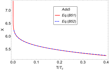
(a) $X$ vs $T/T_{c}$ at $\Delta=2$

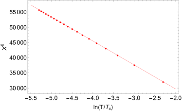
(b) $X^{6}$ vs $\log(T/T_{c})$ at $\Delta=2$.

Figure 25: (a) $X$ vs $T/T_{c}$: red colored curves for $X$ is a plot of Eq.(214). And blue curves is a plot of Eq.(215). These two curves are almost indentical for low temperature. (b)$X^{6}$ vs $\log(T/T_{c})$ at $\Delta=2$: The slope of red dotted line for $X^{6}$ is $-7900$.

B.2.3 Analytic calculation of $g^{\frac{1}{\Delta}}\frac{\left<\mathcal{O}_{\Delta}\right>^{\frac{1}{\Delta}}}{(g\rho)^{1/3}}$ at $1<\Delta<4$

Apply Eq.(207) into Eq.(208) with $T=\frac{1}{\pi}r_{h}$ with $b=\left(\frac{g\left<\mathcal{O}_{\Delta}\right>}{\Delta r_{h}^{\Delta}}\right)^{\frac{1}{\Delta}}$ in the form of $Y$; here, $Y:=$ $\frac{g^{1/\Delta}\left<\mathcal{O}_{\Delta}\right>^{1/\Delta}}{(g\rho)^{1/3}}$ for simple notation, we obtain the condensate at $T\approx 0$:

$$Y^{6}=\widetilde{G_{4}}^{6}\left(\alpha_{4}+\beta_{4}\widetilde{\tau_{4}}^{4-2\Delta}Y^{4-2\Delta}\right)$$ (216)

$$\hbox{where }\quad\widetilde{G_{4}} = \Delta^{1/\Delta}\left(\frac{-2^{1+\nu}}{\Gamma(-\nu)}\right)^{\frac{1}{3}}$$ (217)

$$\widetilde{\tau_{4}} = \frac{1}{\pi\Delta^{1/\Delta}}\frac{(g\rho)^{1/3}}{T}$$ (218)

with $\nu=\frac{1}{\Delta}$. Here, $\alpha_{4}$ and $\beta_{4}$ are in Eq.(210).

B.2.4 Analytic calculation of $g^{\frac{1}{\Delta}}\frac{\left<\mathcal{O}_{\Delta}\right>^{\frac{1}{\Delta}}}{(g\rho)^{1/3}}$ at $\Delta=2$

As Eq.(211) and Eq.(212) are substituted into Eq.(216) with taking the limit $\Delta\rightarrow 2$, we obtain

$$Y^{6}=\widetilde{G_{4}}^{6}\left(\rho_{4}+\frac{\sigma_{4}}{2}\left(\frac{1-\widetilde{\tau_{4}}^{4-2\Delta}Y^{4-2\Delta}}{\Delta-2}\right)\right).$$ (219)

By using L’Hopital’s rule, Eq.(219) becomes

$$Y^{6} = \widetilde{G_{4}}^{6}\left(\rho_{4}-\frac{\sigma_{4}}{2}\frac{\partial}{\partial\Delta}\left(\widetilde{\tau_{4}}^{4-2\Delta}Y^{4-2\Delta}\right)\right)$$ (220)

$$= \widetilde{G_{4}}^{6}\left(\rho_{4}+\sigma_{4}\ln\left(\widetilde{\tau_{4}}Y\right)\right)$$

Fig. 26 (b) tells us that $Y\sim\ln((g\rho)^{1/3}/T)^{1/6}$ for low temperature; Numerical result tells us that $Y^{6}$-$\log(T/(g\rho)^{1/3})$ plot demonstrates our arguements with high precision.

And $Y$ is numerically

$$Y \approx 0.89\left(1+4.23\ln\left(\frac{\sqrt{(}g\rho)^{1/3}}{T}\right)\right)^{1/6}$$ (221)

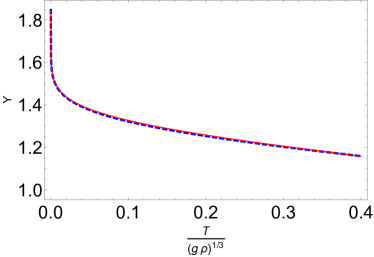
(a) $Y$ vs $T/(g\rho)^{1/3}$ at $\Delta=2$

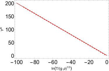
(b) $Y^{4}$-$\log(T/(g\rho)^{1/3})$ graph at $\Delta=2$.

Figure 26: (a) $Y$ vs $T/(g\rho)^{1/3}$: red colored curves for $Y$ is a plot of Eq.(220). And blue dashed curves is a plot of Eq.(221). These two curves are almost indentical for low temperature.
(b)$Y^{6}$-$\log(T/(g\rho)^{1/3})$ graph at $\Delta=2$: The slope of red dotted line for $Y^{6}$ is $-2$.

Appendix C Discussion

In this paper, we calculated the physical observables $T_{c},\langle{\cal O}_{\Delta}\rangle,\sigma({\omega}),\omega_{g},\omega_{i},n_{s},$ as functions of ${\mathcal{O}_{\Delta}},T,\rho$. Here we describe the main differences so that the readers understand the source of the differences in the results.

1. We use matrix algorithm by applying Pincherle’s Theorem to obtain the smallest value $\lambda_{g,3}$. On the other hand, The authors of ref. Siop2010 obtained the minimum value of $\lambda_{g,3}$’s by using variational method (see Eq.(40)) and they used the trial function $F(z)=1-\alpha z^{2}$. $F(z)$ does not converge on the boundary of the disc of convergence at $z=1$ in general. However, Pincherle’s Theorem tells us that $F(z)$ converges at $z=1$ for some quantized value of $\lambda_{g,3}$. As a consequence, our methodology works straightforwardly without ambiguity caused by the divergences and effective to get an eigenvalue when a power series is made up of three or more term recurrence relation. Notice also that our method shows that there is no well defined solution for $1/2<\Delta<1$ because of three branches of $\lambda_{g,3}$. But variational method do not show this phenomemon: Moreover, it tell us that there is $\lambda_{g,3}=0$ at $\Delta=1/2$ which is unphysical, since $\lambda_{g,3}=0$ means that $T_{c}$ is infinite.

2. The authors of ref. Siop2010 applied perturbation theory to obtain the condensate near $T_{c}$. It leads to the integral such as ${\cal C}_{3}=\int_{0}^{1}dz\;\frac{z^{2(\Delta-1)}F^{2}(z)}{z^{2}+z+1}$. Instead, we first obtain the analytic solution given by $F(z)=\left(z^{2}+z+1\right)^{-\frac{\lambda_{g,3}}{\sqrt{3}}}\sum_{n=0}^{15}d_{n}z^{n}$ (see Eq.(45)). Then we used it to evaluate Eq.(44). The result gives dramatic differences: For $\Delta=3$ in $d=3$, we have a finite result for ${\cal C}_{3}$, while they claimed they got ${\cal C}_{3}=0$. As a consequence, $g^{\frac{1}{\Delta}}\frac{\left<\mathcal{O}_{\Delta}\right>^{\frac{1}{\Delta}}}{T_{c}}$ is finite at $\Delta=3$ in our result, while they have divergent result.

3. Our the boundary condition of $F(z)$ and $\Phi(z)$ in AdS₄ is given in the following table.

   Over all the regime we consider, i.e, $\frac{1}{2}<\Delta<3$
   $(i)$ $F(0)=1$,  $\Phi^{{}^{\prime}}(0)=-{\rho}/{r_{h}}$
   $(ii)$ $\Phi(1)=0$ , $3F^{{}^{\prime}}(1)+\Delta^{2}F(1)=0$

   Table 6: Boundary condition of $F(z)$ and $\Phi(z)$ at the origin and the unity

   On the other hand, the authors of ref. Siop2010 used different boundary condition and different trial wave function according the regimes: $\frac{1}{2}<\Delta<\frac{3}{2}$ and $\frac{3}{2}<\Delta<{3}$. To compute Eq.(87a) and Eq.(87b), they applied $K_{\nu}(z)\sim\frac{\Gamma(\nu)}{2}\left(\frac{2}{z}\right)^{\nu}$ as $z\rightarrow 0$ into them. Because modified Bessel function $K$ is exponentially suppressed in large $z$. So they thought the dominant contribution comes from near $z=0$ region. Unfortunately, we cannot use near zero expression of $K_{\nu}$ inside the non-local double integral. In fact, using $K_{\nu}(z)\sim\frac{1}{z^{\nu}}$ in Eq.(87a) gives completely different result from using the full expression of $K_{\nu}(z)\sim\frac{e^{-z}}{\sqrt{z}}$, which we did here.

   Unlike in the case of $\frac{1}{2}<\Delta<\frac{3}{2}$, they used variational method without condition $3F^{{}^{\prime}}(1)+\Delta^{2}F(1)=0$ to compute $\mathcal{A}^{2}$ in Eq.(86) in the regime $\frac{3}{2}<\Delta<3$. They used different boundary condition at different region of $\Delta$. We believe that this is not necessary.

- (1) S. A. Hartnoll, C. P. Herzog and G. T. Horowitz, Building a holographic superconductor, Physical Review Letters 101 (2008) 031601, [0803.3295].
- (2) S. S. Gubser, Breaking an Abelian gauge symmetry near a black hole horizon, Phys.Rev. D78 (2008) 065034, [0801.2977].
- (3) S. A. Hartnoll, A. Lucas and S. Sachdev, Holographic quantum matter, 1612.07324.
- (4) J. M. Maldacena, The Large N limit of superconformal field theories and supergravity, Int.J.Theor.Phys. 38 (1999) 1113–1133, [hep-th/9711200].
- (5) E. Witten, Anti-de Sitter space and holography, Adv. Theor. Math. Phys. 2 (1998) 253–291, [hep-th/9802150].
- (6) S. S. Gubser, I. R. Klebanov and A. M. Polyakov, Gauge theory correlators from noncritical string theory, Phys. Lett. B428 (1998) 105–114, [hep-th/9802109].
- (7) G. T. Horowitz and M. M. Roberts, Holographic superconductors with various condensates, Physical Review D 78 (2008) 126008.
- (8) G. Siopsis and J. Therrien, Analytic calculation of properties of holographic superconductors, Journal of High Energy Physics 2010 (2010) 1–18.
- (9) G. Siopsis, Holographic superconductors at low temperatures, Bulletin of the American Physical Society 56 (2011) .
- (10) F. Denef and S. A. Hartnoll, Landscape of superconducting membranes, Physical Review D 79 (2009) 126008.
- (11) E. W. Leaver, Quasinormal modes of reissner-nordström black holes, Physical Review D 41 (1990) 2986.
- (12) M. N. Hounkonnou and A. Ronveaux, Generalized heun and lame’s equations: factorization, arXiv preprint arXiv:0902.2991 (2009) .
- (13) L. M. Milne-Thomson, The calculus of finite differences. American Mathematical Soc., 2000.
- (14) O. Perron, Über summengleichungen und poincarésche differenzengleichungen, Mathematische Annalen 84 (1921) 1–15.
- (15) H. Poincare, Sur les équations linéaires aux différentielles ordinaires et aux différences finies, American Journal of Mathematics (1885) 203–258.
- (16) W. B. Jones and W. J. Thron, Continued fractions: Analytic theory and applications, vol. 11. Addison-Wesley Publishing Company, 1980.
- (17) C. P. Herzog, Analytic holographic superconductor, Physical Review D 81 (2010) 126009.
- (18) X. Qiao, D. Wang, L. OuYang, M. Wang, Q. Pan and J. Jing, An analytic study on the excited states of holographic superconductors, Physics Letters B 811 (2020) 135864.
- (19) E. Mefford and G. T. Horowitz, Simple holographic insulator, Physical Review D 90 (2014) 084042.
- (20) R. Cai, L. Li, L. Li and R. Yang, Introduction to holographic superconductor models, Science China Physics, Mechanics & Astronomy 58 (2015) 1–46.
- (21) X.-H. Ge, B. Wang, S.-F. Wu and G.-H. Yang, Analytical study on holographic superconductors in external magnetic field, Journal of High Energy Physics 2010 (2010) 1–19.
- (22) S. Gangopadhyay and D. Roychowdhury, Analytic study of properties of holographic p-wave superconductors, Journal of High Energy Physics 2012 (2012) 1–12.
- (23) Q. Pan and B. Wang, General holographic superconductor models with gauss–bonnet corrections, Physics Letters B 693 (2010) 159–165.
- (24) R.-G. Cai, H.-F. Li and H.-Q. Zhang, Analytical studies on holographic insulator/superconductor phase transitions, Physical Review D 83 (2011) 126007.
- (25) J. Jing, Q. Pan and S. Chen, Holographic superconductors with power-maxwell field, Journal of High Energy Physics 2011 (2011) 1–12.
- (26) D. Roychowdhury, Effect of external magnetic field on holographic superconductors in presence of nonlinear corrections, Physical Review D 86 (2012) 106009.
- (27) S. Gangopadhyay and D. Roychowdhury, Analytic study of gauss-bonnet holographic superconductors in born-infeld electrodynamics, Journal of High Energy Physics 2012 (2012) 1–10.
- (28) H.-F. Li, R.-G. Cai and H.-Q. Zhang, Analytical studies on holographic superconductors in gauss-bonnet gravity, Journal of High Energy Physics 2011 (2011) 1–14.
- (29) Q. Pan, J. Jing and B. Wang, Analytical investigation of the phase transition between holographic insulator and superconductor in gauss-bonnet gravity, Journal of High Energy Physics 2011 (2011) 1–17.
- (30) H.-B. Zeng, X. Gao, Y. Jiang and H.-S. Zong, Analytical computation of critical exponents in several holographic superconductors, Journal of High Energy Physics 2011 (2011) 1–17.
- (31) R. Flauger, E. Pajer and S. Papanikolaou, Striped holographic superconductor, Physical Review D 83 (2011) 064009.
- (32) Z. Zhao, Q. Pan, S. Chen and J. Jing, Notes on holographic superconductor models with the nonlinear electrodynamics, Nuclear Physics B 871 (2013) 98–110.
- (33) Y. Liu, Q. Pan and B. Wang, Holographic superconductor developed in btz black hole background with backreactions, Physics Letters B 702 (2011) 94–99.
- (34) Z. Zhao, Q. Pan and J. Jing, Holographic insulator/superconductor phase transition with weyl corrections, Physics Letters B 719 (2013) 440–447.
- (35) D. Roychowdhury, Ads/cft superconductors with power maxwell electrodynamics: reminiscent of the meissner effect, Physics Letters B 718 (2013) 1089–1094.
- (36) S. Kanno, A note on gauss–bonnet holographic superconductors, Classical and Quantum Gravity 28 (2011) 127001.
- (37) Y. Peng, Q. Pan and B. Wang, Various types of phase transitions in the ads soliton background, Physics Letters B 699 (2011) 383–387.
- (38) Q. Pan, J. Jing, B. Wang and S. Chen, Analytical study on holographic superconductors with backreactions, Journal of High Energy Physics 2012 (2012) 1–12.
- (39) R. Banerjee, S. Gangopadhyay, D. Roychowdhury and A. Lala, Holographic s-wave condensate with nonlinear electrodynamics: A nontrivial boundary value problem, Physical Review D 87 (2013) 104001.
- (40) W. Yao and J. Jing, Analytical study on holographic superconductors for born-infeld electrodynamics in gauss-bonnet gravity with backreactions, Journal of High Energy Physics 2013 (2013) 1–16.
- (41) J.-W. Lu, Y.-B. Wu, P. Qian, Y.-Y. Zhao, X. Zhang and N. Zhang, Lifshitz scaling effects on holographic superconductors, Nuclear Physics B 887 (2014) 112–135.
- (42) A. Sheykhi, H. R. Salahi and A. Montakhab, Analytical and numerical study of gauss-bonnet holographic superconductors with power-maxwell field, Journal of High Energy Physics 2016 (2016) 1–17.
- (43) D. Ghorai and S. Gangopadhyay, Higher dimensional holographic superconductors in born–infeld electrodynamics with back-reaction, The European Physical Journal C 76 (2016) 1–12.
- (44) A. Sheykhi and F. Shaker, Analytical study of holographic superconductor in born–infeld electrodynamics with backreaction, Physics Letters B 754 (2016) 281–287.
- (45) C. Lai, Q. Pan, J. Jing and Y. Wang, On analytical study of holographic superconductors with born–infeld electrodynamics, Physics Letters B 749 (2015) 437–442.
- (46) Y. Liu, Q. Pan, B. Wang and R.-G. Cai, Dynamical perturbations and critical phenomena in gauss–bonnet ads black holes, Physics Letters B 693 (2010) 343–350.
- (47) J. Erdmenger, X.-H. Ge and D.-W. Pang, Striped phases in the holographic insulator/superconductor transition, Journal of High Energy Physics 2013 (2013) 1–29.
- (48) X.-M. Kuang, E. Papantonopoulos, G. Siopsis and B. Wang, Building a holographic superconductor with higher-derivative couplings, Physical Review D 88 (2013) 086008.
- (49) S. Gangopadhyay, Holographic superconductors in born–infeld electrodynamics and external magnetic field, Modern Physics Letters A 29 (2014) 1450088.
- (50) L. Zhang, Q. Pan and J. Jing, Holographic p-wave superconductor models with weyl corrections, Physics Letters B 743 (2015) 104–111.
- (51) R.-G. Cai, L. Li, H.-Q. Zhang and Y.-L. Zhang, Magnetic field effect on the phase transition in ads soliton spacetime, Physical Review D 84 (2011) 126008.
- (52) K.-Y. Kim and M. Taylor, Holographic d-wave superconductors, Journal of High Energy Physics 2013 (2013) 112.
- (53) W. Yao and J. Jing, Holographic entanglement entropy in metal/superconductor phase transition with born–infeld electrodynamics, Nuclear Physics B 889 (2014) 109–119.
- (54) G. T. Horowitz, Introduction to holographic superconductors, in From gravity to thermal gauge theories: the AdS/CFT correspondence, pp. 313–347. Springer, 2011.
- (55) I. S. Gradshteyn and I. M. Ryzhik, Table of integrals, series, and products. Academic press, 2014.
- (56) I. Thompson, Nist handbook of mathematical functions, edited by frank wj olver, daniel w. lozier, ronald f. boisvert, charles w. clark, 2011.
- (57) F. M. Arscott, S. Y. Slavyanov, D. Schmidt, G. Wolf, P. Maroni and A. Duval, Heun’s differential equations. Clarendon Press, 1995.
- (58) G. Siopsis, J. Therrien and S. Musiri, Holographic superconductors near the breitenlohner–freedman bound, Classical and Quantum Gravity 29 (2012) 085007.