Receding Horizon Iterative Learning Control for Continuously Operated Systems

Abstract

This paper presents an iterative learning control (ILC) scheme for continuously operated repetitive systems for which no initial condition reset exists. To accomplish this, we develop a lifted system representation that accounts for the effect of the initial conditions on dynamics and projects the dynamics over multiple future iterations. Additionally, we develop an economic cost function and update law that considers the performance over multiple iterations in the future, thus allowing for the prediction horizon to be larger than just the next iteration. Convergence of the iteration varying initial condition and applied input are proven and demonstrated using a simulated servo-positioning system test case.

I Introduction

For systems that exhibit repetitive behavior, repetitive and iterative learning control (ILC) techniques have proven to be useful tools that enable system performance to be improved through a learning-based update of the control signal. Traditionally, these strategies have aimed to eliminate tracking error of a known reference signal by leveraging information available in previous executions of a task to counteract uncertainties in the system. Typically, ILC has been developed for batch processes wherein the system undergoes an initial condition reset between iterations of the repetitive task. A common method of implementation of ILC controllers is depicted in the block diagram shown in Figure 1. Here, measurements of the system states and outputs, as well as knowledge of previously applied control signals, initial conditions, and reference signals, are utilized to design improved control signals in future iterations [1]. Meanwhile, repetitive control has generally been used for continuous processes where no such reset of the initial condition occurs between iterations [2].

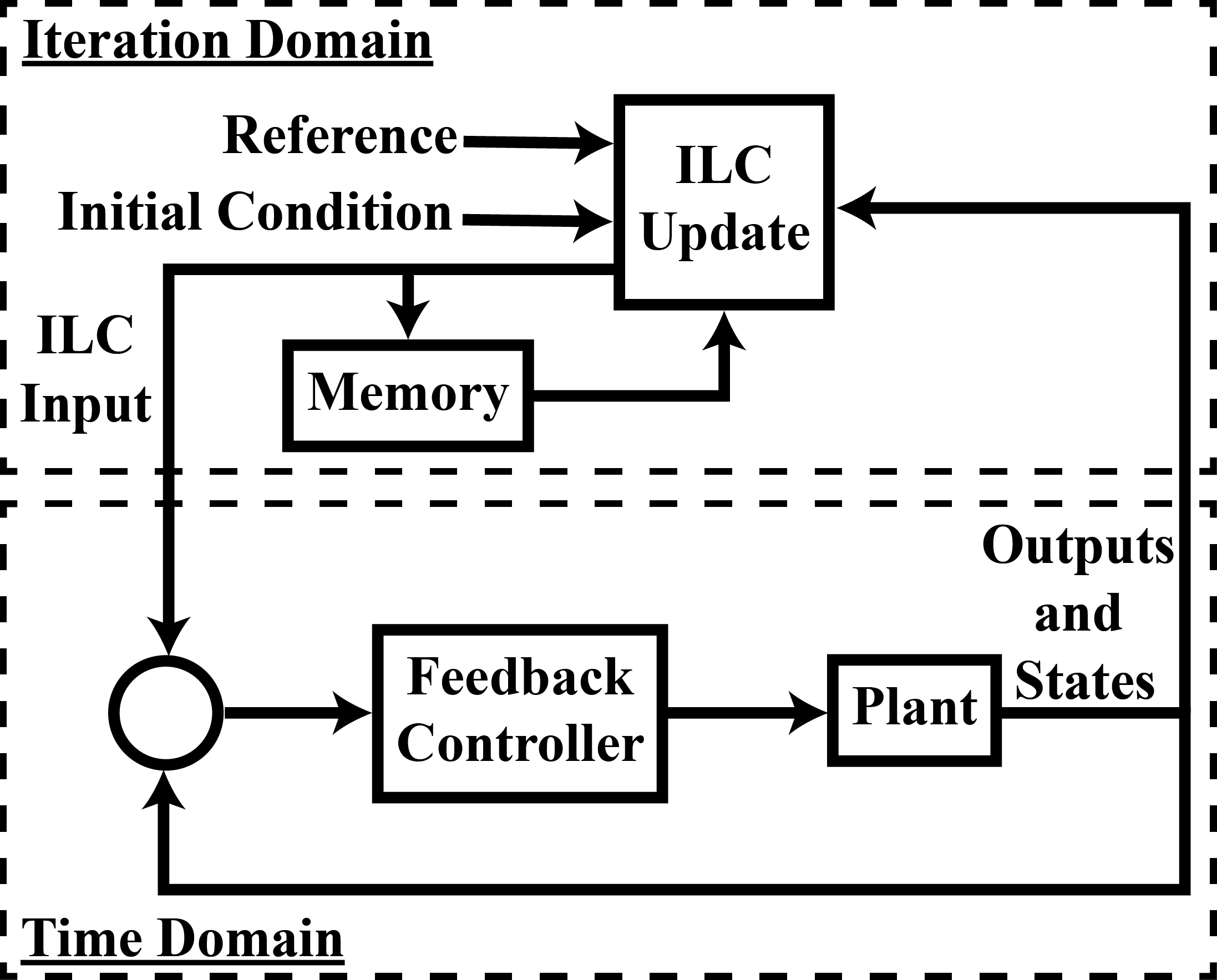
Figure 1: ILC utilizes iteration domain feedback to inform how a system is to be controlled in future iterations. An iteration-varying feedforward input signal aims to improve the behavior of the system by compensating for model uncertainties.

Many repetitive systems operate continuously. For instance, in autonomous racing applications the vehicle must repeatedly follow a predefined path with the goal of minimizing total lap time. Here, the control actions at a given lap will influence the behavior of the vehicle in future laps. Specifically, the system is considered continuously operable in that the initial condition at each iteration is given by the terminal condition at the previous iteration. Additionally, note that here the performance is not strictly dependent on the ability of the system to accurately track a predefined reference trajectory. Rather, the improved performance is achieved if the system is better able to minimize the non-traditional performance metric of lap time. These economic metrics enable system performance to be assessed for a broader range of systems such as robotic prosthetic legs that aim to follow a continuous gait trajectory while expending as little energy as possible, or tethered energy systems that follow a repetitive closed flight path with the primary objective of maximizing power generation.

Traditionally, repetitive control design has relied on a frequency domain analysis wherein the internal model principle is employed for the purpose of tracking periodic references or rejection of periodic disturbances [2]. However, while suitable for strict trajectory tracking objectives, controller design in the frequency domain is difficult to exercise when improvement in more general economic performance metrics is desired. On the other hand, ILC design has often leveraged state space models to improve system performance through iteration-based feedback. The use of state-space analysis has enabled the development of system representations in the lifted domain, as well as ‘norm-optimal’ controller design, which permits the intuitive construction of quadratic cost functions as a function of the control signal [3].

Historically, ILC designs have been made to minimize these cost functions by updating the feedforward control signal from data obtained in the previous iteration. While such strategies have proven useful, by only using information from a single iteration, these techniques neglect potential benefits to system performance that can be obtained by utilizing information from multiple iterations. To combat this, a subfield of ILC called ‘predictive iterative learning control’, as described in [4], [5], [6], [7], and [8], has been developed that not only uses information from the previous iteration, but also uses predictions of system behavior in future iterations to update the control signal. These strategies have shown improved convergence rates in comparison to traditional ILC while still establishing requirements for stability. However, these works consider a class of systems where the initial condition is reset between iterations.

To accommodate continuously operable systems, several techniques have been created. The strategy given by [9] and [10] iteratively updates safe sets over which system constraints are satisfied. A model predictive control optimization problem is then solved where the enlarged safe sets allow for a broader selection of control signals to be applied, thus giving opportunities for improved performance. This strategy has been previously used for the autonomous racing application described above and shown to be effective in reducing total lap time. However, this formulation dispenses with the ‘lifted system’ representation commonly used in ILC, as well as learning filters used to construct a closed form update law. In [11] and [12], a state-space based repetitive control strategy is designed to minimize performance of a system over an infinite prediction horizon by describing the problem as an iteration-domain LQ regulation problem with a control law given by solution of the algebraic Riccati equation. However, only the infinite horizon case is considered and no analysis giving requirements for stability or robustness to disturbances is given.

To address these issues, a receding horizon ILC formulation is developed for application to continuously operated systems. The contributions of this paper are given by

1. Generation of a lifted system representation that describes the impact of initial conditions and a multi-iteration control signal on the system dynamics.

2. A closed form update law that describes how the control signal is updated to reduce the value of a multi-iteration cost function.

3. An analysis of conditions for closed loop stability and desired system performance with considerations toward robustness to uncertain plant dynamics and disturbances.

4. Implementation of the algorithm to linear time-invariant and linear time varying systems.

II Receding Horizon Iterative Learning Control

The proposed ILC formulation contains two features that facilitate the consideration of continuous operation where an initial condition reset between cycles does not exist. This is achieved by combining a lifted system model that explicitly includes the impact of nonzero initial conditions with a performance index that includes predicted performance over multiple future iterations. Thus, the framework is capable of implicitly considering the impact of control decisions from one iteration on future iterations. The resulting iterative update law then provides control sequences for multiple future iterations. However, due to the need to adjust for disturbances and modeling uncertainties and inaccuracies, this feedforward control sequence is only applied one iteration at a time before being updated. The following subsections detail this approach.

III Controller Analysis

The stability properties and desired system behavior of the RHILC controller are now examined.

IV Illustrative Example: Servo-Positioning System

The RHILC algorithm is now implemented in simulation to a servo-positioning system described in [15]. To demonstrate the advantages of using a receding horizon approach to continuously operating systems, simulations are conducted on an iteration-invariant nominal model using the strategy described in Section LABEL:sec:MultiIterationSystemModel. Additionally, simulations on an iteration varying model with added uncertainty are presented to demonstrate the effectiveness of the algorithm in a more practical case.

V Conclusions

This paper proposes an ILC strategy for continuously operated systems in which the initial condition is not reset between iterations. A multi-iteration dynamic model is defined using a lifted system representation that describes the behavior of the system in response to multi-iteration input sequences and arbitrary initial conditions. A closed form, receding horizon style update law for the input sequence is presented, with stability criteria and desired performance standards established for time-invariant and time-varying systems.

The scheme is then implemented through simulation on a servo-positioning system where it is observed that improved system behavior can be achieved by utilizing a multi-iteration receding horizon approach in comparison to traditional ILC strategies. Additionally, the improved converged performance of the system when utilizing a finite prediction horizon length is established when modelling inaccuracies and disturbances are present.

Future work includes extensions towards systems with general convex cost functions and for which full state information is not known, and the use of constrained optimal control strategies with terminal components to ensure improved closed-loop performance. Additional work will also address non-linear systems and systems with spatially-defined dynamics.

VI Appendix

VI-A Performance Index Weighting Matrices

In (LABEL:eqn:longFormPerformance), the weighting matrices $Q_{u}$, $Q_{\delta u}$, $Q_{e}$, $Q_{x}$, and $Q_{\delta x}$, are easily defined in terms of three functions,

• the “diagonal” matrix function, $f_{D}\mathrel{\mathop{\mathchar 58\relax}}\mathbb{R}^{n_{a}}\mapsto\mathbb{R}^{n_{a}\times n_{a}}$ which takes in an input vector, $v=[v_{1},\,v_{2},\,\ldots,\,v_{n_{a}-1},\,v_{n_{a}}]$, and outputs a matrix with the entries of the input vector along the diagonal and zeros elsewhere.

  $$f_{D}(v)=\begin{bmatrix}v_{1}&0&\ldots&0&0\\ 0&v_{2}&\ldots&0&0\\ \vdots&\vdots&\ldots&\vdots&\vdots\\ 0&0&\ldots&v_{n_{a}-1}&0\\ 0&0&\ldots&0&v_{n_{a}-1}\\ \end{bmatrix}$$ (1)

• the “repeated block diagonal” matrix function, $f_{\Delta}\mathrel{\mathop{\mathchar 58\relax}}(n_{b},\mathbb{R}^{n_{c}\times n_{d}})\mapsto\mathbb{R}^{n_{b}n_{c}\times n_{b}n_{d}}$ which accepts the positive integer, $n_{b}$, and an arbitrary matrix, $C\in\mathbb{R}^{n_{c}\times n_{d}}$, and returns a block matrix with the input matrix repeated $n_{b}$ times along the block diagonal

  $$f_{\Delta}(n_{b},C)\triangleq\begin{bmatrix}C&\mathbb{0}&\ldots\\ \mathbb{0}&C&\ldots\\ \vdots&\vdots&\vdots\end{bmatrix}$$ (2)

If we then define the vectors of user-selected scalar weights as

$$\begin{split}q_{u}&\triangleq\begin{bmatrix}q_{u,1}&\ldots&q_{u,n_{u}}\end{bmatrix}^{T},\\ q_{\delta u}&\triangleq\begin{bmatrix}q_{\delta u,1}&\ldots&q_{\delta u,n_{u}}\end{bmatrix}^{T},\\ q_{e}&\triangleq\begin{bmatrix}q_{e,1}&\ldots&q_{e,n_{x}}\end{bmatrix}^{T},\\ q_{x}&\triangleq\begin{bmatrix}q_{x,1}&\ldots&q_{x,n_{x}}\end{bmatrix}^{T},\\ q_{\delta x}&\triangleq\begin{bmatrix}q_{\delta x,1}&\ldots&q_{\delta x,n_{x}}\end{bmatrix}^{T},\\ s_{x}&\triangleq\begin{bmatrix}s_{x,1}&\ldots&s_{x,n_{x}}\end{bmatrix}^{T}.\end{split}$$ (3)

Then the gain matrices $Q_{u}$, $Q_{\delta u}$, $Q_{e}$, $Q_{\delta e}$, $Q_{x}$ that encode the relative importance of each term in the performance index are given by

$$\begin{split}Q_{u}&=f_{\Delta}\left(n_{s},f_{D}(q_{u})\right),\\ Q_{\delta u}&=f_{\Delta}\left(n_{s},f_{D}(q_{\delta u})\right),\\ Q_{e}&=f_{\Delta}\left(n_{s},f_{D}(q_{e})\right),\\ Q_{x}&=f_{\Delta}\left(n_{s},f_{D}(q_{x})\right),\\ Q_{\delta x}&=f_{\Delta}\left(n_{s},f_{D}(q_{\delta x})\right).\end{split}$$ (4)

VI-B Cost and Constraint Matrices for Compact Optimization Problem

In (LABEL:Eq:_Compact_Optimization_Problem), the optimization problem is defined according to

$$\begin{split}\bm{\hat{\bar{Q}}}_{q}\triangleq&\bm{E}_{s}^{T}\left(\bm{I}_{u}^{T}\bm{\hat{Q}}_{u}\bm{I}_{u}-2\bm{Q}_{\delta u}\right)\bm{E}_{s}+\left(\stackunder[1.2pt]{$\bm{G}$}{\rule{3.44444pt}{0.32289pt}}\bm{E}_{s}+\stackunder[1.2pt]{$\bm{F}$}{\rule{3.44444pt}{0.32289pt}}\bm{E}_{e}\right)^{T}...\\ &\left(\bm{I}_{x}^{T}(\bm{\hat{Q}}_{x}+\bm{\hat{Q}}_{e})\bm{I}_{x}-2\bm{Q}_{\delta x}\right)\left(\stackunder[1.2pt]{$\bm{G}$}{\rule{3.44444pt}{0.32289pt}}\bm{E}_{s}+\stackunder[1.2pt]{$\bm{F}$}{\rule{3.44444pt}{0.32289pt}}\bm{E}_{e}\right)\\ \bm{\hat{\bar{q}}}_{l}\triangleq&(\stackunder[1.2pt]{$\bm{G}$}{\rule{3.44444pt}{0.32289pt}}\bm{E}_{s}+\stackunder[1.2pt]{$\bm{F}$}{\rule{3.44444pt}{0.32289pt}}\bm{E}_{e})^{T}\Big{(}\bm{I}_{x}^{T}(\bm{\hat{Q}}_{x}+\bm{\hat{Q}}_{e})\bm{I}_{x}\stackunder[1.2pt]{$d$}{\rule{3.44444pt}{0.32289pt}}...\\ &+\bm{I}_{x}^{T}(\bm{s}_{x}-\bm{\hat{Q}}_{e}\bm{I}_{x}\stackunder[1.2pt]{$r$}{\rule{3.44444pt}{0.32289pt}})-2\bm{Q}_{\delta x}\stackunder[1.2pt]{$d$}{\rule{3.44444pt}{0.32289pt}}\Big{)}\\ \mathbf{W}\triangleq&\bm{E}_{e}-\bm{E_{F}}(\stackunder[1.2pt]{$\bm{G}$}{\rule{3.44444pt}{0.32289pt}}\bm{E}_{s}+\stackunder[1.2pt]{$\bm{F}$}{\rule{3.44444pt}{0.32289pt}}\bm{E}_{e})\\ \mathbf{v}\triangleq&\bm{E_{F}}\stackunder[1.2pt]{$d$}{\rule{3.44444pt}{0.32289pt}}\end{split}.$$ (5)

VII Acknowledgements

This work was funded by National Science Foundation grant numbers 1727371 and 1727779 entitled “Collaborative Research: An Economic Iterative Learning Control Framework with Application to Airborne Wind Energy Harvesting.”

References

- [1] D. A. Bristow, M. Tharayil, and A. G. Alleyne, “A survey of iterative learning control,” IEEE Control Systems Magazine, vol. 26, no. 3, pp. 96–114, 2006.
- [2] Y. Wang, F. Gao, and F. J. Doyle, “Survey on iterative learning control, repetitive control, and run-to-run control,” Journal of Process Control, vol. 19, no. 10, pp. 1589 – 1600, 2009. [Online]. Available: http://www.sciencedirect.com/science/article/pii/S0959152409001681
- [3] S. Gunnarsson and M. Norrlöf, “On the design of ilc algorithms using optimization,” Automatica, vol. 37, no. 12, pp. 2011–2016, 2001.
- [4] B. Chu, D. H. Owens, and C. T. Freeman, “Iterative learning control with predictive trial information: Convergence, robustness, and experimental verification,” IEEE Transactions on Control Systems Technology, vol. 24, no. 3, pp. 1101–1108, 2016.
- [5] L. Wang and E. Rogers, “Predictive iterative learning control using laguerre functions,” IFAC Proceedings Volumes, vol. 44, no. 1, pp. 5747 – 5752, 2011, 18th IFAC World Congress. [Online]. Available: http://www.sciencedirect.com/science/article/pii/S1474667016445234
- [6] N. Amann, D. H. Owens, and E. Rogers, “Predictive optimal iterative learning control,” International Journal of Control, vol. 69, no. 2, pp. 203–226, 1998. [Online]. Available: https://doi.org/10.1080/002071798222794
- [7] M. Arif, T. Ishihara, and H. Inooka, “Prediction-based iterative learning control (pilc) for uncertain dynamic nonlinear systems using system identification technique,” Journal of Intelligent and Robotic Systems, vol. 27, no. 3, pp. 291–304, Mar 2000. [Online]. Available: https://doi.org/10.1023/A:1008162421594
- [8] B. Chu, D. H. Owens, and C. T. Freeman, “Predictive gradient iterative learning control,” in 2015 54th IEEE Conference on Decision and Control (CDC), 2015, pp. 2377–2382.
- [9] U. Rosolina, A. Carvhalo, and F. Borrelli, “Autonomous racing using learning model predictive control,” Proceedings of the 2017 IFAC World Congress, 2017, Toulouse, France.
- [10] M. Brunner, R. Ugo, J. Gonzales, and F. Borelli, “Repetitive learning model predictive control: An autonomous racing example,” Proceedings of the 56th Conference on Decision and Control, 2017, Melbourne, Australia.
- [11] J. H. Lee, S. Natarajan, and K. S. Lee, “A model-based predictive control approach to repetitive control of continuous processes with periodic operations,” Journal of Process Control, vol. 11, no. 2, pp. 195 – 207, 2001. [Online]. Available: http://www.sciencedirect.com/science/article/pii/S0959152400000470
- [12] M. Gupta and J. H. Lee, “Period-robust repetitive model predictive control,” Journal of Process Control, vol. 16, no. 6, pp. 545 – 555, 2006. [Online]. Available: http://www.sciencedirect.com/science/article/pii/S0959152406000035
- [13] I. Lim and K. Barton, “Pareto optimization-based iterative learning control,” Proceedings of the American Control Conference, 2013, Washington, D.C.
- [14] D. Clarke, C. Mohtadi, and P. Tuffs, “Generalized predictive control—part i. the basic algorithm,” Automatica, vol. 23, no. 2, pp. 137 – 148, 1987. [Online]. Available: http://www.sciencedirect.com/science/article/pii/0005109887900872
- [15] D. A. Bristow, K. L. Barton, A. G. Alleyne, and W. S. Levine, “Iterative learning control,” The Control Systems Handbook: Control System Advanced Methods, pp. 1–19, 2010.