Discovery of a New Population of Galactic H ii Regions with Ionized Gas Velocity Gradients

Abstract

We investigate the kinematic properties of Galactic H ii regions using radio recombination line (RRL) emission detected by the Australia Telescope Compact Array (ATCA) at 4–10$\,{\rm GHz}$ and the Jansky Very Large Array (VLA) at 8–10$\,{\rm GHz}$. Our H ii region sample consists of 425 independent observations of 374 nebulae that are relatively well isolated from other, potentially confusing sources and have a single RRL component with a high signal-to-noise ratio. We perform Gaussian fits to the RRL emission in position-position-velocity data cubes and discover velocity gradients in 178 (42%) of the nebulae with magnitudes between 5 and 200$\,{\rm m\,s^{-1}\,arcsec^{-1}}$. About 15% of the sources also have a RRL width spatial distribution that peaks toward the center of the nebula. The velocity gradient position angles appear to be random on the sky with no favored orientation with respect to the Galactic Plane. We craft H ii region simulations that include bipolar outflows or solid body rotational motions to explain the observed velocity gradients. The simulations favor solid body rotation since, unlike the bipolar outflow kinematic models, they are able to produce both the large, $>40$$\,{\rm m\,s^{-1}\,arcsec^{-1}}$, velocity gradients and also the RRL width structure that we observe in some sources. The bipolar outflow model, however, cannot be ruled out as a possible explanation for the observed velocity gradients for many sources in our sample. We nevertheless suggest that most H ii region complexes are rotating and may have inherited angular momentum from their parent molecular clouds.

1 Introduction

H ii regions are the zones of ionized gas surrounding young, OB-type stars. Feedback from these massive stars is an important mechanism in galaxy formation and evolution (e.g., Veilleux et al., 2005). For example, high-mass stars can produce radiation-driven outflows that both inhibit and stimulate star formation in their vicinities (e.g., Ali et al., 2018). Furthermore, the internal motions of H ii regions constrain models of star formation and evolution (e.g., Dalgleish et al., 2018). For example, high frequency RRLs that probe the high density gas within the ultra-compact H ii region G10.6$-$0.4 support evidence of an ionized accretion flow (Keto & Wood, 2006). RRL observations toward K3-50 reveal a velocity gradient across the nebula. This together with a bipolar morphology from the radio continuum emission indicates that this source is undergoing a high-velocity bipolar outflow (De Pree et al., 1994; Balser et al., 2001). RRL position-velocity diagrams of NGC 6334A reveal both a bipolar outflow and rotation in the ionized gas (De Pree et al., 1995; Balser et al., 2001). There is evidence that high-mass stars form in binaries or multiple star systems more often than low-mass stars (Mermilliod & García, 2001; Okamoto et al., 2003), creating massive accretion flows that overcome radiation and thermal pressure (Keto & Wood, 2006). Therefore H ii region bipolar outflows may arise from multiple OB-type stars. Most H ii region studies of this type, however, focus on one or a few sources. To our knowledge there have not been any surveys of the kinematic motions within H ii regions for a large number of sources.

H ii regions occupy intermediate spatial scales between giant molecular cloud (GMC) star forming complexes and individual protostars, both of which have a rich literature of kinematics studies. For example, on the large—tens of parsecs—scale both H i and CO tracers have been used to explore the angular momentum in the largest star forming structures (e.g., Fleck & Clark, 1981; Arquilla & Goldsmith, 1985; Imara & Blitz, 2011). The kinematic structure of molecular cores and protostars which probe the small—$\lesssim 0.05$$\,{\rm pc}$—scale have been investigated using dense molecular gas tracers (e.g., Goodman et al., 1993; Caselli et al., 2002; Chen et al., 2007; Tobin et al., 2011). Young, ultra-compact H ii regions have similar spatial scales with sizes less than 0.1$\,{\rm pc}$ (e.g., Churchwell, 2002). But over time the warm, $10^{4}$$\,{\rm K}$, plasma causes the H ii region to expand creating a “classical” H ii region that can span several parsecs, filling in the gap between GMCs and protostars. Photo-dissociation regions can also be exploited to probe the kinematics on these spatial scales (e.g., Luisi et al., 2021).

The lack of H ii region kinematic surveys is in part due to limitations of the available instrumentation of past facilities. Optical observations of H$\alpha$ typically have the necessary sensitivity and spatial resolution but often lack the spectral resolution needed for detailed kinematic studies. There are some exceptions (e.g., see Russeil et al., 2016). There are some extragalactic studies of H ii region kinematics, but they typically do not have the angular resolution to probe individual star formation regions (e.g., see Bordalo et al., 2009; Torres-Flores et al., 2013; Bresolin et al., 2020). Since H$\alpha$ emission is attenuated by dust the entire volume of ionized gas is not always sampled, therefore limiting the usefulness of this tracer. Fine structure lines at infrared wavelengths can penetrate the dust. For example, N ii 122µm (Lebouteiller et al., 2012) and Ne ii 12.8µm (Jaffe et al., 2005; Zhu, 2006) trace the dense ionized gas found in H ii regions. To our knowledge, however, there have not been any infrared studies of the kinematics for a large sample of H ii regions. In contrast, RRLs are optically thin tracers with sufficient spectral resolution, but they are often observed using single-dish telescopes with poor angular resolution. Radio interferometers can significantly improve the angular resolution but they are typically not sensitive to the more diffuse emission that exists in many H ii regions. Here we use RRL data from two new interferometer surveys that mitigate some of these weaknesses to investigate H ii region kinematics from a large sample of nebulae.

2 The Data

Data are taken from two recent H ii region RRL surveys: the Southern H ii Region Discovery Survey (SHRDS) using the ATCA (Wenger et al., 2021), and the H ii region VLA RRL survey (Wenger et al., 2019a). As the first H ii region RRL surveys using interferometer observations toward a large number of sources, they have sufficient spatial resolution to at least partially resolve many Galactic H ii regions. Moreover, the flexibility of their spectrometers allows many RRLs to be simultaneously observed and averaged together to increase the signal-to-noise ratio (e.g., Balser, 2006). Therefore, for the first time we have H ii region RRL surveys that have both the sensitivity and spatial resolution at radio wavelengths to measure the internal H ii region kinematics in a large sample. Table 1 summarizes the statistics for these surveys. Because each interferometer field may contain multiple H ii regions, we detect RRL and continuum emission from more H ii regions than are targeted and also have some duplicate observations.

Table 1: H ii Region Survey Statistics

Statistic	ATCA	VLA	Total	Comment
$N_{\rm tot}$	965 (669)	118 (117)	1083 (786)	Total number of sources in the survey.
$N_{\rm kin}$	377 (327)	48 (47)	425 (374)	Number of sources suitable for kinematic analysis.
$N_{\rm grad}$	166 (150)	12 (12)	178 (162)	Number of sources with a velocity gradient.
$f_{\rm grad}$	44 (46)	25 (26)	42 (43)	Percentage of suitable sources with a velocity gradient: $N_{\rm grad}/N_{\rm kin}$.

Note. — Counts correspond to independent detections toward the ATCA and VLA images. Since each image may contain multiple H ii regions there are some duplicate observations. In parentheses we list the unique source counts.

2.1 Australia Telescope Compact Array

The SHRDS is an ATCA 4–10$\,{\rm GHz}$ radio continuum and RRL survey to find H ii regions in the Galactic zone $259\,^{\circ}<\ell<344\,^{\circ},|b|<4\,^{\circ}$ (Brown et al., 2017; Wenger et al., 2019b, 2021). The SHRDS is an extension of the HRDS in the northern sky that used the Green Bank Telescope (GBT) and also the Arecibo telescope to observe H ii region candidates selected from public infrared and radio continuum data (Bania et al., 2010; Anderson et al., 2011; Bania et al., 2012; Anderson et al., 2015, 2018). These recent H ii region RRL surveys have doubled the number of known H ii regions in the Milky Way. The SHRDS full catalog consists of 436 new Galactic H ii regions and 206 previously known nebulae (Wenger et al., 2021). Here we consider every continuum detection in the SHRDS images for our initial analysis. This consists of 965 independent continuum measurements.

Since the ATCA is a compact array, the short baselines are better able to recover emission from the extended parts of an H ii region. The SHRDS employed the most compact antenna configuration, H75, together with the larger H168 configuration to probe a range of spatial scales. Moreover, the observations were made at different hour angles to provide good coverage in the uv-plane (see Figure 3 in Wenger et al., 2019b). The half-power beam-width (HPBW) spatial resolution is $\sim 90$″ and the maximum recoverable scale is $\sim 265$″. The ATCA Compact Array Broadband Backend (CABB) can tune simultaneously to 20 different RRLs across the 4–10$\,{\rm GHz}$ band. Typically, about 18 RRL transitions between H88$\alpha$–H112$\alpha$ were suitable to average together (stack) to produce a final spectrum, $\langle{\rm Hn}\alpha\rangle$. To do this we first re-grid the smoothed RRL data cubes to a common spectral and angular resolution, and then average the smoothed, regridded data cubes.

We select sources from the SHRDS that have the following criteria. (1) They must be either well isolated or only slightly confused, with a single continuum emission peak. All sources with quality factor A or B meet this criterion (see Wenger et al., 2021). (2) Spectra toward some H ii regions contain multiple RRL components which may be due to more than one distinct H ii region. So we restrict our analysis to sources with only single RRL components. (3) We require good sensitivity to infer kinematic structure across the H ii region. Therefore we only select sources with a peak RRL signal-to-noise ratio, ${\rm SNR}\geq 10$. Applying these criteria to the SHRDS yields 377 independent observations of 327 unique sources for kinematic analysis.

The SHRDS provides a very coarse measure of the kinematic structure in H ii regions. Most nebulae are resolved with only a few synthesized beams across the detected nebula emission. By design the ATCA observations, taken in the most compact configurations, do not provide very detailed images; the synthesized beam is not significantly smaller than the primary beam (HPBW = 225″). This is because for the SHRDS science goals surface brightness sensitivity is more important than spatial resolution. Nevertheless, here we will show that the sensitivity and spatial resolution are sufficient to roughly characterize the global properties of the internal kinematics of H ii regions.

2.2 Jansky Very Large Array

The goal of the H ii region VLA 8–10$\,{\rm GHz}$ RRL survey was to measure the metallicity throughout the Galactic disk in the northern sky (Wenger et al., 2019a). Accurate electron temperatures were derived using the RRL to continuum intensity ratio. Since metals act as coolants within the ionized gas, the electron temperatures are a proxy for metallicity (Rubin, 1985). A total of 82 nebulae were targeted. Multiple sources were sometimes detected within the primary beam and therefore here we consider every continuum detection in the VLA images. This consists of 118 independent continuum measurements.

Data were taken in the most compact VLA D configuration using $\sim 10$ minute “snapshot” integrations. The uv-plane was therefore not well sampled and the resulting RRL images are not very sensitive to any extended H ii region emission. The HPBW spatial resolution is 15″ and the maximum recoverable scale is 145″. The Wideband Interferometric Digital ARchitecture (WIDAR) correlator in the 8-bit sampler mode can tune simultaneously to 8 RRL transitions between H86$\alpha$–H93$\alpha$ across the 8–10$\,{\rm GHz}$ band. Since the H86$\alpha$ transition is confused with a higher order RRL only 7 RRLs are stacked to produce the $\langle{\rm Hn}\alpha\rangle$ spectrum.

We follow the same selection criteria as discussed in Section 2.1 for our kinematic analysis. We therefore only choose relatively isolated nebulae that have a single RRL component with a ${\rm SNR}\geq 10$. A total of 48 independent observations of 47 unique sources meet these criteria.

3 H ii Region Kinematics

Random gas motions of the plasma produced by photoionziation within H ii regions should be well described by a Maxwell-Boltzmann distribution. Such motions produce Gaussian spectral line profiles for optically thin gas via the Doppler effect. There is some evidence for small deviations from a Maxwell-Boltzmann distribution in H ii regions (e.g., Nicholls et al., 2012), but this should not significantly affect our interpretation of H ii region kinematics. Observations of spectral lines from ionized gas tracers indicate line widths significantly broader than the thermal width, even on small spatial scales (Ferland, 2001; Beckman & Relaño, 2004). These non-thermal line widths have been attributed to MHD waves (e.g., Mouschovias, 1975) or turbulence (e.g., Morris et al., 1974) which also produce Gaussian line profiles via the Doppler effect. Bulk motions of the gas produced by dynamical effects may alter the line shape. For example, an expanding H ii region could produce a double-peaked RRL profile if the nebula is resolved, or a square-wave RRL profile for an unresolved source (e.g., Balser et al., 1997). But analysis of $\langle{\rm Hn}\alpha\rangle$ spectra toward nebulae in the ATCA and VLA surveys typically reveal a single Gaussian line profile. There are six nebulae (3%) with significant non-Gaussian line wings or double-peaked profiles that are not included in our analysis.

To investigate the H ii region kinematics, we therefore perform single component, Gaussian fits to $\langle{\rm Hn}\alpha\rangle$ profiles for each spectral pixel (spaxel) in the RRL data cubes using the Levenberg-Markwardt (Markwardt, 2009) least-squares method. Figures 1 and 2 show the results of these fits for G297.651$-$00.973 and G035.126$-$0.755 taken from the ATCA and VLA surveys, respectively. Plotted are the fitted center velocity, $V_{\rm LSR}$, the full-width at half-maximum (FWHM) line width, $\Delta V$, and their associated errors. The $V_{\rm LSR}$ and $\Delta V$ images are similar to first and second moment maps, respectively, but in detail they are different mathematical operations. Figures 1–2 reveal clear velocity gradients across the roughly circular nebulae. G297.651$-$00.973 and G035.126$-$0.755 illustrate particularly good examples, but we detect velocity gradients in 44% and 25% of H ii regions in the ATCA and VLA surveys, respectively. Less common, however, is the centrally-peaked distribution of the FWHM line width detected in G297.651$-$00.973 and G035.126$-$0.755.

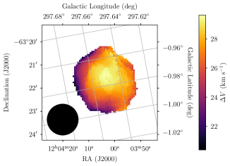
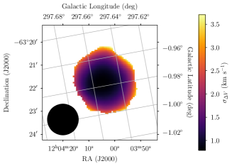
Figure 1: $\langle{\rm Hn}\alpha\rangle$ spectrum RRL Gaussian center velocity, $V_{\rm LSR}$, and line width, $\Delta V$, parameter images of G297.651$-$00.973, observed with the ATCA. Top: Gaussian fit of the center velocity, $V_{\rm LSR}$, and the associated error. Bottom: Gaussian fit of the FWHM line width, $\Delta V$, and the associated error. The boundaries of the fitted region are defined by a watershed segmentation algorithm that identifies all pixels with emission associated with an emission peak (for details see Wenger et al., 2021). Outside the watershed region the images have a poor signal-to-noise ratio and there are no Gaussian RRL fits. The synthesized HPBW is shown by the black circle in the bottom left-hand corner of the image.

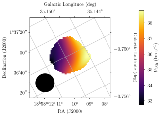
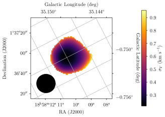
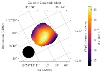
Figure 2: $\langle{\rm Hn}\alpha\rangle$ spectrum RRL Gaussian center velocity, $V_{\rm LSR}$, and line width, $\Delta V$, parameter images of G035.126$-$0.755 observed with the VLA. See Figure 1 for details.

To characterize the velocity gradients in our H ii region sample, we fit both a constant model (no velocity gradient) and a plane model (velocity gradient) to the $V_{\rm LSR}$ image using maximum likelihood estimation (MLE)—see Appendix A for details. For each model, we calculate the Bayesian Information Criterion (BIC). The BIC is used to select the best model that does not overfit the data. If $\Delta{\rm BIC}\equiv{\rm BIC(constant)}-\rm{BIC(plane)}\geq 6$ then the plane model is strongly preferred (Kass & Raftery, 1995). A total of 212 and 19 detections are best fit by a plane model for the ATCA and VLA, respectively. Visual inspection of both the Gaussian fit images and the data cubes for all sources with $\Delta{\rm BIC}\geq 6$ reveals problems with the velocity gradient fit for 46 and 7 detections for the ATCA and VLA, respectively. For example, the velocity gradient was either fit across two distinct sources or the source was cutoff by the primary beam. Removing these sources leaves a total of 166 and 12 nebulae with bona fide velocity gradients for the ATCA and VLA, respectively. Finally, to provide a quantitative measure of the goodness of fit we calculate the root mean square error (RMSE) between the model and data.

Tables 2 and 3 summarize the properties of our velocity gradient H ii regions for the ATCA and VLA, respectively. Listed are the source name, the source field, the MLE velocity gradient fit parameters, the quality factor, QF, the number of synthesized beams across the nebula, the RRL peak SNR, and the RMSE. The velocity gradient fit parameters consist of the velocity offset, $c_{0}$, the velocity gradient magnitude, $\nabla V_{\rm LSR}$, and the position angle, PA. The ATCA primary beam is large and often contains multiple H ii regions. Therefore, we have observed some sources multiple times in the SHRDS and these duplicates, consisting of 16 H ii regions, are included in Table 2 because they are independent measurements. They can be distinguished by the different field names.

The distribution of velocity gradient magnitudes and position angles are shown in Figure 3. Only unique sources with RMSE values less than 1.0$\,{\rm km\,s^{-1}}$ are included. Based on visual inspection of the $V_{\rm LSR}$ images and the velocity gradient fits, we deem that sources with RMSE less than 1.0$\,{\rm km\,s^{-1}}$ are well characterized by velocity gradients. Using this threshold for the RMSE excludes 74 and 5 detections from the ATCA and VLA H ii region sample, respectively. The ATCA H ii region sample velocity gradient magnitudes range between $\nabla V_{\rm LSR}=5-80$$\,{\rm m\,s^{-1}\,arcsec^{-1}}$, whereas the VLA H ii region sample have higher values, $\nabla V_{\rm LSR}=80-200$$\,{\rm m\,s^{-1}\,arcsec^{-1}}$. Since the VLA spatial resolution is about 10 times better than the ATCA we are not necessarily comparing the same area of the H ii region; this, of course, depends on the distance. Calculating the velocity gradient in physical units, $\,{\rm km\,s^{-1}\,pc^{-1}}$, may provide more stringent constraints on dynamical models, but here we decide to use the distance independent units of $\,{\rm m\,s^{-1}\,arcsec^{-1}}$ since we do not yet have accurate distances to many of our sources. The number of nebulae deceases with increasing velocity gradient magnitude and turns over near $\nabla V_{\rm LSR}=15$$\,{\rm m\,s^{-1}\,arcsec^{-1}}$. There are likely H ii regions with velocity gradients less than this value that we do not detect due to sensitivity.

Table 2: ATCA H ii Region Sample

		MLE Velocity Gradient Fit
		$c_{0}$	$\nabla V_{\rm LSR}$	PA		No.	Peak	RMSE
Source	Field	($\,{\rm km\,s^{-1}}$)	($\,{\rm m\,s^{-1}\,arcsec^{-1}}$)	(degree)	QF	Beams	SNR	($\,{\rm km\,s^{-1}}$)
G012.804$-$00.207	g012.804$-$	$35.65\pm 0.07$	$8.53\pm 0.84$	$265.26\pm 7.34$	A	3.6	281.00	0.74
G013.880+00.285	overlap4	$50.76\pm 0.04$	$14.94\pm 0.70$	$179.79\pm 3.02$	A	3.8	449.70	0.58
G233.753$-$00.193	ch1	$37.45\pm 0.30$	$41.93\pm 3.92$	$89.01\pm 6.08$	A	2.1	20.10	1.86
G259.057$-$01.544	shrds030	$59.18\pm 0.51$	$317.62\pm 18.12$	$126.50\pm 3.12$	A	1.0	25.40	9.12
G263.615$-$00.534	ch5	$0.08\pm 0.08$	$21.73\pm 2.06$	$155.71\pm 5.53$	A	5.3	91.80	1.03
G264.343+01.457	ch6	$13.27\pm 0.09$	$36.50\pm 2.64$	$40.66\pm 4.07$	A	4.1	98.00	0.69
G265.151+01.454	ch7	$6.03\pm 0.02$	$71.23\pm 0.73$	$74.12\pm 0.53$	A	8.3	218.20	4.21
G281.175$-$01.645	ch17	$-6.98\pm 0.13$	$14.54\pm 3.69$	$49.56\pm 14.21$	A	3.3	87.60	0.59
G281.175$-$01.645	caswell1	$-7.43\pm 0.18$	$15.74\pm 4.16$	$19.90\pm 15.79$	A	2.8	58.90	0.64
G282.015$-$00.997	shrds1007	$0.29\pm 0.13$	$26.61\pm 1.76$	$124.47\pm 3.63$	B	3.8	40.60	0.82
G282.027$-$01.182	ch19	$21.20\pm 0.06$	$31.29\pm 1.15$	$335.36\pm 2.35$	A	6.8	286.60	3.34
G282.842$-$01.252	shrds1232	$-4.61\pm 0.23$	$16.16\pm 4.75$	$281.33\pm 17.58$	A	2.4	36.50	1.17
G284.712+00.317	caswell2	$9.26\pm 0.12$	$39.98\pm 2.51$	$237.68\pm 3.64$	A	4.5	83.80	1.05
G284.712+00.317	ch32	$10.91\pm 0.11$	$48.64\pm 2.28$	$242.35\pm 2.85$	A	5.6	118.30	1.38
G285.260$-$00.051	ch33	$-1.02\pm 0.06$	$26.37\pm 1.11$	$177.09\pm 1.62$	A	7.6	229.70	1.50
G286.362$-$00.297	shrds1017	$-33.68\pm 0.19$	$52.57\pm 3.25$	$190.91\pm 3.98$	B	3.3	34.20	0.83
G286.362$-$00.297	shrds1018g	$-39.76\pm 0.27$	$49.51\pm 3.16$	$200.64\pm 2.79$	B	1.9	17.70	0.48
G286.391$-$01.351	ch35	$38.27\pm 0.18$	$34.71\pm 5.35$	$5.18\pm 6.16$	A	2.6	64.10	0.79
G291.046$-$02.079	shrds199	$-18.93\pm 0.19$	$37.70\pm 3.68$	$227.54\pm 5.59$	A	3.1	40.20	0.48
G291.281$-$00.726	caswell3	$-23.38\pm 0.07$	$46.15\pm 1.39$	$159.23\pm 1.65$	A	4.9	226.70	0.86
G291.281$-$00.726	ch52	$-23.58\pm 0.06$	$64.87\pm 1.29$	$163.43\pm 0.89$	A	6.3	407.40	1.24
G291.863$-$00.682	ch55	$24.92\pm 0.08$	$12.92\pm 1.78$	$329.46\pm 9.20$	A	4.5	144.60	0.91
G291.863$-$00.682	caswell4	$24.31\pm 0.10$	$9.71\pm 2.09$	$317.15\pm 12.31$	A	3.9	122.60	0.54
G293.024$-$01.029	ch57	$65.77\pm 0.15$	$19.83\pm 3.98$	$132.85\pm 11.51$	A	3.8	65.40	0.68
G293.967$-$00.984	shrds219	$28.46\pm 0.50$	$36.56\pm 12.10$	$83.34\pm 16.46$	B	1.1	28.20	0.38
G297.651$-$00.973	ch65	$31.76\pm 0.22$	$67.50\pm 5.91$	$94.55\pm 5.09$	A	2.9	46.50	0.71
G298.183$-$00.784	caswell5	$17.97\pm 0.12$	$13.18\pm 3.05$	$323.02\pm 13.28$	A	3.1	131.80	0.66
G298.183$-$00.784	ch66	$17.63\pm 0.12$	$11.14\pm 3.40$	$280.26\pm 18.76$	A	3.1	165.50	0.93
G298.224$-$00.334	ch67	$31.79\pm 0.07$	$60.01\pm 1.18$	$36.16\pm 1.25$	A	5.6	349.80	3.06
G298.846+00.121	shrds258	$19.65\pm 0.29$	$29.72\pm 5.80$	$111.24\pm 10.90$	A	1.5	38.60	0.47
G299.349$-$00.267	ch71	$-39.61\pm 0.20$	$16.16\pm 2.85$	$350.31\pm 8.49$	B	2.4	38.00	0.54
G299.349$-$00.267	caswell6	$-40.35\pm 0.18$	$24.88\pm 3.62$	$331.40\pm 8.18$	A	3.0	38.80	0.42
G300.965+01.162	g300.983+01.117	$-40.93\pm 0.16$	$30.18\pm 1.13$	$186.87\pm 4.41$	B	3.4	49.00	1.54
G301.116+00.968	caswell8	$-40.76\pm 0.08$	$41.28\pm 1.62$	$217.31\pm 2.22$	A	4.2	171.30	0.51
G301.116+00.968	ch74	$-40.31\pm 0.07$	$57.89\pm 1.76$	$215.77\pm 1.65$	A	4.7	228.90	0.74
G302.436$-$00.106	shrds294	$-40.37\pm 0.35$	$25.44\pm 7.25$	$93.56\pm 18.51$	A	2.0	25.10	0.51
G302.636$-$00.672	shrds297	$30.90\pm 0.21$	$11.81\pm 3.98$	$94.36\pm 18.10$	A	2.4	47.00	0.62
G302.805+01.287	ch79	$-28.44\pm 0.19$	$22.78\pm 2.47$	$76.57\pm 4.52$	A	2.8	54.50	0.41
G303.342$-$00.718	shrds303	$27.65\pm 0.48$	$35.41\pm 12.57$	$75.86\pm 18.23$	B	1.1	29.00	0.56
G304.465$-$00.023	shrds336	$-15.37\pm 0.11$	$23.04\pm 1.99$	$109.09\pm 2.59$	A	3.6	72.00	0.52
G305.362+00.197	ch86	$-36.88\pm 0.06$	$25.43\pm 0.75$	$203.99\pm 2.36$	A	5.5	350.30	2.29
G306.321$-$00.358	ch93	$-19.54\pm 0.11$	$33.87\pm 1.88$	$16.27\pm 4.01$	A	4.6	86.20	0.84
G308.916+00.124	shrds384	$-43.45\pm 0.33$	$53.30\pm 9.24$	$124.50\pm 9.85$	A	1.9	45.90	1.43
G309.151$-$00.215	shrds385	$-10.64\pm 0.13$	$27.69\pm 1.78$	$274.02\pm 4.36$	B	4.6	33.20	1.01
G310.260$-$00.199	shrds403	$7.21\pm 0.31$	$172.74\pm 7.18$	$54.07\pm 1.91$	B	1.6	18.50	3.85
G310.519$-$00.220	shrds407	$23.53\pm 0.37$	$41.80\pm 11.63$	$290.60\pm 14.95$	A	1.4	35.30	0.33
G311.563+00.239	shrds428	$-4.73\pm 0.23$	$226.11\pm 5.38$	$156.74\pm 1.71$	A	1.8	30.10	8.57
G311.629+00.289	caswell12	$-54.95\pm 0.10$	$21.76\pm 2.23$	$326.00\pm 5.92$	A	3.4	179.40	1.08
G311.629+00.289	ch110	$-58.26\pm 0.11$	$41.84\pm 2.19$	$312.46\pm 2.85$	A	3.4	176.70	1.56
G311.809$-$00.309	shrds1103	$-37.23\pm 0.17$	$51.09\pm 3.26$	$235.14\pm 4.21$	A	4.1	40.80	1.13
G311.893+00.086	ch113	$-47.90\pm 0.04$	$29.08\pm 0.80$	$283.14\pm 1.41$	A	6.0	160.70	1.81
G311.919+00.204	ch114	$-43.26\pm 0.06$	$46.34\pm 0.94$	$346.30\pm 1.42$	A	6.6	71.40	1.79
G311.963$-$00.037	shrds439	$-54.90\pm 0.12$	$8.63\pm 1.92$	$52.44\pm 12.96$	A	3.8	46.40	0.49
G313.671$-$00.105	atca348	$-53.50\pm 0.42$	$30.03\pm 9.44$	$278.44\pm 18.07$	A	1.2	21.10	0.53
G313.790+00.705	atca352	$-58.04\pm 0.25$	$34.73\pm 4.92$	$162.90\pm 8.83$	A	2.1	33.50	0.65
G315.312$-$00.272	ch121	$15.41\pm 0.29$	$15.77\pm 4.35$	$7.60\pm 18.34$	A	1.7	25.90	0.55
G315.312$-$00.272	ch87.1	$14.83\pm 0.23$	$30.89\pm 4.21$	$6.15\pm 8.81$	A	2.4	33.50	0.28
G316.796$-$00.056	ch124	$-36.72\pm 0.05$	$33.45\pm 0.66$	$300.23\pm 1.17$	A	6.1	288.80	2.04
G317.405+00.091	shrds1122	$-39.31\pm 0.08$	$14.82\pm 1.52$	$96.61\pm 6.16$	A	3.0	126.90	0.70
G317.861+00.160	atca402	$1.65\pm 0.18$	$12.15\pm 3.77$	$212.19\pm 15.85$	A	3.0	45.00	0.96
G318.233$-$00.605	shrds1126	$-39.01\pm 0.11$	$83.88\pm 1.84$	$314.85\pm 1.25$	B	5.7	29.10	3.74
G318.915$-$00.165	ch131	$-29.40\pm 0.11$	$9.34\pm 2.80$	$79.76\pm 10.35$	A	3.3	192.80	0.56
G319.188$-$00.329	shrds1129	$-27.10\pm 0.11$	$35.44\pm 1.46$	$327.19\pm 2.21$	B	6.9	39.30	1.89
G319.229+00.225	atca412	$-66.18\pm 0.30$	$20.36\pm 4.12$	$191.18\pm 13.41$	A	2.1	21.80	0.40
G319.884+00.793	ch134	$-43.14\pm 0.09$	$23.86\pm 1.02$	$0.47\pm 4.59$	A	4.6	75.40	0.62
G320.163+00.797	ch136	$-44.24\pm 0.06$	$74.05\pm 0.67$	$29.55\pm 0.70$	A	7.1	176.80	0.64
G320.236$-$00.099	shrds1140	$-6.73\pm 0.09$	$23.01\pm 1.63$	$298.49\pm 4.34$	B	4.4	57.90	1.03
G320.884$-$00.641	shrds561	$7.88\pm 0.26$	$49.17\pm 5.77$	$357.57\pm 6.12$	A	2.4	27.50	0.34
G321.725+01.169	caswell14	$-32.34\pm 0.07$	$4.86\pm 1.53$	$220.55\pm 18.15$	A	3.5	168.90	0.57
G322.162+00.625	caswell15	$-52.28\pm 0.05$	$20.29\pm 0.89$	$110.15\pm 2.40$	A	3.6	336.00	0.61
G322.162+00.625	ch145	$-51.80\pm 0.04$	$29.99\pm 0.78$	$116.38\pm 1.16$	A	4.6	550.80	1.19
G323.806+00.020	atca459	$-59.36\pm 0.23$	$17.41\pm 3.91$	$231.87\pm 14.09$	A	2.5	36.40	0.25
G324.201+00.117	caswell16	$-90.15\pm 0.08$	$6.80\pm 1.71$	$152.72\pm 13.73$	A	3.5	191.60	0.75
G324.642$-$00.321	atca466	$-49.65\pm 0.29$	$22.53\pm 4.87$	$70.29\pm 14.78$	A	1.8	32.50	0.46
G325.108+00.053	atca472	$-66.58\pm 0.32$	$45.74\pm 3.08$	$65.18\pm 3.67$	B	2.0	20.90	0.97
G325.354$-$00.036	atca475	$-65.43\pm 0.44$	$24.84\pm 6.94$	$175.12\pm 22.15$	A	1.2	21.20	0.63
G326.446+00.901	caswell17	$-40.35\pm 0.05$	$23.45\pm 1.02$	$226.91\pm 2.48$	A	4.1	226.20	1.09
G326.446+00.901	ch154	$-39.72\pm 0.05$	$28.77\pm 1.02$	$226.92\pm 2.07$	A	4.7	264.30	1.49
G326.473$-$00.378	shrds609	$-54.87\pm 0.32$	$41.56\pm 8.94$	$239.43\pm 12.70$	A	1.8	42.70	1.13
G326.721+00.773	atca484	$-40.57\pm 0.17$	$30.72\pm 3.46$	$294.96\pm 5.76$	A	2.6	34.30	0.33
G327.714+00.576	atca498	$-49.22\pm 0.40$	$39.29\pm 6.44$	$66.91\pm 9.46$	A	1.7	23.80	0.44
G328.117+00.108	shrds647	$-103.02\pm 0.16$	$23.51\pm 2.89$	$87.93\pm 7.92$	A	3.2	38.80	0.84
G328.945+00.570	shrds669	$-91.67\pm 0.16$	$48.77\pm 3.56$	$210.49\pm 4.17$	A	2.9	52.90	1.02
G329.266+00.111	shrds677	$-73.83\pm 0.36$	$48.76\pm 8.74$	$343.27\pm 8.65$	A	1.5	16.10	0.28
G330.039$-$00.058	ch174	$-40.49\pm 0.18$	$11.72\pm 2.08$	$62.31\pm 9.87$	A	2.8	51.60	0.72
G330.673$-$00.388	shrds1171	$-64.06\pm 0.10$	$11.13\pm 2.67$	$195.04\pm 4.45$	B	3.6	100.50	1.01
G330.738$-$00.449	shrds1171	$-61.23\pm 0.20$	$21.16\pm 5.72$	$339.52\pm 16.28$	A	2.8	36.90	1.47
G330.873$-$00.369	ch177	$-53.37\pm 0.06$	$9.31\pm 1.09$	$236.85\pm 6.17$	A	5.5	204.90	2.09
G331.123$-$00.530	shrds717	$-68.06\pm 0.05$	$20.34\pm 0.81$	$283.67\pm 2.04$	A	4.4	157.70	1.48
G331.145+00.133	shrds719	$-75.94\pm 0.31$	$44.57\pm 4.21$	$332.45\pm 6.91$	A	2.1	31.00	1.28
G331.156$-$00.391	shrds720	$-62.25\pm 0.11$	$27.73\pm 2.10$	$232.81\pm 4.19$	A	3.5	55.30	1.33
G331.172$-$00.460	shrds721	$-71.10\pm 0.14$	$76.61\pm 3.73$	$236.03\pm 2.71$	A	2.6	69.40	3.67
G331.249+01.071	shrds1174	$-82.31\pm 0.15$	$35.80\pm 2.00$	$247.14\pm 3.61$	A	4.8	40.00	1.08
G331.259$-$00.188	ch180	$-83.60\pm 0.07$	$37.30\pm 1.13$	$21.59\pm 1.59$	A	6.0	133.40	1.58
G331.361$-$00.019	ch182	$-83.09\pm 0.05$	$31.35\pm 0.92$	$98.47\pm 1.76$	B	6.2	157.30	1.40
G331.468$-$00.262	shrds732	$-100.51\pm 0.19$	$19.85\pm 4.15$	$278.40\pm 15.68$	A	1.8	31.20	0.42
G331.653+00.128	shrds741	$-90.28\pm 0.07$	$24.90\pm 1.36$	$132.31\pm 3.18$	A	4.6	97.40	0.87
G331.744$-$00.068	shrds743	$-88.64\pm 0.28$	$29.93\pm 8.30$	$81.58\pm 16.16$	A	1.8	37.70	0.45
G331.834$-$00.002	shrds746	$-80.59\pm 0.18$	$32.09\pm 3.81$	$111.28\pm 6.69$	A	3.8	41.80	1.03
G332.311$-$00.567	shrds759	$-55.73\pm 0.14$	$25.76\pm 3.36$	$269.05\pm 7.51$	A	2.5	56.90	0.49
G332.957+01.793	shrds782	$-26.71\pm 0.36$	$100.45\pm 6.59$	$317.87\pm 3.82$	B	2.6	17.70	1.55
G332.964+00.771	ch191	$-51.19\pm 0.04$	$25.60\pm 0.59$	$319.69\pm 1.35$	B	8.8	182.60	2.05
G332.987+00.902	shrds784	$-45.46\pm 0.16$	$23.76\pm 4.04$	$211.23\pm 9.75$	A	3.0	39.60	0.45
G332.990$-$00.619	shrds785	$-49.78\pm 0.06$	$63.63\pm 1.47$	$93.38\pm 0.91$	A	6.4	89.30	1.51
G333.052+00.033	shrds788	$-38.94\pm 0.31$	$55.96\pm 5.01$	$0.84\pm 6.68$	A	2.1	33.70	2.09
G333.129$-$00.439	shrds789	$-28.34\pm 0.05$	$83.51\pm 0.23$	$183.36\pm 1.12$	B	2.2	262.90	4.55
G333.164$-$00.100	shrds792	$-90.03\pm 0.08$	$27.03\pm 0.66$	$178.78\pm 5.36$	B	3.6	71.30	1.06
G333.255+00.065	shrds794	$-54.07\pm 0.10$	$8.70\pm 1.72$	$235.65\pm 11.87$	A	3.6	126.60	2.77
G333.467$-$00.159	shrds799	$-42.18\pm 0.08$	$12.38\pm 2.26$	$346.70\pm 10.83$	A	2.4	129.40	0.29
G333.534$-$00.383	shrds801	$-55.93\pm 0.09$	$76.15\pm 1.81$	$35.11\pm 1.13$	B	5.9	46.30	1.12
G334.202+00.193	shrds811	$-95.70\pm 0.34$	$16.79\pm 6.43$	$217.96\pm 19.73$	A	1.6	30.80	0.81
G334.721$-$00.653	caswell20	$14.86\pm 0.27$	$45.16\pm 7.35$	$323.07\pm 9.29$	A	2.0	58.10	0.32
G334.721$-$00.653	ch201	$11.88\pm 0.27$	$46.41\pm 5.29$	$333.75\pm 9.31$	A	2.0	66.10	0.56
G334.774$-$00.023	shrds828	$-26.41\pm 0.24$	$18.43\pm 5.67$	$313.78\pm 17.56$	A	2.7	42.50	0.58
G336.026$-$00.817	shrds843	$-45.78\pm 0.16$	$14.15\pm 3.79$	$255.51\pm 16.60$	A	2.3	58.90	0.30
G336.086$-$00.074	shrds845	$-97.24\pm 0.30$	$55.06\pm 6.35$	$334.25\pm 7.17$	B	1.9	16.40	0.89
G336.367$-$00.003	shrds852	$-129.13\pm 0.23$	$20.63\pm 4.02$	$343.21\pm 10.21$	A	1.9	52.70	0.47
G336.491$-$01.474	ch209	$-23.13\pm 0.00$	$7.42\pm 0.05$	$86.89\pm 1.55$	A	4.4	340.60	0.95
G336.491$-$01.474	caswell21	$-23.59\pm 0.06$	$10.55\pm 1.25$	$263.69\pm 6.83$	A	3.7	304.30	0.51
G337.286+00.113	shrds871	$-108.53\pm 0.16$	$20.80\pm 3.06$	$125.06\pm 8.76$	A	2.5	50.10	0.50
G337.496$-$00.258	ch214	$-94.39\pm 0.15$	$54.46\pm 2.06$	$71.84\pm 1.81$	B	5.3	36.80	1.61
G337.665$-$00.176	shrds883	$-50.66\pm 0.20$	$38.95\pm 4.57$	$279.45\pm 6.53$	A	2.8	65.30	2.14
G337.684$-$00.343	shrds884	$-42.99\pm 0.09$	$38.96\pm 1.77$	$110.19\pm 2.84$	A	5.5	75.50	1.47
G337.705$-$00.059	shrds885	$-48.61\pm 0.18$	$17.42\pm 2.99$	$45.14\pm 9.85$	A	2.0	27.40	1.01
G337.922$-$00.463	ch216	$-38.13\pm 0.04$	$34.05\pm 0.43$	$117.91\pm 0.89$	B	8.2	332.60	4.61
G338.405$-$00.203	caswell22	$0.44\pm 0.11$	$20.63\pm 2.78$	$95.61\pm 7.46$	A	3.4	160.10	0.65
G338.462$-$00.262	ch221	$-52.55\pm 0.20$	$31.94\pm 1.29$	$247.86\pm 3.74$	B	2.5	37.70	1.67
G338.565$-$00.151	shrds899	$-114.31\pm 0.18$	$15.50\pm 2.58$	$194.05\pm 8.88$	A	2.4	56.90	0.77
G338.576+00.020	shrds900	$-23.66\pm 0.08$	$18.66\pm 1.56$	$206.82\pm 3.50$	B	3.4	101.00	0.69
G338.837$-$00.318	shrds904	$-123.39\pm 0.27$	$30.74\pm 5.43$	$47.62\pm 10.45$	A	1.8	29.80	0.42
G338.883+00.537	shrds1225	$-60.79\pm 0.23$	$80.43\pm 7.38$	$192.10\pm 5.57$	A	1.0	35.60	0.83
G338.934$-$00.067	ch225	$-39.57\pm 0.06$	$66.12\pm 0.79$	$188.55\pm 0.74$	A	7.9	74.40	1.39
G339.275$-$00.607	shrds915	$-39.01\pm 0.24$	$26.38\pm 3.89$	$209.72\pm 8.69$	B	2.2	30.00	0.58
G339.478+00.181	shrds917	$-84.06\pm 0.22$	$21.98\pm 4.37$	$249.79\pm 12.60$	A	2.0	55.90	0.41
G339.845+00.299	ch230	$-15.51\pm 0.11$	$46.02\pm 1.41$	$168.30\pm 2.40$	A	4.4	76.00	1.15
G339.952+00.052	shrds1234	$-121.43\pm 0.28$	$56.92\pm 9.29$	$325.86\pm 9.91$	A	1.6	31.10	0.94
G340.294$-$00.193	ch234	$-42.06\pm 0.04$	$29.71\pm 0.46$	$182.79\pm 1.24$	B	8.4	118.50	0.87
G342.062+00.417	ch239	$-71.01\pm 0.07$	$43.75\pm 1.16$	$252.40\pm 1.27$	B	6.4	163.10	1.56
G342.062+00.417	caswell23	$-67.99\pm 0.07$	$41.88\pm 1.57$	$256.22\pm 2.02$	A	4.7	149.50	0.88
G343.914$-$00.646	caswell24	$-26.80\pm 0.11$	$17.13\pm 1.82$	$121.97\pm 5.97$	B	7.6	33.10	0.65
G344.424+00.044	ch246	$-63.20\pm 0.06$	$10.34\pm 1.21$	$35.98\pm 7.50$	A	3.9	314.20	0.60
G344.424+00.044	caswell25	$-63.60\pm 0.06$	$6.38\pm 1.52$	$49.53\pm 13.63$	A	3.5	248.60	0.35
G345.391+01.398	ch251	$-14.45\pm 0.03$	$1.81\pm 0.55$	$127.03\pm 16.14$	B	7.9	241.60	1.35
G345.410$-$00.953	ch252	$-20.09\pm 0.04$	$44.97\pm 0.46$	$7.53\pm 0.74$	A	6.9	436.30	1.57
G345.432+00.207	ch253	$-7.87\pm 0.20$	$17.74\pm 3.84$	$192.02\pm 14.95$	A	3.1	62.70	0.96
G345.651+00.015	ch256	$-10.06\pm 0.09$	$13.54\pm 2.10$	$350.04\pm 9.20$	A	4.1	260.70	0.70
G346.521+00.086	ch260	$5.57\pm 0.18$	$9.70\pm 2.97$	$252.18\pm 12.13$	A	2.6	86.20	0.88
G348.000$-$00.496	ch264	$-95.98\pm 0.08$	$4.79\pm 0.92$	$58.06\pm 10.96$	B	7.4	70.10	1.77
G348.249$-$00.971	ch266	$-18.80\pm 0.05$	$33.86\pm 0.83$	$38.98\pm 1.39$	A	8.5	345.00	2.10
G348.710$-$01.044	ch268	$-12.23\pm 0.03$	$25.53\pm 0.49$	$352.05\pm 0.98$	B	8.2	381.00	1.35
G350.105+00.081	ch273	$-70.20\pm 0.04$	$34.30\pm 0.74$	$285.60\pm 0.83$	B	6.5	336.00	1.12
G350.505+00.956	ch274	$-9.63\pm 0.08$	$14.95\pm 1.79$	$110.67\pm 4.54$	A	4.0	281.90	1.06
G351.246+00.673	overlap1	$0.21\pm 0.05$	$25.67\pm 0.95$	$212.80\pm 2.38$	A	3.4	342.20	1.19
G351.472$-$00.458	ch278	$-22.28\pm 0.05$	$42.79\pm 1.39$	$324.51\pm 1.91$	A	4.9	187.30	1.51
G351.584$-$00.350	ch279	$-92.65\pm 0.11$	$5.74\pm 1.85$	$101.29\pm 14.09$	A	2.9	100.10	0.25
G351.620+00.143	ch280	$-44.40\pm 0.05$	$38.61\pm 1.06$	$60.31\pm 1.52$	A	5.6	342.60	1.66
G351.646$-$01.252	ch282	$-13.71\pm 0.06$	$25.43\pm 1.13$	$34.91\pm 2.45$	A	4.8	498.30	1.79
G351.688$-$01.169	ch283	$-12.55\pm 0.04$	$52.30\pm 0.74$	$324.71\pm 0.77$	B	6.6	200.10	1.64
G352.597$-$00.188	ch286	$-80.75\pm 0.07$	$12.68\pm 0.81$	$3.09\pm 4.73$	A	3.4	136.10	0.33
G353.408$-$00.381	ch293	$-15.83\pm 0.05$	$4.53\pm 0.65$	$120.48\pm 7.61$	A	3.9	253.80	0.13
G354.175$-$00.062	ch297	$-32.69\pm 0.08$	$16.95\pm 1.10$	$127.29\pm 3.39$	A	3.7	125.90	0.52
G354.465+00.079	ch298	$18.69\pm 0.12$	$15.97\pm 1.69$	$114.86\pm 4.93$	B	3.6	93.50	1.57
G354.936+00.330	ch301	$17.88\pm 0.27$	$15.85\pm 4.87$	$230.81\pm 16.27$	A	1.9	42.60	1.16
G356.230+00.670	ch303	$116.85\pm 0.06$	$21.25\pm 0.91$	$47.12\pm 2.47$	A	4.2	139.70	0.55
G356.310$-$00.206	ch304	$-5.82\pm 0.14$	$8.21\pm 2.35$	$163.85\pm 16.15$	A	3.0	75.70	0.39
G358.633+00.062	fa054	$13.40\pm 0.33$	$70.13\pm 13.35$	$144.48\pm 10.89$	A	1.6	29.10	1.79

Note. — MLE velocity gradient fit includes the velocity offset, $c_{0}$ in $\,{\rm km\,s^{-1}}$, the velocity gradient magnitude, $\nabla V_{\rm LSR}$ in $\,{\rm m\,s^{-1}\,arcsec^{-1}}$, and the position angle, PA in degrees. QF is the quality factor (see text) and RMSE is the root mean square error in $\,{\rm km\,s^{-1}}$.

Table 3: VLA H ii Region Sample

		MLE Velocity Gradient Fit
		$c_{0}$	$\nabla V_{\rm LSR}$	PA		No.	Peak	RMSE
Source	Field	($\,{\rm km\,s^{-1}}$)	($\,{\rm m\,s^{-1}\,arcsec^{-1}}$)	(degree)	QF	Beams	SNR	($\,{\rm km\,s^{-1}}$)
G013.880+00.285	G013.880+0.285	$49.24\pm 0.02$	$111.61\pm 1.03$	$201.89\pm 0.82$	A	9.6	415.70	1.06
G027.562+00.084	G027.562+0.084	$87.93\pm 0.28$	$149.75\pm 32.19$	$277.05\pm 12.55$	A	1.4	29.20	0.25
G034.133+00.471	G034.133+0.471	$35.67\pm 0.11$	$166.13\pm 13.98$	$104.67\pm 5.18$	A	2.8	95.50	0.63
G035.126$-$00.755	G035.126$-$0.755	$42.69\pm 0.15$	$166.97\pm 3.36$	$270.37\pm 1.81$	A	2.8	44.00	0.38
G038.550+00.163	G038.550+0.163	$27.76\pm 0.30$	$205.27\pm 44.18$	$156.12\pm 12.07$	A	1.2	31.20	0.18
G049.399$-$00.490	G049.399$-$0.490	$61.64\pm 0.13$	$82.72\pm 11.26$	$48.33\pm 7.86$	A	3.8	48.90	0.77
G070.280+01.583	G070.280+1.583	$-25.05\pm 0.09$	$165.19\pm 6.02$	$259.92\pm 1.90$	A	7.1	56.50	1.05
G070.329+01.589	G070.280+1.583	$-25.02\pm 0.19$	$110.08\pm 1.86$	$314.30\pm 0.96$	B	2.3	61.80	0.89
G075.768+00.344	G075.768+0.344	$-5.19\pm 0.04$	$309.53\pm 2.73$	$347.90\pm 0.58$	A	11.2	154.10	1.70
G097.515+03.173	G097.515+3.173	$-75.88\pm 0.21$	$667.10\pm 45.61$	$244.42\pm 2.38$	A	3.7	32.40	6.07
G351.246+00.673	G351.246+0.673	$0.91\pm 0.03$	$98.99\pm 1.31$	$241.10\pm 0.71$	A	9.0	313.00	2.46
G351.311+00.663	G351.311+0.663	$-5.16\pm 0.04$	$124.64\pm 1.49$	$284.61\pm 0.67$	A	6.4	195.00	0.94

Note. — MLE velocity gradient fit includes the velocity offset, $c_{0}$ in $\,{\rm km\,s^{-1}}$, the velocity gradient magnitude, $\nabla V_{\rm LSR}$ in $\,{\rm m\,s^{-1}\,arcsec^{-1}}$, and the position angle, PA in degrees. QF is the quality factor (see text) and RMSE is the root mean square error in $\,{\rm km\,s^{-1}}$.

There is no correlation between the velocity gradient magnitude and position angle. We have converted the position angles from Equatorial to Galactic coordinates to test whether there is a physical connection between Galactic rotation and a preferred rotation axis of these nebulae. The position angles appear to have a random distribution on the sky with no preferred direction with respect to the Galactic Plane (see Figure 3).

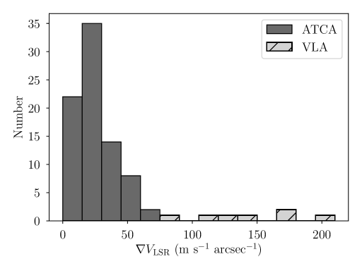
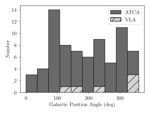
Figure 3: Histograms of the velocity gradient magnitude, $\nabla V_{\rm LSR}$, (top) and the position angle, PA, (bottom) for the ATCA and VLA H ii region samples. Only sources with RMSE less than 1.0$\,{\rm km\,s^{-1}}$ are included.

We produce composite mid-infrared/radio images for each source to help interpret the kinematic structure. We combine data from the Wide-Field Infrared Survey Explorer (WISE) with RRL and continuum data from either the ATCA or VLA. Examples are shown in Figures 4 and 5 for the ATCA H ii region G297.651$-$00.973 and the VLA H ii region G035.126$-$0.755, respectively. The color image corresponds to the WISE mid-infrared emission. H ii regions, detected in 22µm (red) emission from heated dust grains, are often surrounded by a photodissociation region, visible in 12µm (green) emission from polycyclic aromatic hydrocarbon (PAH) molecules. Overlaid on the WISE images are black contours from the free-free radio continuum that shows the extent of the H ii region. The $\langle{\rm Hn}\alpha\rangle$ RRL Gaussian fit center velocity $V_{\rm LSR}$ is represented with color contours and indicates the direction of the velocity gradient.

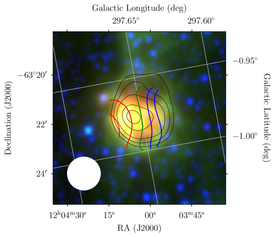
Figure 4: WISE mid-infrared image of G297.651$-$00.973. The photodissociation region (PDR) is visible at 12µm (green) from PAH emission and surrounds the H ii region detected at 22µm (red) from heated dust grains within the ionized gas. The 3.4µm (blue) emission is from low-mass stars. The ATCA free-free radio continuum emission is overlaid on the mid-infrared image as black contours at 5%, 10%, 20%, 50%, and 80% of the peak continuum brightness. The $\langle{\rm Hn}\alpha\rangle$ RRL $V_{\rm LSR}$ velocity gradient structure is shown by the colored contours. The green contour corresponds to the Gaussian center $V_{\rm LSR}$ fitted to the peak spectrum. The redshifted and blueshifted contours are spaced equally between the fitted peak Gaussian $V_{\rm LSR}$ and the maximum redshift/blueshift. The HPBW size is shown by the white circle in the bottom left-hand corner of the image.

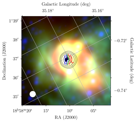
Figure 5: WISE mid-infrared image of G035.126$-$0.755. See Figure 4 for details except the radio data are from the VLA.

Some sources, such as G297.651$-$00.973 (Figure 4), show a bipolar morphology in the infrared emission. If the kinematics detected by the RRL emission were due to ionized gas motions within the bipolar outflow, we would expect the velocity gradient to be aligned with the bipolar outflow axis. For G297.651$-$00.973, the velocity gradient is perpendicular to the outflow direction, however, consistent with ionized gas rotating around the bipolar outflow; that is, the axis of rotation is along the direction of the bipolar outflow.

Another common infrared morphology is bubble-like structures. For G035.126$-$0.755 (Figure 5), we see a complex bubble morphology surrounding the radio continuum emission. We do not have the spatial resolution to infer any connection between the RRL velocity gradient and the bubble structure, but bubble infrared morphologies are common toward H ii regions (e.g., Anderson et al., 2011).

Since bulk motions can modify the line width we also inspect the morphology of the $\Delta{V}$ images. For a static nebula we expect the line width to be uniform, but we detect structure in $\Delta{V}$ images in about half of our nebulae. For example, in both G297.651$-$00.973 and G035.126$-$0.755 the line widths are higher near the center of the H ii region; that is, centrally peaked. The combination of a velocity gradient with a centrally peaked line width was also detected in the H ii region K3-50A (Balser et al., 2001). We detect centrally peaked line widths in about 15% of the sources in Tables 2 and 3. About 15% of nebulae have higher line widths toward one side of the H ii region boundary, or edge peaked. We also see a gradient in $\Delta{V}$ across nebulae in about 20% of the sources in our sample. The RRL line width morphology of the remaining sources is roughly split between uniform and complex.

4 H ii Region Simulations

To better interpret these results, we develop H ii region numerical simulations that include a dynamical model to explain the observed kinematics. Assuming an optically thin RRL in Local Thermodynamical Equilibrium (LTE), what type of dynamical model could produce RRL velocity gradients? The thermal gradient at the boundary of a spherical, homogeneous H ii region would produce a spherically symmetric expanding nebula (e.g., Spitzer, 1978; Dyson & Williams, 1997). Radiation and winds from OB-type stars could also cause expansion in young, compact H ii regions (e.g., Oey, 1996; Lopez et al., 2014; Rugel et al., 2019; McLeod et al., 2019). But a spherically symmetric expanding nebula would produce double-peaked RRL profiles toward the center of the nebula, or, if the nebula were unresolved, a square-wave profile (e.g., Balser et al., 1997). We do not detect any such profiles in the ATCA or VLA RRL data cubes, but we do see bipolar outflow morphologies in some of the mid-infrared images.

Here, we explore bipolar outflows and solid body rotation, although there may be other H ii region dynamics that can produce velocity gradients. Moreover, complex velocity structures with small spatial scales could produce velocity gradients when convolved with the telescope’s larger beam. An ionized bipolar outflow could produce a RRL velocity gradient with the velocity gradient direction aligned with the outflow axis. This depends on the relative orientation of the bipolar outflow axis with respect to the observer. A rotating spherical nebula could also produce a RRL velocity gradient where the velocity gradient direction would be normal to the rotation axis.

We assume a homogeneous, isothermal, spherical nebula and perform the radiative transfer of RRL and continuum emission to produce a model brightness temperature distribution on the sky. The spectral noise is modeled as random (Gaussian) noise with a specified RMS. We then generate synthetic RRL spectra by convolving the brightness temperature with a telescope beam. The details are given in Appendix B. These simulations produce a RRL position-position-velocity data cube. We analyze these synthetic RRL data cubes using the same procedures as for our ATCA and VLA data discussed in Section 3. We fit a single Gaussian component within each spaxel of the data cube and generate images of the center velocity, $V_{\rm LSR}$, and FWHM line width, $\Delta V$.

To investigate the effects of either bipolar outflows or solid body rotational motions, we run a series of simulations exploring a range of H ii region kinematic model parameters (see Table 4). The outflow and rotation speeds are somewhat arbitrary. Nevertheless, hydrodynamic simulations produce outflow speeds (Bodenheimer et al., 1979) and rotational speeds (Jeffreson et al., 2020) within the range of values explored in Table 4. We only consider nebulae with a diameter of 2$\,{\rm pc}$ at a distance of either 2$\,{\rm kpc}$ or 5$\,{\rm kpc}$, producing angular H ii region sizes of 206″ or 83″, respectively. Since our synthetic telescope HPBW is 90″, this corresponds to a slightly resolved or unresolved source, similar to the conditions for many of the sources in our H ii region sample.

Table 4: H ii Region Kinematic Model Parameter Ranges

Parameter	Range	Comment
$V_{\rm o}$	20–120$\,{\rm km\,s^{-1}}$	Outflow speed.
$\Theta_{\rm o}$	15–85$\,{}^{\circ}$	Outflow opening angle.
$V_{\rm eq}$	5–100$\,{\rm km\,s^{-1}}$	Rotation equatorial speed.
$\Phi_{\rm los}$	0–90$\,{}^{\circ}$	Outflow/Rotation axis relative to the line-of-sight.
$\Phi_{\rm sky}$	0–90$\,{}^{\circ}$	Position angle of the Outflow/Rotation axis on the sky.

The main results are illustrated in Figures 6 and 7 for the bipolar outflow and solid body rotation models, respectively. For each dynamical model we show the results of a simulation where the H ii region is resolved (left panels) and a simulation where the H ii region is slightly unresolved (right panels); that is, the nebular angular size is less than the HPBW. Velocity gradients are detected for both the bipolar outflow and solid body rotation model simulations. When the nebula is unresolved the synthetic $V_{\rm LSR}$ images for the bipolar outflow and solid body rotation models are very similar. The source emission is larger than the synthetic HPBW since we are detecting emission at the edge of the beam. The velocity gradient magnitude increases with better spatial resolution.

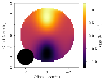
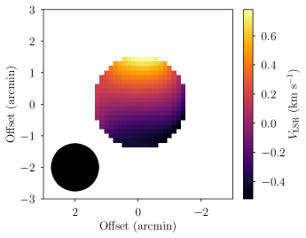
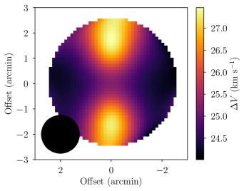
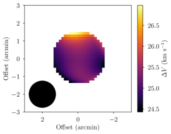
Figure 6: Bipolar outflow simulation results. The center velocity, $V_{\rm LSR}$, (top) and FWHM line width, $\Delta{V}$, (bottom) images are shown for two simulations with identical model nebulae at different distances. The resolved model nebula at a distance of 2$\,{\rm kpc}$ has an angular size of 206″ (left), whereas the unresolved model nebula at a distance of 5$\,{\rm kpc}$ has an angular size of 83″ (right). The model telescope HPBW of 90″ is shown in the bottom left-hand corner of the image. The bipolar outflow model assumes an outflow velocity $V_{\rm o}=40$$\,{\rm km\,s^{-1}}$ with opening angle of $\Theta_{\rm o}=45$$\,{}^{\circ}$. The bipolar outflow axis is tilted 45$\,{}^{\circ}$ toward the observer, $\Phi_{\rm los}=45$$\,{}^{\circ}$, and oriented north on the sky, $\Phi_{\rm sky}=0$$\,{}^{\circ}$.

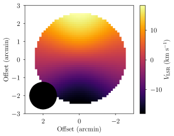
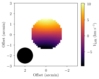
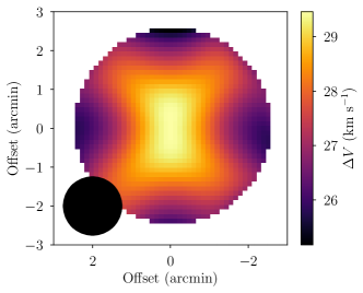
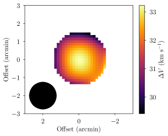
Figure 7: Solid body rotation simulation results. The center velocity, $V_{\rm LSR}$, (top) and FWHM line width, $\Delta{V}$, (bottom) images are shown for two simulations with identical model nebula at different distances. The resolved model nebulae at a distance of 2$\,{\rm kpc}$ has an angular size of 206″ (left), whereas the unresolved model nebula at a distance of 5$\,{\rm kpc}$ has an angular size of 83″ (right). The model telescope HPBW of 90″ is shown in the bottom left-hand corner of the image. The solid body rotation model assumes an equatorial speed of $V_{\rm eq}=45$$\,{\rm km\,s^{-1}}$. The rotation axis is perpendicular to the observer, $\Phi_{\rm los}=0$$\,{}^{\circ}$, and oriented East on the sky, $\Phi_{\rm sky}=90$$\,{}^{\circ}$.

There are several notable differences between the two dynamical models. When the nebula is resolved the bipolar morphology can be seen in both the $V_{\rm LSR}$ and $\Delta V$ images, given sufficient sensitivity. The solid body rotation models have a centrally peaked line width because along the center direction there is a high gradient in velocity which is blended by the beam into a broad line width.

The solid body rotation models can produce larger velocity gradients than the bipolar outflow models. This is because there are two main factors that limit the velocity gradient magnitude in the bipolar outflow models.

1. Projection Effect. There is always a significant projection effect of the outflow axis with respect to the line-of-sight. Velocity gradients are not visible if the outflow axis is pointed toward the observer ($\Phi_{\rm los}=90$$\,{}^{\circ}$) due to symmetry, or pointed normal to the line-of-sight ($\Phi_{\rm los}=0$$\,{}^{\circ}$) since there is no radial velocity component. The optimal orientation to detect a velocity gradient is when $\Phi_{\rm los}=45$$\,{}^{\circ}$, where the outflow is observed in projection. In contrast, there are no projection effects for the solid body rotation model when the rotation axis is normal to the line-of-sight ($\Phi_{\rm los}=0$$\,{}^{\circ}$). The velocity gradient does decrease as $\Phi_{\rm los}$ increases for the solid body rotation model, but there are orientations with small (or zero) projection effects.

2. Filling Factor Effect. Since the bipolar outflow model does not fill the area of the nebula as projected onto the sky, the motions of the bipolar outflow are diluted; that is, there is a filling factor that is less than one. Increasing the bipolar outflow opening angle mitigates this effect to some degree, but the magnitude of the measured velocity gradient is constrained by the RRL width. Most of the nebular emission resides at the systemic RRL velocity, so as the outflow speed is increased the emission arsing from the bipolar outflow region moves to the wings of the main Gaussian profile. This is not true for the solid body rotation models since all of the gas is rotating.

The simulations explain some of the results from our ATCA and VLA observations that are discussed in Section 3. We detect velocity gradients even when the source is not resolved because our RRL data have enough sensitivity to detect emission at the edge of the beam. We observe two sources with both the ATCA and VLA: G013.880+00.285 and G351.246+00.673 (see Tables 2–3). The velocity gradient magnitude increases with better spatial resolution, consistent with the simulations. A caveat is that the ATCA and VLA sample different spatial scales and therefore different zones of the nebula. We detect centrally peaked RRL widths in about 15% of the sources in our sample, consistent with the solid body rotation model.

Overall, the simulations favor the solid body rotation model over the bipolar outflow model for several reasons. First, we observe velocity gradients significantly larger than expected for the bipolar outflow model. The simulations are restricted to model nebulae that are either slightly resolved or unresolved, similar to our ATCA H ii region sample in Table 2 where the angular sizes are similar to the HPBW. (If the source size were significantly smaller than the HPBW, we would not be able to detect any velocity structure.) The maximum velocity gradient produced by our bipolar outflow model simulations is about 40$\,{\rm m\,s^{-1}\,arcsec^{-1}}$, yet we detect velocity gradients significantly higher in the ATCA H ii region sample. The parameters for the bipolar outflow model with the maximum velocity gradient are: $V_{\rm o}=30$$\,{\rm km\,s^{-1}}$, $\Theta_{\rm o}=85$$\,{}^{\circ}$, and $\Phi_{\rm los}=45$$\,{}^{\circ}$. For this model the nebula is unresolved. Increasing the outflow velocity beyond $V_{\rm o}=30$$\,{\rm km\,s^{-1}}$ reduces the velocity gradient because of the filling factor effect discussed above. In contrast, there is no such limitation for the solid body rotation model because all of the gas is rotating. For solid body rotation with $V_{\rm eq}=15$$\,{\rm km\,s^{-1}}$ and $\Phi_{\rm los}=0$$\,{}^{\circ}$, the simulation produces a velocity gradient of $\nabla V_{\rm LSR}=83$$\,{\rm m\,s^{-1}\,arcsec^{-1}}$ for an unresolved nebula. Increasing the equatorial rotation speed increases the velocity gradient. Second, the bipolar outflow model simulations predict that we should see a bipolar morphology when the nebula is resolved, but we do not observe any bipolar structure in the $V_{\rm LSR}$ images. Lastly, we detect a centrally peaked RRL width in about 15% of our sources, consistent with the solid body rotation model.

The model H ii region simulations discussed here are limited. They only include simple dynamical models for bipolar outflows and rotational motions. Moreover, we have not explored the full model parameter phase space. More sophisticated Monte Carlo simulations could make predictions about the expected distribution of velocity gradient magnitudes, but this is beyond the scope of this paper. Nevertheless, the solid body rotation models are better able to reproduce the velocity gradient properties determined from our H ii regions RRL observations.

5 Discussion

Rotation is a common property of most objects in the Milky Way (Belloche, 2013). On the largest scales there is differential rotation in the Galactic disk. Simulations indicate that the rotational properties of H i clouds and GMCs are correlated with the time scale for Galactic shearing and the gravitational free-fall time (Jeffreson et al., 2020). The specific angular momentum of the stars and planets that form within GMCs is about six orders of magnitude less than the dense cores in GMCs (Belloche, 2013). Since angular momentum is conserved there must be a transfer of angular moment during star formation, but the possible candidates (e.g., fragmentation, magnetic braking, etc.) cannot explain the difference; hence the “Angular Momentum Problem” in star formation (Spitzer, 1978; Bodenheimer, 1995; Mathieu, 2004).

Where do the dense cores in GMCs obtain their angular momentum? Results from Herschel indicate that most molecular cores form in filaments with a typical width of 0.1$\,{\rm pc}$ (André et al., 2010, 2014; Koch & Rosolowsky, 2015). These molecular filaments tend to have sizes between the GMCs and the molecular cores. Hsieh et al. (2021) performed observations of N₂D⁺ in Orion B and detect a velocity gradient along the molecular filament’s minor axis. The authors argue that the velocity gradient is due to rotation of the filament and that the derived angular momentum profile, how the angular momentum varies with distance from the center of the filament, is consistent with ambient turbulence as the source of the filament’s rotation (see Misugi et al., 2019). Tracing the angular momentum through the stages of gravitational collapse that lead to high mass star formation is a fundamental problem that calls for further simulations and observations with various ISM tracers.

Dalgleish et al. (2018) use the simulations of Peters et al. (2010a) to develop a cartoon picture of how H ii regions kinematically evolve. Peters et al. (2010a) use the FLASH code to develop three-dimensional simulations of a rotating, collapsing molecular cloud and include heating from both ionizing and non-ionizing sources (also see Peters et al., 2010c, b). The simulation begins with a molecular cloud which has a net angular momentum. Stars form in the denser regions and follow the rotation of the cloud. The angular momentum of the H ii region is inherited from the parent cloud only indirectly, via these massive ionizing stars, whose motions within the expanding H ii region complicate the dynamics of the ionized gas. Nevertheless, Dalgleish et al. (2018) predict that most H ii regions should contain the kinematic signature of rotation—velocity gradients.

We detect velocity gradients between $\nabla V_{\rm LSR}=5-200$$\,{\rm m\,s^{-1}\,arcsec^{-1}}$ in about 49% of the sources in our H ii region sample. Moreover, the RRL widths are centrally peaked in about 15% of the sources with velocity gradients. Simple models of solid body rotation can produce velocity gradients with similar magnitudes as observed and have centrally peaked line widths. These results are all consistent with the hypothesis that most H ii regions have inherited some of the angular momentum from their rotating parent molecular clouds.

We cannot, however, rule out other dynamical models. We have shown that nebula models of bipolar outflow also predict velocity gradients. Moreover, bipolar outflow structure is observed in infrared emission toward some sources in our sample with detected velocity gradients. If the velocity gradient were due to the bipolar outflow motions then the velocity gradient should be along the direction of the bipolar outflow axis. Another possibility is that the velocity gradient is primarily due to rotation from a disk of material and the bipolar outflow is aligned with the rotation axis (e.g., G297.651$-$00.973 in Figure 4). We only detect an infrared bipolar morphology in about 10 sources from our sample and there is no consistent alignment between the bipolar morphology axis and the RRL velocity gradient direction. There are examples in the literature where there is evidence for both rotation and a bipolar outflow in the ionized gas: NGC 6334A (De Pree et al., 1995; Balser et al., 2001), K3-50A (De Pree et al., 1994; Balser et al., 2001), W49A (Mufson & Liszt, 1977; Welch et al., 1987), and G316.81–0.06 (Dalgleish et al., 2018).

To distinguish between these two dynamical models requires better spatial resolution. In some cases both rotation and outflow may be present but they may occur on different spatial scales. The H ii region NGC 6334A is a good example where the bipolar outflow extends beyond the core region and the kinematics can be separated with position-velocity maps (Balser et al., 2001). Regardless, the simple bipolar outflow model developed here cannot explain many of the velocity gradients in our sample because these models are unable to produce the large velocity gradients or the centrally peaked line widths. More complex models could overcome some of these limitations. For example, a bipolar outflow H ii region where the density is significantly enhanced in the outflow region.

Dalgleish et al. (2018) speculate that if Galactic rotation provides the initial angular momentum of molecular clouds then there should be a connection between the orientation of the angular momentum axis of the molecular cloud and the Galactic plane (also see Garay et al., 1986). Figure 3 plots the velocity gradient position angle distribution with respect to Galactic Plane. Since the position angle distribution is approximately random, there is no evidence that the initial angular momentum of the molecular clouds from which the H ii regions formed is set by Galactic rotation.

The ATCA and VLA RRL surveys provide a nice sample to explore H ii region kinematics and provide constraints on how angular momentum governs star formation. More sensitive, higher spatial resolution images of the H ii regions in our sample are necessary to disentangle the effects of feedback mechanisms such as outflows from properties like rotation.

6 Summary

Over the last decade we have doubled the number of known H ii regions in the Milky Way by detecting RRL emission at 4–10$\,{\rm GHz}$ toward candidate H ii regions that were identified by their mid-infrared and radio continuum morphology. This was achieved by the improved spectral sensitivity of the GBT in the northern sky (HRDS) and the ATCA in the southern sky (SHRDS). A total of $\sim 1400$ H ii regions have been discovered and the current census now includes all nebulae ionized by a single O9 V-type star at a distance of $\sim 10$$\,{\rm kpc}$. We also used the VLA to observe a subset of the HRDS to derive accurate electron temperatures which are a proxy for metallicity.

Here we use ATCA and VLA RRL data to create a sample of 425 independent observations of 374 H ii regions that are suitable for kinematic analysis. We select sources that are relatively well isolated and have a single RRL profile with a SNR greater than 10. We perform Gaussian fits of the RRL position-position-velocity data cubes and discover velocity gradients in about 40% of the nebulae. Velocity gradient magnitudes range between about 5 and 200$\,{\rm m\,s^{-1}\,arcsec^{-1}}$. We also detect centrally peaked RRL widths in about 15% of the sources. The velocity gradient position angles appear to be random on the sky with no favored orientation with respect to the Galactic Plane.

To better interpret these results we develop simulations to produce synthetic RRL observations toward model nebulae. Assuming a homogeneous, isothermal spherical nebula we perform the radiative transfer of RRL and continuum emission on the sky and convolve the resulting brightness distribution with a telescope antenna pattern to produce synthetic RRL data cubes. We consider two dynamical models: bipolar outflow and solid body rotation. Both dynamical models produce velocity gradients that have similar characteristics for unresolved nebulae. The solid body rotation model produces both the full range of velocity gradient magnitudes and centrally peaked line widths. In contrast, the bipolar outflow model cannot produce the observed velocity gradients $>40$$\,{\rm m\,s^{-1}\,arcsec^{-1}}$ nor the centrally peaked line widths for the simulations discussed here. We therefore favor the solid body rotation model, but we cannot rule out that bipolar outflows are causing the velocity gradients in some of our sources. There are several examples in our sample and in the literature of H ii regions that show evidence for both rotation and outflow. Observations with higher spatial resolution are required to distinguish between these models for many of our sources.

Appendix A Fitting Models to Correlated Image Data

A model $M$ predicts $\bm{y}=(y_{0},y_{1},\dots,y_{N})$ given independent data $\bm{x}=(x_{0},x_{y},\dots,x_{N})$ and model parameters $\bm{\theta}$. The generalized Gaussian log-likelihood function is

$$\ln L=-0.5N\ln 2\pi-0.5\ln|\bm{\Sigma}|-0.5\left(\bm{y}-M(\bm{x},\bm{\theta})\right)^{T}\bm{\Sigma}^{-1}\left(\bm{y}-M(\bm{x},\bm{\theta})\right),$$ (A1)

where $\bm{\Sigma}$ is the covariance matrix.

The generalized Gaussian likelihood function is simplified under the assumption of independent and identically distributed (i.d.d.) observed data. In this scenario, the covariance matrix has zeros every except along the diagonal, where $\Sigma_{i,i}=\sigma^{2}_{y,i}$ and $\bm{\sigma^{2}_{y}}=(\sigma^{2}_{y,0},\sigma^{2}_{y,1},\dots,\sigma^{2}_{y,N})$ are the observed data variances. The determinant of this covariance matrix is $|\bm{\Sigma}|=\sum^{N}\sigma^{2}_{y,i}$ and so the log-likelihood function is

$$\ln L=-0.5N\ln 2\pi-0.5\sum^{N}\sigma^{2}_{y,i}-0.5\sum^{N}\frac{\left(y_{i}-M(x_{i},\bm{\theta})\right)^{2}}{\sigma^{2}_{y,i}}.$$ (A2)

Maximizing this log-likelihood function is equivalent to reducing the last term, which is the sum of the squared residuals weighted by the observed data variances.

In general, the covariance matrix is populated with elements $\Sigma_{i,j}=\rho_{i,j}\sigma_{i}\sigma_{j}$ where $\sigma_{i}$ and $\sigma_{j}$ are the standard deviations of the observed data $y_{i}$ and $y_{j}$, respectively, and $\rho_{i,j}$ is the correlation coefficient between $y_{i}$ and $y_{j}$. In an image with a Gaussian resolution element, the correlation coefficient between pixel $i$ and pixel $j$ is

$$\rho_{i,j}=\exp\left[-A\Delta x^{2}-2B\Delta x\Delta y-C\Delta y^{2}\right]\,,$$ (A3)

where

$$A =\frac{\cos^{2}\phi}{2\theta_{\rm maj}^{2}}+\frac{\sin^{2}\phi}{2\theta_{\rm min}^{2}}\,,$$

$$B =-\frac{\sin(2\phi)}{4\theta_{\rm maj}^{2}}+\frac{\sin(2\phi)}{4\theta_{\rm min}^{2}}\,,$$

$$C =\frac{\sin^{2}\phi}{2\theta_{\rm maj}^{2}}+\frac{\cos^{2}\phi}{2\theta_{\rm min}^{2}}\,,$$

$\Delta x$ and $\Delta y$ are the separations between the $i$th and $j$th pixels in the east-west and north-south directions, respectively, and $\theta_{\rm maj}$, $\theta_{\rm min}$, and $\phi$ are the synthesized beam major axis, minor axis, and north-through-east position angle, respectively (see Wenger et al., 2019a).

The generalized covariance matrix is typically ill-conditioned; the determinant and inverted matrix are susceptible to numerical precision loss. Therefore, we truncate the correlation coefficient at $\rho=0.5$, which is equivalent to the expected correlation between two points separated by half of the half-power beam-width.

For a polynomial model, $M(\bm{x},\bm{\theta})=\bm{D}\bm{\theta}$ where $\bm{D}$ is the design matrix with elements $D_{i,j}=x_{i}^{j}$. With this notation, the log-likelihood function is

$$\ln L=-0.5(\bm{y}-\bm{D}\bm{\theta})^{T}\bm{\Sigma}^{-1}(\bm{y}-\bm{D}\bm{\theta})+const.$$ (A4)

Maximizing this function is identical to generalized least squares. Equating the derivative of the log-likelihood with respect to $\bm{\theta}$ to zero, we solve for the parameters $\hat{\bm{\theta}}$ that maximize the log-likelihood:

$$\frac{\partial\,({\rm ln}\,L)}{\partial\bm{\theta}}=0 =-\bm{D}^{T}\bm{\Sigma}^{-1}(\bm{y}-\bm{D}\hat{\bm{\theta}})$$

$$=-\bm{D}^{T}\bm{\Sigma}^{-1}\bm{y}+\bm{D}^{T}\bm{\Sigma}^{-1}\bm{D}\hat{\bm{\theta}}$$

$$\hat{\bm{\theta}} =(\bm{D}^{T}\bm{\Sigma}^{-1}\bm{D})^{-1}\bm{D}^{T}\bm{\Sigma}^{-1}\bm{y}.$$ (A5)

A.1 Velocity Gradient Fit to a Plane Model

To characterize the observed velocity gradients we fit the $V_{\rm LSR}$ image to a plane defined by

$$z=c_{0}+c_{1}\,x+c_{2}\,y,$$ (A6)

where ($x,y$) are the pixel coordinates on the sky, $z$ is the LSR velocity, and ($c_{0},c_{1},c_{2}$) are constants. The magnitude of the velocity gradient is

$$\nabla V_{\rm LSR}=\sqrt{c_{1}^{2}+c_{2}^{2}},$$ (A7)

and the position angle,

$${\rm PA}={\rm arctan}(c_{2}/c_{1}).$$ (A8)

The offset velocity is given by $c_{0}$. We use Maximum Likelihood Estimation as described in §A to determine the best fit taking into account the errors in $V_{\rm LSR}$ and that nearby pixels are correlated; that is, there are several pixels across the synthesized HPBW. The position angle is defined to be zero along the north direction, increasing eastward in Equatorial coordinates.

Appendix B H ii Region Model

To explore the effects of different dynamical models on the observed RRL kinematics, we develop a numerical code in Python to simulation a RRL and continuum emission observation (Ref, TBD). We assume a homogeneous, isothermal, spherical nebula consisting of fully ionized hydrogen with electron density $n_{\rm e}$ and electron temperature $T_{\rm e}$. In practice the electron density and temperature vary within an H ii region (Roelfsema et al., 1992; Balser & Bania, 2018), but here we keep the models simple. We include RRL and free-free continuum emission assuming local thermodynamic equilibrium (LTE). Following Condon & Ransom (2016), the RRL absorption coefficient as a function of frequency, $\nu$, is given by

$$\kappa_{\rm L}(\nu)=\frac{c^{2}}{8\pi\nu_{\rm o}^{2}}\frac{g_{\rm u}}{g_{\rm l}}n_{\rm l}A_{\rm ul}\left[1-{\rm exp}\left(-\frac{h\nu_{\rm o}}{kT_{\rm e}}\right)\right]\phi(\nu),$$ (B1)

where $c$ is the speed of light, $h$ is Planck’s constant, $k$ is Boltzmann’s constant, $\nu_{\rm o}$ is the frequency of the RRL transition, $A_{\rm ul}$ is the spontaneous emission rate from the upper to the lower state, and $n_{\rm l}$ is the number density in the lower state. The spontaneous emission rate can be approximated as

$$A_{\rm n+1,n}=\left(\frac{64\pi^{6}m_{\rm e}e^{10}}{3c^{3}h^{6}}\right)\frac{1}{n^{5}},$$ (B2)

where $m_{\rm e}$ is the electron mass and n is the principal quantum number (Condon & Ransom, 2016). The statistical weights for hydrogen are given by $g_{\rm n}=2{\rm n}^{2}$. We assume a Gaussian line profile, $\phi(\nu)$, that is broadened by thermal motions of the gas characterized by the FWHM line width, $\Delta V_{\rm t}$. A non-thermal component, $\Delta V_{\rm nt}$, is included to account for any turbulent motions and is added in quadrature to the thermal width to derive the total line width.

H ii regions also produce continuous, free-free thermal bremsstrahlung emission. From Condon & Ransom (2016), the free-free absorption coefficient is given by

$$\kappa_{\rm C}(\nu)=\frac{1}{\nu^{2}T_{\rm e}^{3/2}}\left[\frac{Z^{2}e^{6}}{c}n_{\rm e}n_{\rm i}\frac{1}{\sqrt{2\pi(m_{\rm e}k)^{3}}}\right]\frac{\pi^{2}}{4}ln\left(\frac{b_{\rm max}}{b_{\rm min}}\right),$$ (B3)

where $Z$ is the effective nuclear charge number, $e$ is the charge, $n_{\rm i}$ is the ion number density, and $b_{\rm min}$ and $b_{\rm min}$ are the minimum and maximum impact parameters, respectively. Following Condon & Ransom (2016), we estimate the impact parameter ratio by

$$\frac{b_{\rm max}}{b_{\rm min}}=\left(\frac{3kT_{\rm e}}{m_{\rm e}}\right)^{3/2}\frac{m_{\rm e}}{2\pi Ze^{2}\nu}.$$ (B4)

Assuming the Rayleigh-Jeans limit, $h\nu\ll kT_{\rm e}$, the brightness temperature is given by

$$T_{\rm B}=T_{\rm e}(1-{\rm e}^{-\tau}),$$ (B5)

where $\tau$ is the optical depth, $\tau=\int\kappa\,d\ell$, and $d\ell$ is the path length through the nebula. We perform the radiative transfer through the nebula to determine the brightness distribution on the sky ($\rm\,Jy\,arcsec^{-2}$) as a function of frequency. The spectral noise is modeled as random (Gaussian) noise with a specified RMS. Synthetic spectra are produced by convolving the brightness distribution on the sky with a telescope beam to determine the observed brightness distribution ($\rm\,Jy\,beam^{-1}$). We assume a Gaussian telescope beam shape with a specified HPBW. The nebular angular size is given by $\theta_{\rm s}=D/R_{\rm Sun}$, where $D$ is the diameter of the spherical nebula and $R_{\rm Sun}$ is the distance.

The model H ii region properties are listed in Table 5 with their default values. Unless noted otherwise we use the default values for all simulations. In addition to the thermal and non-thermal motions that are constant within the nebula, we include bulk motions that are described by a dynamical model. Below we consider bipolar outflow and solid body rotation models.

Table 5: Model H ii Region Properties

Property	Symbol	Default Value	Comment
Electron density	$n_{\rm e}$	250$\,{\rm cm^{-3}}$	Homogeneous nebula.
Electron temperature	$T_{\rm e}$	8000$\,{\rm K}$	Isothermal nebula.
Non-thermal line width	$\Delta V_{\rm nt}$	15$\,{\rm km\,s^{-1}}$
Diameter	$D$	2$\,{\rm pc}$	Spherical nebula.
Distance	$R_{\rm Sun}$	5$\,{\rm kpc}$
RRL	Hn$\alpha$	H85$\alpha$	$\Delta{\rm n}=1$ correspond to $\alpha$ transitions.
RMS spectral noise	$N$	0.001$\rm\,mJy\,arcsec^{-2}$	Gaussian noise.
Telescope HPBW	$\theta_{\rm b}$	90″	Gaussian profile.
Outflow speed	$V_{\rm o}$	…	Bipolar outflow model.
Outflow opening angle	$\Theta_{\rm o}$	…	Bipolar outflow model.
Rotation equatorial speed	$V_{\rm eq}$	…	Solid body rotation model; speed at the equator.
Line-of-sight angle	$\Phi_{\rm los}$	…	Bipolar outflow and solid body rotation models.
Sky position angle	$\Phi_{\rm sky}$	…	Bipolar outflow and solid body rotation models.

B.1 Bipolar Outflow

Outflows are a common phenomena in astrophysics and may explain the observed velocity gradients. We assume that the bipolar outflow emanates radially from the center of the H ii region sphere and is defined by a constant outflow speed, $V_{\rm o}$, with opening angle, $\Theta_{\rm o}$ (see Figure 8). The outflow orientation is defined by two angles: the position angle relative to the line-of-sight, $\Phi_{\rm los}$, and the position angle on the sky, $\Phi_{\rm sky}$. The angle $\Phi_{\rm los}$ is zero normal to the observer and 90$\,{}^{\circ}$ along the line-of-sight. The angle $\Phi_{\rm sky}$ is defined to be zero when oriented north and increases to the east.

B.2 Solid Body Rotation

Rotation is a common property in astrophysics and we might expect that all H ii region complexes inherit some angular momentum, and thus rotation, from their parent molecular cloud. Here we explore solid body rotation for simplicity, but differential rotation is also possible. The magnitude of the solid body rotation is defined by the equatorial speed, $V_{\rm eq}$, and the orientation of the angular momentum vector is defined by the two position angles: $\Phi_{\rm los}$ and $\Phi_{\rm sky}$ (see Figure 8). The rotation axis is the direction of the angular momentum vector, so the angle $\Phi_{\rm los}$ is zero normal to the observer and 90$\,{}^{\circ}$ along the line-of-sight. The angle $\Phi_{\rm sky}$ is defined to be zero when oriented north and increases to the east.

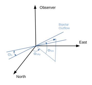
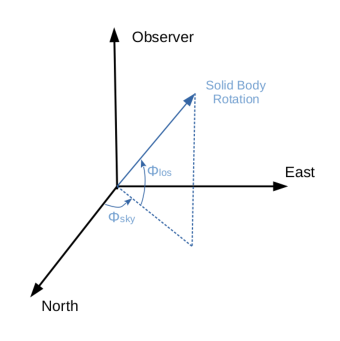
Figure 8: Geometry of the bipolar outflow (left) and solid body rotation (right) dynamical models. The observer is located along the z-axis, looking down on the x-y plane. The angle of the outflow or rotation axis relative to the line-of-sight, $\Phi_{\rm los}$, is 90$\,{}^{\circ}$ when pointing towards the observer. The position angle of the outflow or rotation axis on the sky, $\Phi_{\rm sky}$, is zero when pointing to the north. For the bipolar outflow model the opening angle of the outflow, assumed to be symmetric, is given by $\Theta_{\rm o}$.

References

- Ali et al. (2018) Ali, A., Harries, T. J., & Douglas, T. A. 2018, MNRAS, 477, 5422, doi: 10.1093/mnras/sty1001
- Anderson et al. (2015) Anderson, L. D., Armentrout, W. P., Johnstone, B. M., et al. 2015, ApJS, 221, 26, doi: 10.1088/0067-0049/221/2/26
- Anderson et al. (2018) Anderson, L. D., Armentrout, W. P., Luisi, M., et al. 2018, ApJS, 234, 33, doi: 10.3847/1538-4365/aa956a
- Anderson et al. (2011) Anderson, L. D., Bania, T. M., Balser, D. S., & Rood, R. T. 2011, ApJS, 194, 32, doi: 10.1088/0067-0049/194/2/32
- André et al. (2014) André, P., Di Francesco, J., Ward-Thompson, D., et al. 2014, in Protostars and Planets VI, ed. H. Beuther, R. S. Klessen, C. P. Dullemond, & T. Henning, 27, doi: 10.2458/azu_uapress_9780816531240-ch002
- André et al. (2010) André, P., Men’shchikov, A., Bontemps, S., et al. 2010, A&A, 518, L102, doi: 10.1051/0004-6361/201014666
- Arquilla & Goldsmith (1985) Arquilla, R., & Goldsmith, P. F. 1985, ApJ, 297, 436, doi: 10.1086/163542
- Balser (2006) Balser, D. S. 2006, AJ, 132, 2326, doi: 10.1086/508515
- Balser & Bania (2018) Balser, D. S., & Bania, T. M. 2018, AJ, 156, 280, doi: 10.3847/1538-3881/aaeb2b
- Balser et al. (1997) Balser, D. S., Bania, T. M., Rood, R. T., & Wilson, T. L. 1997, ApJ, 483, 320, doi: 10.1086/304248
- Balser et al. (2001) Balser, D. S., Goss, W. M., & De Pree, C. G. 2001, AJ, 121, 371, doi: 10.1086/318028
- Bania et al. (2012) Bania, T. M., Anderson, L. D., & Balser, D. S. 2012, ApJ, 759, 96, doi: 10.1088/0004-637X/759/2/96
- Bania et al. (2010) Bania, T. M., Anderson, L. D., Balser, D. S., & Rood, R. T. 2010, ApJ, 718, L106, doi: 10.1088/2041-8205/718/2/L106
- Beckman & Relaño (2004) Beckman, J. E., & Relaño, M. 2004, Ap&SS, 292, 111, doi: 10.1023/B:ASTR.0000045006.88476.b6
- Belloche (2013) Belloche, A. 2013, in EAS Publications Series, Vol. 62, EAS Publications Series, ed. P. Hennebelle & C. Charbonnel, 25–66, doi: 10.1051/eas/1362002
- Bodenheimer (1995) Bodenheimer, P. 1995, ARA&A, 33, 199, doi: 10.1146/annurev.aa.33.090195.001215
- Bodenheimer et al. (1979) Bodenheimer, P., Tenorio-Tagle, G., & Yorke, H. W. 1979, ApJ, 233, 85, doi: 10.1086/157368
- Bordalo et al. (2009) Bordalo, V., Plana, H., & Telles, E. 2009, ApJ, 696, 1668, doi: 10.1088/0004-637X/696/2/1668
- Bresolin et al. (2020) Bresolin, F., Rizzi, L., Ho, I. T., et al. 2020, MNRAS, 495, 4347, doi: 10.1093/mnras/staa1472
- Brown et al. (2017) Brown, C., Jordan, C., Dickey, J. M., et al. 2017, AJ, 154, 23, doi: 10.3847/1538-3881/aa71a7
- Caselli et al. (2002) Caselli, P., Benson, P. J., Myers, P. C., & Tafalla, M. 2002, ApJ, 572, 238, doi: 10.1086/340195
- Chen et al. (2007) Chen, X., Launhardt, R., & Henning, T. 2007, ApJ, 669, 1058, doi: 10.1086/521868
- Churchwell (2002) Churchwell, E. 2002, ARA&A, 40, 27, doi: 10.1146/annurev.astro.40.060401.093845
- Condon & Ransom (2016) Condon, J. J., & Ransom, S. M. 2016, Essential Radio Astronomy
- Dalgleish et al. (2018) Dalgleish, H. S., Longmore, S. N., Peters, T., et al. 2018, MNRAS, 478, 3530, doi: 10.1093/mnras/sty1109
- De Pree et al. (1994) De Pree, C. G., Goss, W. M., Palmer, P., & Rubin, R. H. 1994, ApJ, 428, 670, doi: 10.1086/174277
- De Pree et al. (1995) De Pree, C. G., Rodriguez, L. F., Dickel, H. R., & Goss, W. M. 1995, ApJ, 447, 220, doi: 10.1086/175868
- Dyson & Williams (1997) Dyson, J. E., & Williams, D. A. 1997, The physics of the interstellar medium, doi: 10.1201/9780585368115
- Ferland (2001) Ferland, G. J. 2001, PASP, 113, 41, doi: 10.1086/317983
- Fleck & Clark (1981) Fleck, R. C., J., & Clark, F. O. 1981, ApJ, 245, 898, doi: 10.1086/158866
- Garay et al. (1986) Garay, G., Rodriguez, L. F., & van Gorkom, J. H. 1986, ApJ, 309, 553, doi: 10.1086/164624
- Goodman et al. (1993) Goodman, A. A., Benson, P. J., Fuller, G. A., & Myers, P. C. 1993, ApJ, 406, 528, doi: 10.1086/172465
- Hsieh et al. (2021) Hsieh, C.-H., Arce, H. G., Mardones, D., Kong, S., & Plunkett, A. 2021, ApJ, 908, 92, doi: 10.3847/1538-4357/abd034
- Hunter (2007) Hunter, J. D. 2007, Computing in Science Engineering, 9, 90, doi: 10.1109/MCSE.2007.55
- Imara & Blitz (2011) Imara, N., & Blitz, L. 2011, ApJ, 732, 78, doi: 10.1088/0004-637X/732/2/78
- Jaffe et al. (2005) Jaffe, D., Zhu, Q., Lacy, J., Richter, M., & Greathouse, T. 2005, in High Resolution Infrared Spectroscopy in Astronomy, 162–167, doi: 10.1007/10995082_26
- Jeffreson et al. (2020) Jeffreson, S. M. R., Kruijssen, J. M. D., Keller, B. W., Chevance, M., & Glover, S. C. O. 2020, MNRAS, doi: 10.1093/mnras/staa2127
- Kass & Raftery (1995) Kass, R. E., & Raftery, A. E. 1995, Journal of the American Statistical Association, 90, 773, doi: 10.1080/01621459.1995.10476572
- Keto & Wood (2006) Keto, E., & Wood, K. 2006, ApJ, 637, 850, doi: 10.1086/498611
- Koch & Rosolowsky (2015) Koch, E. W., & Rosolowsky, E. W. 2015, MNRAS, 452, 3435, doi: 10.1093/mnras/stv1521
- Lebouteiller et al. (2012) Lebouteiller, V., Cormier, D., Madden, S. C., et al. 2012, A&A, 548, A91, doi: 10.1051/0004-6361/201218859
- Lopez et al. (2014) Lopez, L. A., Krumholz, M. R., Bolatto, A. D., et al. 2014, ApJ, 795, 121, doi: 10.1088/0004-637X/795/2/121
- Luisi et al. (2021) Luisi, M., Anderson, L. D., Schneider, N., et al. 2021, arXiv e-prints, arXiv:2104.04568. https://arxiv.org/abs/2104.04568
- Markwardt (2009) Markwardt, C. B. 2009, in Astronomical Society of the Pacific Conference Series, Vol. 411, Astronomical Data Analysis Software and Systems XVIII, ed. D. A. Bohlender, D. Durand, & P. Dowler, 251. https://arxiv.org/abs/0902.2850
- Mathieu (2004) Mathieu, R. D. 2004, in Stellar Rotation, ed. A. Maeder & P. Eenens, Vol. 215, 113
- McLeod et al. (2019) McLeod, A. F., Dale, J. E., Evans, C. J., et al. 2019, MNRAS, 486, 5263, doi: 10.1093/mnras/sty2696
- Mermilliod & García (2001) Mermilliod, J.-C., & García, B. 2001, in The Formation of Binary Stars, ed. H. Zinnecker & R. Mathieu, Vol. 200, 191
- Misugi et al. (2019) Misugi, Y., Inutsuka, S.-i., & Arzoumanian, D. 2019, ApJ, 881, 11, doi: 10.3847/1538-4357/ab2382
- Morris et al. (1974) Morris, M., Zuckerman, B., Turner, B. E., & Palmer, P. 1974, ApJ, 192, L27, doi: 10.1086/181581
- Mouschovias (1975) Mouschovias, T. C. 1975, PhD thesis, California Univ., Berkeley.
- Mufson & Liszt (1977) Mufson, S. L., & Liszt, H. S. 1977, ApJ, 212, 664, doi: 10.1086/155089
- Nicholls et al. (2012) Nicholls, D. C., Dopita, M. A., & Sutherland, R. S. 2012, ApJ, 752, 148, doi: 10.1088/0004-637X/752/2/148
- Oey (1996) Oey, M. S. 1996, ApJ, 465, 231, doi: 10.1086/177415
- Okamoto et al. (2003) Okamoto, Y. K., Kataza, H., Yamashita, T., et al. 2003, ApJ, 584, 368, doi: 10.1086/345540
- Peters et al. (2010a) Peters, T., Banerjee, R., Klessen, R. S., et al. 2010a, ApJ, 711, 1017, doi: 10.1088/0004-637X/711/2/1017
- Peters et al. (2010b) Peters, T., Klessen, R. S., Mac Low, M.-M., & Banerjee, R. 2010b, ApJ, 725, 134, doi: 10.1088/0004-637X/725/1/134
- Peters et al. (2010c) Peters, T., Mac Low, M.-M., Banerjee, R., Klessen, R. S., & Dullemond, C. P. 2010c, ApJ, 719, 831, doi: 10.1088/0004-637X/719/1/831
- Roelfsema et al. (1992) Roelfsema, P. R., Goss, W. M., & Mallik, D. C. V. 1992, ApJ, 394, 188, doi: 10.1086/171570
- Rubin (1985) Rubin, R. H. 1985, ApJS, 57, 349, doi: 10.1086/191007
- Rugel et al. (2019) Rugel, M. R., Rahner, D., Beuther, H., et al. 2019, A&A, 622, A48, doi: 10.1051/0004-6361/201834068
- Russeil et al. (2016) Russeil, D., Tigé, J., Adami, C., et al. 2016, A&A, 587, A135, doi: 10.1051/0004-6361/201424484
- Spitzer (1978) Spitzer, L. 1978, Physical processes in the interstellar medium, doi: 10.1002/9783527617722
- Tobin et al. (2011) Tobin, J. J., Hartmann, L., Chiang, H.-F., et al. 2011, ApJ, 740, 45, doi: 10.1088/0004-637X/740/1/45
- Torres-Flores et al. (2013) Torres-Flores, S., Barbá, R., Maíz Apellániz, J., et al. 2013, A&A, 555, A60, doi: 10.1051/0004-6361/201220474
- van der Walt et al. (2011) van der Walt, S., Colbert, S. C., & Varoquaux, G. 2011, Computing in Science Engineering, 13, 22, doi: 10.1109/MCSE.2011.37
- Veilleux et al. (2005) Veilleux, S., Cecil, G., & Bland-Hawthorn, J. 2005, ARA&A, 43, 769, doi: 10.1146/annurev.astro.43.072103.150610
- Welch et al. (1987) Welch, W. J., Dreher, J. W., Jackson, J. M., Terebey, S., & Vogel, S. N. 1987, Science, 238, 1550, doi: 10.1126/science.238.4833.1550
- Wenger et al. (2019a) Wenger, T. V., Balser, D. S., Anderson, L. D., & Bania, T. M. 2019a, ApJ, 887, 114, doi: 10.3847/1538-4357/ab53d3
- Wenger et al. (2019b) Wenger, T. V., Dickey, J. M., Jordan, C. H., et al. 2019b, ApJS, 240, 24, doi: 10.3847/1538-4365/aaf8ba
- Wenger et al. (2021) Wenger, T. V., Dawson, J. R., Dickey, J. M., et al. 2021, arXiv e-prints, arXiv:2103.12199. https://arxiv.org/abs/2103.12199
- Zhu (2006) Zhu, Q. 2006, PhD thesis, The University of Texas at Austin