The impact of transverse Slavnov-Taylor identities on dynamical chiral symmetry breaking

Abstract

We extend earlier studies of transverse Ward-Fradkin-Green-Takahashi identities in QED, their usefulness to constrain the transverse fermion-boson vertex and their importance for multiplicative renormalizability, to the equivalent gauge identities in QCD. To this end, we consider transverse Slavnov-Taylor identities that constrain the transverse quark-gluon vertex and derive its eight associated scalar form factors. The complete vertex can be expressed in terms of the quark’s mass and wave-renormalization functions, the ghost-dressing function, the quark-ghost scattering amplitude and a set of eight form factors. The latter parametrize the hitherto unknown nonlocal tensor structure in the transverse Slavnov-Taylor identity which arises from the Fourier transform of a four-point function involving a Wilson line in coordinate space. We determine the functional form of these eight form factors with the constraints provided by the Bashir-Bermudez vertex and study the effects of this novel vertex on the quark in the Dyson-Schwinger equation using lattice QCD input for the gluon and ghost propagators. We observe significant dynamical chiral symmetry breaking and a mass gap that leads to a constituent mass of the order of 500 MeV for the light quarks. The flavor dependence of the mass and wave-renormalization functions as well as their analytic behavior on the complex momentum plane is studied and as an application we calculate the quark condensate and the pion’s weak decay constant in the chiral limit. Both are in very good agreement with their reference values.

1 Introduction

Whilst the Brout-Englert-Higgs (BEH) mechanism has been established as the essential explicit source of elementary particles’ masses, the same cannot be said of Nature’s composite building blocks, namely the atoms and their nuclei. Even the lightest Nambu-Goldstone mode of Quantum Chromodynamics (QCD), the pion, is more than an order of magnitude heavier than the sum of the current masses of its constituents provided by the BEH mechanism. QCD is not a conformal theory and this mass relation is only sensible at a certain energy scale. Commonly, the light quark’s current masses are quoted at 2 GeV in the $\overline{\rm MS}$ scheme Aoki:2019cca , at which the sum of two $u$ and one $d$ current-quark current masses amounts to merely 1% of the proton mass.

The overwhelming contribution to the light hadron’s masses does not stem from the aforementioned mechanism and a recent lattice-QCD simulation Yang:2018nqn concludes that the kinetic quark energy and the gluon field are together responsible for 68% of the proton mass, whereas the trace anomaly contributes 23%. Thus, only 9% of the proton’s mass is due to the scalar condensate, which exhibits the major current-quark mass dependence. This recent analysis of the proton’s “mass budget” has come to strengthen long-standing observations made by groups who apply functional continuum methods to QCD. In particular, starting from light current quarks with $m_{u,d}\approx$ 3–4 MeV at a reasonable perturbative scale, solving the Dyson-Schwinger equation (DSE) for the quark propagator in QCD Roberts:1994dr ; Bashir:2012fs and making use of the three-body Faddeev equation yields the proton’s mass and that of the Roper, the nucleon’s parity partners and the $\Delta$ baryons in a consistent symmetry-preserving truncation Cloet:2008re ; Eichmann:2009qa ; Aznauryan:2012ba ; Segovia:2015hra ; Eichmann:2016hgl ; Eichmann:2016yit ; Chen:2017pse ; Sanchis-Alepuz:2017jjd ; Chen:2018nsg ; Bednar:2018htv . These results not only preserve the correct mass ordering but are also remarkably accurate within the uncertainties of the meson cloud effect. In these approaches one can also compute the nucleon’s $\sigma$ term, which is a measure of its current-quark mass dependence Flambaum:2005kc , and it turns out that $\sigma_{N}\simeq$ 50–60 MeV. The evidence is conclusive that the vast majority of the nucleon’s mass is due to dynamical chiral symmetry breaking (DCSB), which is in contrast to explicit chiral symmetry breaking whose origin lies solely in the BEH mechanism and is described by the quarks’ mass terms in the QCD Lagrangian.

The Faddeev bound-state calculations are limited to the leading approximation of the gap equation and three-body interaction kernel, with the exception of a certain degree of beyond-ladder truncations effects modeled in the diquark amplitudes and propagators. In this simplification, referred to as rainbow-ladder truncation, the quark-gluon vertex is simply described by its bare form defined in the Lagrangian coupling. This is a drastic simplification, as the one-loop dressed vertex already leads to non-vanishing coefficients for all 12 independent tensor structures Ball:1980ay ; Davydychev:2000rt . In fact, DCSB is manifest not only in the quark propagator but also in the quark-gluon vertex, as 6 of the 12 structures are only generated dynamically and their feed-back into the gap equation enhances the generation of quark masses. If one solves the gap equation with merely the bare vertex, a realistic strong coupling and a gluon propagator obtained with the appropriate DSE or lattice-QCD simulations Fischer:2008uz ; Alkofer:2008jy ; Dudal:2008sp ; Aguilar:2004sw ; Aguilar:2008xm ; Aguilar:2012rz ; Cucchieri:2007md ; Cucchieri:2007rg ; Oliveira:2008uf ; Pennington:2011xs ; Oliveira:2012eh ; Bogolubsky:2009dc ; Ayala:2012pb ; Strauss:2012dg ; Cyrol:2016tym ; Boucaud:2018xup ; Mintz:2018hhx ; Duarte:2016iko ; Dudal:2018cli ; Aguilar:2019uob ; Huber:2015ria ; Huber:2020keu ; Fischer:2020xnb ; Falcao:2020vyr , the resulting DCSB is too small and practically irrelevant to realistic constituent-quark and hadron masses. Therefore, in using a model for the gluon dressing in the rainbow-ladder truncation, a scale parameter is adjusted to the experimental pion and kaon masses.

This procedure has proven to be very successful for ground and first excited states of mesons and quarkonia in the pseudoscalar and vector channels. However, higher excited and exotic states, as well as the scalar and axialvector $\bar{q}q$ states, are not well described in this leading truncation Cloet:2008re ; Eichmann:2009qa ; Aznauryan:2012ba ; Segovia:2015hra ; Eichmann:2016hgl ; Eichmann:2016yit ; Chen:2017pse ; Sanchis-Alepuz:2017jjd ; Chen:2018nsg ; Bednar:2018htv ; Maris:1997tm ; Maris:1997hd ; Maris:1999nt ; Alkofer:2002bp ; Qin:2011dd ; Chang:2011ei ; Rojas:2014aka ; Raya:2015gva ; El-Bennich:2016qmb ; Mojica:2017tvh ; Serna:2017nlr ; Bedolla:2015mpa ; Bedolla:2016yxq ; Raya:2017ggu ; Fischer:2014cfa ; Hilger:2017jti ; Gunkel:2019xnh . A particularly problematic case is the highly asymmetric momentum distribution in flavored mesons, such as the $D$ and $B$ mesons, as the quark-gluon vertex dressing has a different impact on a light quark than on charm and bottom quarks. More precisely, while a bare vertex can reliably be used for the heavy-quark interaction in the Bethe-Salpeter equation (BSE), this is not the case for light quarks ElBennich:2008qa ; ElBennich:2009vx ; El-Bennich:2017brb ; ElBennich:2012tp ; AtifSultan:2018end ; Serna:2018dwk ; Serna:2020txe . Effects of a dressed quark-gluon vertex in heavy-light mesons have also been addressed in Refs. Gomez-Rocha:2014vsa ; Gomez-Rocha:2015qga ; Gomez-Rocha:2016cji .

There are not only phenomenological motivations for improving our knowledge about the tensor structure and analytic behavior of the quark-gluon vertex in the nonperturbative domain. On pure field-theoretical grounds the behavior of the fermion-boson vertex is of great interest, as it i) is a crucial object to explain DCSB in QED (with an artificially scaled-up coupling) and in QCD, and b) plays an eminent role in its contribution to the infrared behavior of Green functions as well as to quark and gluon fragmentation functions, and therefore to the elucidation of the confinement mechanism. Starting from the perturbative limit, truncation models for the vertex are commonly constructed that retain the essential features of the underlying theory, which are known to be respected at every order of a perturbative formulation by construction. It is a natural requirement to achieve a satisfactory determination of relevant physical observables. For small values of the coupling constant, perturbation theory is the paradigmatic example of such a truncation scheme, yet inadequate to calculate hadronic bound states. Much progress towards a more detailed understanding of the fermion-boson vertex in QED and QCD has been made in the past years, either by direct calculation of the DSE for the vertex Fischer:2003rp ; Alkofer:2008tt ; Hopfer:2013np ; Williams:2014iea ; Williams:2015cvx , invoking gauge identities and multiplicative renormalizability Curtis:1990zs ; Bashir:1994az ; Bashir:1995qr ; Bashir:2004yt ; Bashir:2004mu ; Kizilersu:2009kg ; Bashir:2011vg ; Bashir:2011dp ; Aslam:2015nia ; Fernandez-Rangel:2016zac ; Bermudez:2017bpx ; Albino:2018ncl ; Rojas:2013tza ; Rojas:2014tya ; Qin:2013mta ; Binosi:2016wcx ; Aguilar:2010cn ; Aguilar:2014lha ; Aguilar:2016lbe ; Aguilar:2018epe ; Aguilar:2018csq ; Pennington:2016vxv ; Oliveira:2018ukh ; Oliveira:2020yac , in perturbative approaches Bashir:1997qt ; Bashir:1999bd ; Bashir:2000rv ; Pelaez:2015tba or by direct numerical sampling of QCD on the lattice Skullerud:2002ge ; Skullerud:2003qu ; Kizilersu:2006et ; Oliveira:2016muq ; Sternbeck:2017ntv ; Kizilersu:2021jen .

In this work we extend earlier studies Albino:2018ncl which are based on gauge covariance and combine the constraints of the well known Ward-Fradkin-Green-Takahashi (WFGTI) identity Ward:1950xp ; Fradkin:1955jr ; Green:1953te ; Takahashi:1957xn and two additional transverse Takahashi identities (TTI) Takahashi:1985yz ; Kondo:1996xn ; He:2000we ; He:2006my ; He:2007zza . The WFGTI has long been known as an expression of gauge symmetry and current conservation and allows for an expansion of the photon-fermion vertex in terms of a well-constrained “longitudinal ” part Ball:1980ay and undetermined transverse components. The symmetry which leads to the transverse identities is the Lorentz transformation acting on the usual infinitesimal gauge transformation. Indeed, while the WFGTI relates the divergence of the fermion-photon vertex to the inverse fermion propagator, the TTI expresses the curl of this vertex. Though the TTI were verified to one-loop order Pennington:2005mw ; He:2006ce , the complexity of these additional structures made these identities for the longest time not amicable to a straightforward determination of the transverse part of the photon-fermion vertex. Moreover, the TTI couple the vector and axialvector vertices, though, as demonstrated in Ref. Qin:2013mta , the uncoupling can be achieved by judicious tensor projections and leaves one with two identities that involve only the vector vertex. Nonetheless, besides the inverse fermion propagator and the vector vertex, these uncoupled TTI still involve a nontrivial tensor structure that arises from the Fourier transform of a four-point like function in coordinate-space with a necessary Wilson line.

In Ref. Albino:2018ncl we demonstrated that this tensor structure can be parametrized and is constrained by multiplicative renormalizability. In that capacity, the TTI are intimately connected to another consequence of local gauge covariance, namely the Landau-Khalatnikov-Fradkin transformations (LKFT) Landau:1955zz ; Fradkin:1955jr which describe the response of the Green functions to an arbitrary gauge transformation and express multiplicative renormalizability of the massless fermion propagator in 4 space-time dimensions. This implies that not any functional form of the tensor structures in the transverse vertex is possible and we showed that, for a given form of the transverse vertex that satisfies the TTI, the critical QED coupling above which chiral symmetry is dynamically broken is gauge invariant.

We here build upon these results and explore them in the context of QCD. As it is well known, color-gauge invariance in QCD is preserved by the Slavnov-Taylor identity (STI) for the quark-gluon vertex Slavnov:1972fg ; Taylor:1971ff which also leaves the transverse vertex undetermined. The TTI were generalized to two transverse STIs (TSTI) He:2009sj from which the vector vertex can be extracted that involves, as the usual STI, the inverse quark propagators, the ghost-dressing function and the quark-ghost scattering amplitude, but furthermore a nonlocal four-point like function which is a consequence of gauge invariance. As in QED, this latter term can be parametrized most generally by four tensor structures and corresponding form factors. Similarly, the quark-ghost scattering kernel can be described by four matrix-valued amplitudes which can be computed within a nonperturbative dressed-propagator approach Rojas:2013tza ; Aguilar:2010cn ; Aguilar:2016lbe ; Aguilar:2018epe ; Aguilar:2018csq . Note that, for the very first time, we now also have generalized LKFT (GLKFT) for QCD Aslam:2015nia ; DeMeerleer:2018txc ; DeMeerleer:2019kmh , though our understanding of these is in its infancy and their complexity still prevents us from imposing tangible constraints on the quark-gluon vertex.

In analogy with the approach taken in Refs. Qin:2013mta ; Albino:2018ncl , we divide the quark-gluon vertex into longitudinal and transverse tensor structures using the tensor basis of Ref. Kizilersu:1995iz . Solving a system of coupled equations we obtain the expressions of the longitudinal form factors $\lambda_{i}(k,p),i=1,...,4$, from the usual STI as in Refs. Rojas:2013tza ; Aguilar:2010cn ; Aguilar:2016lbe ; Aguilar:2018epe ; Aguilar:2018csq , and additionally derive the functional form of the transverse form factors $\tau_{j}(k,p),j=1,...,8$, where $k$ and $p$ are the outgoing and incoming quark momenta, respectively. Six of the twelve vertex form factors depend on the quark-ghost interaction kernel and on the ghost-dressing function. In addition, the transverse form factors are characterized by a functional dependence on eight scalar functions, $Y_{i}(k,p)$, which parametrize the aforementioned nonlocal tensor structure in the uncoupled TSTI for the vector vertex. As we are currently in no condition to calculate the corresponding four-point function in momentum space, we rely on the well established Bashir-Bermudez ansatz Bashir:2011dp for the fermion-gauge boson vertex that preserves multiplicative renormalizability and is constrained by gauge covariance and perturbative QCD in a given kinematic limit. Thus, we trade our ignorance of the $Y_{i}(k,p)$ functions for eight parameters $a_{i}$ employed in this ansatz and solve the quark DSE with the complete vertex structure for a large representative sample of $a_{i}$-sets. The latter are constrained by multiplicative renormalizability in the range, $-2\leq a_{i}\leq+2$, and we employ gluon and ghost propagators from lattice QCD.

We find that only a very limited combination leads to a mass function $M(p)$ that exhibits the DCSB and functional behavior observed in phenomenological models, and the same holds for the wave renormalization function $Z(p)$. In many cases, uninteresting solutions are found, i.e. $M(0)\lesssim 100$ MeV, or the iteration process to solve the integral equations converges poorly or not at all. We here present the first solution of the quark’s DSE that leads to significant DCSB with $M(0)\approx 500$ MeV, employing $\alpha_{s}(\mu)\simeq 0.3$, a gluon-dressing function, $\Delta(q^{2},\mu$), and a ghost-dressing function, $G(q^{2},\mu^{2})$, renormalized at $\mu=4.3$ GeV in agreement with lattice QCD. No additional strength via a form factor or other modifications in the DSE kernel are introduced and even in the chiral limit the DCSB is still considerable.

This paper is organized as follows: in Section 2 we review the DSE for a quark in QCD and motivate our renormalization procedure, after which we go into the details of the construction of the fully dressed quark-gluon vertex and its most general tensor structure. We then introduce the longitudinal and transverse STIs that constrain the quark-gluon vertex, discuss their content, in particular the quark-ghost scattering kernel, and show how their manipulations with appropriate tensor projections leads to the analytic form of the 12 associated form factors. Since one nonlocal tensor structure in the transverse STIs is hitherto unknown, at least nonperturbatively, we introduce its parametrization and constrain it with the Bashir-Bermudez ansatz in Ref. Bashir:2011dp and multiplicative renormalizability. In Section 3 we turn our attention to the gauge sector and list the parametrizations of the gluon and ghost propagators which are fitted to the data from three lattice QCD groups. In Section 4 we present our main results which consist of the mass and wave-renormalization functions and the leading quark-ghost form factor in case of omitting the transverse vertex and using the full vertex in the DSE. Strong coupling variations and quark-flavor dependence of the DSE solutions are also studied. We wrap up that section with the solutions of the DSE on the complex plane for light quarks, followed by some applications of our results, namely the calculation of the pion’s weak decay constant and the quark condensate in the chiral limit, in Section 4.3. Finally, in Section 5 we comment on our results and propose future steps that could lead to a parameter-free determination of all transverse vertex functions.

2 The gap equation and gauge-symmetry constraints on the quark-gluon vertex

2.1 Dyson-Schwinger equation for a quark

The most prominent occurrence of the quark-gluon vertex is in the DSE, which is nothing else than the relativistic equation of motion of the quark in QCD formulated in a nonperturbative manner. In essence, the DSE describes the nonperturbative gluon dressing of the current quark by a self-energy term in its propagator. For a given flavor the DSE of the inverse quark propagator is,

$$S^{-1}(p) =\,Z_{2}\,\left(i\,\gamma\cdot p+m^{\mathrm{bm}}\right)+\Sigma(p^{2})$$

$$=\,Z_{2}\,i\,\gamma\cdot p+Z_{4}\,m+Z_{1}\,g^{2}\!\int^{\Lambda}\!\!\frac{d^{4}k}{(2\pi)^{4}}\ \Delta^{ab}_{\mu\nu}(q)\,\gamma_{\mu}t^{a}\,S(k)\,\Gamma_{\nu}^{b}(k,p)\ ,$$ (1)

where $m^{\mathrm{bm}}$ is the bare quark mass, $m$ is the renormalized or current quark mass and $Z_{1}(\mu,\Lambda)$ and $Z_{2}(\mu,\Lambda)$ are the vertex and wave-function renormalization constants, respectively. The first two terms in Eq. (1) are the inverse free quark propagator and the integral expresses the quark’s self-energy $\Sigma(p^{2})$. In this integral, $D_{\mu\nu}(q)$ is the dressed-gluon propagator in Landau gauge with momentum $q=k-p$,

$$\Delta^{ab}_{\mu\nu}(q)=\delta^{ab}\left(\delta_{\mu\nu}-\frac{q_{\mu}q_{\nu}}{q^{2}}\right)\!\Delta(q^{2})\ ,$$ (2)

where $\Delta(q^{2})$ is the nonperturbative dressing function, $\Delta(q^{2})\to 1/q^{2}$ for large $q^{2}$, $\Gamma^{a}_{\mu}(k,p)=\Gamma_{\mu}(k,p)\,t^{a}$, is the dressed quark-gluon vertex and $t^{a}=\lambda^{a}/2$ are the SU(3) group generators with $\lambda^{a}$ in the fundamental representation; $a,b$ generally represent color indices.

The most general Poincaré-covariant form of the solutions to Eq. (1) is written in terms of covariant scalar and vector amplitudes:

$$S(p)\, = -i\gamma\cdot p\,\sigma_{\rm v}(p^{2})+\sigma_{\rm s}(p^{2})$$ (3)

$$= \frac{1}{i\gamma\cdot p\,A(p^{2})+B(p^{2})}=\,\frac{Z(p^{2})}{i\gamma\cdot p+M(p^{2})}\ .$$

In the integral, $\Lambda$ is an ultraviolet cut-off, $\mu$ is the renormalization scale and one typically chooses $\Lambda\gg\mu$ in DSE studies of QCD. These scales are implicit in our notation, namely $A(p^{2})\equiv A(p^{2},\mu^{2},\Lambda^{2})$ and $B(p^{2})\equiv B(p^{2},\mu^{2},\Lambda^{2})$, as is a flavor index $f$ for these quantities as well as for all renormalization constants. The flavor-dependent nonperturbative mass and wave renormalization functions are,

$$M(p^{2})=B(p^{2},\mu^{2},\Lambda^{2})/A(p^{2},\mu^{2},\Lambda^{2})\ ,$$ (4)

and,

$$Z(p^{2},\Lambda^{2},\mu^{2})=1/A(p^{2},\Lambda^{2},\mu^{2})\ ,$$ (5)

respectively. The scale $\mu$ is commonly chosen such that the dressed functions match the ones in perturbation theory, i.e. $Z(\mu^{2})=1$ and $M(\mu^{2})=m=Z_{2}(\mu,\Lambda)/Z_{4}(\mu,\Lambda)\,m^{\mathrm{bm}}(\Lambda)$, where $Z_{4}(\mu,\Lambda)$ is the renormalization constant associated with the Lagrangian’s mass term.

The object of our interest is the fully dressed vertex, $\Gamma_{\mu}(k,p)$, which satisfies its own DSE. As already mentioned, we do not intend to solve the DSE of the vertex in a given truncation scheme but rather make use of three STIs presented in Sections 2.2 and 2.3. This allows us to derive the scalar form factors associated with the tensor structure of the vertex. Before we engage on this path, a note on the renormalization method is in order. After taking the color trace and with $C_{F}=4/3$ in the fundamental representation, the unrenormalized DSE for a given quark reads:

$$S^{-1}_{0}(p)=i\gamma\cdot p+m^{\mathrm{bm}}+g_{0}^{2}\,C_{F}\!\int\!\frac{d^{4}k}{(2\pi)^{4}}\ \Delta^{0}_{\mu\nu}(q)\gamma_{\mu}\,S_{0}(k)\,\Gamma_{\nu}^{0}(k,p)\ .$$ (6)

Relating bare propagators, the coupling and vertex to their renormalized expressions via the following procedure,

$$S(p,\mu^{2}) =\,Z_{2}^{-1}(\mu^{2})S_{0}(p)\ ,$$ (7)

$$\Delta(q^{2},\mu^{2}) =\,Z_{A}^{-1}(\mu^{2})\Delta_{0}(q^{2})\ ,$$ (8)

$$\Gamma_{\mu}(k,p,\mu^{2}) =\,Z_{1}(\mu^{2})\,\Gamma_{\mu}^{0}(k,p)\ ,$$ (9)

$$g(\mu^{2}) =\,Z_{g}^{-1}(\mu^{2})\,g_{0}\ ,$$ (10)

and considering the relation $Z_{g}^{2}=Z_{1}^{2}/(Z_{2}^{2}Z_{A})$ for the strong coupling Itzykson:1980rh we obtain:

$$Z_{2}^{-1}S^{-1}(p)=i\gamma\cdot p+m^{\mathrm{bm}}+\frac{C_{F}g^{2}Z_{1}^{2}}{Z_{2}^{2}Z_{A}}\!\int\!\frac{d^{4}k}{(2\pi)^{4}}\ Z_{A}\Delta_{\mu\nu}(q)\gamma_{\mu}\,Z_{2}\,S(k)\,\frac{\Gamma_{\nu}(k,p)}{Z_{1}}\ .$$ (11)

After simplification one arrives at the renormalized DSE (1), where the integral is multiplied by the $\mu$-dependent vertex renormalization constant $Z_{1}$. Now, recall that the STI for the quark-gluon vertex (16) imposes the all-order constraint on the renormalization factors,

$$Z_{1}=\frac{Z_{H}Z_{2}}{Z_{c}}\ ,$$ (12)

in which $Z_{H}$, defined by $H(k,p,\mu^{2})=Z_{H}(\mu^{2})H_{0}(k,p)$, is the renormalization of the quark-ghost kernel discussed in Section 2.4 and $Z_{c}$ is the renormalization constant of the ghost propagator (17):

$$G(q^{2},\mu^{2})=Z_{c}^{-1}(\mu^{2})G_{0}(q^{2})\ .$$ (13)

It is known that the ghost-gluon vertex is not ultraviolet divergent in Landau gauge and that the quark-ghost kernel is finite at one-loop order Taylor:1971ff . This also is the case in the dressed-perturbative approach Aguilar:2010cn we employ and we choose $Z_{H}=1$. The STI condition (12) thus simplifies to Marciano:1977su ,

$$Z_{1}=\frac{Z_{2}}{Z_{c}}\ ,$$ (14)

which is still not the relation $Z_{1}=Z_{2}$ imposed by the WFGTI in QED. Since the self-energy $\Sigma(p^{2})$ is also finite at one loop in Landau gauge, the authors of Ref. Aguilar:2010cn set $Z_{2}=1$ which simplifies the STI condition further to $Z_{1}=1/Z_{c}$, and in order to insure multiplicative renormalizability the replacement $Z_{c}^{-1}\to G(q^{2})$ was advocated. Similarly, also insisting on the renormalization-point independence of $M(p^{2})$, the Curtis-Pennington vertex Curtis:1990zs is multiplied by a factor of $G(q^{2})$ in a non-Abelian ansatz for the quark-gluon vertex Fischer:2003rp .

An intuitive motivation for this substitution is provided by the observation that the product $g^{2}\Delta(q^{2})G^{2}(q^{2})$ is a renormalization group invariant quantity in the Taylor scheme and can be used to define an effective strong coupling in the DSE kernel. As argued in Ref. Aguilar:2010cn , the prescription $Z_{c}^{-1}\to G(q^{2})$ compensates for the missing transverse part of the quark-gluon vertex in their approach. This is because omitting the transverse vertex components leads to mishandling of overlapping divergences and therefore compromises the multiplicative renormalizability of the DSE. Indeed, we demonstrated in Ref. Albino:2018ncl that the transverse vertex is crucial to satisfy multiplicative renormalizability and in here we include all components of the vertex.

If we solved simultaneously the coupled quark, gluon and ghost DSE, we would know the value of $Z_{c}$. This is not our task here, as we pursue the hybrid approach of solving the quark DSE (1) using as input renormalized gluon and ghost propagators from lattice QCD. Note that the STI and TSTI to be discussed in Sections 2.2 and 2.3 involve the ghost propagator and the quark-ghost scattering amplitude. Consequently, the vertex $\Gamma_{\mu}^{a}(k,p)$ we derive therefrom also depends on their scalar dressing functions. We therefore absorb $Z_{c}$ on the right-hand side of Eq. (14) in the ghost-dressing function $G(q^{2})$ (see Eqs. (44) to (55)) or, similarly, we may absorb $Z_{c}$ in the strong coupling $\alpha_{s}=g^{2}/4\pi$ which is an overall factor in front of the integral. As we allow for a certain variation of $\alpha_{s}(\mu^{2})$ at a given renormalization scale imposed by lattice QCD, the impact of this simplification is minimal. Thus, the quark DSE we are concerned with in this work is,

$$S^{-1}(p)=\,Z_{2}\,i\,\gamma\cdot p+Z_{4}\,m+\,Z_{2}\,\frac{16\pi\alpha_{s}}{3}\int^{\Lambda}\!\!\frac{d^{4}k}{(2\pi)^{4}}\ \Delta_{\mu\nu}(q)\,\gamma_{\mu}\,S(k)\,\Gamma_{\nu}(k,p)\ ,$$ (15)

with all the 12 tensor structures of the fully dressed quark-gluon vertex we derive in the next sections.

2.2 The quark-gluon vertex: general tensor structure

As emphasized in Section 2.1, the dressed quark-gluon vertex is a fundamental ingredient in the QCD gap equation and its contributions in the infrared domain play a pivotal role for the emergence of a constituent-quark mass. The vertex will result in strong DCSB if at least one form factor associated with its tensor structure provides sufficient enhancement in the infrared domain; this feature is commonly associated with the rainbow-ladder truncation of the gap- and bound-state equations. However, as argued for example in Refs. Bashir:2012fs ; ElBennich:2012tp ; Rojas:2014aka ; Mojica:2017tvh , this simplest ansatz has limitations when applied to radially excited mesons, the axialvector channel and heavy-flavored mesons. It is therefore of crucial importance to understand the individual as well as collective contributions of the full vertex to the gap equation.

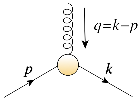
Figure 1: Diagrammatic representation of the dressed quark-gluon vertex $\Gamma_{\mu}(k,p)$ with its momentum flow defined by the incoming quark momentum $p$, the outgoing momentum $k$ and $q=k-p$.

To begin with, as in QED, the fermion-gauge-boson vertex in QCD satisfies a set of constraints imposed by gauge symmetry, multiplicative renormalizability, LKFT as well as the $C$, $P$ and $T$ symmetry properties of the bare vertex; see, for instance, the discussions in Refs. Bashir:2004mu ; Bermudez:2017bpx . Therefore, in a general though not unique decomposition, the fermion-gauge-boson vertex can be written in terms of twelve linearly independent structures Ball:1980ay . In QCD, the STI associated with this vertex is given by,

$$i\,q\cdot\Gamma^{a}(k,p)=G(q^{2})\Big{[}S^{-1}(k)\,H^{a}(k,p)-\bar{H}^{a}(p,k)S^{-1}(p)\Big{]}\ ,$$ (16)

where $q=k-p$ and the momentum flow is depicted in Figure 1 and $S^{-1}(p)=iA(p^{2})\,\gamma\cdot p+B(p^{2})$ is the inverse of the propagator in Eq. 3. The color index $a$ denotes again the implicit SU(3) group generators. The ghost-dressing function $G(q^{2})$ is defined by the ghost propagator,

$$D^{ab}(q^{2})=-\,\delta^{ab}\,\frac{G(q^{2})}{q^{2}}\ ,$$ (17)

renormalized as $G(\mu^{2})=1$, $H^{a}(k,p)=H(k,p)t^{a}$ is the quark-ghost scattering amplitude and $\bar{H}^{a}(p,k)$ is obtained from the conjugate, $H^{\dagger}(-p,-k)$, and the momentum exchange $k\leftrightarrow-p$. This identity allows us to determine the four components of the vertex which are not transverse to the gluon momentum $q$. However, this doesn’t exhaust the number of independent tensor structures that can be formed from the momenta $k$ and $p$ and the Dirac matrices. The full vertex, $\Gamma_{\mu}^{a}(k,p)=\Gamma_{\mu}(k,p)\,t^{a}$ contains additional transverse vertex components and can be decomposed as the sum Ball:1980ay ,

$$\Gamma_{\mu}(k,p)=\Gamma^{L}_{\mu}(k,p)+\Gamma^{T}_{\mu}(k,p)\ .$$ (18)

The transverse vertex $\Gamma^{T}_{\mu}(k,p)$ vertex in Eq. (18) is thus naturally defined by,

$$i\,q\cdot\Gamma^{T}(k,p)=0\,.$$ (19)

The STI (16) constrains the so-called longitudinal vertex, $\Gamma_{L}^{\mu}(k,p)$, to four independent structures,

$$\Gamma^{L}_{\mu}(k,p)=\lambda_{1}(k,p)\,\gamma_{\mu}+\lambda_{2}(k,p)\,\tfrac{1}{2}\,t_{\mu}\,\gamma\cdot t-i\lambda_{3}(k,p)\,t_{\mu}-\lambda_{4}(k,p)\,\sigma_{\mu\nu}t_{\nu}\,,\hskip 11.38109pt$$ (20)

where $t=p+k$ is the sum of the incoming and outgoing quark momenta.

The transverse vertex, ultraviolet-finite at one-loop order Davydychev:2000rt ; Fernandez-Rangel:2016zac , can generally be decomposed into eight independent tensor structures multiplied by associated scalar form factors, $\tau_{i}(k,p)$ Ball:1980ay :

$$\Gamma^{T}_{\mu}(k,p)=\sum_{i=1}^{8}\tau_{i}(k,p)\,T^{i}_{\mu}(k,p)\,.$$ (21)

For the kinematical configuration in Figure 1, the tensors are defined as:

$$T^{1}_{\mu}(k,p) = i\left[p_{\mu}(k\cdot q)-k_{\mu}(p\cdot q)\right]\,,$$ (22)

$$T^{2}_{\mu}(k,p) = \left[p_{\mu}(k\cdot q)-k_{\mu}(p\cdot q)\right]\gamma\cdot t\,,$$ (23)

$$T^{3}_{\mu}(k,p) = q^{2}\gamma_{\mu}-q_{\mu}\,\gamma\cdot q\,,$$ (24)

$$T^{4}_{\mu}(k,p) = iq^{2}\left[\gamma_{\mu}\gamma\cdot t-t_{\mu}\right]+2q_{\mu}p_{\nu}k_{\rho}\sigma_{\nu\rho}\,,$$ (25)

$$T^{5}_{\mu}(k,p) = \sigma_{\mu\,\nu}q_{\nu}\,,$$ (26)

$$T^{6}_{\mu}(k,p) = -\gamma_{\mu}\left(k^{2}-p^{2}\right)+t_{\mu}\,\gamma\cdot q\,,$$ (27)

$$T^{7}_{\mu}(k,p) = \tfrac{i}{2}(k^{2}-p^{2})\left[\gamma_{\mu}\gamma\cdot t-t_{\mu}\right]+t_{\mu}\,p_{\nu}k_{\rho}\sigma_{\nu\rho}\,,$$ (28)

$$T^{8}_{\mu}(k,p) = -i\gamma_{\mu}\,p_{\nu}k_{\rho}\sigma_{\nu\rho}-p_{\mu}\,\gamma\cdot k+k_{\mu}\,\gamma\cdot p\,.\hskip 34.14322pt$$ (29)

Here, we adopt a slightly modified tensor basis Kizilersu:1995iz with respect to the one derived by Ball and Chiu Ball:1980ay . This ensures all transverse form factors are independent of any kinematic singularities in one-loop perturbation theory in an arbitrary covariant gauge.

As discussed in more detail in Refs. Bashir:2004mu ; Bermudez:2017bpx , the fully dressed vertex must exhibit the same properties under charge-conjugation transformation as the bare vertex, which constrains all the $\tau_{i}(k,p)$ in Eq. (21) to be symmetric under the momentum interchange $k\leftrightarrow p$, with the exception of the odd functions $\tau_{4}(k,p)$ and $\tau_{6}(k,p)$:

$$\tau_{i}(k,p) = \tau_{i}(p,k)\,,\quad i=1,2,3,5,7,8$$ (30)

$$\tau_{i}(k,p) = -\tau_{i}(p,k)\,,\quad i=4,6\ .$$ (31)

Similarly, $\lambda_{1}(k,p)$, $\lambda_{2}(k,p)$, $\lambda_{3}(k,p)$ and $\lambda_{4}(k,p)$ are symmetric under $k\leftrightarrow p$, so as to preserve the charge-conjugation properties of the bare vertex.

The STI (16) completely determines the form factors in Eqs. (20) and their expressions are given in In Section 2.3. The transverse scalar functions in Eq. (21), on the other hand, remain undetermined. Nonetheless, as in QED, two additional transverse identities allow to analogously constrain the form of these transverse vertex functions.

2.3 Transverse Slavnov-Taylor identities

A complete fermion-boson vertex based on gauge techniques, such as the one derived from the TTI Qin:2013mta ; Albino:2018ncl , is a first step towards a realistic quark-gluon interaction in QCD valid in any coupling regime. As in QED, gauge invariance as well as Lorentz and charge transformation invariance constrain the tensor structure of the fully dressed three-point function.

As we already saw, the corresponding gauge symmetry preserving relation between Green functions in QCD theory is provided by the STI of Eq. (16), which relates the quark-gluon vertex with the ghost-dressing function, the inverse quark propagator and the quark-ghost scattering kernel, $H(k,p)$, and its conjugate, $\bar{H}(k,p)$. The non-transverse vertex saturates this STI while the transverse vertex is automatically conserved. As in QED, this allows to decompose the fermion-boson vertex into a so-called longitudinal and a transverse part with a tensor basis for which we choose the one defined in Eq. (20) and Eqs (22)–(29). On the other hand, the STI is a consequence of SU(3) gauge invariance and merely makes a statement about the non-transverse components of the vertex. By itself, it fails to ensure gauge covariance in its totality. Under certain simplifying conditions, the WFGTI can be recovered form the STI which leads to an abelianized form of the longitudinal quark-gluon vertex Aguilar:2010cn ; Rojas:2014tya .

How do the DSE solutions of propagators and vertices depend on an arbitrary gauge transformation? In QED the answer to this question can be obtained from the well-defined set of LKFT laws which leave the DSE and WGTI form-invariant. Given a suitable ansatz for the three-point Green function, $\Gamma(k,p)$, that is invariant under a LKFT to another gauge, one can ensure gauge covariance and the WFGTI is satisfied in either gauge. The general rules that govern the LKFT, though, are far from trivial and an extension to the quark propagator in any gauge has only recently been established Aslam:2015nia .

In analogy to QED, the transverse components of the vertex can be constrained by TSTI that relate to the curl of the quark-gluon vertex. Their Dirac structure is identical to that of the TTI and in addition they involve the ghost-dressing function and the quark-ghost scattering kernel. The TSTI can be derived in a functional approach He:2009sj and read:

$$q_{\mu}\Gamma_{\nu}^{a}(k,p)-q_{\nu}\Gamma_{\mu}^{a}(k,p) = G(q^{2})\left[S^{-1}(p)\sigma_{\mu\nu}\,H^{a}(k,p)+\bar{H}^{a}(p,k)\,\sigma_{\mu\nu}S^{-1}(k)\right]$$ (32)

$$+ 2im\,\Gamma_{\mu\nu}^{a}(k,p)+t_{\alpha}\epsilon_{\alpha\mu\nu\beta}\,\Gamma^{5a}_{\beta}(k,p)+A^{a}_{\mu\nu}(k,p)\,,$$

$$q_{\mu}\Gamma^{5a}_{\nu}(k,p)-q_{\nu}\Gamma^{5a}_{\mu}(k,p) = G(q^{2})\left[S^{-1}(p)\sigma^{5}_{\mu\nu}\,H^{a}(k,p)-\bar{H}^{a}(p,k)\,\sigma^{5}_{\mu\nu}S^{-1}(k)\right]$$ (33)

$$+ t_{\alpha}\epsilon_{\alpha\mu\nu\beta}\,\Gamma_{\beta}^{a}(k,p)+V^{a}_{\mu\nu}(k,p)\,,$$

where $m$ is the renormalized current-quark mass in the DSE, $\sigma^{5}_{\mu\nu}=\gamma_{5}\sigma_{\mu\nu}$, and $\Gamma_{\mu\nu}^{a}(k,p)$ is an inhomogeneous tensor vertex. The two tensor structures, $A^{a}_{\mu\nu}$ and $V^{a}_{\mu\nu}$, are Fourier transforms of four-point functions in coordinate space which involve a Wilson line to preserve gauge invariance He:2009sj . Moreover, $\Gamma_{\mu}^{a}(k,p)$ couples to the axialvector vertex via the fourth term on the right-hand side of Eq. (32) and likewise, $\Gamma^{5a}_{\mu}(k,p)$ couples to the vector vertex. We stress that these identities bear no explicit dependence on the covariant gauge parameter. They are valid for any covariant gauge and are not limited to the perturbative case.

We follow Refs. Qin:2013mta ; Albino:2018ncl and proceed in analogous manner to decouple Eqs. (32) and (33). This is done so by introducing the two tensors,

$$T^{1}_{\mu\nu} = \frac{1}{2}\,\epsilon_{\alpha\mu\nu\beta}t^{\alpha}q^{\beta}\,,$$ (34)

$$T^{2}_{\mu\nu} = \frac{1}{2}\,\epsilon_{\alpha\mu\nu\beta}\gamma^{\alpha}q^{\beta}\,.$$ (35)

Contracting the axialvector identity (33) with the tensors (34) and (35) yields zero on the left-hand side of the equation, whereas operating the contractions on the right-hand sides with the identities,

$$T^{1}_{\mu\nu}\,t_{\alpha}\epsilon_{\alpha\mu\nu\beta}\ \Gamma_{\beta}(k,p) = t^{2}q\cdot\Gamma(k,p)-q\cdot t\,t\cdot\Gamma(k,p)\,,$$ (36)

$$T^{2}_{\mu\nu}\,t_{\alpha}\epsilon_{\alpha\mu\nu\beta}\ \Gamma_{\beta}(k,p) = \gamma\cdot t\,q\cdot\Gamma(k,p)-q\cdot t\,\gamma\cdot\Gamma(k,p)\,,$$ (37)

one can recast the two contractions of the axialvector identity into the new form,

$$q\cdot t\,t\cdot\Gamma(k,p) = G(q^{2})\,T^{1}_{\mu\nu}\left[S^{-1}(p)\sigma^{5}_{\mu\nu}\,H(k,p)-\bar{H}(p,k)\sigma^{5}_{\mu\nu}S^{-1}(k)\right]$$ (38)

$$+ t^{2}q\cdot\Gamma(k,p)+T^{1}_{\mu\nu}V_{\mu\nu}\ ,$$

$$q\cdot t\,\gamma\cdot\Gamma(k,p) = G(q^{2})\,T^{2}_{\mu\nu}\left[S^{-1}(p)\sigma^{5}_{\mu\nu}\,H(k,p)-\bar{H}(p,k)\sigma^{5}_{\mu\nu}S^{-1}(k)\right]$$ (39)

$$+ \gamma\cdot t\,q\cdot\Gamma(k,p)+T^{2}_{\mu\nu}V_{\mu\nu}\ ,$$

in which we dropped color indices for simplicity’s sake. Remarkably, these two new identities involve only the vector vertex, $\Gamma_{\mu}(k,p)$, and do not explicitly depend on the quark mass $m$. Likewise, information about the axialvector vertex, $\Gamma^{5}_{\mu}(k,p)$, can be obtained through an analogous procedure involving the vector TSTI (32).

We have thus uncoupled the vector from the axialvector vertex and obtain, in analogy with Ref. Qin:2013mta , three matrix-valued equations for the scalar projections of $\Gamma_{\mu}(k,p)$, namely Eqs. (16), (38) and (39). They form a set of twelve linearly independent and coupled linear equations for the twelve unknown scalar vertex functions, $\lambda_{i}(k,p)$ and $\tau_{i}(k,p)$, which can be solved exactly provided $H^{a}(k,p)$, $\bar{H}^{a}(p,k)$ and $V^{a}_{\mu\nu}(k,p)$ are known. The terms $T^{1}_{\mu\nu}V_{\mu\nu}$ and $T^{2}_{\mu\nu}V_{\mu\nu}$ are unknown objects, yet they are Lorentz-scalar objects which, without loss of generality, can be conveniently expressed as,

$$i\,T^{1}_{\mu\nu}V_{\mu\nu} =Y_{1}(k,p)\mathbbm{1}_{D}+Y_{2}(k,p)\gamma\cdot q+Y_{3}(k,p)\gamma\cdot t+Y_{4}(k,p)\left[\gamma\cdot q,\gamma\cdot t\,\right]\,,$$ (40)

$$i\,T^{2}_{\mu\nu}V_{\mu\nu} =Y_{5}(k,p)\mathbbm{1}_{D}+Y_{6}(k,p)\gamma\cdot q+Y_{7}(k,p)\gamma\cdot t+Y_{8}(k,p)\left[\gamma\cdot q,\gamma\cdot t\,\right]\,,$$ (41)

where $Y_{i}(k,p)$ are hitherto unconstrained scalar functions.

A final ingredient we require to derive the expressions for the form factors $\lambda_{i}(k,p)$ and $\tau_{i}(k,p)$ is the quark-ghost scattering amplitude, $H^{a}(k,p)=H(k,p)t^{a}$, which so far has been studied in a dressed-perturbative approach and will be discussed in more detail in Section 2.4. Nonetheless, employing a similar expedient as in Eqs. (40) and (41), we can decompose the matrix-valued kernel and parameterize it as follows:

$$H(k,p) =X_{0}(k,p)\mathbbm{1}_{D}+X_{1}(k,p)\,\gamma\cdot k+X_{2}(k,p)\,\gamma\cdot p+X_{3}(k,p)\,\left[\gamma\cdot k,\gamma\cdot p\,\right],$$ (42)

$$\ \bar{H}(p,k) =X_{0}(p,k)\mathbbm{1}_{D}-X_{2}(p,k)\,\gamma\cdot k-X_{1}(p,k)\,\gamma\cdot p+X_{3}(p,k)\,\left[\gamma\cdot k,\gamma\cdot p\,\right]\,.$$ (43)

Perturbative expressions for the form factors $X_{i}(k,p)$ are known to one-loop order Davydychev:2000rt and yield $X_{0}(k,p)=1+\mathcal{O}(g^{2})$ and $X_{i}=\mathcal{O}(g^{2})$, $i=1,2,3$. The same diagrammatic approach based on dressed propagators and vertices that incorporate all $X_{i}(k,p)$ form factors in the longitudinal vertex appears to mostly corroborate this dominance, while $X_{3}(k,p)$ may become sizable Aguilar:2016lbe in certain kinematic limits. For the remainder of this work, we make the simplifying assumption that the contribution of $X_{0}(k,p)$ dominates and limit ourselves to the kinematic configuration, $k=q/2$, $p=-q/2\,\Rightarrow\,H(k,p)=H(q/2,-q/2)$, and therefore $X_{0}(k,p)\approx X_{0}(q^{2})$. We neglect sub-leading form factors as their contributions are negligibly small compared to the strength of the transverse vertex, as will be shown shortly.

The decomposition in terms of Lorentz covariants of Eqs. (40), (41), (42) and (43) allows us to write the identities (16), (38) and (39) as a matrix-valued equation system that can be solved by different means. With a set of four projections, with respect to the Dirac trace, one obtains four linearly independent, coupled linear equations whose solutions yield the $\lambda_{i}(k,p)$ form factors and, likewise, the $\tau_{i}(k,p)$ can be isolated using eight different projections. Thus, with the four projections of Eq. (16) we arrive the following scalar vertex functions of the non-transverse vertex:

$$\lambda_{1}(k,p) = \tfrac{1}{2}\,G(q^{2})X_{0}(q^{2})\left[A(k^{2})+A(p^{2})\right]\ ,$$ (44)

$$\lambda_{2}(k,p) = G(q^{2})X_{0}(q^{2})\,\frac{A(k^{2})-A(p^{2})}{k^{2}-p^{2}}\ ,$$ (45)

$$\lambda_{3}(k,p) = G(q^{2})X_{0}(q^{2})\,\frac{B(k^{2})-B(p^{2})}{k^{2}-p^{2}}\ ,$$ (46)

$$\lambda_{4}(k,p) = \ 0\ .$$ (47)

Note that in the absence of the sub-leading $X_{1,2,3}(k,p)$ form factors, $\lambda_{4}(k,p)=0$, as in QED Ball:1980ay . The transverse vertex functions are derived from four projections of each, Eqs. (38) and (39):

$$\tau_{1}(k,p) = -\frac{Y_{1}}{2(k^{2}-p^{2})\nabla(k,p)}\ ,$$ (48)

$$\tau_{2}(k,p) = -\frac{Y_{5}-3Y_{3}}{4(k^{2}-p^{2})\nabla(k,p)}\ ,$$ (49)

$$\tau_{3}(k,p) = \frac{1}{2}\,G(q^{2})X_{0}(q^{2})\left[\frac{A(k^{2})-A(p^{2})}{k^{2}-p^{2}}\right]+\frac{Y_{2}}{4\nabla(k,p)}-\frac{t^{2}(Y_{3}-Y_{5})}{8(k^{2}-p^{2})\nabla(k,p)}\ ,\hskip 28.45274pt$$ (50)

$$\tau_{4}(k,p) = -\frac{6Y_{4}+Y_{6}^{A}}{8\nabla(k,p)}-\frac{t^{2}Y_{7}^{S}}{8(k^{2}-p^{2})\nabla(k,p)}\ ,$$ (51)

$$\tau_{5}(k,p) = -G(q^{2})X_{0}(q^{2})\left[\frac{B(k^{2})-B(p^{2})}{k^{2}-p^{2}}\right]-\frac{2Y_{4}+Y_{6}^{A}}{2(k^{2}-p^{2})}\ ,$$ (52)

$$\tau_{6}(k,p) = \frac{(k-p)^{2}Y_{2}}{4(k^{2}-p^{2})\nabla(k,p)}-\frac{Y_{3}-Y_{5}}{8\nabla(k,p)}\ ,$$ (53)

$$\tau_{7}(k,p) = \frac{q^{2}(6Y_{4}+Y_{6}^{A})}{4(k^{2}-p^{2})\nabla(k,p)}+\frac{Y_{7}^{S}}{4\nabla(k,p)}\ ,$$ (54)

$$\tau_{8}(k,p) = -G(q^{2})X_{0}(q^{2})\left[\frac{A(k^{2})-A(p^{2})}{k^{2}-p^{2}}\right]-\frac{2Y_{8}^{A}}{k^{2}-p^{2}}\ ,$$ (55)

where $Y_{i}\equiv Y_{i}(k,p)$ and the Gram determinant is defined by:

$$\nabla(k,p)=k^{2}p^{2}-(k\cdot p)^{2}\,.$$ (56)

In addition, the vertex transformation properties under charge conjugation determine the symmetry properties of the $Y$-functions:

$$Y_{i}(k,p) = Y_{i}(p,k)\ ,\qquad i=2,6^{S},7^{S},8^{S}\ ,$$ (57)

$$Y_{i}(k,p) = -Y_{i}(p,k)\ ,\quad i=1,3,4,5,6^{A},7^{A},8^{A}\ ,$$ (58)

where, as in Ref. Albino:2018ncl , we introduce the decomposition,

$$Y_{i}(k,p)=Y_{i}^{S}(k,p)+Y^{A}_{i}(k,p)\ ,$$ (59)

for $i=6,7,8$, where the superscripts $S$ and $A$ denote the symmetric and antisymmetric parts of the corresponding $Y_{i}$ functions for $k\leftrightarrow p$. Note that there is no contribution of $Y_{6}^{S}$, $Y_{7}^{A}$ and $Y_{8}^{S}$ to the form factors $\tau_{i}(k,p)$ in Eqs. (48) to (55) as a consequence of the symmetry properties in Eqs. (30) and (31) which imply:

$$Y_{6}^{S}(k,p) = -\frac{(k^{2}-p^{2})Y_{1}(k,p)}{4\nabla(k,p)}\ ,$$ (60)

$$Y_{7}^{A}(k,p) = \frac{q^{2}\,Y_{1}(k,p)}{4\nabla(k,p)}\ ,$$ (61)

$$Y_{8}^{S}(k,p) = -\frac{(k-p)^{2}\,Y_{2}(k,p)}{8\nabla(k,p)}+\frac{(k^{2}-p^{2})Y_{3}(k,p)}{8\nabla(k,p)}\ .$$ (62)

We stress that while Eqs. (44) to (55) are analytic expressions, the remaining challenge stems from our ignorance of the scalar $Y_{i}(k,p)$ functions. We shall constrain their analytical form with an ansatz for the transverse vertex in perturbative QCD Bashir:2011dp in Section 2.5 and postpone the actual calculation of the nontrivial four-point function $V^{a}_{\mu\nu}(k,p)$.

2.4 Quark-ghost scattering amplitude

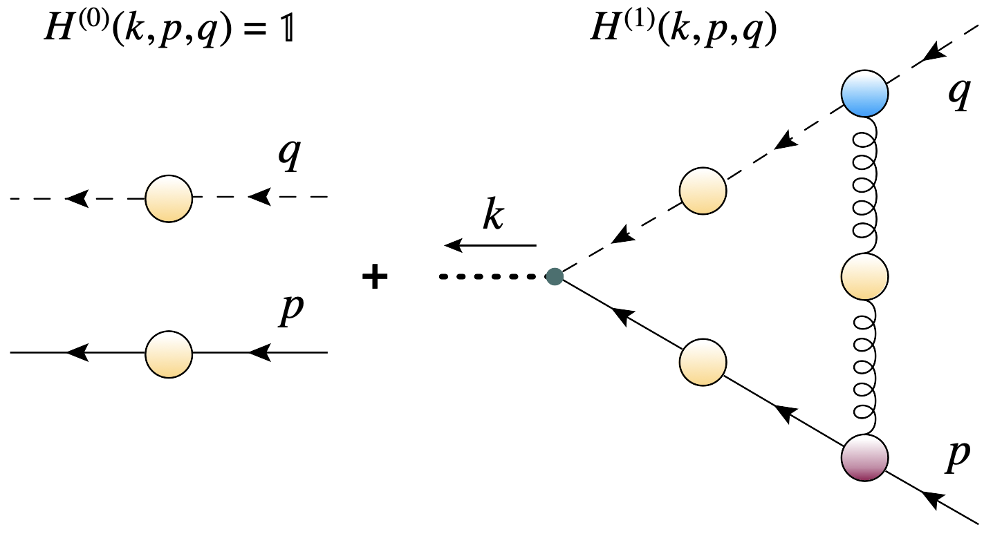
Figure 2: Diagrammatic representation of the unconnected and connected quark-ghost scattering amplitude in its dressed one-loop approximation with the simplified kinematic choice $k=q/2$ and $p=-q/2$. The yellow-shaded circles denote the dressed quark, gluon and ghost propagators, while the blue- and purple-shaded circles represent the dressed ghost-gluon and quark-gluon vertices, respectively. The outgoing quark and ghost propagators are joined in a non-standard “vertex”.

The nonperturbative behavior of the quark-ghost scattering kernel $H^{a}(k,p)$ introduced in the STI (16) is unknown. A tractable ansatz that allows for a connection with the perturbative result Davydychev:2000rt is given by the one-loop dressed approximation to $H^{a}(k,p)$ Aguilar:2010cn , whose diagrammatic representation is depicted in Figure 2. We use the tensorial decomposition of Eqs. (42) and (43) and, as mentioned previously, limit ourself to the dominant form factor $X_{0}(k,p)$ with the momentum configuration $k=q/2$ and $p=-q/2$, so that $X_{0}(q/2,-q/2)\equiv X_{0}(q^{2})$ does not depend on angles. Applying the kinematics of the Feynman diagram in Figure 2, we project out $X_{0}(q^{2})$,

$$X_{0}(q^{2}) =\,\tfrac{1}{4}\operatorname{Tr}_{\mathrm{CD}}H(q/2,-q/2,q)$$

$$=\,1+\frac{C_{A}}{4}\,g^{2}\!\int^{\Lambda}\!\!\frac{d^{4}\ell}{(2\pi)^{4}}\ \Delta_{\mu\nu}(\ell)D(\ell+q)\operatorname{Tr}_{D}\big{[}G_{\nu}\,S\left(\ell+\tfrac{q}{2}\right)\Gamma_{\mu}\left(\ell+\tfrac{q}{2},-\tfrac{q}{2}\right)\!\big{]}\ ,$$ (63)

where $C_{A}=3$ is the Casimir operator in the adjoint representation,

$$G_{\nu}=i\left(\ell_{\nu}+q_{\nu}\right)H_{1}-i\ell_{\nu}\,H_{2}\ ,$$ (64)

is the dressed ghost-gluon vertex and $\ell+q$ and $q$ are respectively the outgoing and incoming ghost momenta, while $\ell$ is the gluon momentum exchanged between the quark and the ghost. Note that that the terms proportional to $\ell_{\mu}$ in the vertex (64) are transverse to the gluon propagator $\Delta_{\mu\nu}(\ell)$ in Landau gauge; $H_{2}$ does therefore not contribute to the quark-ghost kernel. Moreover, the momentum $q$ coincides with the gluon momentum in the gap equation (1).

The remaining form factor $H_{1}(\ell+q,q)\simeq H_{1}(\ell+q,0)\equiv H_{1}(x)$ is parametrized by the expression Dudal:2012zx ,

$$H_{1}(x)=c\left(1+\frac{a^{2}x^{2}}{x^{4}+b^{4}}\right)+(1-c)\,\frac{w^{4}}{w^{4}+x^{4}}\ ,$$ (65)

fitted to lattice-QCD data: $c=1.26$, $a=0.80$ GeV, $b=1.3$ GeV and $w=0.65$ GeV. In Ref. Rojas:2013tza the replacement of the tree-level ghost-gluon vertex by a dressed vertex enhanced $X_{0}(q^{2})$ overall and by about 20% in the peak region $q^{2}=$1–4 GeV². Adding the transverse part of the vertex in the gap equation this observation is not significantly altered. Note that $\Gamma_{\mu}(k,p)=\Gamma^{L}_{\mu}(k,p)+\Gamma^{T}_{\mu}(k,p)$ enters both the DSE (15) and the quark-ghost scattering amplitude in Eq. (63) for consistency.

2.5 Ansatz to constrain the nonlocal Lorentz scalars $T^{1}_{\mu\nu}V_{\mu\nu}$ and $T^{2}_{\mu\nu}V_{\mu\nu}$

The vertex ansatz proposed in Ref. Bashir:2011dp is constrained by two requirements: it provides the multiplicative renormalizability of the fermion propagator and produces a gauge-independent critical coupling for DCSB. The appeal of this ansatz lies in the fact that it is merely expressed in terms of the quark propagator’s scalar and vector functions, $B(p^{2})$ and $A(p^{2})$, respectively. In the particular kinematical configuration $k^{2}\gg p^{2}$, the transverse form factors of this ansatz are given by:

$$\tau_{1}(k,p) = a_{1}\frac{B(k^{2})-B(p^{2})}{(k^{2}+p^{2})(k^{2}-p^{2})}\,,$$ (66)

$$\tau_{2}(k,p) = a_{2}\frac{A(k^{2})-A(p^{2})}{(k^{2}+p^{2})(k^{2}-p^{2})}\,,$$ (67)

$$\tau_{3}(k,p) = a_{3}\frac{A(k^{2})-A(p^{2})}{k^{2}-p^{2}}\,,$$ (68)

$$\tau_{4}(k,p) = a_{4}\frac{B(k^{2})-B(p^{2})}{4k^{2}p^{2}}\,,$$ (69)

$$\tau_{5}(k,p) = -a_{5}\frac{B(k^{2})-B(p^{2})}{k^{2}-p^{2}}\,,$$ (70)

$$\tau_{6}(k,p) = -a_{6}\frac{k^{2}+p^{2}}{(k^{2}-p^{2})^{2}}\left[A(k^{2})-A(p^{2})\right]\,,$$ (71)

$$\tau_{7}(k,p) = -\left[\frac{a_{4}q^{2}}{2k^{2}p^{2}}+\frac{a_{7}}{k^{2}+p^{2}}\right]\frac{B(k^{2})-B(p^{2})}{k^{2}-p^{2}}\,,$$ (72)

$$\tau_{8}(k,p) = a_{8}\frac{A(k^{2})-A(p^{2})}{k^{2}-p^{2}}\,,$$ (73)

where the coefficients $a_{i}$ are unknown constants.

Inserting the above form factors in Eqs. (48) to (55), we derive the following expressions for the $Y_{i}(k,p)$ which consequently depend on the $a_{i}$ coefficients:

$$Y_{1}(k,p) = -2a_{1}\left[B(k^{2})-B(p^{2})\right]\frac{\nabla(k,p)}{k^{2}+p^{2}}\ ,$$ (74)

$$Y_{2}(k,p) = \tfrac{1}{2}\left[A(k^{2})-A(p^{2})\right]\big{\{}(k^{2}-p^{2})\left(G(q^{2})X_{0}(q^{2})-2a_{3}\right)$$ (75)

$$- 2\left(\frac{k^{2}+p^{2}}{k^{2}-p^{2}}\right)(k+p)^{2}a_{6}\Big{\}}\ ,$$

$$Y_{3}(k,p) = \tfrac{1}{2}\left[A(k^{2})-A(p^{2})\right]\big{\{}-q^{2}\left(G(q^{2})X_{0}(q^{2})-2a_{3}\right)$$ (76)

$$+ 4\,\frac{\nabla(k,p)}{k^{2}+p^{2}}a_{2}+2(k^{2}+p^{2})a_{6}\big{\}}\ ,$$

$$Y_{4}(k,p) = -\frac{B(k^{2})-B(p^{2})}{4k^{2}p^{2}(k^{2}+p^{2})}\big{\{}2(k^{2}+p^{2})\nabla(k,p)a_{4}$$ (77)

$$+ 2k^{2}p^{2}(k^{2}+p^{2})\left[a_{5}-G(q^{2})X_{0}\right]+k^{2}p^{2}(k+p)^{2}a_{7}\big{\}}\ ,$$

$$Y_{5}(k,p) = \tfrac{3}{2}\left[A(k^{2})-A(p^{2})\right]\big{\{}-(k-p)^{2}\left[G(q^{2})X_{0}-2a_{3}\right]$$ (78)

$$+ \frac{4}{3}\frac{\nabla(k,p)}{k^{2}+p^{2}}a_{2}+2(k^{2}+p^{2})a_{6}\big{\}}\ ,$$

$$Y_{6}^{A}(k,p) = \frac{B(k^{2})-B(p^{2})}{2k^{2}p^{2}(k^{2}+p^{2})}\big{\{}2(k^{2}+p^{2})\nabla(k,p)a_{4}$$ (79)

$$+ 6k^{2}p^{2}(k^{2}+p^{2})\left(a_{5}-G(q^{2})X_{0}\right)+k^{2}p^{2}(k+p)^{2}a_{7}\big{\}}\ ,$$

$$Y_{7}^{S}(k,p) = a_{7}\left[B(k^{2})-B(p^{2})\right]\frac{k^{2}-p^{2}}{k^{2}+p^{2}}\ ,$$ (80)

$$Y_{8}^{A}(k,p) = -\tfrac{1}{2}\!\left[A(k^{2})-A(p^{2})\right]\!\left(a_{8}+G(q^{2})X_{0}\right)\ .$$ (81)

While the ansatz given by Eqs. (66) to (73) allows us to derive analytic expressions for the $Y_{i}(k,p)$ form factors, we trade our ignorance of their functional form—or of the nonlocal tensor $V_{\mu\nu}$ in general—for that of relative coefficients. The task is now to find a set of solutions $\vec{a}:=\{a_{1},a_{2},a_{3},a_{4},a_{5},a_{6},a_{7},a_{8}\}$ that reproduces mass and wave-function renormalization solutions from lattice QCD or successful phenomenological models employed in calculations of hadron properties. It turns out that this set is rather small since some of the $a_{i}$ are tightly constrained due to multiplicative renormalizability, as we established with the two relations Albino:2018ncl ,

$$a_{2}+2a_{3}-2a_{8} = 0\ ,$$ (82)

$$a_{6} = \frac{1}{2}\ .$$ (83)

As we shall see, DSE solutions are found in the parameter space defined by the intervals, $-2\leq a_{i}\leq+2$. Allowing for the parameters to leave this range mostly leads to unstable or non-converging iterations when solving the integral equations.

3 Gauge sector: gluon and ghost propagators from lattice QCD

We focus on the complete tensor structures of the dressed quark-gluon vertex, in particular on its contribution to DCSB in the gap equation, and, as such, we do not attempt to solve the coupled DSEs for the gluon and the ghost. This exercise is certainly most worthwhile and of particular interest to understand the effect of the vertex in the dressed gluon propagator and its feedback on the quark gap equation. We postpone this more ample and complex study and rather employ the dressed gluon and ghost propagators which have been calculated on the lattice and for which several numerical results are readily available.

We use the following three data sets for the gluon and ghost propagators in Landau gauge obtained with lattice-QCD simulations:

I.

Quenched lattice data by Bogolubsky et al. Bogolubsky:2009dc generated with $\beta=6/g_{0}^{2}=5.70$, a lattice spacing $a=0.17\,$fm and a lattice volume of $L^{4}=(13.6\,\mathrm{fm})^{4}$.

II.

Quenched lattice data for the gluon by Dudal et al. Dudal:2018cli generated with $\beta=6.0$, lattice spacing $a=0.1016(25)\,$fm and two different lattice volumes: $L^{4}=(6.57\,\mathrm{fm})^{4}$ and $L^{4}=(8.21\,\mathrm{fm})^{4}$. Quenched lattice data for the ghost by Duarte et al. Duarte:2016iko generated with $\beta=6.0$, lattice spacing $a=0.1016(25)\,$fm and $L^{4}=(8.128\,\mathrm{fm})^{4}$.

III.

Partially unquenched lattice data by Ayala et al. Ayala:2012pb from the gauge configurations generated by the European Twisted Mass Collaboration (ETMC) for $N_{f}=2+1+1$ with $\beta=1.90$, $(L/a)^{3}\times T/a=32^{3}\times 64$ and $\beta=1.95$, $(L/a)^{3}\times T/a=48^{3}\times 96$.

Each of these three data sets features distinct advantages. The propagators of the sets I and III were calculated with a large lattice volume and the lowest accessible momenta are $p\approx 70\,$MeV and $p\approx 100\,$MeV, while the largest momenta are $p\approx 4\,$GeV and $p\approx 4.5\,$GeV, respectively. Data set III additionally allows us to analyze unquenching effects in the solutions of the quark DSE. The lattice data of set II were obtained with a smaller lattice volume, however for a considerably smaller lattice spacing $a$. Therefore, larger momenta up to $p\approx 7.7\,$GeV are accessible, which provides additional information on the functional behavior in the perturbative domain of these functions.

In exploiting the available lattice data we resort to analytic fits motivated by theoretical considerations. The lattice propagators, $\Delta(q^{2})$ and $G(q^{2})$, of set I and II are parametrized with an expression that combines the refined Gribov-Zwanziger tree-level gluon propagator in the infrared domain supplemented by the 1-loop renormalization group behavior at larger momenta. This amounts to a renormalization-group improved Padé approximation and can be written as Dudal:2018cli

$$\Delta(q^{2})=Z\,\frac{q^{2}+M_{1}^{2}}{q^{4}+M_{2}^{2}q^{2}+M_{3}^{4}}\left[1+\omega\ln\left(\frac{q^{2}+m_{\mathrm{gl}}^{2}}{\Lambda_{\mathrm{QCD}}^{2}}\right)\right]^{\gamma_{\mathrm{gl}}}\ ,$$ (84)

where $\omega=11N_{c}\,\alpha_{s}(\mu)/12\pi$, $\Lambda_{\mathrm{QCD}}=0.425$ GeV and $\gamma_{\mathrm{gl}}=-13/22$ is the 1-loop anomalous gluon dimension. We choose $\mu=4.3$ GeV and $\alpha_{s}=0.3$ Aguilar:2010cn ; Aguilar:2010gm . A least-squares fit yields $\chi^{2}/\mathrm{d.o.f.}=1.788$ for the renormalized gluon-dressing function of set I Bogolubsky:2009dc :

$$Z =1.440\pm 0.003\ , M_{1}^{2} =2.880\pm 0.054\,\mathrm{GeV}^{2}\ ,$$

$$M_{2}^{2} =0.434\pm 0.021\,\mathrm{GeV}^{2}\ , M_{3}^{4} =0.527\pm 0.009\,\mathrm{GeV}^{4}\ ,$$

$$m_{\mathrm{gl}}^{2} =0.305\pm 0.071\,\mathrm{GeV}^{2}\ ,$$ (85)

and in case of set II Dudal:2018cli we obtain $\chi^{2}/\mathrm{d.o.f.}=0.031$ in a best fit to the bare gluon propagator with the parameters,

$$Z =8.421\pm 0.040\ , M_{1}^{2} =2.743\pm 0.184\,\mathrm{GeV}^{2}\ ,$$

$$M_{2}^{2} =0.519\pm 0.073\,\mathrm{GeV}^{2}\ , M_{3}^{4} =0.356\pm 0.029\,\mathrm{GeV}^{4}\ ,$$

$$m_{\mathrm{gl}}^{2} =0.259\pm 0.262\,\mathrm{GeV}^{2}\ ,$$ (86)

where $\Delta(q^{2})$ must be renormalized by a factor $0.3143\,\mu^{2}$. Similarly, we make use of the ghost-dressing parametrization introduced in Ref. Duarte:2016iko ,

$$G(q^{2})=Z\,\frac{q^{4}+M_{2}^{2}q^{2}+M_{1}^{4}}{q^{4}+M_{4}^{2}q^{2}+M_{3}^{4}}\left[1+\omega\ln\left(\frac{q^{2}+\frac{m_{1}^{4}}{q^{2}+m_{0}^{2}}}{\Lambda_{\mathrm{QCD}}^{2}}\right)\right]^{\gamma_{\mathrm{gh}}}\ ,$$ (87)

with the anomalous ghost dimension $\gamma_{\mathrm{gh}}=-9/44$, while $\omega$ and $\Lambda_{\mathrm{QCD}}$ take on the same values as in Eq. 84. Fitting this expression to the ghost propagator of set I Bogolubsky:2009dc renormalized at $\mu=4.3$ GeV we find $\chi^{2}/\mathrm{d.o.f.}=1.534$ and the following parameters:

$$Z =1.059\pm 0.001\ ,\quad M_{1}^{4}=35.562\pm 0.464\,\mathrm{GeV}^{4}\ ,\quad M_{2}^{2}=33.471\pm 0.391\,\mathrm{GeV}^{2}\ ,$$

$$M_{3}^{4} =14.790\pm 0.188\,\mathrm{GeV}^{4}\ ,\quad M_{4}^{2}=29.193\pm 0.331\,\mathrm{GeV}^{2}\ ,\quad m^{2}_{0}=0.018\pm 0.010\,\mathrm{GeV}^{2}\ ,$$

$$m^{4}_{1} =0.001\pm 0.0002\,\mathrm{GeV}^{4}\,.$$ (88)

Likewise, a least-squares fit to the bare ghost propagator of Ref. Duarte:2016iko yields $\chi^{2}/\mathrm{d.o.f.}=0.247$ with the parameter set:

$$Z =5.068\pm 0.086\ ,\quad M_{1}^{4}=19.281\pm 3.685\,\mathrm{GeV}^{4}\ ,\quad M_{2}^{2}=27.721\pm 3.388\,\mathrm{GeV}^{2}\ ,$$

$$M_{3}^{4} =7.695\pm 1.925\,\mathrm{GeV}^{4}\ ,\quad M_{4}^{2}=24.340\pm 2.833\,\mathrm{GeV}^{2}\ ,\quad m^{2}_{0}=0.527\pm 0.083\,\mathrm{GeV}^{2}\ ,$$

$$m^{4}_{1} =0.018\pm 0.021\,\mathrm{GeV}^{4}\,.$$ (89)

Accordingly, $G(q^{2})$ must be renormalized by a factor $4.706$ at $\mu=4.3$ GeV.

On the other hand, we fit the unquenched data in Ref. Ayala:2012pb with a Padé approximant in the region $q\leq q_{0}=3\,$GeV and a renormalization-group improved continuation for $q>q_{0}=3\,$GeV given by

$$\Delta(q^{2}) =\,\frac{\alpha_{1}+\alpha_{2}q^{2}}{\alpha_{3}+\alpha_{4}q^{2}+\alpha_{5}q^{4}}\ , q\leq q_{0}\ ,$$ (90)

$$\Delta(q^{2}) =\,\frac{\alpha_{1}+\alpha_{2}q_{0}^{2}}{\alpha_{3}+\alpha_{4}q_{0}^{2}+\alpha_{5}q_{0}^{4}}\,\frac{q_{0}^{2}}{q^{2}}\left(\frac{\log\left(q_{0}/\Lambda_{\mathrm{QCD}}\right)}{\log\left(q/\Lambda_{\mathrm{QCD}}\right)}\right)^{\!\!\!\frac{\gamma_{\mathrm{gl}}}{\beta}}\ , q>q_{0}\ ,$$ (91)

where the anomalous dimension including flavor dependence is in this case $\gamma_{\mathrm{gl}}=\frac{13}{2}-\frac{2}{3}N_{f}$, $\beta=11-\frac{2}{3}N_{f}$, $N_{f}=4$ and $\Lambda_{\mathrm{QCD}}=600$ MeV. Analogously, the ghost propagator is fitted to the expressions,

$$G(q^{2}) =\,\frac{\beta_{1}+\beta_{2}q^{2}}{\beta_{3}+\beta_{4}q^{2}}\ , q\leq q_{0}\ ,$$ (92)

$$G(q^{2}) =\,\frac{\beta_{1}+\beta_{2}q_{0}^{2}}{\beta_{3}+\beta_{4}q_{0}^{2}}\left(\frac{\log\left(q_{0}/\Lambda_{\mathrm{QCD}}\right)}{\log\left(q/\Lambda_{\mathrm{QCD}}\right)}\right)^{\!\!\!\frac{\gamma_{\mathrm{gh}}}{\beta}}\ , q>q_{0}\ ,$$ (93)

where $\gamma_{\mathrm{gh}}=9/4$. The fitted parameters are pepefit :

$$\alpha_{1} =4.305\;\mathrm{GeV}^{2},\ \ \alpha_{2}=0.979,\ \ \alpha_{3}=1\;\mathrm{GeV}^{4},\ \ \alpha_{4}=1.581\;\mathrm{GeV}^{2},\ \ \alpha_{5}=1.098,$$ (94)

$$\beta_{1} =2.750\;\mathrm{GeV}^{2},\ \ \beta_{2}=1.855\ ,\ \ \beta_{3}=1\;\mathrm{GeV}^{2},\ \ \beta_{4}=1.864\ .$$ (95)

4 Results

4.1 Solving the Dyson-Schwinger equation for real space-like momenta

The DSE (15) is solved by first projecting out the scalar functions $A(p^{2})$ and $B(p^{2})$ of the general solution (3). This yields two coupled, nonlinear integral equations which additionally couple to the integral equation for $X_{0}(q^{2})$ (63). We solve these three equations, $\mathcal{F}(p^{2})=A(p^{2}),B(p^{2})$ and $X_{0}(q^{2})$, simultaneously via an iterative procedure using as convergence criterium,

$$\bm{\epsilon}_{\mathcal{F}}=\dfrac{\left|\mathcal{F}^{n+1}(p^{2})-\mathcal{F}^{n}(p^{2})\right|}{\mathcal{F}^{n}(p^{2})}=10^{-3}\ ,$$ (96)

where $n=20-30$ iterations suffice. Imposing the constraints (82) and (83) we have established the following values for the coefficients $a_{i}$:

$$\centering{\begin{array}[]{c|c|c|c|c|c|c|c}\hline\cr\hline\cr a_{1}&a_{2}&a_{3}&a_{4}&a_{5}&a_{6}&a_{7}&a_{8}\\ \hline\cr 2&2&-1&-1&1&\tfrac{1}{2}&\tfrac{1}{2}&0\\ \hline\cr\hline\cr\end{array}}\@add@centering$$ (97)

The crucial choice is $a_{3}\leq 0$, as positive values of this coefficient inevitably lead to spurious or non-converging solutions of the integral-equation system. With the choice $a_{3}=-1$ and with $a_{6}$ fixed by the condition (83) we then adjust $a_{2}$ and $a_{8}$ to satisfy condition (82). It turns out that the wave-function renormalization, $Z(p^{2})$, is quite sensitive to $a_{8}\neq 0$ and either positive or negative values impact its functional behavior unfavorably in the infrared domain; i.e. $Z(p^{2})$ turns back to its perturbative value $\approx 1$, a feature also observed in conjunction with the Ball-Chiu vertex. A similar observation holds for $a_{4}>0$ and we therefore use $a_{4}=-1$. Thus, setting $a_{8}=0$ we have $a_{2}=2$ while $a_{1}>0$ leads to an increase in the mass function. The solutions exhibit little dependence on the choice for $a_{5}$, whereas $a_{7}<0$ results in a mass function that decreases too fast and yields negative masses at large momenta. We remark that this choice is not unique, but within the constraints of Eqs. (83) and (83) and with the necessary choice of $a_{3}\leq 0$ little room for variation is left as we checked with some $n>200$ configurations.

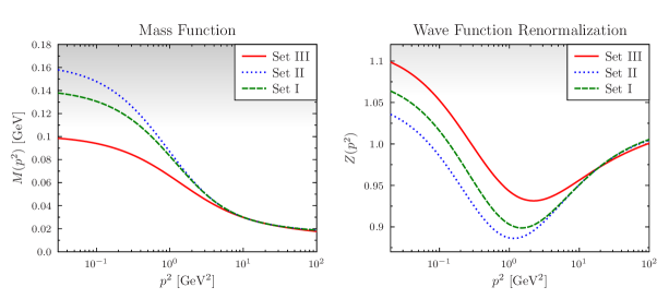
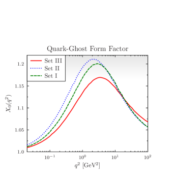
Figure 3: Mass function, $M(p^{2})$, wave renormalization, $Z(p^{2})$, and the quark-ghost kernel form factor, $X_{0}(q^{2})$, for three sets of gluon and ghost propagators, using only $\Gamma_{\mu}^{L}(k,p)$ and the form factors of Eqs. (44)–(47) in the DSE (15). Set I Bogolubsky:2009dc and II Dudal:2018cli ; Duarte:2016iko : $\alpha_{s}(\mu)=0.30$, $m(\mu)=25\,$MeV, $\mu=4.3$  GeV. Set III Ayala:2012pb : $\alpha_{s}(\mu)=0.35$, $m(\mu)=25\,$MeV, $\mu=4.3$  GeV.

Our quark-gluon vertex is now fully determined and in the following we present the solutions for $M(p^{2})$, $Z(p^{2})$ and $X_{0}(q^{2})$ for the three sets of gluon and ghost propagators discussed in Section 3. Note that in what follows we determine $Z_{4}(\mu,\Lambda)$ by imposing $m(\mu)\equiv M(\mu)$ at $\mu=4.3$ GeV. Considering degenerate light-quark masses in the range $m(2\,\mathrm{GeV})\approx$ 30–50 MeV employed in lattice simulations Ayala:2012pb , we choose $m(4.3\,\mathrm{GeV})=25$ MeV. Along with $A(4.3\,\mathrm{GeV})=0.98$, we therefore impose the renormalization conditions:

$$Z_{2}(\mu,\Lambda) = \frac{A(\mu^{2})}{1+\Sigma_{\rm v}(\mu,\Lambda)}\ ,$$ (98)

$$Z_{4}(\mu,\Lambda) = \frac{B(\mu^{2})-Z_{2}(\mu,\Lambda)\,\Sigma_{\rm s}(\mu,\Lambda)}{m(\mu)}\ ,$$ (99)

where $\Sigma_{\rm s}(\mu,\Lambda)$ and $\Sigma_{\rm v}(\mu,\Lambda)$ are the integrals after the usual scalar and vector projections of the right-hand-side of Eq. (15) with $\mathcal{P}_{B}=\mathbbm{1}_{D}/4$ and $\mathcal{P}_{A}=-i\gamma\cdot p/4p^{2}$, respectively:

$$A(p^{2})\ =\ Z_{2}(\mu,\Lambda)+Z_{2}(\mu,\Lambda)\,\Sigma_{\rm v}(p,\Lambda)\ ,$$ (100)

$$B(p^{2})\ =\ Z_{4}(\mu,\Lambda)\,m(\mu)+Z_{2}(\mu,\Lambda)\,\Sigma_{\rm s}(p,\Lambda)\ .$$ (101)

In order to appreciate the effect of the non-transverse components of $\Gamma_{\mu}(k,p)$, we first omit the contributions of $\Gamma_{\mu}^{T}$ following the work of Ref. Rojas:2013tza , however without artificially enhancing $X_{0}(q^{2})$ by an inversion procedure. The mass and wave-renormalization functions along with the form factor $X_{0}(q^{2})$ are plotted in Figure 3 for the gluon and ghost propagator sets discussed in Section 3. The values for $m(\mu)$ and $\alpha_{s}(\mu)$ at the renormalization scale $\mu$ are detailed for each set in Figure 3 and we remark the following: the gluon- and ghost- dressing functions of sets I and II are renormalized at $\mu=4.3\,$ GeV where we employ $\alpha_{s}(\mu)=0.30$ at this scale following Refs. Aguilar:2010cn ; Aguilar:2010gm . We also renormalize the DSE at $\mu=4.3$ GeV when using the unquenched propagators of set III but increase the strong coupling to $\alpha_{s}(\mu)=0.35$, as otherwise only a trivial solution, $M(0)\approx 0$, is found. This is in line with the behavior of the Taylor coupling in Ref. Ayala:2012pb .

The mass functions in Figure 3 exhibit the well-known fast rise at about $p=1$ GeV and saturate at low momenta, where the mass $M(0)$ ranges between 100 MeV and 163 MeV. While these solutions exhibit appreciable DCSB, it is much lower than that obtained with phenomenological models and does not yield the correct pion mass and weak decay constant Bashir:2012fs . The functional behavior of $Z(p^{2})$ is characteristic of that produced with a Ball-Chiu vertex and the Maris-Tandy model Maris:1997tm in the gap equation and indeed, in Eqs. (44) to (47) the longitudinal form factors describe a “ghost-corrected” Ball-Chiu vertex. However, the depth of the minimum of $Z(p^{2})$ is less pronounced than with the phenomenological approach and the growth in the deep infrared is exacerbated with values of $Z(0)>1$. Clearly, limiting the vertex to its non-transverse components yields mass- and wave-renormalization functions which are unlike those required for realistic applications in hadron physics. We note that the leading form factor of the quark-ghost scattering kernel behaves similarly in all three cases with a maximum located around 2–5 GeV² but different magnitudes. Notably, the more enhanced solutions for $X_{0}(q^{2})$ using set I and II are also accompanied by an increased DCSB in the corresponding mass functions. The net contribution of $X_{0}(q^{2})$ to $M(p^{2})$ is 27% when using set I and 29% when using set II; solving the DSE with set III and keeping $X_{0}(q^{2})=1$ does not yield a mass gap.

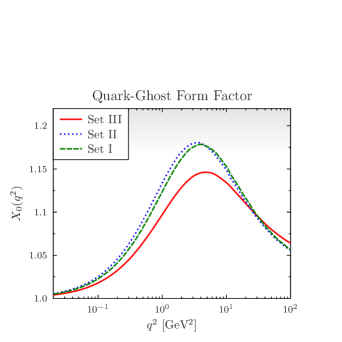
Figure 4: Mass function, $M(p^{2})$, wave renormalization, $Z(p^{2})$, and leading quark-ghost kernel form factor, $X_{0}(q^{2})$, obtained with three sets of gluon and ghost propagators, $\Gamma_{\mu}(k,p)=\Gamma^{L}_{\mu}(k,p)+\Gamma^{T}_{\mu}(k,p)$ and associated form factors of Eqs. (44)–(55) in the DSE (15). Current-quark masses, strong couplings and renormalization scale as in Figure 3.

We now introduce the transverse components of the quark-gluon vertex, $\Gamma_{\mu}(k,p)=\Gamma^{L}_{\mu}(k,p)+\Gamma^{T}_{\mu}(k,p)$, in the DSE and therefore all 12 form factors, Eqs. (44) to (47) and (48) to (55), come into play. The solutions for $M(p^{2})$, $Z(p^{2})$ and $X_{0}(q^{2})$ are again juxtaposed for the three sets of gluon and ghost propagators in Figure 4. We immediately notice the drastic increase of the mass functions, exemplified by $M(0)=500$ MeV for set I, $M(0)=546$ MeV for set II and $M(0)=458$ MeV for set III. In other words, including the transverse vertex leads to a 235%–350% increase in DCSB, while the contribution of the quark-ghost scattering amplitude $X_{0}(q^{2})$ is in the range of 14%–17%. The resulting wave renormalizations likewise exhibit a different behavior at low momenta: while they do not monotonously fall as lattice-QCD calculations indicate, albeit with larger errors at low momenta Oliveira:2016muq , they flatten out and only slightly bend over compared to the solutions obtained with merely the longitudinal vertex. The quark-ghost form factors $X_{0}(q^{2})$ in Figure 4 are similar to those in Figure 3, yet we note that overall their maximum values decrease.

A worthwhile observation is that no solutions for the coupled integral equations (100), (101) and (63) are found if we define $Y_{i}(k,p)\equiv 0$, $i=1,...,8$, regardless of the value of the strong coupling $\alpha_{s}(\mu)$. The same is true if we set $\tau_{4}(k,p)=\tau_{7}(k,p)=0$. Indeed, these two transverse form factors are responsible for the overwhelming contribution to DCSB in the gap equation. Keeping them both and discarding, one by one, the remaining $\tau_{i}(k,p)$, $i=1,2,3,5,6,8$ or combinations thereof, results in very similar solutions. Depending on which form factor is discarded, variations of 5–10% of the mass functions plotted in Figure 4 are observed, some leading to a decrease while others to an increase of $M(p^{2})$. Hence, the form factors other than $\tau_{4}(k,p)$ and $\tau_{7}(k,p)$ are merely responsible for the fine details of the transverse vertex. We note that $\tau_{4}(k,p)$ and $\tau_{7}(k,p)$ are very similar in structure to $Y_{4}(k,p)$, $Y_{6}^{A}(k,p)$ and $Y_{7}^{S}(k,p$), all of which are proportional to the difference of the mass functions, $\Delta B(k,p)=B(k)-B(p)$. On the other hand, if we retain only $\tau_{3}(k,p)$ and $\tau_{5}(k,p)$, which also explicitly depend on $\Delta B(k,p)$, the resulting mass functions exhibit modest DCSB, about 20–30% larger than when the transverse vertex is completely neglected, as depicted in Figure 3.

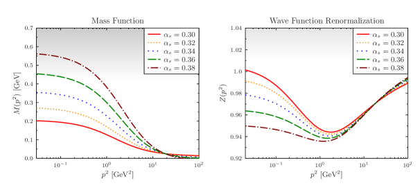
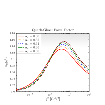
Figure 5: Functional dependence of $M(p^{2})$, $Z(p^{2})$ and $X_{0}(q^{2})$ on the strong coupling $\alpha_{s}$. The DSE (15) is solved with the vertex $\Gamma_{\mu}(k,p)=\Gamma^{L}_{\mu}(k,p)+\Gamma^{T}_{\mu}(k,p)$ and the corresponding form factors in Eqs. (44)–(55); and with the gluon and ghost propagators of set III Ayala:2012pb . The current-quark mass is $m(4.3\,\mathrm{GeV})=25$ MeV.

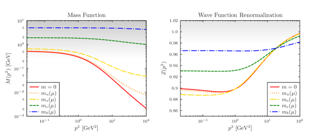
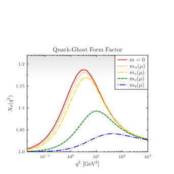
Figure 6: Flavor dependence of $M(p^{2})$, $Z(p^{2})$ and $X_{0}(q^{2})$ obtained with the gluon- and ghost propagators of set II Dudal:2018cli ; Duarte:2016iko . The DSE (15) is solved with the vertex $\Gamma_{\mu}(k,p)=\Gamma^{L}_{\mu}(k,p)+\Gamma^{T}_{\mu}(k,p)$ and the associated form factors in Eqs. (44)–(55). The strong coupling is $\alpha_{s}(\mu)=0.3$ and the current quark masses are: $m_{u,d}(\mu)=25.0$ MeV, $m_{s}(\mu)=82.1$ MeV, $m_{c}(\mu)=1.304$ GeV and $m_{b}(\mu)=4.697$ GeV at the renormalization scale $\mu=4.3$ GeV. For comparison, we also plot the solutions in the chiral limit which define the quark propagators in Eqs. (105) and (106).

The mass functions in Figure 4 clearly demonstrate that the inclusion of the transverse components in the DSE has a dramatic impact on dynamical mass generation. This was already realized long ago and calculations beyond the rainbow-ladder truncation commonly include phenomenological ansätze for several transverse components, in particular those proportional to $\Delta B(k^{2},p^{2})=B(k^{2})-B(p^{2})$. The novelty in this approach is that the present transverse quark-gluon vertex, derived from gauge identities and whose unknown tensor component is constrained with a vertex ansatz motivated by perturbation theory and multiplicative renormalizability Bashir:2011dp , generates copious DCSB without the need to resort to a phenomenological gluon model.

On the other hand, the wave renormalization $Z(p^{2})$ tends to increase again in the infrared region below 1 GeV in case of the gluon and ghost propagators of set I and III. One may wonder whether the strength of the transverse vertex, whose effect flattens out $Z(p^{2})$ at lower momenta, is compatible with what model interactions in given truncation schemes predict. The overall strength of the quark-gluon interaction, however, is controlled by the strong coupling. In using what lattice QCD offers us for the gluon and ghost propagators renormalized at 4.3 GeV, we also work with a strong coupling expected at that renormalization scale. However, given that our transverse vertex has not been determined exactly and that our approach is not self-consistent—we do not solve the gluon and ghost DSE that couple to the quark-gap equation—we may consider variations of $\alpha_{s}$. We do so in Figure 5 where we vary the coupling $\alpha_{s}(4.3\,\mathrm{GeV})$ in the range between 0.30 and 0.38 and concentrate merely on set III of gluon and ghost propagators. Plainly, an increasing coupling strength carries along two modifications: $M(p^{2})$ is enhanced, which is expected, whereas $Z(p^{2})$ is increasingly suppressed and eventually levels out below $p\approx 1$ GeV. The form factor $X_{0}(q^{2})$ is also enhanced as a function of $\alpha_{s}$ and its peak value slightly shifts to larger momenta.

The DSE can obviously also be solved for different quark flavors and we do this exercise in Figure 6, where we make use of the gluon and ghost propagators of set II; the results for the two other sets are qualitatively and quantitatively very similar. We employ the light, strange and charm current-quark masses renormalized at 2 GeV of Ref. Ayala:2012pb : $m_{u}(2\,\mathrm{GeV})=m_{d}(2\,\mathrm{GeV})=40$ MeV, $m_{s}(2\,\mathrm{GeV})=95$ MeV, $m_{c}(2\,\mathrm{GeV})=1.51$ GeV evolved to the scale $\mu=4.3$ GeV. For the bottom quark we choose $m_{b}(4.3\,\mathrm{GeV})=M_{b}(4.3\,\mathrm{GeV})=4.70$ GeV, where $M_{b}(p^{2})$ is the mass function for that flavor obtained with an interaction model Qin:2011dd in rainbow truncation.

The pattern of the mass function for increasing current-quark masses mirrors the well-known behavior predicted by phenomenological gluon and vertex models, see Refs. ElBennich:2012tp ; Serna:2018dwk for example. At $p=0$ GeV we find: $M_{u}(0)=0.55$ GeV, $M_{s}(0)=0.67$ GeV, $M_{c}(0)=1.92$ GeV and $M_{b}(0)=4.97$ GeV. Thus, even for the charm quark the impact of dynamical mass generation is important. The wave renormalization function flattens out in the infrared region for heavier quarks but remains above $Z(0)\approx 0.93$ when $Z(4.3\,\mathrm{GeV})=0.98$ is imposed. We also read from Figure 6 that $X_{0}(q^{2})$ is very sensitive to the current-quark mass and while the function is increasingly damped, its maximum value is considerably shifted to large momenta where it contributes little to DCSB in heavy quarks.

4.2 Solving the Dyson-Schwinger equation on the complex plane

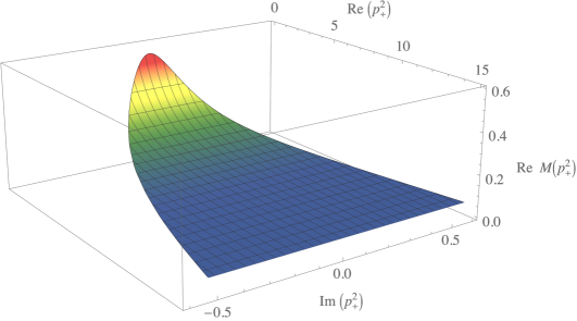
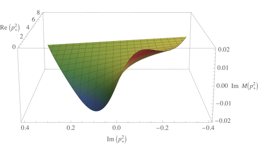
Figure 7: Real part (upper panel) and imaginary part (lower panel) of the complex mass function $M(p^{2})$. The DSE is solved on the complex parabola with $p_{+}$ defined by Eq. (103), the external mass $P^{2}=-M_{\pi}^{2}$ ($M_{\pi}=140$ MeV) and $\eta=1/2$. We use the gluon and ghost propagators of set II Dudal:2018cli ; Duarte:2016iko , the vertex $\Gamma_{\mu}(k,p)=\Gamma^{L}_{\mu}(k,p)+\Gamma^{T}_{\mu}(k,p)$ with the form factors in Eqs. (44)–(47) and (48)–(55), while $\alpha_{s}(\mu)=0.3$. Mass units are in GeV.

So far, we have solved the DSE on the real spacelike axis which suffices to evaluate the magnitude of DCSB and the confining properties of the solutions. However, in solving the bound-state equation in Euclidean space Serna:2017nlr the quark propagators,

$$S(p_{\pm})=-i\gamma\cdot p_{\pm}\,\sigma_{\mathrm{v}}(p_{\pm}^{2})+\sigma_{\mathrm{s}}(p_{\pm}^{2})\ ,$$ (102)

are evaluated at complex-valued momenta. This is because in Euclidean space their arguments, $p_{+}=p+\eta P$ and $p_{-}=p-\bar{\eta}P$, define parabolas on the complex plane,

$$p^{2}_{+}=p^{2}-\eta^{2}M^{2}+2i\eta M|p|z_{p}\ ,$$ (103)

$$p^{2}_{-}=p^{2}-\bar{\eta}^{2}M^{2}-2i\bar{\eta}M|p|z_{p}\ ,$$ (104)

where $P=\big{(}\vec{0},iM\big{)}$ is the meson’s rest-frame momentum, $\eta+\bar{\eta}=1$ are the momentum partition parameters with $\eta,\bar{\eta}\in[0,1]$, and $z_{p}=p\cdot P/|p||P|$ is the angle between the relative and total meson momenta for which $-1\leq z_{p}\leq+1$ holds.

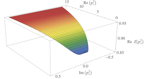
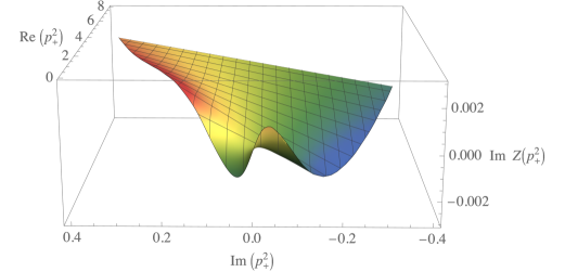
Figure 8: Real part (upper panel) and imaginary part (lower panel) of the complex wave-renormalization function $Z(p^{2})$. Details of the DSE solution as in Figure 7.

We use Cauchy’s integral theorem to solve the quark DSE inside this parabola. At first, we parametrize the contour of the parabola in the lower and upper half of the complex plane and find solutions on this contour via an iterative procedure using the same renormalization procedure as in Eqs. (98) and (99). Then, we apply this contour solution in Cauchy’s integral formula again to find solutions for $\sigma_{\mathrm{v}}(p_{\pm}^{2})$ and $\sigma_{\mathrm{s}}(p_{\pm}^{2})$ inside the parabola. A detailed discussion with examples of parametrizations can be found in Refs. Fischer:2005en ; Krassnigg:2009gd ; Rojas:2014aka .

The real and imaginary parts of the $M(p^{2})$ and $Z(p^{2})$ functions are plotted in Figures 7 and 8, respectively. The real part of $M(p^{2})$ is a smooth and monotonically decreasing function of $p^{2}\equiv p^{2}_{+}$ in real direction, whereas it is all but constant along the imaginary axis $\mathrm{Im}\,(p^{2})$. Likewise, the real part of $Z(p^{2})$ smoothly tends towards its perturbative limit both on and off the real axis. The imaginary part of both functions is characterized by complex-conjugate extrema near the origin of the parabola, though we note that their magnitude is considerably smaller than that of the imaginary parts of solutions with model propagators Maris:1997hd ; Qin:2011dd ; El-Bennich:2020aiq .

Generally speaking, in the complex momentum range considered herein, the two solutions presented in Figures 7 and 8 are qualitatively very similar to those obtained with phenomenological interaction models in rainbow-ladder truncation. There are, on the other hand, distinctive quantitative and analytical differences and we here refrain from a detailed comparison. We merely note that the convergence of the complex DSE using a Cauchy integral, with the present vertex and its inherent complexities, raises subtle issues that depend on the details of the contour parametrization and its size determined by the parabola cutoff on the complex plane.

	Set I	Set II	Set III
$f_{\pi}^{0}$ [MeV]	97.0	96.02	98.67
$(-\langle\bar{q}q\rangle)^{\frac{1}{3}}$ [MeV]	251.16	249.61	255.80

Table 1: Weak decay constant in the chiral limit (105) and quark condensate (106) calculated with the solutions for $M(p^{2})$ and $Z(p^{2})$ using the longitudinal (20) and transverse (21) vertex in the DSE (15) and the three sets of gluon and ghost propagators introduced in Section 3.

4.3 Applications

While the numerical DSE solutions we obtain with the vertex defined by Eqs. (20) and (21) along with Eqs. (44) to (55) lead to typical constituent masses and characteristic mass functions for all flavors considered in Figure 6, only the calculation of a gauge-independent observable can tell us more about how realistic they are. Naturally, the next step consists in the construction of an antiquark-quark Bethe-Salpeter kernel that is consistent with this new vertex and must satisfy the axialvector Ward-Takahashi identities. Given the complexity of the task, we postpone it to a future work.

However, even without the knowledge of the pion’s Bethe-Salpeter amplitude we may compute its weak decay constant, which is a measure of chiral symmetry breaking. Indeed, while the pion’s mass vanishes in chiral limit, $f_{\pi}$ does not. We follow Ref. Roberts:1994hh where the weak decay constant in the chiral limit is expressed by the integral,

$$\left(f_{\pi}^{0}\right)^{\!2}\,=\,\dfrac{N_{c}}{8\pi^{2}}\int_{0}^{\infty}\!dp^{2}p^{2} \,B^{2}(p^{2})\left(\sigma_{\rm v}^{2}-2\left[\sigma_{\rm s}\sigma_{\rm s}^{\prime}+p^{2}\sigma_{\rm v}\sigma_{\rm v}^{\prime}\right]\right.$$

$$\left.-\ p^{2}\left[\sigma_{\rm s}\sigma_{\rm s}^{\prime\prime}-(\sigma_{\rm s}^{\prime})^{2}\right]-p^{4}\left[\sigma_{\rm v}\sigma_{\rm v}^{\prime\prime}-(\sigma_{\rm v}^{\prime})^{2}\right]\right)\ ,$$ (105)

with $\sigma_{\rm s,v}^{\prime}\equiv d\sigma_{\rm s,v}(p^{2})/dp^{2}$. As we are constrained by a low renormalization point due to our use of quenched lattice-QCD input for the gluon and ghost propagators, determining $Z_{2}$ and $Z_{4}$ in the chiral limit is not straightforward. We set $m=0$ MeV at $\mu=4.3$ GeV which allows for a sensible approximation in using $\sigma_{\rm s}(p^{2})$ and $\sigma_{\rm v}(p^{2})$ to calculate the decay constant in the chiral limit.

As another application, we consider the quark condensate which is an order parameter for DCSB. As for the pion decay constant, we do so using the three DSE solutions for the full vertex at hand, i.e. $M(p^{2})$ and $Z(p^{2})$ obtained with the different ghost and gluon-dressing functions in the chiral limit. We thus calculate the integral over the trace of the quark propagator:

$$-\langle\bar{q}q\rangle\,\equiv\,Z_{4}N_{c}\int^{\Lambda}\!\frac{d^{4}k}{(2\pi)^{4}}\,\operatorname{tr}_{D}\left[S(k)\right]\ .$$ (106)

The values of the decay constant $f_{\pi}^{0}$ and of the quark condensate are obtained for all three sets of gluon and ghost propagators and are summarized in Table 1. The three values for $f_{\pi}^{0}$ are slightly above the experimental value, $f_{\pi^{\pm}}=92.2$ MeV, while the quark condensates are in good agreement with other estimates, for instance the chiral condensate in the $\overline{\mathrm{MS}}$ scheme using SU(2) chiral perturbation theory Borsanyi:2012zv , $(-\langle\bar{q}q\rangle)^{1/3}=272(2)$ MeV, or the light-quark condensate from lattice QCD McNeile:2012xh : $(-\langle\bar{q}q\rangle)^{1/3}=283(2)$ MeV.

5 Conclusive remarks and future developments

We have derived a novel form of the transverse quark-gluon vertex that complements the “longitudinal” components obtained as a ghost-corrected Ball-Chiu vertex in Refs. Aguilar:2010cn ; Aguilar:2016lbe ; Aguilar:2018csq ; Rojas:2013tza which saturates the STI Slavnov:1972fg ; Taylor:1971ff . As for the non-transverse components, we were guided by symmetry transformations and multiplicative renormalizability encoded in the set of two TSTI He:2009sj which couple the vector and axialvector vertices. By means of projections with two appropriate tensors one obtains an identity for each of these vertices, i.e. the TSTI have been decoupled.

Once this is realized, one can project out the eight transverse form factors for which we obtain the expressions in Eqs. (48) to (55). Notably, of the twelve form factors that describe the fully dressed quark-gluon vertex, only $\lambda_{1}(k,p)$, $\lambda_{2}(k,p)$, $\lambda_{3}(k,p)$, $\tau_{3}(k,p)$, $\tau_{5}(k,p)$ and $\tau_{8}(k,p)$ depend directly on the quark-ghost kernel and ghost-dressing function. Of course, due to imposing the Bashir-Bermudez ansatz for the transverse vertex to constrain the scalar $Y_{i}(k,p)$ functions, the latter are also functions of the quark-ghost kernel and ghost-dressing function. The last ingredients are the eight parameters, $\vec{a}:=\{a_{1},a_{2},a_{3},a_{4},a_{5},a_{6},a_{7},a_{8}\}$, inherent to the Bashir-Bermudez vertex specified by Eqs. (66) to (73). We showed that they are far from being free parameters, as they are constrained by multiplicative renormalizability relations and limited to a rather narrow range outside of which no or very unsatisfying solutions of the DSE are found.

Nonetheless, while our dressed quark-gluon vertex in its present form is successful in producing the right amount of DCSB for hadron phenomenology, as our results for the weak decay constant of the pion and the quark condensate demonstrate, the reliance on parameters is unsatisfying and theoretically undesirable. Amongst future perspectives, we plan to obtain an integral expression for the four-point function, at the origin of the tensor elements $T^{1}_{\mu\nu}V_{\mu\nu}$ and $T^{2}_{\mu\nu}V_{\mu\nu}$, along similar lines applied to the quark-ghost kernel in Section 2.4. We remind that the nonlocal four-point function is related to the tensor $V_{\mu\nu}$ via the line integral,

$$V_{\mu\nu}=\int\!\frac{d^{4}\ell}{(2\pi)^{4}}\,2\ell_{\lambda}\,\epsilon_{\lambda\mu\nu\rho}\,\Gamma_{\rho}(k,p;\ell)\ ,$$ (107)

where $\Gamma_{\rho}(k,p;\ell)$ is the Fourier transform of the four-point function in coordinate space and which is defined in QED by He:2009sj :

$$\int\!d^{4}x\,d^{4}x^{\prime}d^{4}x_{1}\,d^{4}x_{2} \ e^{i\left(k\cdot x_{1}-p\cdot x_{2}+(p-\ell)\cdot x-(k-\ell)\cdot x^{\prime}\right)}\,\langle 0|T\bar{\psi}(x^{\prime})\gamma_{\rho}\mathcal{W}(x^{\prime},x)\psi(x)\psi(x_{1})\bar{\psi}(x_{2})|0\rangle$$

$$= \ (2\pi)^{4}\delta^{4}(k-p-q)\,S(k)\Gamma_{\rho}(k,p;\ell)S(p)\ ,$$ (108)

with $q=(k-\ell)-(p-\ell)$ and $\mathcal{W}(x^{\prime},x)$ is a Wilson line that ensures a gauge invariant expression. The expression in QCD is analogous, yet involves in addition color matrices and ghost fields. Therefore, expanding the Wilson line to leading order in the strong coupling $g$ Costa:2021mpk , the matrix element can be expressed approximately by diagrams that describe the gluon dressing of quarks, the two-quark scattering and the interaction of a quark with a ghost via gluon exchange. However, in such an approach the propagators ought to be dressed as in the dressed approximation to $H^{a}(k,p)$ discussed in Section 2.4. With this ansatz, one can contract $V_{\mu\nu}$ with the tensors $T^{1}_{\mu\nu}$ and $T^{2}_{\mu\nu}$ to obtain the form factor decomposition of Eqs. (40) and (41) and subsequently project out all $Y_{i}(k,p)$ functions. As a consequence, we arrive at a set of eight integral equations which are all coupled with each other as well as with the integral equations for $A(p^{2})$, $B(p^{2})$ and $X_{0}(q^{2})$ we considered in this work.

In future studies, the quark-ghost kernel we presented in Section 2.4 ought to be calculated beyond the leading approximation that includes only $X_{0}(q^{2})$ and moreover neglects any angular dependence; see Refs. Aguilar:2016lbe ; Aguilar:2018csq for detailed calculations. This is important as $\lambda_{4}(k,p)$ remains otherwise zero and in the particular case of the soft-gluon limit, $k=p$ ($q^{2}=0$), the expressions for $\lambda_{1}(k,p)$ (44) and $\lambda_{2}(k,p)$ (45) hardly express any functional dependence without the full inclusion of the $X_{i}(k,p)$ Oliveira:2020yac . However, for our present purpose this simplified ansatz proves to be sufficient, as our aim was to demonstrate that an important amount of DCSB in the gap equation is due to the transverse quark-gluon vertex. We are therefore optimistic that with future refinements a complete vertex structure can be achieved that catches the dynamical subtleties much beyond the leading truncation, indispensable for the reproduction of the excited hadron spectrum and exotic states.

- (1) S. Aoki et al. [Flavour Lattice Averaging Group], Eur. Phys. J. C 80, no.2, 113 (2020) doi:10.1140/epjc/s10052-019-7354-7
- (2) Y. B. Yang, J. Liang, Y. J. Bi, Y. Chen, T. Draper, K. F. Liu and Z. Liu, Phys. Rev. Lett. 121, no.21, 212001 (2018) doi:10.1103/PhysRevLett.121.212001
- (3) C. D. Roberts and A. G. Williams, Prog. Part. Nucl. Phys. 33, 477-575 (1994) doi:10.1016/0146-6410(94)90049-3
- (4) A. Bashir, L. Chang, I. C. Cloët, B. El-Bennich, Y. X. Liu, C. D. Roberts and P. C. Tandy, Commun. Theor. Phys. 58, 79-134 (2012) doi:10.1088/0253-6102/58/1/16
- (5) I. C. Cloët, G. Eichmann, B. El-Bennich, T. Klähn and C. D. Roberts, Few Body Syst. 46, 1-36 (2009) doi:10.1007/s00601-009-0015-x
- (6) G. Eichmann, R. Alkofer, A. Krassnigg and D. Nicmorus, Phys. Rev. Lett. 104, 201601 (2010) doi:10.1103/PhysRevLett.104.201601
- (7) I. G. Aznauryan, A. Bashir, V. Braun, S. J. Brodsky, V. D. Burkert, L. Chang, C. Chen, B. El-Bennich, I. C. Cloët and P. L. Cole, et al. Int. J. Mod. Phys. E 22, 1330015 (2013) doi:10.1142/S0218301313300154
- (8) J. Segovia, B. El-Bennich, E. Rojas, I. C. Cloët, C. D. Roberts, S. S. Xu and H. S. Zong, Phys. Rev. Lett. 115, no.17, 171801 (2015) doi:10.1103/PhysRevLett.115.171801
- (9) G. Eichmann, C. S. Fischer and H. Sanchis-Alepuz, Phys. Rev. D 94, no.9, 094033 (2016) doi:10.1103/PhysRevD.94.094033
- (10) G. Eichmann, H. Sanchis-Alepuz, R. Williams, R. Alkofer and C. S. Fischer, Prog. Part. Nucl. Phys. 91, 1-100 (2016) doi:10.1016/j.ppnp.2016.07.001
- (11) H. Sanchis-Alepuz and R. Williams, Comput. Phys. Commun. 232, 1-21 (2018) doi:10.1016/j.cpc.2018.05.020
- (12) C. Chen, B. El-Bennich, C. D. Roberts, S. M. Schmidt, J. Segovia and S. Wan, Phys. Rev. D 97, no.3, 034016 (2018) doi:10.1103/PhysRevD.97.034016
- (13) C. Chen, Y. Lu, D. Binosi, C. D. Roberts, J. Rodríguez-Quintero and J. Segovia, Phys. Rev. D 99, no.3, 034013 (2019) doi:10.1103/PhysRevD.99.034013
- (14) K. D. Bednar, I. C. Cloët and P. C. Tandy, Phys. Lett. B 782, 675-681 (2018) doi:10.1016/j.physletb.2018.06.020
- (15) V. V. Flambaum, A. Holl, P. Jaikumar, C. D. Roberts and S. V. Wright, Few Body Syst. 38, 31-51 (2006) doi:10.1007/s00601-005-0123-1
- (16) J. S. Ball and T. W. Chiu, Phys. Rev. D 22, 2542 (1980) doi:10.1103/PhysRevD.22.2542
- (17) A. I. Davydychev, P. Osland and L. Saks, Phys. Rev. D 63, 014022 (2001) doi:10.1103/PhysRevD.63.014022
- (18) C. S. Fischer, A. Maas and J. M. Pawlowski, Annals Phys. 324, 2408-2437 (2009) doi:10.1016/j.aop.2009.07.009
- (19) R. Alkofer, M. Q. Huber and K. Schwenzer, Phys. Rev. D 81, 105010 (2010) doi:10.1103/PhysRevD.81.105010
- (20) D. Dudal, J. A. Gracey, S. P. Sorella, N. Vandersickel and H. Verschelde, Phys. Rev. D 78, 065047 (2008) doi:10.1103/PhysRevD.78.065047
- (21) A. C. Aguilar and A. A. Natale, JHEP 08, 057 (2004) doi:10.1088/1126-6708/2004/08/057
- (22) A. C. Aguilar, D. Binosi and J. Papavassiliou, Phys. Rev. D 78, 025010 (2008) doi:10.1103/PhysRevD.78.025010
- (23) A. C. Aguilar, D. Binosi and J. Papavassiliou, Phys. Rev. D 86, 014032 (2012) doi:10.1103/PhysRevD.86.014032
- (24) A. Cucchieri and T. Mendes, PoS LATTICE2007, 297 (2007) doi:10.22323/1.042.0297
- (25) A. Cucchieri and T. Mendes, Phys. Rev. Lett. 100, 241601 (2008) doi:10.1103/PhysRevLett.100.241601
- (26) O. Oliveira and P. J. Silva, Phys. Rev. D 79, 031501 (2009) doi:10.1103/PhysRevD.79.031501
- (27) M. R. Pennington and D. J. Wilson, Phys. Rev. D 84, 119901 (2011) doi:10.1103/PhysRevD.84.094028
- (28) O. Oliveira and P. J. Silva, Phys. Rev. D 86, 114513 (2012) doi:10.1103/PhysRevD.86.114513
- (29) I. L. Bogolubsky, E. M. Ilgenfritz, M. Müller-Preussker and A. Sternbeck, Phys. Lett. B 676, 69-73 (2009) doi:10.1016/j.physletb.2009.04.076
- (30) A. Ayala, A. Bashir, D. Binosi, M. Cristoforetti and J. Rodríguez-Quintero, Phys. Rev. D 86, 074512 (2012) doi:10.1103/PhysRevD.86.074512
- (31) S. Strauss, C. S. Fischer and C. Kellermann, Phys. Rev. Lett. 109, 252001 (2012) doi:10.1103/PhysRevLett.109.252001
- (32) A. K. Cyrol, L. Fister, M. Mitter, J. M. Pawlowski and N. Strodthoff, Phys. Rev. D 94, no.5, 054005 (2016) doi:10.1103/PhysRevD.94.054005
- (33) P. Boucaud, F. De Soto, K. Raya, J. Rodríguez-Quintero and S. Zafeiropoulos, Phys. Rev. D 98, no.11, 114515 (2018) doi:10.1103/PhysRevD.98.114515
- (34) B. W. Mintz, L. F. Palhares, G. Peruzzo and S. P. Sorella, Phys. Rev. D 99, no.3, 034002 (2019) doi:10.1103/PhysRevD.99.034002
- (35) D. Dudal, O. Oliveira and P. J. Silva, Annals Phys. 397, 351-364 (2018) doi:10.1016/j.aop.2018.08.019
- (36) A. G. Duarte, O. Oliveira and P. J. Silva, Phys. Rev. D 94 (2016) no.1, 014502 doi:10.1103/PhysRevD.94.014502
- (37) A. C. Aguilar, F. De Soto, M. N. Ferreira, J. Papavassiliou, J. Rodríguez-Quintero and S. Zafeiropoulos, Eur. Phys. J. C 80, no.2, 154 (2020) doi:10.1140/epjc/s10052-020-7741-0
- (38) M. Q. Huber, Phys. Rev. D 91, no.8, 085018 (2015) doi:10.1103/PhysRevD.91.085018
- (39) M. Q. Huber, Phys. Rev. D 101, 114009 (2020) doi:10.1103/PhysRevD.101.114009
- (40) C. S. Fischer and M. Q. Huber, Phys. Rev. D 102, no.9, 094005 (2020) doi:10.1103/PhysRevD.102.094005
- (41) A. F. Falcão, O. Oliveira and P. J. Silva, Phys. Rev. D 102, no.11, 114518 (2020) doi:10.1103/PhysRevD.102.114518
- (42) P. Maris and C. D. Roberts, Phys. Rev. C 56, 3369 (1997) doi:10.1103/PhysRevC.56.3369
- (43) P. Maris, C. D. Roberts and P. C. Tandy, Phys. Lett. B 420, 267 (1998) doi:10.1016/S0370-2693(97)01535-9
- (44) P. Maris and P. C. Tandy, Phys. Rev. C 60, 055214 (1999) doi:10.1103/PhysRevC.60.055214
- (45) R. Alkofer, P. Watson and H. Weigel, Phys. Rev. D 65 (2002), 094026 doi:10.1103/PhysRevD.65.094026
- (46) S. x. Qin, L. Chang, Y. x. Liu, C. D. Roberts and D. J. Wilson, Phys. Rev. C 84, 042202 (2011) doi:10.1103/PhysRevC.84.042202
- (47) L. Chang and C. D. Roberts, Phys. Rev. C 85, 052201 (2012) doi:10.1103/PhysRevC.85.052201
- (48) E. Rojas, B. El-Bennich and J. P. B. C. de Melo, Phys. Rev. D 90, 074025 (2014) doi:10.1103/PhysRevD.90.074025
- (49) K. Raya, L. Chang, A. Bashir, J. J. Cobos-Martínez, L. X. Gutiérrez-Guerrero, C. D. Roberts and P. C. Tandy, Phys. Rev. D 93, no.7, 074017 (2016) doi:10.1103/PhysRevD.93.074017
- (50) B. El-Bennich, G. Krein, E. Rojas and F. E. Serna, Few Body Syst. 57, no.10, 955-963 (2016) doi:10.1007/s00601-016-1133-x
- (51) F. F. Mojica, C. E. Vera, E. Rojas and B. El-Bennich, Phys. Rev. D 96, no.1, 014012 (2017) doi:10.1103/PhysRevD.96.014012
- (52) F. E. Serna, B. El-Bennich and G. Krein, Phys. Rev. D 96 (2017) no.1, 014013 doi:10.1103/PhysRevD.96.014013
- (53) M. A. Bedolla, J. J. Cobos-Martínez and A. Bashir, Phys. Rev. D 92 (2015) no.5, 054031 doi:10.1103/PhysRevD.92.054031
- (54) M. A. Bedolla, K. Raya, J. J. Cobos-Martínez and A. Bashir, Phys. Rev. D 93 (2016) no.9, 094025 doi:10.1103/PhysRevD.93.094025
- (55) K. Raya, M. A. Bedolla, J. J. Cobos-Martínez and A. Bashir, Few Body Syst. 59 (2018) no.6, 133 doi:10.1007/s00601-018-1455-y
- (56) C. S. Fischer, S. Kubrak and R. Williams, Eur. Phys. J. A 51 (2015), 10 doi:10.1140/epja/i2015-15010-7
- (57) T. Hilger, M. Gómez-Rocha, A. Krassnigg and W. Lucha, Eur. Phys. J. A 53 (2017) no.10, 213 doi:10.1140/epja/i2017-12384-4
- (58) P. J. Gunkel, C. S. Fischer and P. Isserstedt, Eur. Phys. J. A 55, no.9, 169 (2019) doi:10.1140/epja/i2019-12868-1
- (59) B. El-Bennich, J. P. B. C. de Melo, B. Loiseau, J. P. Dedonder and T. Frederico, Braz. J. Phys. 38 (2008), 465-471 doi:10.1590/S0103-97332008000400016
- (60) B. El-Bennich, M. A. Ivanov and C. D. Roberts, Nucl. Phys. B Proc. Suppl. 199 (2010), 184-190 doi:10.1016/j.nuclphysbps.2010.02.026
- (61) B. El-Bennich, EPJ Web Conf. 172, 02005 (2018) doi:10.1051/epjconf/201817202005
- (62) B. El-Bennich, C. D. Roberts and M. A. Ivanov, PoS QCD-TNT-II, 018 (2012) doi:10.22323/1.136.0018
- (63) M. Atif Sultan, K. Raya, F. Akram, A. Bashir and B. Masud, Phys. Rev. D 103 (2021) no.5, 054036 doi:10.1103/PhysRevD.103.054036
- (64) F. E. Serna, C. Chen and B. El-Bennich, Phys. Rev. D 99, no.9, 094027 (2019) doi:10.1103/PhysRevD.99.094027
- (65) F. E. Serna, R. C. da Silveira, J. J. Cobos-Martínez, B. El-Bennich and E. Rojas, Eur. Phys. J. C 80 (2020) no.10, 955 doi:10.1140/epjc/s10052-020-08517-3
- (66) M. Gómez-Rocha, T. Hilger and A. Krassnigg, Few Body Syst. 56 (2015) no.6-9, 475-480 doi:10.1007/s00601-014-0938-8
- (67) M. Gómez-Rocha, T. Hilger and A. Krassnigg, Phys. Rev. D 92 (2015) no.5, 054030 doi:10.1103/PhysRevD.92.054030
- (68) M. Gómez-Rocha, T. Hilger and A. Krassnigg, Phys. Rev. D 93 (2016) no.7, 074010 doi:10.1103/PhysRevD.93.074010
- (69) C. S. Fischer and R. Alkofer, Phys. Rev. D 67, 094020 (2003) doi:10.1103/PhysRevD.67.094020
- (70) R. Alkofer, C. S. Fischer, F. J. Llanes-Estrada and K. Schwenzer, Annals Phys. 324, 106-172 (2009) doi:10.1016/j.aop.2008.07.001
- (71) M. Hopfer, A. Windisch and R. Alkofer, PoS ConfinementX, 073 (2012) doi:10.22323/1.171.0073
- (72) R. Williams, Eur. Phys. J. A 51, no.5, 57 (2015) doi:10.1140/epja/i2015-15057-4
- (73) R. Williams, C. S. Fischer and W. Heupel, Phys. Rev. D 93, no.3, 034026 (2016) doi:10.1103/PhysRevD.93.034026
- (74) D. C. Curtis and M. R. Pennington, Phys. Rev. D 42 (1990), 4165-4169 doi:10.1103/PhysRevD.42.4165
- (75) A. Bashir and M. R. Pennington, Phys. Rev. D 50 (1994), 7679-7689 doi:10.1103/PhysRevD.50.7679
- (76) A. Bashir and M. R. Pennington, Phys. Rev. D 53 (1996), 4694-4697 doi:10.1103/PhysRevD.53.4694
- (77) A. Bashir and A. Raya, Nucl. Phys. B 709 (2005), 307-328 doi:10.1016/j.nuclphysb.2004.12.010
- (78) A. Bashir and A. Raya, [arXiv:hep-ph/0411310 [hep-ph]].
- (79) A. Kızılersü and M. R. Pennington, Phys. Rev. D 79, 125020 (2009) doi:10.1103/PhysRevD.79.125020
- (80) A. Bashir, A. Raya and S. Sánchez-Madrigal, Phys. Rev. D 84, 036013 (2011) doi:10.1103/PhysRevD.84.036013
- (81) A. Bashir, R. Bermudez, L. Chang and C. D. Roberts, Phys. Rev. C 85, 045205 (2012) doi:10.1103/PhysRevC.85.045205
- (82) M. J. Aslam, A. Bashir and L. X. Gutiérrez-Guerrero, Phys. Rev. D 93, no.7, 076001 (2016) doi:10.1103/PhysRevD.93.076001
- (83) L. A. Fernández-Rangel, A. Bashir, L. X. Gutiérrez-Guerrero and Y. Concha-Sanchez, Phys. Rev. D 93, no.6, 065022 (2016) doi:10.1103/PhysRevD.93.065022
- (84) R. Bermudez, L. Albino, L. X. Gutiérrez-Guerrero, M. E. Tejeda-Yeomans and A. Bashir, Phys. Rev. D 95, no.3, 034041 (2017) doi:10.1103/PhysRevD.95.034041
- (85) L. Albino, A. Bashir, L. X. Gutiérrez-Guerrero, B. El-Bennich and E. Rojas, Phys. Rev. D 100, no.5, 054028 (2019) doi:10.1103/PhysRevD.100.054028
- (86) E. Rojas, J. P. B. C. de Melo, B. El-Bennich, O. Oliveira and T. Frederico, JHEP 10, 193 (2013) doi:10.1007/JHEP10(2013)193
- (87) E. Rojas, B. El-Bennich, J. P. B. C. De Melo and M. A. Paracha, Few Body Syst. 56, no. 6-9, 639 (2015) doi:10.1007/s00601-015-1020-x
- (88) S. X. Qin, L. Chang, Y. X. Liu, C. D. Roberts and S. M. Schmidt, Phys. Lett. B 722, 384-388 (2013) doi:10.1016/j.physletb.2013.04.034
- (89) D. Binosi, L. Chang, J. Papavassiliou, S. X. Qin and C. D. Roberts, Phys. Rev. D 95, no. 3, 031501 (2017). doi:10.1103/PhysRevD.95.031501
- (90) A. C. Aguilar and J. Papavassiliou, Phys. Rev. D 83, 014013 (2011) doi:10.1103/PhysRevD.83.014013
- (91) A. C. Aguilar, D. Binosi, D. Ibañez and J. Papavassiliou, Phys. Rev. D 90, no.6, 065027 (2014) doi:10.1103/PhysRevD.90.065027
- (92) A. C. Aguilar, J. C. Cardona, M. N. Ferreira and J. Papavassiliou, Phys. Rev. D 96, no.1, 014029 (2017) doi:10.1103/PhysRevD.96.014029
- (93) A. C. Aguilar, J. C. Cardona, M. N. Ferreira and J. Papavassiliou, Phys. Rev. D 98, no.1, 014002 (2018) doi:10.1103/PhysRevD.98.014002
- (94) A. C. Aguilar, M. N. Ferreira, C. T. Figueiredo and J. Papavassiliou, Phys. Rev. D 99, no.3, 034026 (2019) doi:10.1103/PhysRevD.99.034026
- (95) S. Jia and M. R. Pennington, Phys. Rev. D 94, no.11, 116004 (2016) doi:10.1103/PhysRevD.94.116004
- (96) O. Oliveira, W. de Paula, T. Frederico and J. P. B. C. de Melo, Eur. Phys. J. C 79, no.2, 116 (2019) doi:10.1140/epjc/s10052-019-6617-7
- (97) O. Oliveira, T. Frederico and W. de Paula, Eur. Phys. J. C 80, no.5, 484 (2020) doi:10.1140/epjc/s10052-020-8037-0
- (98) A. Bashir, A. Kızılersü and M. R. Pennington, Phys. Rev. D 57, 1242-1249 (1998) doi:10.1103/PhysRevD.57.1242
- (99) A. Bashir, A. Kızılersü and M. R. Pennington, [arXiv:hep-ph/9907418 [hep-ph]].
- (100) A. Bashir, A. Kızılersü and M. R. Pennington, Phys. Rev. D 62, 085002 (2000) doi:10.1103/PhysRevD.62.085002
- (101) M. Peláez, M. Tissier and N. Wschebor, Phys. Rev. D 92, no.4, 045012 (2015) doi:10.1103/PhysRevD.92.045012
- (102) J. Skullerud and A. Kızılersü, JHEP 09, 013 (2002) doi:10.1088/1126-6708/2002/09/013
- (103) J. I. Skullerud, P. O. Bowman, A. Kızılersü, D. B. Leinweber and A. G. Williams, JHEP 04, 047 (2003) doi:10.1088/1126-6708/2003/04/047
- (104) A. Kızılersü, D. B. Leinweber, J. I. Skullerud and A. G. Williams, Eur. Phys. J. C 50, 871-875 (2007) doi:10.1140/epjc/s10052-007-0250-6
- (105) O. Oliveira, A. Kızılersu, P. J. Silva, J. I. Skullerud, A. Sternbeck and A. G. Williams, Acta Phys. Polon. Supp. 9, 363-368 (2016) doi:10.5506/APhysPolBSupp.9.363
- (106) A. Sternbeck, P. H. Balduf, A. Kızılersü, O. Oliveira, P. J. Silva, J. I. Skullerud and A. G. Williams, PoS LATTICE2016, 349 (2017) doi:10.22323/1.256.0349
- (107) A. Kızılersü, O. Oliveira, P. J. Silva, J. I. Skullerud and A. Sternbeck, Phys. Rev. D 103, no.11, 114515 (2021) doi:10.1103/PhysRevD.103.114515
- (108) J. C. Ward, Phys. Rev. 78, 182 (1950) doi:10.1103/PhysRev.78.182
- (109) E. S. Fradkin, Zh. Eksp. Teor. Fiz. 29, 258-261 (1955)
- (110) H. S. Green, Proc. Phys. Soc. A 66, 873-880 (1953) doi:10.1088/0370-1298/66/10/303
- (111) Y. Takahashi, Nuovo Cim. 6, 371 (1957) doi:10.1007/BF02832514
- (112) Y. Takahashi, Print-85-0421 (ALBERTA).
- (113) K. I. Kondo, Int. J. Mod. Phys. A 12, 5651-5686 (1997) doi:10.1142/S0217751X97002978
- (114) H. X. He, F. C. Khanna and Y. Takahashi, Phys. Lett. B 480, 222-228 (2000) doi:10.1016/S0370-2693(00)00353-1
- (115) H. X. He, Commun. Theor. Phys. 46, 109-112 (2006) doi:10.1088/0253-6102/46/1/025
- (116) H. X. He, Int. J. Mod. Phys. A 22, 2119-2132 (2007) doi:10.1142/S0217751X07036257
- (117) M. R. Pennington and R. Williams, J. Phys. G 32, 2219-2234 (2006) doi:10.1088/0954-3899/32/11/014
- (118) H. x. He and F. C. Khanna, Int. J. Mod. Phys. A 21, 2541-2551 (2006) doi:10.1142/S0217751X06029533
- (119) L. D. Landau and I. M. Khalatnikov, Sov. Phys. JETP 2, 69 (1956)
- (120) A. A. Slavnov, Theor. Math. Phys. 10, 99 (1972) [Teor. Mat. Fiz. 10, 153 (1972)]. doi:10.1007/BF01090719
- (121) J. C. Taylor, Nucl. Phys. B 33, 436 (1971) doi:10.1016/0550-3213(71)90297-5
- (122) H. x. He, Phys. Rev. D 80, 016004 (2009) doi:10.1103/PhysRevD.80.016004.
- (123) T. De Meerleer, D. Dudal, S. P. Sorella, P. Dall’Olio and A. Bashir, Phys. Rev. D 97 (2018) no.7, 074017 doi:10.1103/PhysRevD.97.074017
- (124) T. De Meerleer, D. Dudal, S. P. Sorella, P. Dall’Olio and A. Bashir, Phys. Rev. D 101 (2020) no.8, 085005 doi:10.1103/PhysRevD.101.085005
- (125) A. Kizilersu, M. Reenders and M. R. Pennington, Phys. Rev. D 52 (1995), 1242-1259 doi:10.1103/PhysRevD.52.1242
- (126) C. Itzykson and J. B. Zuber, “Quantum Field Theory”, New York, USA: Mcgraw-Hill (1980) 705 p. (International Series In Pure and Applied Physics).
- (127) W. J. Marciano and H. Pagels, Phys. Rept. 36 (1978), 137 doi:10.1016/0370-1573(78)90208-9
- (128) P. Boucaud, F. De Soto, J. P. Leroy, A. Le Yaouanc, J. Micheli, O. Pene and J. Rodríguez-Quintero, Phys. Rev. D 79, 014508 (2009) doi:10.1103/PhysRevD.79.014508
- (129) A. C. Aguilar, D. Binosi and J. Papavassiliou, JHEP 07, 002 (2010) doi:10.1007/JHEP07(2010)002
- (130) D. Dudal, O. Oliveira and J. Rodríguez-Quintero, Phys. Rev. D 86 (2012), 105005 doi:10.1103/PhysRevD.86.105005
- (131) J. Rodríguez-Quintero, private communication.
- (132) C. S. Fischer, P. Watson and W. Cassing, Phys. Rev. D 72 (2005), 094025 doi:10.1103/PhysRevD.72.094025
- (133) A. Krassnigg, PoS CONFINEMENT8 (2008), 075 doi:10.22323/1.077.0075
- (134) C. D. Roberts, Nucl. Phys. A 605, 475-495 (1996) doi:10.1016/0375-9474(96)00174-1
- (135) B. El-Bennich, G. Ramos-Zambrano and E. Rojas, Phys. Rev. D 103, no.7, 076008 (2021) doi:10.1103/PhysRevD.103.076008
- (136) S. Borsanyi, S. Durr, Z. Fodor, S. Krieg, A. Schäfer, E. E. Scholz and K. K. Szabo, Phys. Rev. D 88, 014513 (2013) doi:10.1103/PhysRevD.88.014513
- (137) C. McNeile, A. Bazavov, C. T. H. Davies, R. J. Dowdall, K. Hornbostel, G. P. Lepage and H. D. Trottier, Phys. Rev. D 87, no.3, 034503 (2013) doi:10.1103/PhysRevD.87.034503
- (138) C. S. R. Costa, A. Freese, I. C. Cloët, B. El-Bennich, G. Krein and P. C. Tandy, Phys. Rev. C 104, no.4, 045201 (2021) doi:10.1103/PhysRevC.104.045201