Misalignment vs Topology in Axion-Like Models

Abstract

Cosmological axions, an important dark matter candidate, are generated when a scalar field with a spontaneously broken $O(2)$ invariance develops an explicitly $O(2)$-breaking tilt cosmologically, leading to coherent production of long-wavelength modes which could be dark matter. It appears that the production efficiency of this mechanism is low, despite possible production from topological structures. To understand this better, we examine production in $O(N)$ generalizations. In particular we highlight the importance of how fast the explicit $O(N)$-breaking potential turns on.

1 Introduction

The QCD axion Weinberg:1977ma ; Wilczek:1977pj is a hypothetical particle which is effectively the angular degree of freedom of a scalar field with a spontaneously broken $O(2)$ symmetry, when there is also an extremely small explicit breaking of the symmetry (making the axion a pseudo-Goldstone boson). It represents a nearly ideal dark matter candidate Preskill:1982cy ; Abbott:1982af ; Dine:1982ah . One scenario for a cosmological abundance of axions to develop Davis:1986xc , recently argued to be the most likely to occur Visinelli:2009zm ; Visinelli:2014twa , is that the $O(2)$ symmetry is restored during or after inflation, and then spontaneously breaks early in the Universe’s history, leading to a network of axionic strings which disappear when the explicit breaking becomes important. A key feature is that the explicit breaking, due to anomalous couplings to QCD, “turns on” rather abruptly as the Universe cools; in the relevant temperature range around 1 GeV, we expect the axion mass to scale as $m_{a}^{2}\propto T^{-7.6}$ Wantz:2009mi ; Borsanyi:2016ksw .

Many authors have investigated the production of axions under these circumstances, both analytically Harari:1987ht ; Hagmann:1998me ; Battye:1993jv ; Battye:1994au , and by using classical field theory simulations on a spacetime lattice Yamaguchi:1998gx ; Yamaguchi:1999yp ; Hiramatsu:2010yu ; Hiramatsu:2012gg ; axion1 ; axion2 . The most reliable approach is to follow the full dynamics of the Axion field and string network as it breaks up and to count the total axions at the end, further improving the reliability of the simulation by incorporating additional physics which accounts for the large string tension associated with short-distance effects along string cores axion4 . These simulations, which are supported by other recent large-scale simulations Vaquero:2018tib ; Buschmann:2019icd , indicate surprisingly that the total axion production is actually less than the expected baseline production efficiency, the so-called misalignment value. Here the misalignment value is the number of axions which would be produced if the Universe consisted of many independent regions, each with an independent, random, and homogeneous starting value on the vacuum manifold of the $O(2)$ model before the explicit breaking became important.

Many people, including these authors, find this result bizarre and counterintuitive. A field with large inhomogeneities, including highly energetic topological defects, somehow generates fewer excitations than it would if it were locally uniform. We want to understand this result better by seeing whether something similar happens in closely related models. In this paper we will investigate what happens if, rather than a two-component scalar field with spontaneously and also very weakly explicitly broken $O(2)$ invariance, we have an $O(N)$ field with $N=3,4,5$. The case $N=3$ also contains topological defects – global monopoles Kibble:1976sj – and $N=4$ has textures Turok:1989ai . But field-theoretical simulations of these models are more reliable than for the case of $O(2)$, because the energies associated with these topological objects are not dominated by their cores but are instead dominated by longer-range field gradients which should be correctly described by a lattice implementation. Therefore the small lattice-spacing limit can be addressed robustly, and our results should be secure.

In Section 2 we will set up the scenario we consider. Then Section 3 describes our numerical implementation of $O(N)$ theory with spontaneous and weak explicit breaking on the lattice, from the initial conditions through to counting axions at the end. Section 4 presents our results, and we end with a discussion. But here we will give a very brief precis of our results. The production of angular (axion-like) excitations is highly sensitive to how suddenly the explicit symmetry breaking turns on with time. If the explicit breaking turns on very abruptly, the field gradients are not very important and the misalignment estimate is fairly accurate. If the breaking turns on slowly, for instance, if the physical (as opposed to conformal) mass is constant, then theories with many field components produce substantially more angular excitations than in the misalignment mechanism. Therefore the very abrupt turn-on of the axion mass in cosmology may be key to understanding why the resulting axion abundance is so modest.

2 Axion-like models

We will describe the axion model and its generalization to $N$ components first by expressing the model, then by outlining its cosmological evolution, and then by showing how nontrivial topological structures play a role in the evolution, and why they are under better control for the case $N\geq 3$ than for $N=2$.

2.1 Field content

For the purposes of cosmology, an axion field can be summarized as a two-component scalar field model $\Phi=(\Phi_{1},\Phi_{2})$ with an $O(2)$ symmetry which is spontaneously broken and also very weakly explicitly broken. The Lagrangian density is

$$-\mathcal{L}_{\mathrm{axion}}=\frac{1}{2}\sum_{i=1}^{2}\partial^{\mu}\Phi_{i}\partial_{\mu}\Phi_{i}+\frac{\lambda}{8}\left(\sum_{i=1}^{2}\Phi_{i}^{2}-f_{a}^{2}\right)^{2}-m_{a}^{2}f_{a}\Phi_{1},$$ (1)

where the $\Phi_{i}$ are two real fields and the choice of explicit symmetry breaking in the $\Phi_{1}$ direction is an arbitrary choice. Temporarily considering the case without explicit symmetry breaking, $m_{a}^{2}=0$, the spontaneous-symmetry-breaking potential selects a vacuum manifold with $\sqrt{\Phi_{1}^{2}+\Phi_{2}^{2}}=f_{a}$, and we can bring out the physics by writing in terms of radial and angular variables: $\Phi_{i}=(|\Phi|\cos(\theta_{\mathrm{a}}),|\Phi|\sin(\theta_{\mathrm{a}}))$, with $|\Phi|=\sqrt{\Phi_{1}^{2}+\Phi_{2}^{2}}$ and $\theta_{\mathrm{a}}=\mathrm{atan}(\Phi_{2}/\Phi_{1})$. The minimum of the axion potential is then achieved whenever $|\Phi|=f_{a}$, and the free choice of $\theta_{\mathrm{a}}$ parametrizes the vacuum manifold. We then distinguish radial excitations $|\Phi|=f_{a}+h$, with $h$ the radial (Higgs or saxion) fluctuation, and angular or axion excitations $a=f_{a}\,\theta_{\mathrm{a}}$. The radial mass is given by $m_{r}^{2}=\lambda f_{a}^{2}$ while the axions are massless before introducing explicit symmetry breaking. When explicit symmetry breaking is present, the global potential minimum lies at approximately $(h,a)=(0,0)$ and the axion mass is given by $m_{a}^{2}$. The value of the symmetry breaking scale can be constrained from cosmological observations, and in the physically interesting regime there is a clear separation of scales given by radial and axion mass, $m_{r}\sim 10^{30}m_{a}$ such that we do not need to consider radial dynamics Turner:1989vc ; Raffelt:1990yz ; Raffelt:1999tx except in the cores of topological defects (see below). In a cosmological setting the angular excitations will have wavelengths of order of the Hubble scale and amplitudes of order 1 radian, representing quantum occupancies of order $f_{a}^{2}/H^{2}$. For typical applications this is $\mathcal{O}(10^{60})$, making a classical field approximation very well justified.

This model can immediately be generalized to $N$-component scalar fields with spontaneously broken $O(N)$ invariance plus a very weak explicit breaking. The Lagrangian density is

$$-\mathcal{L}=\frac{1}{2}\sum_{i=1}^{N}\partial^{\mu}\Phi_{i}\partial_{\mu}\Phi_{i}+\frac{\lambda}{8}\left(\sum_{i=1}^{N}\Phi_{i}^{2}-f_{a}^{2}\right)^{2}-m_{a}^{2}f_{a}\Phi_{1}.$$ (2)

Instead of a single angular variable $\theta_{\mathrm{a}}$ we now have $N-1$ angular variables corresponding to the $N-1$ Goldstone modes of spontaneous $O(N)\to O(N-1)$ breaking. When $m_{a}^{2}\neq 0$ the true minimum resides at $\Phi_{1}=f_{a}$ and $\Phi_{2,\ldots,N}=0$, the angular excitations correspond at linearized order to the $\Phi_{2,\ldots N}$ excitations, and they all have mass-squared values equal to $m_{a}^{2}$.

An important feature of the axion model in cosmology is that the axion mass squared $m_{a}^{2}$ is not directly a Lagrangian mass, but is rather an effect due to nontrivial interactions with the QCD sector. As such it is strongly temperature dependent above $T=200\>\mathrm{MeV}$, which is the regime where the most interesting dynamics will occur. Therefore we are interested in cases where $m_{a}^{2}$ shows a strong temperature dependence. Even though we are not aware of cases where this is relevant for an $O(N)$ model, we will consider similar temperature dependence when we generalize to these models, because our goal is to understand how this among other things affects the final particle number generation.

2.2 Cosmological evolution

Next we consider how the $O(2)$ model and its $O(N)$ generalization would behave cosmologically, with a focus on the final excitation density. If symmetry is restored at some point in the early Universe and then breaks spontaneously, different space regions will rapidly reach the vacuum manifold $|\Phi|=f_{a}$ but will randomly select different angles $\theta_{\mathrm{a}}$. Subsequent (dissipative) dynamics tend to align the value of $\theta_{\mathrm{a}}$ over causally connected regions of space, in order to minimize the gradient energy; the field undergoes local ordering dynamics. However, causality prevents this ordering from occurring globally; two points with non-overlapping past light cones cannot have correlated field values.

We are concerned with evolution in the radiation-dominated early universe, which features a time-varying scale factor $a$ with a Hubble scale $H=\dot{a}/a=1/2t$. We will work in comoving coordinates $x_{i}$ and conformal time $\tau$, so the spacetime metric is

$$g_{\mu\nu}=\left(\frac{\tau}{\tau_{0}}\right)^{2}\eta_{\mu\nu}\,,\quad\eta_{\mu\nu}=\mathrm{Diag}[-1,1,1,1]\,.$$ (3)

The Lagrangian density is then

$$-\sqrt{-g}\>\mathcal{L}=\tau^{2}\left(\frac{1}{2}\sum_{i}\eta^{\mu\nu}\partial_{\mu}\Phi_{i}\partial_{\nu}\Phi_{i}+\frac{\lambda\tau^{2}}{8\tau_{0}^{2}}\left(\sum_{i}\Phi_{i}^{2}-f_{a}^{2}\right)^{2}-\frac{\tau^{2}m_{a}^{2}f_{a}}{\tau_{0}^{2}}\Phi_{i}\right).$$ (4)

The explicit factor of $\tau^{2}$ in front will give rise to Hubble damping, while the extra $\tau^{2}$ factor attached to $m_{a}^{2}$ makes the mass more time dependent in these conformal-time coordinates. We will call the combination $\tau^{2}m_{a}^{2}/\tau_{0}^{2}\equiv m_{a,\mathrm{c}}^{2}$ in what follows. In addition, $m_{a}^{2}$ will have explicit temperature, and therefore time, dependence. Within the axion model this arises because $m_{a}^{2}$ arises from a coupling to QCD dynamics which is temperature dependent; we have (see for instance diCortona:2015ldu ) $m_{a}^{2}=\chi(T)/f_{a}^{2}$ with $\chi(T)$ the QCD topological susceptibility. Instanton gas estimates suggest $m_{a}^{2}\propto T^{-6.7}\propto\tau^{6.7}$ Wantz:2009it but more recent lattice studies find a still stronger dependence, $m_{a}^{2}\propto T^{-7.6}\propto\tau^{7.6}$ Borsanyi:2016ksw . We will parametrize this with a coefficient $n$: $m_{a}^{2}\propto T^{-n}\propto\tau^{n}$, with fixed physical mass being $n=0$ and the axion case being close to $n=7.6$; we will use $n=7$ to represent this case in what follows, and we will contrast the field behavior in these two cases, $n=0$ ($m_{a,\mathrm{c}}^{2}\propto\tau^{2}$) and $n=7$ ($m_{a,\mathrm{c}}^{2}\propto\tau^{9}$).

So long as $m_{a,\mathrm{c}}^{2}\tau^{2}<1$, there is no time for the explicit symmetry breaking to play a role in the dynamics. The field takes values all over its vacuum manifold, the value varies with a spatial coherence length comparable to the system’s age, and there is no useful definition of angular particle number. However, $m_{a,\mathrm{c}}^{2}\tau^{2}\propto\tau^{n+4}$ and one rather abruptly enters the opposite regime where the explicit symmetry breaking is important. Once this happens, the fields are drawn to the unique minimum of the potential. After some complicated dynamics, at late times the field will settle near the global minimum, but with residual spatially inhomogeneous small-angle oscillations.

Once these oscillations truly become small, $\Delta\Phi_{i}^{2}\ll f_{a}^{2}$, one can define a particle number which is an adiabatic invariant in the dual small-angle and $m_{a,\mathrm{c}}^{2}\tau^{2}\gg 1$ approximations. In terms of the Fourier spectrum of the fields $\Phi_{i}(k)$, this invariant is

$$n_{\mathrm{ax}}=\frac{\tau^{2}}{2}\int\frac{\differential[3]{k}}{(2\pi)^{3}}\left(\sqrt{m_{a,\mathrm{c}}^{2}+k^{2}}\sum_{i=2}^{N}\Phi^{2}_{i}(k)+\frac{\sum_{i=2}^{N}\dot{\Phi}^{2}_{i}(k)}{\sqrt{m_{a,\mathrm{c}}^{2}+k^{2}}}\right)$$ (5)

where the factor $\tau^{2}$ in front counteracts the loss of particle number due to Hubble damping. In standard space and time coordinates the corresponding particle number (without the $\tau^{2}$ factor) diminishes as $a^{-3}$, staying fixed per comoving volume, and corresponds to the axion number density in the universe. Our goal will be to determine $n_{\mathrm{ax}}$ and to understand how it depends on the number of field components.

2.3 The misalignment estimate

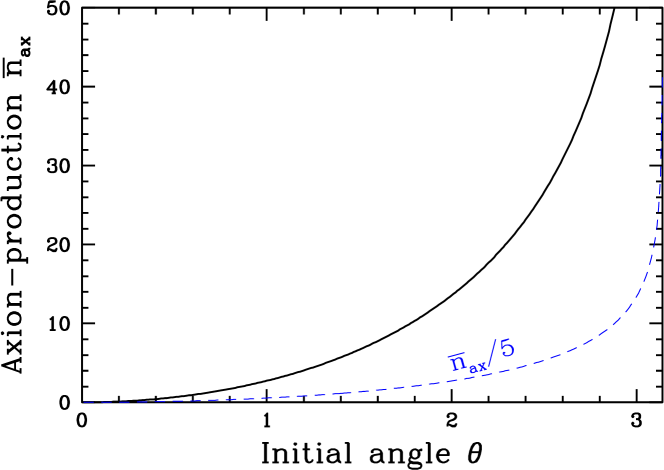
Figure 1: How the axion production efficiency depends on the starting misalignment angle. The curve is quadratic for small angles, but rises towards a logarithmic divergence at $\theta_{\mathrm{a}}=\pi$.

It is useful to begin with a very crude estimate for the final axion density. Consider what dynamics would occur if the field were spatially homogeneous. Consider first the 2-component field. In this case $\theta_{\mathrm{a}}$ starts with some initial value $\theta_{\mathrm{a}}\in[-\pi,\pi]$ and vanishing time derivative (due to Hubble damping). Neglecting gradient terms in the equations of motion, the field evolves according to:

$$\partial_{\tau}^{2}\theta_{\mathrm{a}}+\frac{2}{\tau}\partial_{\tau}\theta_{\mathrm{a}}+m_{a,\mathrm{c}}^{2}\sin(\theta_{\mathrm{a}})=0.$$ (6)

Numerically integrating this equation, one rather easily finds the final (comoving) axion density for each initial $\theta_{\mathrm{a}}$ value: $n_{\mathrm{ax}}(\theta_{\mathrm{a}})$. We plot the $\theta_{\mathrm{a}}$ dependence, for $n=7.6$, in Figure 1. The misalignment estimate is to replace the true field dynamics with random initial conditions with the above dynamics, but average the final axion production uniformly over the range of possible initial $\theta_{\mathrm{a}}$ values: $n_{\mathrm{ax}}=\frac{1}{\pi}\int_{0}^{\pi}n_{\mathrm{ax}}(\theta_{\mathrm{a}})\differential{\theta_{\mathrm{a}}}$. This does not correspond to the axion production in any physical scenario, but it sets a reasonable baseline expectation for axion production for the random phase case.

The generalization to $N$ field components is straightforward. The field begins somewhere on $S^{N-1}$ the $N-1$-sphere. But we can perform an $SO(N-1)$ rotation about the $\Phi_{1}$ axis to place the field excitation entirely in the $(\Phi_{1},\Phi_{2})$ plane. Since the initial time derivatives are zero and $SO(N-1)$ invariance remains unbroken, the field values will stay in this plane and the dynamics are identical to the two-component case. All that changes is the weighting of the initial angle: we now have

$$n_{\mathrm{ax}}[SO(N)]=\frac{\int_{0}^{\pi}n_{\mathrm{ax}}(\theta_{\mathrm{a}})\sin^{N-2}(\theta_{\mathrm{a}})\differential{\theta_{\mathrm{a}}}}{\int_{0}^{\pi}\sin^{N-2}(\theta_{\mathrm{a}})\differential{\theta_{\mathrm{a}}}}\,.$$ (7)

This weights the integral more heavily near $\theta_{\mathrm{a}}=\pi/2$. Since the function is concave, the larger $N$ is, the fewer axions are predicted. More field components lead to fewer excitations!

2.4 Topological objects and their role

We remarked already that the detailed dynamics of field ordering can be complex. One thing which makes them particularly complex is the presence of topological objects, at least for $N=2,3,4$. Here we will give a very quick review; the topic is well addressed in the existing literature Kibble:1976sj ; Vilenkin:1981sd ; Vilenkin:1982ks ; Turok:1989ai ; Bennett:1990xy ; Preskill:1992ck .

We already remarked that the field evolution and the presence of gradient energies leads to locally smooth but globally random fields during the early dynamics, $m_{a,\mathrm{c}}\tau\leq 1$. Such a field configuration generically features topological defects Kibble:1976sj . For an $N$-component field, the vacuum manifold is $S^{N-1}$. Removing a $3-N$ dimensional curve from space – or a $4-N$ dimensional curve from spacetime – leaves a region where the field can vary nontrivially around the vacuum manifold. For $N=2$ one removes a line (or curve) and the field can wind around the circle as one goes around the line. For $N=3$ one removes a point, and the spherical surface enclosing the point can have the field direction on $S^{2}$ wrap nontrivially. In each case, the field must leave the vacuum manifold very close to the removed line/point; the size of this “core” is of order the inverse radial mass $m_{r}^{-1}$. Since the physical case corresponds to $H/m_{r}\sim 10^{-30}$ but on the lattice we can only obtain $H/m_{r}\sim 10^{3}$, the size of this core region is exaggerated on the lattice.

To assess the importance of the mistreatment of the defect core size, we need to estimate how large a role the core plays in the defect’s energetics. The field gradient at a distance $r$ from the defect core is of order $|\nabla\Phi|\sim f_{a}/r$, leading to an energy which scales as

$$E \sim\int_{m_{r}^{-1}}^{H^{-1}}rdr\frac{f_{a}^{2}}{r^{2}}\propto\ln(m_{r}/H)\,, N=2$$ (string) (8)

$$E \sim\int_{m_{r}^{-1}}^{H^{-1}}r^{2}dr\frac{f_{a}^{2}}{r^{2}}\propto H^{-1}-m_{r}^{-1}\,, N=3 \;\mbox{(monopole)}.$$

For $N=2$, the short-distance behavior near the string plays a major role in the energetics and the defect energy scales logarithmically with $m_{r}$; but for $N=3$, the short-distance behavior plays a minor role, with the core energy scaling with $m_{r}^{-1}$. Therefore, using an unphysically small $m_{r}$ value could lead to logarithmically large errors for $N=2$, but the errors will be suppressed by $m_{r}^{-1}$ for $N=3$ and higher. This is why we expect the lattice treatment of $N\geq 3$ to be reliable up to power-suppressed effects, unlike in the case $N=2$ where it is necessary to turn to effective descriptions to capture the relevant string-core physics axion3 ; axion4 .

After explicit symmetry breaking becomes relevant, the defects are no longer strictly topological, since the field now has a unique global minimum. For $N=2$ each string is attached to a domain wall with tension $\sigma=8f_{a}^{2}m_{a}$. The domain wall is locally stable because the gradient energy scales as the inverse wall thickness while the potential energy is linear in the wall thickness. The wall exerts a force-per-length on the attached string, which pulls the string network shut. The associated dynamics play a large role in the energy budget. In contrast, for $N=3$ each monopole is attached to a “string” in whose core $\Phi_{1}=-f_{a}$. However such a string is not locally stable; the gradient energy is independent of the string’s thickness while the potential energy grows with the string thickness, so the string tends to collapse to zero thickness and fragment. Therefore the monopole network can annihilate without the monopoles needing to physically travel to reach each other, and again the finite $m_{r}$ value does not play much of a role in the system’s energetics. The conclusion is that, for $N\geq 3$, topological structures can play a role but they are well described provided that the ratios $m_{r}/m_{a}$, $m_{r}/H$ are large.

2.5 What do we expect?

For any $N\geq 2$, we can follow the dynamics of the theory described by Eq. (4) with $m_{a,\mathrm{c}}^{2}=\tau_{*}^{-2}(\tau/\tau_{*})^{n+2}$. Here $\tau_{*}$ is the scale where $m_{a,\mathrm{c}}(\tau_{*})\tau_{*}=1$, that is, the point where the explicit symmetry breaking first becomes relevant. The axion production $n_{\mathrm{ax}}$ scales on dimensional grounds as $n_{\mathrm{ax}}\propto f_{a}^{2}\tau_{*}$, so we define a dimensionless measure of axion production efficiency

$$\bar{n}_{\mathrm{ax}}\equiv\frac{n_{\mathrm{ax}}}{f_{a}^{2}\tau_{*}}.$$ (9)

What can we say intuitively about the expected behavior for this quantity?

• For the case where $n$ is small, so the explicit symmetry breaking turns on gradually, we might expect that fluctuations in the fields lead to extra axion production. The more field components, the more fluctuations there are in the fields, and so the large-$N$ case should intuitively produce more axions than for small $N$.

• For the case where $n$ is large, the axion mass turns on rather abruptly. In this case, the field rather suddenly finds itself with a large mass. Locally the mass may become larger than the field’s inverse coherence length – that is, the potential energy from the tilted potential may exceed gradient energies – and field gradients and gradient energies would then play little role in the subsequent field oscillations. In this case we would actually expect the misalignment estimate to be fairly close to the actual behavior.

• According to the misalignment mechanism estimate, $\bar{n}_{\mathrm{ax}}$ is the largest for small $N$, that is, few field components.

Intuitively, then, we might expect that for small $n$, the axion production substantially exceeds the misalignment estimate and is larger at larger $N$, while for large $n$ (a rapid turn-on of explicit symmetry breaking), the misalignment estimate is rather close to the true behavior and the axion production gets smaller as we consider theories with more field components.

3 Numerical approach

Here we present our numerical implementation and our extraction of continuum results from lattice calculations.

3.1 Lattice implementation

For numerical simulations, we need to discretise the equations of motion that result from Equation (4) and express them in terms of suitable dimensionless quantities. The equation of motion for the field $\Phi_{j}$, $j=1,\ldots,N$, is

$$0=\left[\partial_{\tau}^{2}+\frac{2}{\tau}\partial_{\tau}-\gradient^{2}+\left(\frac{\tau}{\tau_{0}}\right)^{2}\frac{\lambda}{2}\left(\sum_{i}\Phi_{i}^{2}-f_{a}^{2}\right)\right]\Phi_{j}-m_{a,\mathrm{c}}^{2}f_{a}\delta_{j1}\,.$$ (10)

For easier notation and to make the fields dimensionless, we rescale $\Phi_{i}\longrightarrow\Phi_{i}/f_{a}$, which corresponds to scaling the vacuum manifold to the unit $N-1$-Sphere, additionally requiring the redefinition $\lambda\longrightarrow\lambda f_{a}^{2}$. For the numerical evolution of the fields to be stable for a significant dynamic range, one leaves out the extra scaling of $\tau^{2}$ in front of $\lambda$. This means that the radial mass is then not fixed in “physical” mass but rather in conformal mass, thus fixing the size of monopole cores in terms of lattice units rather than accounting for them growing smaller due to hubble expansion until the lattice could not resolve these defects any more. This is sensible if the goal is to understand the behavior when the core size is very small, and in particular we want in the end to extrapolate to the limit $m_{r}\tau_{*}\gg 1$, which is more easily accomplished with this treatment. For the axion mass, on the other hand, the $\tau^{2}$ scaling is physically relevant and we keep it:

$$m_{a,\mathrm{c}}^{2}=m_{a}^{2}\frac{\tau^{2}}{\tau_{*}^{2}}=\frac{1}{\tau_{*}^{2}}\left(\frac{\tau}{\tau_{*}}\right)^{n+2}\qquad\mbox{and}\qquad\lambda\equiv m_{r}^{2}\,.$$ (11)

We shall investigate the “axion-like” case of $n=7$ and compare it to the constant physical mass case of $n=0$. We lattice discretize the equation of motion with a leapfrog scheme, except that we use backwards differences for the single $\tau$-derivative. This is still consistent with an $a^{2}$-accurate algorithm because this term is suppressed by a $1/\tau$ leading coefficient. Explicitly, our update rule is:

$$\begin{split}\Phi_{i}(\tau+\operatorname{a_{\tau}},x)=&\,2\Phi_{i}(\tau,x)-\Phi(\tau-\operatorname{a_{\tau}},x)-\frac{2\operatorname{a_{\tau}}}{\tau}\left(\Phi_{i}(\tau,x)-\Phi_{i}(\tau-\operatorname{a_{\tau}},x)\right)\\ &+\operatorname{a_{\tau}^{2}}\sum_{j=1}^{3}\frac{\Phi_{i}(\tau,x+\operatorname{a_{x}}_{j})+\Phi_{i}(\tau,x-\operatorname{a_{x}}_{j})-2\Phi_{i}(\tau,x)}{\operatorname{a_{x}^{2}}}\\ &-\operatorname{a_{\tau}^{2}}\operatorname{a_{x}^{2}}\frac{m_{r}^{2}}{2}\left(\sum_{i}\Phi_{i}(\tau,x)^{2}-1\right)\Phi_{i}+\delta_{j1}\frac{\operatorname{a_{\tau}^{2}}}{\tau_{*}^{2}}\left(\frac{\tau}{\tau_{*}}\right)^{n+2}.\end{split}$$ (12)

Because $\Phi(\tau-\operatorname{a_{\tau}})$ is only used locally, we can directly replace $\Phi(\tau-\operatorname{a_{\tau}})$ with $\Phi(\tau+\operatorname{a_{\tau}})$ in memory, so our memory footprint is the field values on two time slices. We simulate on a cubic box of size $L=N_{x}\operatorname{a_{x}}$ with $N_{x}$ some integer and impose periodic boundary conditions. This emulates behavior on an unbounded volume as long as $\tau<\frac{L}{2}$, which is when the lightlike signals from an event near $\tau=0$ can first encounter each other around the periodicity. If the speed of information propagation is lower than the speed of light, then this threshhold is respectively increased. The implementation is written in C++ using AVX512 intrinsics and OMP for parallelisation. Initial values are generated by randomly sampling an $N$-tuple from a unit gaussian distribution and rescaling to the vacuum manifold at each lattice site. For pseudo-random number generation we use the PCG Random C++ header library, which in particular is well suited for providing multiple streams of random numbers for parallel use. Using the update formula we can now numerically evolve the axion fields and then subsequently extract the axion number. We do this by implementing Eq. (5) and Eq. (9), using the FFTW package for C++ as an efficient implementation of the Fourier transform. To optimize the Fourier transform efficiency, we work on cubic lattices with $N_{x}=1024$, 1536, and 2048. Since the particle number depends both on $\Phi$ and on $\dot{\Phi}$, we compute $\dot{\Phi}$ using the difference between two time slices; the $\Phi$-dependent part is computed on each time slice and averaged.

We can also use our code to evaluate $\bar{n}_{\mathrm{ax}}$ in the misalignment approximation, simply by leaving out the middle line of Eq. (12), which removes the gradient term and turns the code into an independent evolution at each lattice site. Then we also need to replace $\sqrt{k^{2}+m^{2}}\to m$ in Eq. (5). We checked that this results in the same $\bar{n}_{\mathrm{ax}}$ result as we get by using an adaptive differential equation solver to evaluate Eq. (6), evaluating $n_{\mathrm{ax}}(\theta_{\mathrm{a}})$, and numerically integrating Eq. (7).

3.2 Late-time, large-mass, continuum extrapolations

The previous subsection shows how to numerically evaluate $\bar{n}_{\mathrm{ax}}$ for a given number of field components $N$ and mass evolution $n$, at a given value of three lattice parameters; the final time $\tau/\tau_{*}$, the radial mass in physical units $m_{r}\tau_{*}$, and the lattice spacing in terms of the radial mass $m_{r}\operatorname{a_{x}}$. Of these, $N$ and $n$ represent distinct physical problems which we want to understand. But the other three parameters are nuissance lattice parameters whose influences must be extrapolated away; the desired physical result requires the joint limits $\tau/\tau_{*}\to\infty$, $m_{r}\tau_{*}\to\infty$, and $m_{r}\operatorname{a_{x}}\to 0$. Unfortunately the product $\tau/\operatorname{a_{x}}=(\tau/\tau_{*})(\tau_{*}m_{r})/(m_{r}\operatorname{a_{x}})$ is bounded by $N_{x}$, so it is impossible to simultaneously take all three limits, and we will have to perform a careful extrapolation.

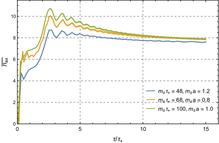
Figure 2: Axion production efficiency $\bar{n}_{\mathrm{ax}}$ for fixed $N=3,n=0$ and several $m_{r}\operatorname{a_{x}}$, $m_{r}\tau_{*}$ values. After complex early dynamics, there is a slow decay superposed with oscillations at a fequency of $\omega=2m_{a}$.

First consider $\tau/\tau_{*}$. We can make this quantity large by simply running our evolution for a long time. The longer we run, the larger $m_{a}$ becomes; information therefore propagates more slowly, and the requirement $\tau/\operatorname{a_{x}}<N_{x}/2$ need not be strictly enforced. But at the same time, the ratio $m_{a}/m_{r}$ increases. When this ratio reaches $1/2$, a process in which two angular excitations merge into a radial excitation, which is unphysical, becomes efficient, which can deplete the generated axion number, changing our results. Therefore we are obliged to terminate our evolution while $m_{a}<0.4m_{r}$ to avoid this. However, we find that, after complex early dynamics, $\bar{n}_{\mathrm{ax}}$ rather rapidly approaches its late-time behavior. The worst case occurs when the physical mass is fixed; the time evolution of $\bar{n}_{\mathrm{ax}}$ for a range of other lattice parameters in the case of $n=0$, $N=3$ is shown in Figure 2. After complex and interesting early dynamics, the $\bar{n}_{\mathrm{ax}}$ value settles towards a large-value asymptote, plus oscillations and an inverse-power tail. The oscillations represent some coherence in the fluctuations about $\theta_{\mathrm{a}}=0$ and have a frequency of $2m_{a}$; we eliminate them by always evaluating $\bar{n}_{\mathrm{ax}}$ at two times separated by $\pi/2m_{a}$ and averaging. This leaves a power-law decay towards the asymptotic value. The difference from the asymptotic value represents finite-angle effects and decays as $\sim\sum_{a\neq 1}\langle\Phi_{a}^{2}\rangle\propto(\tau_{*}/\tau)^{3+n/2}$. This functional form gives a good fit to the late-time behavior and we use it to extrapolate $(\tau/\tau_{*})\to\infty$ over the range $(\tau/\tau_{*})\in[10,15]$ for $n=0$ and $(\tau/\tau_{*})\in[2.4,2.8]$ for $n=7$. We do not perform this fitting procedure for $N=3$ and $n=7$ and instead just average two evaluations at $(\tau/\tau_{*})=2.8$ and $\pi/2m_{a}$ later, becasue the output of simulations was initially not set up for the extrapolation procedure. This does not significantly influence results though, because for $n=7$ the inverse power tail decays very rapidly. We verify on $N=4$ and $N=5$ that this method agrees with the extrapolation results to within 1%, where both methods are applicable on the more verbose output of those simulations.

	$40$	$50$	$85$	$100$
$0.8$	$7.12\pm 0.03$	$7.37\pm 0.03$	$7.72\pm 0.04$	$-$
$1.0$	$7.44\pm 0.04$	$7.69\pm 0.07$	$7.87\pm 0.09$	$7.76\pm 0.05$
$1.2$	$7.59\pm 0.03$	$7.68\pm 0.02$	$-$	$7.85\pm 0.04$

Table 1: Extracted values for $\bar{n}_{\mathrm{ax}}$ for $N=3$, $n=0$ and several other parameter values.

	$230$	$270$	$320$	$360$
$0.8$	$-$	$-$	$10.58\pm 0.18$	$10.86\pm 0.27$
$1.0$	$-$	$10.69\pm 0.26$	$10.81\pm 0.15$	$10.75\pm 0.17$
$1.2$	$10.45\pm 0.20$	$10.68\pm 0.31$	$10.97\pm 0.18$	$10.74\pm 0.20$

Table 2: Extracted $\bar{n}_{\mathrm{ax}}$ values for $N=3$ fields with $n=7$ (rapidly increasing explicit symmetry breaking) for several other parameter values.

The resulting $\bar{n}_{\mathrm{ax}}$ is displayed for $N=3$ field components and $n=0$ (fixed physical angular mass) for several combinations of $(m_{r}\tau_{*},m_{r}\operatorname{a_{x}})$ in Table 1, and for the $n=7$ case (rapidly increasing angular mass) in Table 2. We need to perform an extrapolation of this data, and similar data for other $N,n$ values, to the $m_{r}\tau_{*}\to\infty$ and $m_{r}\operatorname{a_{x}}\to 0$ limits. To do so it is necessary to establish the expected functional forms for each parameter dependence. We expect that the most infrared wave number relevant to the problem should be $k\sim\tau_{*}^{-1}$, the coherence length of the field at the time when the axion mass becomes important. The most UV scale is $k\sim m_{r}$, beyond which the field is no longer constrained to lie on the vacuum manifold. Provided that $m_{r}\operatorname{a_{x}}\ll\pi$, our lattice should be able to resolve physics on this most UV scale with errors which scale as $(m_{r}\operatorname{a_{x}})^{2}$, since our nearest-neighbor equations of motion and quadratic time update receive corrections of this order. Therefore we will assume lattice-spacing effects of this functional form.

To determine the dependence on $(m_{r}\tau_{*})$, we need to determine which scales are actually important to the final axion number count. If only the scale $k\sim\tau_{*}^{-1}$ is relevant and in the absence of any topological objects, the only role of $m_{r}$ would be to keep the field on the vacuum manifold. Since finite $m_{r}$ does not do so perfectly, the field could move slightly off its manifold by an amount $\sim(k|\Phi|/m_{r})^{2}\sim(m_{r}\tau_{*})^{-2}$, and we would expect corrections of this order. However, the early-time dynamics of the fields should enter a scaling regime which, we expect, generates a spectrum of fluctuations with all $k$ up to $k\sim m_{r}$. Typically such scaling dynamics generates fluctuations with equal energy per logarithmic wave-number interval, $\varepsilon\propto\int dk/k$, which according to Eq. (5) means $n_{\mathrm{ax}}\propto\int dk/k^{2}$. Since $m_{r}$ acts as an artificial UV cutoff on this integration, we expect an $\mathcal{O}(1/m_{r}\tau_{*})$ sized artifact due to finite $m_{r}$. Therefore the extrapolation to the “stiff” $m_{r}\to\infty$ limit should involve an inverse-linear power of $m_{r}\tau_{*}$.

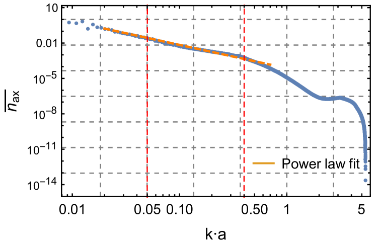
Figure 3: Log-log plot of the Fourier spectrum of the axion number $dn_{\mathrm{ax}}/dk$, for a four-component field with rapid turn-on of the explicit symmetry-breaking mass $n=7$, with $m_{r}\operatorname{a_{x}}=1.0$ and $m_{r}\tau_{*}=320$. Dashed red lines indicate the fitting region for a power law dependence. In this region, the axion number scales as $dn_{\mathrm{ax}}\propto dk/k^{2}$, indicating a linear sensitivity to the UV cutoff at the scale $m_{r}$. The behavior above $ka=0.5$ is modified by radial dynamics and the behavior above $ka=2$ is affected by the lattice regularization, but neither region contributes significantly.

We can check whether this is the case by computing the spectrum of axion fluctuations numerically from our final-time field configurations; we simply don’t do the $k$ integral in Eq. (5) but instead examine the Fourier spectrum of $n_{\mathrm{ax}}$. The result for the representative value $N=4,n=7$ is shown in Figure 3, which shows that the spectrum of excitations decays at large $k$ in the expected way. In particular, a power law $A\cdot x^{b}$ is fit to the region of the spectrum indicated, giving $b=-1.98(2)$ for Figure 3. As such, an $\mathcal{O}(1/m_{r}\tau_{*})$ fraction of the axion number should reside beyond the correctly-sampled scales and we therefore require $1/m_{r}\tau_{*}$ corrections in our extrapolation. Note that the presence of monopole topological defects could also lead to $1/m_{r}\tau_{*}$ corrections, since an $\mathcal{O}(1/m_{r})$ fraction of the monopole energy is contained in the core where the field unphysically departs from the vacuum manifold.

What about the lattice spacing? For $ka\ll 1$ the lattice treatment we use is accurate up to $(ka)^{2}$ corrections. This is largest for $k\sim m_{r}$, the shortest physically relevant scale. At this scale, lattice-spacing effects give rise to $(m_{r}a)^{2}$-suppressed corrections. But we have just seen that this scale only gives rise to an $\mathcal{O}(m_{r}\tau_{*})$-suppressed fraction of the axion number; therefore the expected size of lattice-spacing artifacts in the determined $\bar{n}_{\mathrm{ax}}$ value is of order $m_{r}a^{2}/\tau_{*}$. So the functional form we use to extrapolate to the small $a$ and large $m_{r}$ limits is

$$\bar{n}_{\mathrm{ax}}(m_{r}\tau_{*},m_{r}a)=(\bar{n}_{\mathrm{ax}})_{c}+A(m_{r}\tau_{*})^{-1}+Bm_{r}a^{2}/\tau_{*}$$ (13)

where $(\bar{n}_{\mathrm{ax}})_{c}$ is the desired continuum limit and $A,B$ are corrections. We find that this fitting form gives a good representation of our data, with $\chi^{2}/\mathrm{dof}$ of $2.114$ when $n=0$ and $0.404$ when $n=7$, respectively.

	$40$	$50$	$85$	$100$
$0.8$	$6.50\pm 0.03$	$6.78\pm 0.03$	$7.05\pm 0.08$	$-$
$1.0$	$6.74\pm 0.03$	$6.93\pm 0.02$	$7.19\pm 0.04$	$7.20\pm 0.05$
$1.2$	$6.84\pm 0.04$	$7.03\pm 0.03$	$-$	$7.26\pm 0.05$

Table 3: Extracted values for $\bar{n}_{\mathrm{ax}}$ for $N=4$, $n=0$ and several other parameter values.

	$230$	$270$	$320$	$360$
$0.8$	$-$	$-$	$11.27\pm 0.21$	$10.79\pm 0.29$
$1.0$	$10.72\pm 0.23$	$10.20\pm 0.40$	$10.39\pm 0.30$	$10.70\pm 0.4$
$1.2$	$10.28\pm 0.15$	$10.60\pm 0.22$	$10.50\pm 0.40$	$10.48\pm 0.25$

Table 4: Extracted $\bar{n}_{\mathrm{ax}}$ values for $N=4$ fields with $n=7$ (rapidly increasing explicit symmetry breaking) for several other parameter values.

	$40$	$50$	$85$	$100$
$0.8$	$6.06\pm 0.03$	$6.26\pm 0.05$	$6.57\pm 0.05$	$-$
$1.0$	$6.26\pm 0.03$	$6.42\pm 0.03$	$6.50\pm 0.03$	$6.69\pm 0.03$
$1.2$	$6.33\pm 0.03$	$6.46\pm 0.03$	$-$	$6.51\pm 0.04$

Table 5: Extracted values for $\bar{n}_{\mathrm{ax}}$ for $N=5$, $n=0$ and several other parameter values.

	$230$	$270$	$320$	$360$
$0.8$	$-$	$-$	$9.8\pm 0.5$	$8.7\pm 0.6$
$1.0$	$-$	$10.2\pm 0.4$	$11.0\pm 0.5$	$9.7\pm 0.4$
$1.2$	$10.06\pm 0.26$	$9.7\pm 0.4$	$10.5\pm 0.7$	$10.1\pm 0.4$

Table 6: Extracted $\bar{n}_{\mathrm{ax}}$ values for $N=5$ fields with $n=7$ (rapidly increasing explicit symmetry breaking) for several other parameter values.

We can repeat this extrapolation process now for N=4 and N=5. The results of this are shown in Tables 3, 4, 5, 6. For $N=4$ one finds a $\chi^{2}/\mathrm{dof}$ of $1.0853$ and $0.7354$ when $n=0$ or $n=7$. For $N=5$ one has $2.8566$ and $1.7671$ respectively.

4 Results

In the previous section we saw how to carry out extrapolations of finite-spacing, finite-$m_{r}$ data to the continuum and heavy-radial-field limits. We have done so for the cases of $N=3,4,5$ field components for each case of interest here – a fixed physical mass $n=0$ (that is, $m_{a,\mathrm{c}}^{2}=\tau^{2}/\tau_{*}^{4}$) and a rapidly growing mass $n=7$ or $m_{a,\mathrm{c}}^{2}=\tau^{9}/\tau_{*}^{11}$, analogous to how the axion mass increases cosmologically. Our central results are the axion production efficiencies for each of these cases, extrapolated to the late-time, fine-spacing, and large-radial-mass limits, which we present in Table 7. Each result in the table represents an extrapolation over 10 lattice spacing/$\tau_{*}$ combinations, each of which involved averaging at least $10$ independent lattice evolutions when $n=7$ and at least $6$ when $n=0$, except when $N=5$. Because $N=5$ is computationally more expensive, only half as many independent evolutions were performed, leading to increased statistical errors. In every case the continuum and large-$m_{r}$ extrapolations are very mild, with the final result always differing by less than 10% from the coarsest and smallest-$m_{r}$ lattice. The table represents the main results of this work.

$N$ $n$ $\bar{n}_{\mathrm{ax}}$ $\bar{n}_{\mathrm{misalign}}$ ratio 3 0 $8.10\pm 0.06$ 5.47 $1.48\pm 0.01$ 4 0 $7.58\pm 0.05$ 4.58 $1.65\pm 0.01$ 5 0 $6.78\pm 0.06$ 4.18 $1.62\pm 0.02$ 3 7 $11.52\pm 0.30$ 10.91 $1.05\pm 0.03$ 4 7 $10.66\pm 0.44$ 9.47 $1.12\pm 0.05$ 5 7 $10.05\pm 1.20$ 8.82 $1.14\pm 0.14$

Table 7: Dimensionless “axion” production efficiency (middle column), misalignment expectation, and their ratio (last column) for three values of $N$ the number of field components and two rates of angular-excitation mass-growth $n$.

5 Discussion and conclusions

As we see in the previous section, the production efficiency for “axions” is significantly higher than the misalignment estimate if the axion mass turns on gradually – for instance, if it remains fixed in physical units. In this case, the chaotic spatial distribution of the field leads to additional fluctuations. The discrepancy appears to get larger with more independent field components, but this turns out to be a weak effect; the total production declines with increasing $N$, at least for $N=3,4,5$.

However, when the axion mass turns on more abruptly – for instance, if $m_{a}^{2}\propto T^{-7}$, close to the physically relevant case for real axions – then our results are quite different. The production of angular fluctuations is quite close to the expectation based on the misalignment picture, and the expected trend – that the production is smaller for fields with more components – does emerge.

Naturally one cannot immediately take this result and conclude that the same is true of the $N=2$ field-component case, that is, actual axions. The presence of string topological defects, and their large role in the energy budget, is a significant difference from these higher-field-component models. Nevertheless, we have learned something important. When the explicit symmetry breaking turns on rapidly, that significantly changes the dynamics. The field rapidly becoming heavy makes gradient terms and long-range variation less important; the fields’ evolution become much more determined by the local field value and less by spatially varying structures. This could at least partly explain why the production efficiency for axions is also surprisingly small in the case where the axion mass grows as a high power of the conformal time.

References

- [1] Steven Weinberg. A New Light Boson? Phys.Rev.Lett., 40:223–226, 1978.
- [2] Frank Wilczek. Problem of Strong p and t Invariance in the Presence of Instantons. Phys.Rev.Lett., 40:279–282, 1978.
- [3] John Preskill, Mark B. Wise, and Frank Wilczek. Cosmology of the Invisible Axion. Phys. Lett., B120:127–132, 1983.
- [4] L. F. Abbott and P. Sikivie. A Cosmological Bound on the Invisible Axion. Phys. Lett., B120:133–136, 1983.
- [5] Michael Dine and Willy Fischler. The Not So Harmless Axion. Phys. Lett., B120:137–141, 1983.
- [6] Richard Lynn Davis. Cosmic Axions from Cosmic Strings. Phys. Lett., B180:225, 1986.
- [7] Luca Visinelli and Paolo Gondolo. Dark Matter Axions Revisited. Phys. Rev., D80:035024, 2009.
- [8] L. Visinelli and P. Gondolo. Axion cold dark matter in view of BICEP2 results. Phys. Rev. Lett., 113:011802, 2014.
- [9] Olivier Wantz and E. P. S. Shellard. The Topological susceptibility from grand canonical simulations in the interacting instanton liquid model: Chiral phase transition and axion mass. Nucl. Phys., B829:110–160, 2010.
- [10] Sz. Borsanyi et al. Calculation of the axion mass based on high-temperature lattice quantum chromodynamics. Nature, 539(7627):69–71, 2016.
- [11] Diego Harari and P. Sikivie. On the Evolution of Global Strings in the Early Universe. Phys. Lett., B195:361–365, 1987.
- [12] C. Hagmann, Sanghyeon Chang, and P. Sikivie. Axions from string decay. Nucl. Phys. Proc. Suppl., 72:81–86, 1999.
- [13] R. A. Battye and E. P. S. Shellard. Global string radiation. Nucl. Phys., B423:260–304, 1994.
- [14] R. A. Battye and E. P. S. Shellard. Axion string constraints. Phys. Rev. Lett., 73:2954–2957, 1994. [Erratum: Phys. Rev. Lett.76,2203(1996)].
- [15] Masahide Yamaguchi, M. Kawasaki, and Jun’ichi Yokoyama. Evolution of axionic strings and spectrum of axions radiated from them. Phys. Rev. Lett., 82:4578–4581, 1999.
- [16] Masahide Yamaguchi. Scaling property of the global string in the radiation dominated universe. Phys. Rev., D60:103511, 1999.
- [17] Takashi Hiramatsu, Masahiro Kawasaki, Toyokazu Sekiguchi, Masahide Yamaguchi, and Jun’ichi Yokoyama. Improved estimation of radiated axions from cosmological axionic strings. Phys.Rev., D83:123531, 2011.
- [18] Takashi Hiramatsu, Masahiro Kawasaki, Ken’ichi Saikawa, and Toyokazu Sekiguchi. Production of dark matter axions from collapse of string-wall systems. Phys.Rev., D85:105020, 2012.
- [19] Leesa Fleury and Guy D. Moore. Axion dark matter: strings and their cores. Journal of Cosmology and Astroparticle Physics, 2016(01):004, 2016.
- [20] Leesa M. Fleury and Guy D. Moore. Axion String Dynamics I: 2+1D. JCAP, 1605(05):005, 2016.
- [21] Vincent B.. Klaer and Guy D. Moore. The dark-matter axion mass. JCAP, 11:049, 2017.
- [22] Alejandro Vaquero, Javier Redondo, and Julia Stadler. Early seeds of axion miniclusters. JCAP, 04:012, 2019.
- [23] Malte Buschmann, Joshua W. Foster, and Benjamin R. Safdi. Early-Universe Simulations of the Cosmological Axion. Phys. Rev. Lett., 124(16):161103, 2020.
- [24] Marco Gorghetto, Edward Hardy, and Giovanni Villadoro. Axions from Strings: the Attractive Solution. JHEP, 07:151, 2018.
- [25] Marco Gorghetto, Edward Hardy, and Giovanni Villadoro. More Axions from Strings. SciPost Phys., 10:050, 2021.
- [26] T. W. B. Kibble. Topology of Cosmic Domains and Strings. J. Phys., A9:1387–1398, 1976.
- [27] Neil Turok. Global Texture as the Origin of Cosmic Structure. Phys. Rev. Lett., 63:2625, 1989.
- [28] Michael S. Turner. Windows on the Axion. Phys.Rept., 197:67–97, 1990.
- [29] Georg G. Raffelt. Astrophysical methods to constrain axions and other novel particle phenomena. Phys.Rept., 198:1–113, 1990.
- [30] Georg G. Raffelt. Particle physics from stars. Ann.Rev.Nucl.Part.Sci., 49:163–216, 1999.
- [31] Giovanni Grilli di Cortona, Edward Hardy, Javier Pardo Vega, and Giovanni Villadoro. The QCD axion, precisely. JHEP, 01:034, 2016.
- [32] Olivier Wantz and E.P.S. Shellard. Axion Cosmology Revisited. Phys.Rev., D82:123508, 2010.
- [33] Alexander Vilenkin. Cosmic strings. Phys. Rev. D, 24:2082–2089, 1981.
- [34] A. Vilenkin and A. E. Everett. Cosmic Strings and Domain Walls in Models with Goldstone and PseudoGoldstone Bosons. Phys. Rev. Lett., 48:1867–1870, 1982.
- [35] D. P. Bennett and S. H. Rhie. Cosmological evolution of global monopoles and the origin of large scale structure. Phys. Rev. Lett., 65:1709–1712, 1990.
- [36] John Preskill and Alexander Vilenkin. Decay of metastable topological defects. Phys. Rev., D47:2324–2342, 1993.
- [37] Vincent B. Klaer and Guy D. Moore. How to simulate global cosmic strings with large string tension. JCAP, 1710(10):043, 2017.