Stochastic orders and measures of skewness and dispersion based on expectiles

Abstract

Recently, expectile-based measures of skewness akin to well-known quantile-based skewness measures have been introduced, and it has been shown that these measures possess quite promising properties (Eberl and Klar, 2021, 2020). However, it remained unanswered whether they preserve the convex transformation order of van Zwet, which is sometimes seen as a basic requirement for a measure of skewness. It is one of the aims of the present work to answer this question in the affirmative. These measures of skewness are scaled using interexpectile distances. We introduce orders of variability based on these quantities and show that the so-called weak expectile dispersive order is equivalent to the dilation order. Further, we analyze the statistical properties of empirical interexpectile ranges in some detail.

Keywords: Expectile, skewness, stop-loss transform, dispersion order, dilation order, dispersive order, scale measure, asymptotic relativ efficiency.

1 Introduction

Over the last years, there was a steady increase in literature dealing with expectiles. These are measures of non-central location that have properties similar to quantiles. Therefore, expectiles can also be used as building blocks for measures of scale, skewness, etc. However, no such measure should be used without identification of the ordering it preserves.

Let us explain this in more detail. Since the seminal work of van Zwet (1964), Oja (1981), MacGillivray (1986), an axiomatic approach to measure statistical quantities is commonly accepted. It involves two main steps (Hürlimann, 2002):

• Define stochastic (partial) orders on sets of random variables or distribution functions that allow for comparisons of the given statistical quantity.

• Identify measures of the statistical quantity by considering functionals of distributions that preserve the partial order, and use only such measures in practical work.

Given a dispersion or variability ordering $\leq_{D}$, the general axiomatic approach requires that a scale measure $\delta$ satisfies

1. For $c,d\in\mathbb{R}$, $\delta(cX+d)=\lvert c\rvert\delta(X)$.

2. If $X\leq_{D}Y$, then $\delta(X)\leq\delta(Y)$.

Similarly, given a skewness order $\leq_{S}$, a skewness measure $\gamma$ should satisfy

1. For $c>0$ and $d\in\mathbb{R}$, $\gamma(cX+d)=\gamma(X)$.

2. The measure satisfies $\gamma(-X)=-\gamma(X)$.

3. If $X\leq_{S}Y$, then $\gamma(X)\leq\gamma(Y)$.

The generally accepted strongest dispersion and skewness orders are the dispersive order (Bickel and Lehmann, 1979) and the convex transformation order (van Zwet, 1964), respectively.

Research which treats expectile-based measures and related stochastic orderings includes Bellini (2012); Bellini et al. (2014, 2018a); Klar and Müller (2019); Eberl and Klar (2020, 2021); Arab et al. (2022). In particular, Eberl and Klar (2021, 2020) introduced expectile-based measures of skewness which possess quite promising properties and have close connections to other skewness functionals. However, it remained unanswered whether these measures preserve the convex transformation order. It is one of the aims of the present work to answer this question in the affirmative.

As part of these measures of skewness, interexpectile distances (also called interexpectile ranges) appear quite naturally; they have also been used in a finance context by Bellini et al. (2018b, 2020, 2021). We introduce orders of variability based on slightly more general quantities and show that the so-called weak expectile dispersive order is equivalent to the dilation order. Hence, interexpectile ranges preserve the dispersive ordering.

Up to now, statistical properties of empirical interexpectile ranges do not seem to have been investigated. We show that they are a good compromise between the standard deviation on the one hand and robust measures as the interquartile range on the other.

This paper is organized as follows. In Section 2, we recall the definitions of expectiles and some of their properties. Section 3 discusses expectile skewness. It is shown that expectile-based skewness measures are consistent with the convex transformation order. In Section 4, we introduce strong and weak expectile dispersive orders and show that the latter is equivalent to the dilation order. It follows that the interexpectile range preserves the dispersive order. These concepts are illustrated in Section 5, using the Lomax or Pareto type II distribution. Empirical interexpectile ranges are analyzed and compared with other scale measures in Section 6, using standardized asymptotic relative efficiencies.

2 Preliminaries

Throughout the paper, we assume that all mentioned random variables $X$ are non-degenerate, have a finite mean (denoted as $X\in L^{1}$), and are defined on a common probability space $(\Omega,\mathcal{A},P)$. Further, we assume that the supports of the underlying distributions are intervals and that these distributions have no atoms. Hence, the distribution function (cdf) $F_{X}$ of $X$ has a strictly increasing and continuous inverse on $(0,1)$.

Expectiles $e_{X}(\alpha)$ of a random variable $X\in L^{2}$ have been defined by Newey and Powell (1986) as the minimizers of an asymmetric quadratic loss:

$$e_{X}(\alpha)=\arg\min_{t\in\mathbb{R}}\left\{E\ell_{\alpha}(X-t)\right\}\text{,}$$ (1)

where

$$\ell_{\alpha}(x)=\begin{cases}\alpha x^{2},&\mbox{ if }x\geq 0,\\ (1-\alpha)x^{2},&\mbox{ if }x<0,\end{cases}$$

and $\alpha\in(0,1)$. For $X\in L^{1}$ (but $X\notin L^{2}$), equation (1) has to be modified (Newey and Powell, 1986) to

$$e_{X}(\alpha)=\arg\min_{t\in\mathbb{R}}\left\{E\left[\ell_{\alpha}(X-t)-\ell_{\alpha}(X)\right]\right\}.$$ (2)

The minimizer in (1) or (2) is always unique and is identified by the first order condition

$$\alpha E\left(X-e_{X}(\alpha)\right)_{+}=(1-\alpha)E\left(X-e_{X}(\alpha)\right)_{-}\text{,}$$ (3)

where $x_{+}=\max\{x,0\}$, $x_{-}=\max\{-x,0\}$. This is equivalent to characterizing expectiles via an identification function, which, for any $\alpha\in(0,1)$ is defined by

$$I_{\alpha}(x,y)=\alpha(y-x)\mathbbm{1}_{\{y\geq x\}}-(1-\alpha)(x-y)\mathbbm{1}_{\{y<x\}}$$

for $x,y\in\mathbb{R}$. The $\alpha$-expectile of a random variable $X\in L^{1}$ is then the unique solution of

$$EI_{\alpha}(t,X)=0,\quad t\in\mathbb{R}.$$

Similarly, the empirical $\alpha$-expectile $\hat{e}_{n}(\alpha)$ of a sample $X_{1},\ldots,X_{n}$ is defined as solution of

$$I_{\alpha}(t,\hat{F}_{n})=\frac{1}{n}\sum_{i=1}^{n}I_{\alpha}(t,X_{i})=0,\quad t\in\mathbb{R}.$$

Like quantiles, expectiles are measures of non-central location and have similar properties (see, e.g., Newey and Powell (1986) and Bellini et al. (2014)). Clearly, expectiles depend only on the distribution of the random variable $X$ and can be seen as statistical functionals defined on the set of distribution functions with finite mean on $\mathbb{R}$.

Throughout the paper, we make use of the following stochastic orders:

Definition 1.

1. $F_{X}$ precedes $F_{Y}$ in the usual stochastic order (denoted by $F_{X}\leq_{st}F_{Y}$) if $E\phi(X)\leq E\phi(Y)$ for all increasing functions $\phi$, for which both expectations exist.

2. $F_{X}$ precedes $F_{Y}$ in the convex order (denoted by $F_{X}\leq_{cx}F_{Y}$) if $E\phi(X)\leq E\phi(Y)$ for all convex functions $\phi$, for which both expectations exist.

3. $F_{X}$ precedes $F_{Y}$ in the convex transformation order (denoted by $F_{X}\leq_{c}F_{Y}$) if $F_{Y}^{-1}\circ F_{X}$ is convex.

4. $F_{X}$ precedes $F_{Y}$ in the expectile (location) order (denoted by $F_{X}\leq_{e}F_{Y}$) if

   $$e_{X}(\alpha)\leq e_{Y}(\alpha)\mbox{ for all }\alpha\in(0,1).$$

The first three orders are well-known (Shaked and Shantikumar, 2007; Müller and Stoyan, 2002); the expectile (location) order was introduced in Bellini et al. (2018a). Since the usual stochastic order $\leq_{st}$ is equivalent to the pointwise ordering of the quantiles, the definition of the expectile ordering is quite natural, just replacing quantiles by expectiles.

As noted by Jones (1994), expectiles are the quantiles of a suitably transformed distribution. Indeed, the first order condition (3) can be written in the equivalent form

$$\alpha =\frac{E\left(X-t\right)_{-}}{E\left|X-t\right|}=\frac{\pi_{X}(t)-\mu+t}{2\pi_{X}(t)-\mu+t}=:\breve{F}_{X}(t),$$ (4)

where $\mu=EX$ and $\pi_{X}(t)=E(X-t)_{+}$ denotes the stop-loss transform of $X$. Hence, $\breve{F}_{X}(t)=e_{X}^{-1}(t)$, and the expectile order could also be defined by $\breve{F}_{X}(t)\geq\breve{F}_{Y}(t)$ for all $t$. The expectile order is weaker than the usual stochastic order, i.e. $X\leq_{st}Y$ implies $X\leq_{e}Y$ (Bellini, 2012).

3 Expectile skewness

In the following, we summarize some results which are important with respect to expectile-based quantification of skewness. Bellini et al. (2018a), Thm. 12 and Cor. 13, show the following equivalence.

Proposition 2.

Let $X,Y\in L^{1}$ with $EX=EY=\mu$, $m=\operatorname*{ess\,inf}(X),M=\operatorname*{ess\,sup}(X)$. Then the following conditions are equivalent:

1. $X\leq_{e}Y$.

2. $\pi_{X}(x)\geq\pi_{Y}(x)$, for each $x\in(m,\mu)$ and $\pi_{X}(x)\leq\pi_{Y}(x)$, for each $x\in(\mu,M)$.

3. $(X-\mu)_{-}\geq_{cx}(Y-\mu)_{-}$ and $(X-\mu)_{+}\leq_{cx}(Y-\mu)_{+}$.

Eberl and Klar (2021) introduced a family of scalar measures of skewness

$$\tilde{s}_{2}(\alpha)=\frac{e_{X}(1-\alpha)+e_{X}(\alpha)-2\mu}{e_{X}(1-\alpha)-e_{X}(\alpha)},\quad\alpha\in(0,1/2),$$

and called a distribution right-skewed (left-skewed) in the expectile sense if $\tilde{s}_{2}(\alpha)\geq(\leq)\,0$ for all $\alpha\in(0,1/2)$ and equality does not hold for each $\alpha\in(0,1/2)$. If equality holds for each $\alpha$, the distribution is symmetric. They also defined a normalized version $s_{2}(\alpha)=\tilde{s}_{2}(\alpha)/(1-2\alpha)$, and proved that $-1<s_{2}(\alpha)<1$, and both inequalities are sharp for any $\alpha\in(0,1/2)$.

Moreover, Eberl and Klar (2021) introduced a function

$$S_{X}(t)=\frac{\pi_{X}(\mu+t)-\pi_{X}(\mu-t)}{t}+1=\frac{1}{t}\int_{\mu-t}^{\mu+t}F_{X}(z)dz-1,\quad t>0,$$

which has been shown to be strongly related to $s_{2}$: it holds that $s_{2}(\alpha)\geq 0$ for $\alpha\in(0,1/2)$ if and only if $S_{X}(t)\geq 0$ for each $t>0$ (Eberl and Klar, 2021). Based on $S_{X}$, the following two skewness orders have been defined, which are both weaker than van Zwet’s skewness order $\leq_{c}$ (Eberl and Klar, 2021).

Definition 3.

1. Let $\tilde{S}_{X}(t)=S_{X}(td_{X})$, where $d_{X}=E\lvert X-EX\rvert$ denotes the mean absolute deviation from the mean (MAD). Then, we write $F_{X}\leq_{sf}F_{Y}$ if $\tilde{S}_{X}(t)\leq\tilde{S}_{Y}(t)\,\forall\,t>0$.

2. $F_{Y}$ is more skew with respect to mean and MAD than $F_{X}$ ($F_{X}<_{\mu}^{d}F_{Y}$), if $F_{X}(d_{X}x+EX)$ and $F_{Y}(d_{Y}x+EY)$ cross each other exactly once on each side of $x=0$, with $F_{X}(EX)\leq F_{Y}(EY)$.

Arab et al. (2022) introduced a skewness order as follows.

Definition 4.

Let $X,Y\in L^{1}$, and define $\tilde{X}=(X-EX)/E\lvert X-EX\rvert,\tilde{Y}=(Y-EY)/E\lvert Y-EY\rvert$, with cdf’s $F_{\tilde{X}}$ and $F_{\tilde{Y}}$. $X$ is smaller than $Y$ in the $s$-order, denoted by $F_{X}\leq_{s}F_{Y}$, if

$$\int_{-\infty}^{x}F_{\tilde{X}}(t)dt \geq\int_{-\infty}^{x}F_{\tilde{Y}}(t)dt,\quad\forall x\leq 0,$$

and

$$\int_{x}^{\infty}\bar{F}_{\tilde{X}}(t)dt \leq\int_{x}^{\infty}\bar{F}_{\tilde{Y}}(t)dt,\quad\forall x\geq 0,$$

where $\bar{F}=1-F$ denotes the survival function.

Using well-known conditions for the convex order (see, e.g., (3.A.7) and (3.A.8) in Shaked and Shantikumar (2007)), $X\leq_{s}Y$ holds if $\tilde{X}_{-}\geq_{cx}\tilde{Y}_{-}$ and $\tilde{X}_{+}\leq_{cx}\tilde{Y}_{+}$. A comparison with Prop. 2c) yields that

$$X\leq_{s}Y\quad\Leftrightarrow\quad\tilde{X}\leq_{e}\tilde{Y}$$ (5)

With regard to the standardized variables, (5) establishes that larger expectiles correspond to a more skewed distribution. The equivalence in (5) was derived in Arab et al. (2022), Thm. 14, using a different argument.

Definition 4 entails $\int_{-x}^{x}(F_{\tilde{X}}(t)-F_{\tilde{Y}}(t))dt\leq 0$ for all $x>0$. However, this is equivalent to $\tilde{S}_{X}(x)\leq\tilde{S}_{Y}(x)$ for all $x>0$. Hence, $\leq_{sf}$, the skewness order defined by $\tilde{S}_{X}$, is weaker than the $\leq_{s}$-order. On the other hand, the proof of Thm. 13(2.) in Arab et al. (2022) shows that $\leq_{s}$ is weaker than the order $\leq_{\mu}^{d}$. Taking into account Thm. 3 in Eberl and Klar (2021), we obtain the following chain of implications:

$$X\leq_{c}Y\;\Rightarrow\;X\leq_{\mu}^{d}Y\;\Rightarrow\;X\leq_{s}Y\;\Rightarrow\;X\leq_{sf}Y.$$ (6)

The following theorem is the main result in this section, showing that the expectile-based skewness measure $s_{2}$ (and, hence, $\tilde{s}_{2}$) preserves van Zwet’s skewness order.

Theorem 5.

Let $X,Y\in L^{1}$. Then, $s_{2}$ is consistent with $\leq_{c}$, i.e. $X\leq_{c}Y$ implies $s_{2,X}(\alpha)\leq s_{2,Y}(\alpha)$ for each $\alpha\in(0,1/2)$.

Proof.

By (6) and (5), $X\leq_{c}Y$ implies $\tilde{X}\leq_{e}\tilde{Y}$, i.e. $e_{\tilde{X}}(\alpha)\leq e_{\tilde{Y}}(\alpha)$ for all $\alpha\in(0,1)$. A straightforward computation shows that $s_{2,\tilde{X}}(\alpha)\leq s_{2,\tilde{Y}}(\alpha)$ is equivalent to

$$e_{\tilde{Y}}(1-\alpha)e_{\tilde{X}}(\alpha)\leq e_{\tilde{X}}(1-\alpha)e_{\tilde{Y}}(\alpha),\quad\forall\alpha\in(0,1/2),$$

which, in turn, is equivalent to

$$e_{\tilde{Y}}(1-\alpha)\,\lvert e_{\tilde{X}}(\alpha)\rvert\geq e_{\tilde{X}}(1-\alpha)\,\lvert e_{\tilde{Y}}(\alpha)\rvert,\quad\forall\alpha\in(0,1/2).$$ (7)

Since, by assumption, $e_{\tilde{Y}}(1-\alpha)\geq e_{\tilde{X}}(1-\alpha)$ and $\lvert e_{\tilde{X}}(\alpha)\rvert\geq\lvert e_{\tilde{Y}}(\alpha)\rvert$ for $\alpha\in(0,1/2)$, inequality (7) holds. Since $s_{2}$ is invariant under location-scale transforms, $s_{2,X}(\alpha)\leq s_{2,Y}(\alpha)$ holds as well for all $\alpha\in(0,1/2)$. ∎

Remark 6.

If we write $X\leq_{s_{2}}Y$ if $s_{2,X}(\alpha)\leq s_{2,Y}(\alpha)$ for all $\alpha\in(0,1/2)$, the proof of Thm. 5 shows that $\leq_{s_{2}}$ is a weaker order of skewness than $\leq_{s}$. The question if $\leq_{s_{2}}$ implies $\leq_{sf}$ or vice versa is open. Another expectile based order, stronger than $\leq_{s_{2}}$, could be defined analogously to the quantile-based skewness order $\leq_{c}$, i.e. by

$$\frac{e_{X}(w)-2e_{X}(v)+e_{X}(u)}{e_{X}(w)-e_{X}(u)} \leq\frac{e_{Y}(w)-2e_{Y}(v)+e_{Y}(u)}{e_{Y}(w)-e_{Y}(u)}$$ (8)

for all $0<u<v<w<1$; this order is equivalent to the convexity of $\breve{F}_{Y}^{-1}\circ\breve{F}_{X}$, where $\breve{F}_{X}$ is defined in (4) (cp. Eberl and Klar (2021) for the quantile case). However, the above results are not strong enough to show that this order is weaker than $\leq_{c}$.

For the suitability of $s_{2}$ as a skewness measure, including its empirical counterpart, we refer to Eberl and Klar (2021) and Eberl and Klar (2020). To gain an impression, consider a Bernoulli distribution with success probability $p$. Clearly, for $p=1/2$, any skewness measure should be zero. For decreasing $p$, the distribution becomes more and more skewed to the right (note that the center decreases to 0), and a skewness measure should converge to its maximal possible value. Similarly, it should converge to its minimal possible value for $p\to 1$. For the expectile skewness, we obtain $s_{2}(\alpha)=1-2p$, independent of $\alpha$. The moment skewness is $(1-2p)/(p(1-p))$; quantile-based skewness measures are not uniquely defined for discrete distributions.

4 Expectile dispersive order and related measures

Additionally to the stochastic orders in Section 2, we need the following dispersion or variability orders.

Definition 7.

1. $F_{X}$ precedes $F_{Y}$ in the dispersive order (written $F_{X}\leq_{disp}F_{Y}$) if

   $$F_{X}^{-1}(v)-F_{X}^{-1}(u)\leq F_{Y}^{-1}(v)-F_{Y}^{-1}(u)\quad\forall\ 0<u<v<1.$$ (9)

2. $F_{X}$ precedes $F_{Y}$ in the weak dispersive order (written $F_{X}\leq_{w-disp}F_{Y}$) if (9) is fulfilled for all $0<u\leq 1/2\leq v<1$.

3. $F_{X}$ precedes $F_{Y}$ in the expectile dispersive order (written $F_{X}\leq_{e-disp}F_{Y}$) if

   $$e_{X}(v)-e_{X}(u)\leq e_{Y}(v)-e_{Y}(u)\quad\forall\ 0<u<v<1.$$ (10)

4. $F_{X}$ precedes $F_{Y}$ in the weak expectile dispersive order (written $F_{X}\leq_{we-disp}F_{Y}$) if (10) is fulfilled for all $0<u\leq 1/2\leq v<1$.

5. $F_{X}$ precedes $F_{Y}$ in the dilation order (written $F_{X}\leq_{dil}F_{Y}$) if

   $$X-EX\leq_{cx}Y-EY.$$ (11)

Remark 8.

The first ordering in Def. 7 is well-known (see, e.g., Bickel and Lehmann (1979), Oja (1981), Shaked (1982), Shaked and Shantikumar (2007)). The defining condition of the weak dispersive order, which is obviously weaker than the dispersive order, can be equivalently written as

$$F_{Y}^{-1}(u)-F_{X}^{-1}(u) \leq(\geq)\,F_{Y}^{-1}(1/2)-F_{X}^{-1}(1/2)\quad\text{for }u\leq(\geq)1/2.$$ (12)

This ordering was used in Bickel and Lehmann (1976) for symmetric distribution; for arbitrary distributions, it was introduced in MacGillivray (1986), Def. 2.6, and denoted by $\leq_{1}^{m}$. In introducing strong and weak expectile dispersive orders, we mimic these definitions. The following results show that the weak ordering defined in such a way has appealing theoretical properties; further, it corresponds to the expectile-based scale measures treated in Sec. 6. The expectile equivalent of the (strong) dispersive order from Def. 7(i) is shortly discussed in Example 12 and Remark 13.

We remark that Bellini et al. (2021) have introduced the following expectile based variability order which is even weaker than the weak expectile dispersive order:

$$X\leq_{\Delta-ex}Y,\quad\text{if }e_{X}(1-\alpha)-e_{X}(\alpha)\leq e_{Y}(1-\alpha)-e_{Y}(\alpha)\;\forall\ \alpha\in(0,1/2).$$

This order can be seen as a dispersion counterpart to the skewness order $\leq_{s_{2}}$ in Remark 6. The dilation order in Def. 7(v) is less well-known compared to the dispersive order, see Belzunce et al. (1997) or Fagiuoli et al. (1999). However, many of its properties follow from properties of the convex order.

Our main result in this section shows that the weak expectile dispersive order and the dilation order coincide. The proof uses the idea in the proof of Thm. 14 in Arab et al. (2022).

Theorem 9.

Let $X,Y\in L^{1}$ with strictly increasing cdf’s $F_{X}$ and $F_{Y}$ which are continuous on their supports. Then, $F_{X}\leq_{we-disp}F_{Y}$ if, and only if, $F_{X}\leq_{dil}F_{Y}$.

Proof.

Define $\tilde{X}=X-EX,\tilde{Y}=Y-EY$. Then, $X\leq_{dil}Y$ is equivalent to $\tilde{X}\leq_{cx}\tilde{Y}$, and therefore to $\pi_{\tilde{X}}(t)\leq\pi_{\tilde{Y}}(t)\,\forall t$. By continuity of $\pi_{\tilde{X}}$ and $\pi_{\tilde{Y}}$, this is equivalent to $\pi_{\tilde{X}}(t)/\lvert t\rvert\leq\pi_{\tilde{Y}}(t)/\lvert t\rvert\,\forall t\neq 0$, and hence to

$$\frac{\pi_{\tilde{X}}(t)}{t}\geq\frac{\pi_{\tilde{Y}}(t)}{t}\;\forall t<0\quad\text{and}\quad\frac{\pi_{\tilde{X}}(t)}{t}\leq\frac{\pi_{\tilde{Y}}(t)}{t}\;\forall t>0.$$ (13)

Note that, using the properties of the stop-loss transform (Müller and Stoyan, 2002, Thm. 1.5.10), $\pi_{\tilde{X}}(t)/t\leq-1$ for $t<0$, and $\pi_{\tilde{X}}(t)/t\geq 0$ for $t>0$. Now, applying to both sides of the inequalities the transformation $h(x)=(x+1)/(2x+1),x\neq-1/2$, which is decreasing for $x<-1/2$ as well as for $x>-1/2$, shows that (13) is equivalent to

$$\breve{F}_{\tilde{X}}(t)\leq\breve{F}_{\tilde{Y}}(t)\;\forall t<0\quad\text{and}\quad\breve{F}_{\tilde{X}}(t)\geq\breve{F}_{\tilde{Y}}(t)\;\forall t>0,$$ (14)

where $\breve{F}_{X}$ is the expectile cdf defined in (4). In turn, (14) is equivalent to

$$e_{\tilde{X}}(p)\geq e_{\tilde{Y}}(p)\;\forall p<1/2\quad\text{and}\quad e_{\tilde{X}}(p)\leq e_{\tilde{Y}}(p)\;\forall p>1/2.$$

This means that $e_{X}(p)-EX\geq e_{Y}(p)-EY\,\forall p<0\quad\text{and}\quad e_{X}(p)-EX\leq e_{Y}(p)-EY\,\forall p>0$, which is equivalent to $X\leq_{we-disp}Y$ (cp. the representation of the weak dispersive order in (12)). ∎

Remark 10.

Bellini (2012), Thm. 3(b) already proved that $X\leq_{cx}Y$ implies $e_{X}(\alpha)\geq e_{Y}(\alpha)$ for each $\alpha\leq 1/2$ and $e_{X}(\alpha)\leq e_{Y}(\alpha)$ for each $\alpha\geq 1/2$. From this, the implication $F_{X}\leq_{dil}F_{Y}\,\Rightarrow\,F_{X}\leq_{we-disp}F_{Y}$ follows, see also Bellini et al. (2018b). However, Thm. 9 also yields the reverse direction. Moreover, its proof is rather elementary, whereas Bellini (2012) employed techniques from monotone comparative statics.

Since, for random variables with finite mean, the dispersive order implies the dilation order (Shaked and Shantikumar (2007), Thm. 3.B.16), the next result is a direct consequence of Thm. 9.

Corollary 11.

Let $F_{X}$ and $F_{Y}$ be strictly increasing and continuous on their supports with finite expectations. Then, $X\leq_{disp}Y$ implies $X\leq_{we-disp}Y$.

In general, the (strong) expectile dispersive order in Def. 7(iii) is rather difficult to handle. However, the following example shows that this order does not imply the dispersive order (see also Remark 13c)).

It is an open question if the reverse direction holds, i.e. if the dispersive order implies the expectile dispersive order.

Example 12.

Let $p_{X},p_{Y}\in(0,1)$, $p_{X}\neq p_{Y}$ and $0<a_{X}<a_{Y}$. Furthermore, let $\tilde{X}\sim\mathrm{Bin}(1,p_{X}),\tilde{Y}\sim\mathrm{Bin}(1,p_{Y})$ and $X=a_{X}\cdot\tilde{X}$ and $Y=a_{Y}\cdot\tilde{Y}$. It follows directly that $X$ and $Y$ are not comparable with respect to $\leq_{disp}$ since $\mathrm{range}(F_{X})\subseteq\mathrm{range}(F_{Y})$ is a necessary condition for $X\leq_{disp}Y$ (Müller and Stoyan, 2002, Thm. 1.7.3). Further, a simple calculation yields $\pi_{X}(t)=p_{X}(a_{X}-t)$ for $t\in[0,a_{X}]$. It follows that

$$\breve{F}_{X}(t)=\frac{t(1-p_{X})}{p_{X}a_{X}+t(1-2p_{X})}\quad\text{and}\quad e_{X}(\alpha)=\frac{\alpha p_{X}a_{X}}{(1-\alpha)+p_{X}(2\alpha-1)}$$

for $t\in[0,a_{X}]$ and $\alpha\in(0,1)$ with analogous results for $Y$. Overall,

$$(e_{Y}\circ\breve{F}_{X})(t)=\frac{p_{Y}(1-p_{X})a_{Y}t}{p_{X}(1-p_{Y})a_{X}+t(p_{Y}-p_{X})}$$

for $t\in[0,a_{X}]$. Since $X\leq_{disp}Y$ is equivalent to $(F_{Y}^{-1}\circ F_{X})^{\prime}\geq 1$ (see, e.g., Oja, 1981, p. 157), $X\leq_{e-disp}Y$ is equivalent to $(e_{Y}\circ\breve{F}_{X})^{\prime}\geq 1$. Because of $\lim_{p_{X}\to p_{Y}}(e_{Y}\circ\breve{F}_{X})(t)=\frac{a_{Y}}{a_{X}}t$ for all $t\in[0,a_{X}]$, $X\leq_{e-disp}Y$ holds if the difference between $p_{X}$ and $p_{Y}$ is sufficiently small.

Since the involved distributions are discrete, this example does not fit in the general setting of this work. However, the statement of this example remains valid if the distributions of both $X$ and $Y$ are sufficiently closely approximated by continuous distributions (e.g. by linear interpolation). Overall, it is proved that $X\leq_{e-disp}Y\not\Rightarrow X\leq_{disp}Y$ in general.

5 Dispersion orders for the Lomax distribution

To illustrate the various concepts, we consider the Lomax or Pareto type II distribution having density, distribution and quantile function

$$f(t) =f(t;\alpha,\lambda)\ =\ \frac{\alpha}{\lambda}\left(1+\frac{t}{\lambda}\right)^{-(\alpha+1)},\quad t\geq 0,$$

$$F(t) =F(t;\alpha,\lambda)\ =\ 1-\left(1+t/\lambda\right)^{-\alpha},\quad t\geq 0,$$

$$q(p) =q(p;\alpha,\lambda)\ =\ \lambda\left((1-p)^{-1/\alpha}-1\right),\quad 0<p<1,$$

where $\alpha$ and $\lambda$ are positive parameters. Accordingly, the stop-loss transform is given by

$$\pi(t) =\frac{\lambda}{\alpha-1}\left(1+\frac{t}{\lambda}\right)^{1-\alpha},\quad t\geq 0,$$

and the expectile cdf $\breve{F}$ can explicitly computed by (4). Further, if $X\sim F(\cdot;\alpha,\lambda)$,

$$EX=\frac{\lambda}{\alpha-1}\;(\alpha>1), \quad Var(X)=\frac{\lambda^{2}\alpha}{(\alpha-1)^{2}(\alpha-2)}\;(\alpha>2).$$

In the following, assume $X\sim F(t;\alpha_{1},\lambda_{1})$ and $Y\sim F(t;\alpha_{2},\lambda_{2})$.

5.1 Dispersive order

If $X$ and $Y$ have densities $f_{X}$ and $f_{Y}$, then $X\leq_{disp}Y$ if, and only if,

$$f_{Y}\left(F^{-1}_{Y}(p)\right) \leq f_{X}\left(F^{-1}_{X}(p)\right)\quad\forall p\in(0,1)$$

(Shaked and Shantikumar, 2007, (3.B.119)). Applied to the Lomax distribution, $X\leq_{disp}Y$ iff

$$\frac{\alpha_{2}}{\lambda_{2}}(1-p)^{1/\alpha_{2}} \leq\frac{\alpha_{1}}{\lambda_{1}}(1-p)^{1/\alpha_{1}},\quad 0<p<1.$$ (15)

For $p$ converging to 0, (15) is fulfilled if

$$\frac{\lambda_{1}}{\alpha_{1}}\leq\frac{\lambda_{2}}{\alpha_{2}}.$$ (16)

Looking at $p\to 1$ shows that

$$\alpha_{1}\geq\alpha_{2}$$ (17)

is a second necessary condition for $X\leq_{disp}Y$. However, (16) and (17) are also sufficient: Taking the reciprocal of (15) shows that the inequality is equivalent to

$$\frac{1}{\alpha_{1}}q(p;\alpha_{1},\lambda_{1})+\frac{\lambda_{1}}{\alpha_{1}}\;\leq\;\frac{1}{\alpha_{2}}q(p;\alpha_{2},\lambda_{2})+\frac{\lambda_{2}}{\alpha_{2}}.$$ (18)

Now, (16) and (17) are necessary and sufficient for $X\leq_{st}Y$ (Bellini et al., 2018a). Hence, $q(p;\alpha_{1},\lambda_{1})\leq q(p;\alpha_{2},\lambda_{2})$ for all $p$, and (18) holds under (16) and (17). Overall, we have

$$X\leq_{st}Y\text{ as well as }X\leq_{disp}Y \;\text{ iff \; (\ref{cond-disp1}) and (\ref{cond-disp2}) hold}.$$

5.2 Weak expectile dispersive order

Here, we have to assume $\alpha_{1},\alpha_{2}>1$ for the expected values to exist. Define $H(p)=\frac{1}{1-p}\int_{p}^{1}F^{-1}(u)du$. Fagiuoli et al. (1999) showed that $X\leq_{dil}Y$ if, and only if,

$$H_{X}(p)-H_{X}(0) \leq H_{Y}(p)-H_{Y}(0),\quad 0<p<1.$$ (19)

For the Lomax distribution, $H(p)=(\alpha q(p)+\lambda)/(\alpha-1)$ and $H(0)=\lambda/(\alpha-1)$. Hence, (19) holds iff

$$\frac{\alpha_{1}\,q(p;\alpha_{1},\lambda_{1})}{\alpha_{1}-1} \leq\frac{\alpha_{2}\,q(p;\alpha_{2},\lambda_{2})}{\alpha_{2}-1},\quad 0<p<1.$$ (20)

A discussion of the behavior of $q(p)$ for $p\to 1$ shows that (17) is necessary for (20). Further, a second order Taylor expansion around $p=0$ yields $q(p)=\lambda p/\alpha+O(p^{2})$. Therefore, (20) can only be satisfied if

$$\frac{\lambda_{1}}{\alpha_{1}-1}\leq\frac{\lambda_{2}}{\alpha_{2}-1}.$$ (21)

Thus, (17) and (21) are necessary for $X\leq_{dil}Y$. We now show that they are also sufficient. Since $cq_{X}(p)=q_{cX}(p)$, and $\lambda$ is a scale parameter, (20) is equivalent to

$$q\left(p;\alpha_{1},\frac{\alpha_{1}\lambda_{1}}{\alpha_{1}-1}\right) \leq q\left(p;\alpha_{2},\frac{\alpha_{2}\lambda_{2}}{\alpha_{2}-1}\right),\quad 0<p<1.$$

This, in turn, is equivalent to

$$\bar{F}(p;\alpha_{1},\tilde{\lambda}_{1}) \leq\bar{F}(p;\alpha_{2},\tilde{\lambda}_{2}),\quad 0<p<1,$$ (22)

where $\tilde{\lambda}_{i}=\alpha_{i}\lambda_{i}/(\alpha_{i}-1),i=1,2.$ The above results about the usual stochastic order yield that (22) is satisfied iff $\alpha_{1}\geq\alpha_{2}$ and $\tilde{\lambda}_{1}/\alpha_{1}\leq\tilde{\lambda}_{2}/\alpha_{2}$, which coincide with (17) and (21).

Bellini et al. (2018a) have shown that these two conditions are also necessary and sufficient for the so-called increasing convex order ($\leq_{icx}$). Hence, we have the following result:

$$X\leq_{we-disp}Y\text{ as well as }X\leq_{icx}Y \;\text{ iff \; (\ref{cond-disp2}) and (\ref{cond-dil}) hold}.$$

Remark 13.

1. Assume $\alpha_{1}\geq\alpha_{2}>2$ and that (21) holds. Then, $\alpha_{1}/(\alpha_{1}-2)\leq\alpha_{2}/(\alpha_{2}-2)$, and $Var(X)\leq Var(Y)$ follows. Generally, the variance preserves the weak expectile dispersive order and therefore also the dilation order (see also the following section).

2. If $\alpha_{1}\geq\alpha_{2}$ and $\lambda_{1}/(\alpha_{1}-1)=\lambda_{2}/(\alpha_{2}-1)$, i.e. $EX=EY$, then $X\leq_{icx}Y$ corresponds to $X\leq_{cx}Y$. According to the last section, $X\leq_{we-disp}Y$ holds as well in this case.

   On the other hand, if $X$ and $Y$ are random variables from different Lomax distributions, but with equal means, they can never be ordered in expectile order (Bellini et al., 2018a). Since the dispersive order implies the stochastic order for distributions with the same finite left endpoint of their supports (Shaked and Shantikumar, 2007, Thm. 3.B.13), the expectile dispersive order then also implies the expectile (location) order (by applying the cited result to the expectile cdf’s $\breve{F}_{X}$ and $\breve{F}_{Y}$). Hence, $X$ and $Y$ can also not be ordered with respect to the expectile dispersive ordering. This example shows that $\leq_{we-disp}$ is strictly weaker than $\leq_{e-disp}$.

3. Let $\alpha_{1}=3,\lambda_{1}=\sqrt{3},\alpha_{2}=2,\lambda_{2}=1$. Since $\alpha_{1}>\alpha_{2}$ and $EX=\sqrt{3}/2<EY=1$, one has $X\leq_{we-disp}Y$. On the other hand, (16) is not satisfied. Hence, $X\leq_{disp}Y$ does not hold. In this example, $X$ also precedes $Y$ in the expectile location order (Bellini et al., 2018a, Thm. 23). The left panel of Figure 1 shows the interexpectile ranges of $X$ and $Y$; clearly, $e_{X}(1-p)-e_{X}(p)\leq e_{Y}(1-p)-e_{Y}(p)$ for $0<p<1$. The right panel shows a plot of $e_{Y}(\breve{F}_{X}(x))-x$, which is increasing in $x$. This indicates that also $X\leq_{e-disp}Y$ holds (Shaked and Shantikumar, 2007, (3.B.10)). Hence, similarly to Example 12, this shows that $X\leq_{e-disp}Y$ does not imply $X\leq_{disp}Y$ in general.

   

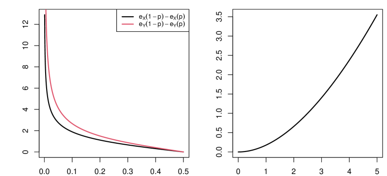
   Figure 1: Left panel: Interexpectile ranges of $X$ (in black) and $Y$ (in red) under Lomax distributions. Left panel: Plot of $e_{Y}(\breve{F}_{X}(x))-x$.

6 Interexpectile ranges and their empirical counterparts

It is clear that any functional of the form $E[\varphi(X-EX)]$, where $\varphi$ is a convex function, preserves the dilation order. Then, by Thm. 9, this also holds for the weak expectile dispersive order. Examples are the standard deviation $\sigma(F)=\{E(X-EX)^{2}\}^{1/2}$ and the mean absolute deviation around the mean $E\lvert X-EX\rvert$. In this section, however, we want to have a closer look on the interexpectile range (IER) $\mathcal{E}_{\alpha}=e_{X}(1-\alpha)-e_{X}(\alpha),\alpha\in(0,1/2)$. These scale measures obviously preserve the $\leq_{we-disp}$ ordering, and, hence, also the dilation order; they have already appeared as a scaling factor in the definition of $s_{2}$. Moreover, (implicit) interexpectile differences have been used to extract information about the risk-neutral distribution of a financial index by Bellini et al. (2018b, 2020).

Using the properties of expectiles (see, e.g., Bellini et al. 2014), $\mathcal{E}_{\alpha}$ obviously satisfies property D1. in the introduction. Hence, it is a measure of variability with respect to the dispersive order, the most fundamental variability ordering, but also with respect to the dilation order. The latter is an order with respect to the mean, whereas the first order is location-free. Further properties of the theoretical IER can be found in Bellini et al. (2018b), Prop. 3.1.

The results in Sec. 3 show that the MAD arises quite naturally when dealing with expectile-based skewness orders. Our next result bounds $\mathcal{E}_{\alpha}$ in terms of the MAD.

Theorem 14.

For $\alpha\in(0,1/2)$,

$$\frac{1-2\alpha}{1-\alpha}E\lvert X-\mu\rvert <\mathcal{E}_{\alpha}\,<\frac{1-2\alpha}{\alpha}E\lvert X-\mu\rvert.$$

In particular, $\frac{2}{3}E\lvert X-\mu\rvert<\mathcal{E}_{1/4}<2E\lvert X-\mu\rvert$.

Proof.

For any $\tau\in(0,1)\setminus\{1/2\}$, the first order condition (3) can be rewritten as

$$E(X-e_{X}(\tau))_{+} =\frac{1-\tau}{1-2\tau}(\mu-e_{X}(\tau)),$$ (23)

$$E(X-e_{X}(\tau))_{-} =\frac{\tau}{1-2\tau}(\mu-e_{X}(\tau)).$$ (24)

Since $E(X-t)_{+}$ is strictly decreasing and $E(X-t)_{-}$ is strictly increasing, and since $e_{X}(\alpha)<\mu<e_{X}(1-\alpha)$, we further obtain

$$E(X-e_{X}(1-\alpha))_{+} <E(X-\mu)_{+}<E(X-e_{X}(\alpha))_{+},$$ (25)

$$E(X-e_{X}(\alpha))_{-} <E(X-\mu)_{-}<E(X-e_{X}(1-\alpha))_{-}.$$ (26)

Adding the terms in (25) and (26), and using equations (23) and (24) then yields

$$\frac{\alpha}{1-2\alpha}\left(e_{X}(1-\alpha)-e_{X}(\alpha)\right) <E\lvert X-\mu\rvert\,<\frac{1-\alpha}{1-2\alpha}\left(e_{X}(1-\alpha)-e_{X}(\alpha)\right),$$

or

$$\frac{1-2\alpha}{1-\alpha}E\lvert X-\mu\rvert <e_{X}(1-\alpha)-e_{X}(\alpha)\,<\frac{1-2\alpha}{\alpha}E\lvert X-\mu\rvert.$$

∎

For any $\alpha\in(0,1/2)$, we define the population counterparts of $\mathcal{E}_{\alpha}$ by $\widehat{\mathcal{E}}_{\alpha,n}=\hat{e}_{n}(1-\alpha)-\hat{e}_{n}(\alpha)$. For empirical expectiles, a multivariate central limit theorem as well as strong consistency holds (see, e.g., Holzmann and Klar, 2016); from these results, a central limit theorem and strong consistency of $\widehat{\mathcal{E}}_{\alpha,n}$ can be derived. Using the notations $\eta(\tau_{1},\tau_{2})=E[I_{\tau_{1}}(e_{X}(\tau_{1}),X)I_{\tau_{2}}(e_{X}(\tau_{2}),X)]$ for $\tau_{1},\tau_{2}\in(0,1)$ and $a_{\alpha}=\alpha+(1-2\alpha)F(e_{X}(\alpha))$, the following holds true.

Theorem 15.

Let $F_{X}$ be a cdf with $E\lvert X\rvert<\infty$, and $\alpha\in(0,1/2)$.

1. If $EX^{2}<\infty$ and $F_{X}$ does not have a point mass at $e_{X}(\alpha)$ or $e_{X}(1-\alpha)$, then

   $$\sqrt{n}\left(\widehat{\mathcal{E}}_{\alpha,n}-\mathcal{E}_{\alpha}\right)\stackrel{{\scriptstyle\mathcal{D}}}{{\longrightarrow}}\mathcal{N}(0,\sigma^{2}_{\mathcal{E}}(\alpha)),$$

   where

   $$\sigma^{2}_{\mathcal{E}}(\alpha) =\,\frac{\eta(\alpha,\alpha)}{a_{\alpha}^{2}}-\frac{2\eta(\alpha,1-\alpha)}{a_{\alpha}\cdot a_{1-\alpha}}+\frac{\eta(1-\alpha,1-\alpha)}{a_{1-\alpha}^{2}}.$$

2. $\widehat{\mathcal{E}}_{\alpha,n}$ is a strongly consistent estimator of $\mathcal{E}_{\alpha}$, i.e.

   $$\widehat{\mathcal{E}}_{\alpha,n}\stackrel{{\scriptstyle a.s.}}{{\longrightarrow}}\mathcal{E}_{\alpha}.$$

A natural competitor to $\mathcal{E}_{\alpha}$ is the interquantile range (IQR) $\mathcal{Q}_{\alpha}=q_{X}(1-\alpha)-q_{X}(\alpha),\alpha\in(0,1/2)$, where $q_{X}(\alpha)$ denotes the $\alpha$-quantile of the distribution of $X$. By definition, the interquantile range preserves the dispersive order. However, it is not consistent with the dilation order, which may be seen as a disadvantage in specific applications (Bellini et al., 2020).

A general comparison result between the IQR and IER is not possible: $\mathcal{Q}_{\alpha}$ may be smaller than $\mathcal{E}_{\alpha}$ for some $\alpha$, and larger for other ones. However, such a comparison is possible for symmetric log-concave distributions such as the normal, logistic, uniform or Laplace distribution. This follows directly from Corollary 7 and the preceding results in Arab et al. (2022):

Proposition 16.

Let $F_{X}$ be a symmetric cdf with finite mean and log-concave density. Then,

$$\mathcal{E}_{\alpha} <\mathcal{Q}_{\alpha}\quad\text{for each }\alpha\in(0,1/2).$$

In the following, we compare the efficiency of the empirical IER as an estimator of the variability for specific distributions with other measures of dispersion, in particular with the IQR. Writing $\widehat{\mathcal{Q}}_{\alpha,n}=\hat{q}_{n}(1-\alpha)-\hat{q}_{n}(\alpha)$, where $\hat{q}_{n}(\alpha)$ is the sample quantile, one has

$$\sqrt{n}(\widehat{\mathcal{Q}}_{\alpha,n}-\mathcal{Q}_{\alpha})\stackrel{{\scriptstyle\mathcal{D}}}{{\longrightarrow}}\mathcal{N}\left(0,\sigma^{2}_{\mathcal{Q}}(\alpha)\right),$$

where

$$\sigma^{2}_{\mathcal{Q}}(\alpha)=\frac{\alpha(1-\alpha)}{f^{2}(q_{X}(1-\alpha))}-\frac{2\alpha^{2}}{f(q_{X}(\alpha))f(q_{X}(1-\alpha))}+\frac{\alpha(1-\alpha)}{f^{2}(q_{X}(\alpha))},$$

and $f$ denotes the density of $F_{X}$.

If $X\sim\mathcal{N}(\mu,\sigma^{2})$, we obtain $\sigma^{2}_{\mathcal{Q}}(\alpha)=2\alpha(1-2\alpha)/f^{2}(q_{X}(\alpha))$, and $\mathcal{Q}(\alpha)=2\sigma\Phi^{-1}(1-\alpha)$. Therefore,

$$\sqrt{n}\left(\frac{\widehat{\mathcal{Q}}_{\alpha,n}}{2\Phi^{-1}(1-\alpha)}-\sigma\right)\stackrel{{\scriptstyle\mathcal{D}}}{{\longrightarrow}}\mathcal{N}\left(0,\tau^{2}_{\mathcal{Q}}(\alpha)\sigma^{2}\right),$$

where

$$\tau^{2}_{\mathcal{Q}}(\alpha)=\frac{\alpha(1-2\alpha)}{2\left(\Phi^{-1}(1-\alpha)\right)^{2}\,\varphi^{2}\left(\Phi^{-1}(1-\alpha)\right)}.$$

On the other hand, the sample standard deviation $\widehat{\sigma}_{n}=(1/(n-1)\sum_{i=1}^{n}(X_{i}-\bar{X}_{n})^{2})^{1/2}$ has asymptotic variance $(\mu_{4}-\sigma^{4})/(4\sigma^{2})$, where $\mu_{4}=E(X-\mu)^{4}$, which simplifies to $\sigma^{2}/2$ under normality. Hence, the standardized asymptotic relative efficiency (ARE) is given by

$$sARE(\widehat{\mathcal{Q}}_{\alpha,n},\widehat{\sigma}_{n})=\frac{1/2}{\tau^{2}_{\mathcal{Q}}(\alpha)}.$$

We term $\tau^{2}_{\mathcal{Q}}(\alpha)$ the standardized asymptotic variance (standardized ASV). Proceeding in the same way with the IER leads to the corresponding quantity $\tau^{2}_{\mathcal{E}}(\alpha)=\sigma^{2}_{\mathcal{E}}(\alpha)/(2e_{X}(1-\alpha))^{2}$. Figure 2 shows the standardized ASV’s $\tau^{2}_{\mathcal{Q}}(\alpha)$ and $\tau^{2}_{\mathcal{E}}(\alpha)$ as functions of $\alpha$.

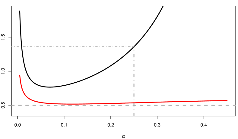
Figure 2: Standardized asymptotic variances $\tau^{2}_{\mathcal{Q}}(\alpha)$ (in black) and $\tau^{2}_{\mathcal{E}}(\alpha)$ (in red) under normality.

For the interquartile range, i.e. the choice $\alpha=1/4$, one obtains the well known result $sARE(\widehat{\mathcal{Q}}_{1/4,n},\widehat{\sigma}_{n})=0.368$; the standardized ARE takes the maximal value $0.652$ for $\alpha=0.0692$ (Fisher, 1920; David, 1998). Whereas the latter estimator is more efficient, an advantage of using more central quantiles such as quartiles is their greater stability.

Proceeding to the IER, Fig. 2 shows that the standardized ASV’s are generally smaller and quite stable over a large range of $\alpha$-values. For $\alpha=1/4$, we obtain $sARE(\widehat{\mathcal{E}}_{1/4,n},\widehat{\sigma}_{n})=0.934$; the standardized ARE takes the maximal value $0.967$ for $\alpha=0.118$. Hence, the IER is a quite efficient scale estimator under normality compared to the standard deviation.

To analyze the behaviour of the IER under distributions with longer tails than the normal, we consider in the following Student’s $t$-distribution with $\nu$ degrees of freedom, denoted by $t_{\nu}$, and having density function $c_{\nu}(1+x^{2}/\nu)^{-(\nu+1)/2},x\in\mathbb{R}$, for $\nu>0$, where $c_{\nu}=\Gamma((\nu+1)/2)/(\sqrt{\nu\pi}\Gamma(\nu/2))$.

Additionally to the dispersion measures used so far, we consider the MAD $d=E\lvert X-EX\rvert$, estimated by $\widehat{d}_{n}=1/n\sum_{i=1}^{n}\lvert X_{i}-\bar{X}_{n}\rvert$, and Gini’s mean difference $g=E\lvert X-Y\rvert$, where $Y$ is a independent copy of $X$. The usual estimator of $g$ is the sample mean difference $\widehat{g}_{n}=\frac{2}{n(n-1)}\sum_{i<j}\lvert X_{i}-X_{j}\rvert$. The asymptotic variance of $\widehat{d}_{n}$ is given by

$$ASV(\widehat{d}_{n}) =Var\left(\lvert X-\mu\lvert+(2F(\mu)-1)X\right)$$

(van der Vaart, 1998, Example 19.25), which simplifies to $ASV(\widehat{d}_{n})=\sigma^{2}-d^{2}$ for symmetric distributions. In this case, the ASV is the same as for the sample MAD around the median $1/n\sum_{i=1}^{n}\lvert X_{i}-q_{X}(1/2)\rvert$ (Gerstenberger and Vogel, 2015). An explicit expression for the ASV of $\widehat{g}_{n}$ under the $t$-distribution can be found in Gerstenberger and Vogel (2015), Table 3.

Similarly as above, given a scale measure $\delta$ and its estimator $\hat{\delta}$, we call the ratio $ASV(\hat{\delta})/\delta^{2}$ standardized asymptotic variance. Table 1 shows the standardized ASV of the different estimators for the $t$-distribution with various degrees of freedom.

	$\widehat{\sigma}$	$\widehat{\mathcal{E}}_{0.15}$	$\widehat{\mathcal{E}}_{0.25}$	$\widehat{\mathcal{E}}_{0.35}$	$\widehat{d}$	$\widehat{g}$	$\widehat{\mathcal{Q}}_{0.15}$	$\widehat{\mathcal{Q}}_{0.25}$	$\widehat{\mathcal{Q}}_{0.35}$
$t_{3}$	-	2.020	1.651	1.517	1.467	1.907	1.330	1.613	2.726
$t_{4}$	-	1.198	1.057	1.012	1.000	1.165	1.200	1.540	2.685
$t_{5}$	2.000	0.949	0.871	0.851	0.851	0.932	1.129	1.500	2.661
$t_{6}$	1.250	0.832	0.782	0.774	0.778	0.820	1.085	1.475	2.646
$t_{7}$	1.000	0.765	0.730	0.728	0.735	0.754	1.055	1.457	2.636
$t_{8}$	0.875	0.721	0.696	0.698	0.707	0.712	1.034	1.444	2.628
$t_{9}$	0.800	0.690	0.672	0.677	0.687	0.682	1.017	1.434	2.622
$t_{10}$	0.750	0.667	0.655	0.661	0.672	0.659	1.004	1.426	2.617
$t_{12}$	0.688	0.636	0.630	0.639	0.651	0.629	0.986	1.415	2.611
$t_{15}$	0.636	0.608	0.608	0.619	0.632	0.601	0.967	1.403	2.604
$t_{20}$	0.594	0.583	0.587	0.601	0.615	0.575	0.949	1.392	2.597
$t_{30}$	0.558	0.559	0.569	0.584	0.599	0.552	0.932	1.382	2.590
$t_{40}$	0.542	0.549	0.560	0.576	0.592	0.541	0.924	1.376	2.587
$t_{50}$	0.533	0.543	0.555	0.572	0.587	0.535	0.919	1.373	2.585
$t_{100}$	0.516	0.531	0.545	0.563	0.579	0.523	0.909	1.367	2.581

Table 1: Standardized ASV of different scale estimators for the $t_{\nu}$-distribution.

Concerning the comparison between the interquantile and interexpectile range, we observe a similar behavior as for the normal distribution. Whereas the standardized ASV’s vary strongly with $\alpha$ for the IQR, they are quite stable for the IER. To allow for a better comparison of the relative efficiencies, Table 2 shows the minimum of the standardized ASV’s in each line of Table 1, divided by the standardized ASV’s. Hence, for each distribution, the table shows the sARE with respect to the most efficient estimator. Whereas $\widehat{\mathcal{Q}}_{0.15}$ and $\widehat{d}$ are most efficient for $\nu=3$ and $\nu=4,5$, respectively, the IER gets in the lead for degrees of freedom between 6 and 10. For higher degrees of freedom, Gini’s mean difference and the standard deviation are most efficient.

	$\widehat{\sigma}$	$\widehat{\mathcal{E}}_{0.15}$	$\widehat{\mathcal{E}}_{0.25}$	$\widehat{\mathcal{E}}_{0.35}$	$\widehat{d}$	$\widehat{g}$	$\widehat{\mathcal{Q}}_{0.15}$	$\widehat{\mathcal{Q}}_{0.25}$	$\widehat{\mathcal{Q}}_{0.35}$
$t_{3}$	-	0.659	0.806	0.877	0.907	0.698	1.000	0.825	0.488
$t_{4}$	-	0.835	0.946	0.988	1.000	0.859	0.834	0.649	0.372
$t_{5}$	0.425	0.896	0.976	0.999	1.000	0.913	0.753	0.567	0.320
$t_{6}$	0.619	0.930	0.989	1.000	0.995	0.944	0.713	0.525	0.292
$t_{7}$	0.728	0.952	0.997	1.000	0.991	0.965	0.690	0.500	0.276
$t_{8}$	0.796	0.966	1.000	0.998	0.985	0.978	0.674	0.482	0.265
$t_{9}$	0.840	0.974	1.000	0.993	0.978	0.986	0.660	0.469	0.256
$t_{10}$	0.873	0.981	1.000	0.990	0.974	0.993	0.652	0.459	0.250
$t_{12}$	0.915	0.988	0.998	0.984	0.966	1.000	0.638	0.444	0.241
$t_{15}$	0.944	0.988	0.989	0.970	0.950	1.000	0.621	0.428	0.231
$t_{20}$	0.969	0.987	0.980	0.957	0.936	1.000	0.606	0.413	0.222
$t_{30}$	0.990	0.987	0.971	0.945	0.922	1.000	0.592	0.400	0.213
$t_{40}$	0.999	0.986	0.967	0.939	0.915	1.000	0.586	0.393	0.209
$t_{50}$	1.000	0.982	0.960	0.931	0.907	0.996	0.580	0.388	0.206
$t_{100}$	1.000	0.972	0.946	0.916	0.891	0.986	0.567	0.377	0.200

Table 2: sARE of different scale estimators with respect to the most efficient estimator for the $t_{\nu}$-distribution.

As a final example, we use the normal inverse Gaussian (NIG) distribution (Barndorff-Nielsen, 1997), which allows for skewed and heavy-tailed distributions; further, all moments exist and have simple explicit expressions. Table 3 shows the standardized ASV’s of the different estimators for the NIG distribution with shape parameters $\alpha$ and $\beta$. For $\beta=0$, the distribution is symmetric. The two remaining parameters are chosen such that $EX=0$ and $Var(X)=1$; hence, the third and fourth moment in columns 3-4 corresponds to the moment skewness and kurtosis. Note that, for $\beta=0$ and $\alpha\to\infty$, the distribution converges to the standard normal.

$\alpha$	$\beta$	$m_{3}$	$m_{4}$	$\widehat{\sigma}$	$\widehat{\mathcal{E}}_{0.25}$	$\widehat{d}$	$\widehat{g}$	$\widehat{\mathcal{Q}}_{0.25}$
10.0	0.0	0.00	3.03	0.507	0.540	0.575	0.517	1.364
10.0	8.0	0.67	3.82	0.706	0.654	0.679	0.620	1.009
10.0	9.0	1.42	6.52	1.381	1.017	1.016	0.938	0.713
2.0	0.0	0.00	3.75	0.688	0.642	0.662	0.640	1.433
2.0	1.0	1.00	5.67	1.167	0.882	0.881	0.848	0.990
2.0	1.5	2.57	15.73	3.684	1.979	1.891	1.735	0.655
1.0	0.0	0.00	6.00	1.250	0.910	0.884	0.947	1.602
1.0	0.5	2.00	13.67	3.167	1.654	1.564	1.531	1.020
1.0	0.8	6.67	85.41	21.102	7.112	6.607	5.379	0.877

Table 3: Standardized ASV of different scale estimators for the NIG-distribution.

From Table 3 we see that $\widehat{\mathcal{E}}_{0.25},\widehat{d}$ and $\widehat{g}$ have comparable standardized ASV’s. They are all quite efficient compared to $\widehat{\sigma}$ for distributions near to the normal. They are considerably more efficient than $\widehat{\sigma}$ for skewed and long-tailed distributions as the NIG distribution with $\alpha=1,\beta=0.5$, and compare well with the IQR in this case. All in all, these measures seem to be a reasonable compromise between the standard deviation on the one hand, and the interquartile range on the other.

Acknowledgments

We thank the two anonymous reviewers for their constructive and helpful comments. In particular, we thank one of the reviewers for pointing to the result stated as Prop. 16.

References

- Arab et al. (2022) Arab, I., Lando, T., Oliveira, P. E. (2022). Comparison of -quantiles and related skewness measures. Statistics and Probability Letters 183, 109339.
- Barndorff-Nielsen (1997) Barndorff-Nielsen, O. E. (1997). Normal inverse Gaussian distributions and stochastic volatility modelling. Scandinavian Journal of Statistics 24, 1-13.
- Bellini (2012) Bellini, F. (2012). Isotonicity results for generalized quantiles. Statistics and Probability Letters 82, 2017-2024
- Bellini et al. (2014) Bellini, F., Klar, B., Müller, A., Rosazza Gianin, E. (2014). Generalized quantiles as risk measures. Insurance: Mathematics and Economics 54, 41-48.
- Bellini et al. (2018a) Bellini, F., Klar, B., Müller, A. (2018a). Expectiles, Omega ratios and stochastic ordering. Methodology and Computing in Applied Probability 20, 855-873.
- Bellini et al. (2018b) Bellini, F. , Mercuri, L. and Rroji, E. (2018b), Implicit expectiles and measures of implied volatility. Quant. Finance 18, 1851-1864.
- Bellini et al. (2020) Bellini, F., Mercuri, L. and Rroji, E. (2020). On the dependence structure between S&P500, VIX and implicit interexpectile differences. Quant. Finance 20, 1839-1848.
- Bellini et al. (2021) Bellini, F., Fadina, T., Wang, R. and Wei, Y (2021). Parametric measures of variability induced by risk measures. Working paper, arXiv:2012.05219v2.
- Belzunce et al. (1997) Belzunce, F., Pellerey, F., Ruiz, J. M., Shaked, M. (1997). The dilation order, the dispersion order, and orderings of residual lives. Statistics & Probability Letters 33, 263-275.
- Bickel and Lehmann (1976) Bickel, P.J. and Lehmann, E.L. (1976). Descriptive statistics for nonparametric models III. Dispersion. Annals of Statistics 4, 1139-1158.
- Bickel and Lehmann (1979) Bickel, P.J. and Lehmann, E.L. (1979). Descriptive statistics for nonparametric models IV. Spread. In: J. Jureckova (Ed.), Contributions to Statistics, Academia, Prague (1979), 33-40.
- David (1998) David, H. A. (1998). Early sample measures of variability Statistical Science 13, 368-377.
- Eberl and Klar (2020) Eberl, A., Klar, B. (2020). Asymptotic distributions and performance of empirical skewness measures. Comput. Statist. Data Anal., 146, 106939.
- Eberl and Klar (2021) Eberl, A., Klar, B. (2021). Expectile based measures of skewness. Scandinavian Journal of Statistics. https://doi.org/10.1111/sjos.12518
- Fagiuoli et al. (1999) Fagiuoli, E., Pellerey, F., Shaked, M. (1999). A characterization of the dilation order and its applications. Statistical Papers 40, 393-406.
- Fisher (1920) Fisher, R. A. (1920). A mathematical examination of the methods of determining the accuracy of an observation by the mean error, and by the mean square error. Monthly Notices of the Royal Astronomical Society 80, 758-770.
- Gerstenberger and Vogel (2015) Gerstenberger, C., Vogel, D. (2015). On the efficiency of Gini’s mean difference. Statistical Methods & Applications, 24, 569-596.
- Holzmann and Klar (2016) Holzmann, H., Klar, B. (2016). Expectile asymptotics. Electronic Journal of Statistics 10, 2355-2371.
- Hürlimann (2002) Hürlimann, W. (2002). On risk and price: stochastic orderings and measures. Transactions 27th International Congress of Actuaries, Cancun.
- Jones (1994) Jones, M.C. (1994). Expectiles and M-quantiles are quantiles. Statistics and Probability Letters 20, 149-153.
- Klar and Müller (2019) Klar, B., Müller, A. (2019). On consistency of the Omega ratio with stochastic dominance rules. In: Innovations in Insurance, Risk-and Asset Management. World Scientific, 367-380.
- MacGillivray (1986) MacGillivray, H. L., 1986. Skewness and asymmetry: measures and orderings. The Annals of Statistics, 14, 994–1011.
- Müller (1996) Müller, A. (1996). Ordering of risks: A comparative study via stop-loss transforms. Insurance: Mathematics and Economics 17, 215-222.
- Müller and Stoyan (2002) Müller, A., Stoyan, D. (2002). Comparison methods for stochastic models and risks. John Wiley & Sons Ltd., Chichester.
- Newey and Powell (1986) Newey, K., Powell, J. (1986). Asymmetric least squares estimation and testing. Econometrica 55, 819-847.
- Oja (1981) Oja, H. (1981). On location, scale, skewness and kurtosis of univariate distributions. Scandinavian Journal of Statistics, 8, 154–168.
- Shaked (1982) Shaked, M. (1982). Dispersive ordering of distributions. Journal of Applied Probability 19, 310-320.