Asymmetry in earthquake interevent time intervals
Abstract
Here we focus on a basic statistical measure of earthquake catalogs that has not been studied before, the asymmetry of interevent time series (e.g., reflecting the tendency to have more aftershocks than spontaneous earthquakes). We define the asymmetry metric as the ratio between the number of positive interevent time increments minus negative increments and the total (positive plus negative) number of increments. Such asymmetry commonly exists in time series data for non-linear geophysical systems like river flow which decays slowly and increases rapidly. We find that earthquake interevent time series are significantly asymmetric, where the asymmetry function exhibits a significant crossover to weak asymmetry at large lag-index. We suggest that the Omori law can be associated with the large asymmetry at short time intervals below the crossover whereas overlapping aftershock sequences and the spontaneous events can be associated with a fast decay of asymmetry above the crossover. We show that the asymmetry is better reproduced by a recently modified ETAS model with two triggering processes in comparison to the standard ETAS model which only has one.
Data Science Research Center, Faculty of Science, Kunming University of Science and Technology, Kunming 650500, Yunnan, China, Department of Solar Energy and Environmental Physics, The Jacob Blaustein Institutes for Desert Research, Ben-Gurion University of the Negev, Midreshet Ben-Gurion 84990, Israel, Department of Physics, Bar-Ilan University, Ramat Gan 52900, Israel
Yongwen Zhangzhangyongwen77@gmail.com
We study the asymmetry of earthquake interevent time intervals which exhibits a crossover.
We suggest that the mechanism of the observed asymmetry is related to the earthquake triggering processes.
The observed asymmetry is better reproduced by an improved ETAS model developed recently.
Plain Language Summary
Earthquakes are often associated with non-equilibrium and nonlinear underlying processes which can lead to asymmetric behavior in metrics derived from earthquake records. By asymmetry we are referring to ‘the tendency of more events to occur after a previous one than before the next one’ or vice versa. In earthquake sequences the main source of asymmetry is the occurrence of large numbers of aftershocks due to the earthquake triggering. We find here that the distributions of interevent time increments in real seismic catalogs are asymmetric and that the degree of asymmetry is characterized by a scaling function that exhibits a crossover, from a high asymmetry at short times to low asymmetry at long times. We suggest that different earthquake triggering processes are associated with these two distinct regimes of asymmetry. We apply the asymmetry analysis to an earthquake forecasting model–the Epidemic–Type Aftershock Sequence (ETAS) model and find that the new generalized ETAS model that includes both short- and long-term triggering mechanisms better reproduces the observed asymmetry than the standard ETAS model.
1 Introduction
Earthquakes are a major threat to society in many countries around the world. Currently, a skillful and trustworthy earthquake forecasting approach for both short and long time scales is missing. Yet, it is necessary to establish reasonable reduction strategies of seismic risk and enhance alertness and resilience. In most cases, seismologists are not yet able to predict individual large earthquakes even very close to the event [Jordan \BOthers. (\APACyear2011), de Arcangelis \BOthers. (\APACyear2016)].
Earthquake catalogs are usually restricted to specific regions and include the magnitude, location, and time of earthquakes. Several seismic laws have been discovered based on earthquake records. According to the Gutenberg-Richter law, the number of earthquakes (above a magnitude ) drops exponentially with the magnitude such that, , where and is related to the earthquake rate [Gutenberg \BBA Richter (\APACyear1944)]. Most earthquakes are distributed along active seismic faults which can be clearly seen in the global catalog [Ide (\APACyear2013)]. In addition, aftershocks occur around the epicenter of the mainshock and the distribution of distances from the mainshock follows a power law decay [Ogata (\APACyear1988), Huc \BBA Main (\APACyear2003), Marsan \BBA Lengliné (\APACyear2008)], which is related to the static or dynamic stress triggering mechanism [Richards-Dinger \BOthers. (\APACyear2010), Lippiello \BOthers. (\APACyear2009)].
The temporal occurrence of spontaneous earthquakes (mainshocks) are commonly assumed to follow a Poisson process with an underlying stationary rate [Ogata (\APACyear1988)]. The Omori law states that the occurrence rate of aftershocks follows as a power law decay with time [Utsu (\APACyear1961), Utsu (\APACyear1972)]. The probability distribution of the (scalar) interevent times of successive earthquakes in a certain region has been found to satisfy a scaling function; it is well fitted by a general gamma distribution in real data [Bak \BOthers. (\APACyear2002), Corral (\APACyear2003), Corral (\APACyear2004)] similar to that found later in rock fracture experiments in laboratories [Davidsen \BOthers. (\APACyear2007)]. Some of the theoretical framework of the interevent times is based on the Gutenberg-Richter and the Omori laws [Saichev \BBA Sornette (\APACyear2006), Sornette \BOthers. (\APACyear2008)]. Yet, there is some criticism regarding the universal scaling with the region size [Touati \BOthers. (\APACyear2009)].
Another dominant feature of earthquakes is the clustering (memory) in space and time [Zaliapin \BOthers. (\APACyear2008), Zaliapin \BBA Ben-Zion (\APACyear2013)], generally at shorter time scales, including those for earthquake aftershock sequences and swarms. In addition, long-range memory in the time series of interevent times has been found using detrended fluctuation analysis (DFA) [Lennartz \BOthers. (\APACyear2008)]; strong memory was also found using the conditional probability of successive events [Livina \BOthers. (\APACyear2005)]. Some clustering models such as the Epidemic–Type Aftershock Sequence (ETAS) model [Ogata (\APACyear1998)] and the short-term earthquake probability (STEP) model [Woessner \BOthers. (\APACyear2010)] have been developed based on the short-term spatiotemporal clustering in earthquakes. In the ETAS model, the productivity parameter is critical in controlling the short-term memory of interevent times [Fan \BOthers. (\APACyear2019)]. Furthermore, an extended analysis of both short and long-term memory of interevent times in real data and the ETAS model [Zhang \BOthers. (\APACyear2020)] indicated that the inferred memory at all timescales cannot be captured by the ETAS model. A generalized (bimodal) ETAS model with two -values was proposed to capture short- and long-term aftershock triggering mechanisms [Zhang \BOthers. (\APACyear2021)]; this model reproduced the observed memory behavior in both short and long-time scales as found in real catalogs. This could be due to a sudden stress change in short-time scale and subsequent viscous relaxation in long-time scale.
The occurrence of aftershocks produces an obvious asymmetry in the time series, with more events after a previous one than before the next on the timescales of a single sequence. However, we may expect this asymmetry to degrade at longer timescales, where spontaneous events and the likelihood of overlapping aftershock sequences destroying the correlation increases, as proposed by \citeATouati2009. Asymmetry widely exists in nature [An (\APACyear2004), Hutchinson \BOthers. (\APACyear2013)] in time series for various geophysical phenomena including the glacial-interglacial cycles (rapid warming followed by gradual cooling), the sunspot cycle (11 years) [Hoyt \BBA Schatten (\APACyear1998)], and river flow which decays slowly and increases rapidly [Livina \BOthers. (\APACyear2003)]. In many cases, such asymmetry can be related to underlying non-equilibrium and nonlinear underlying processes in a physical system [King (\APACyear1996), Schreiber \BBA Schmitz (\APACyear1996)]. For instance, in the climate system, due to cyclone activity, surface daily mean temperature warms gradually and cools rapidly at the mid-latitudes leading to the temporal temperature asymmetry in the temperature time series [Ashkenazy \BOthers. (\APACyear2008)]. Here, we investigate asymmetry in earthquake time series. For triggered events, the Omori law implies that the interevent time increases with time after a mainshock. Thus, one expects asymmetry in earthquake catalogs at short to intermediate time scales where there are not too many overlapping aftershock sequences. For the spontaneous events, the interevent time is simply assumed to follow an exponential distribution with a constant rate, and asymmetry is not expected in this (Poisson process) case. In the following we show that the degree of asymmetry changes when considering the lagged interevent times.
2 Materials and Methods
2.1 Asymmetry
Based on earthquake catalogs, we consider seismic events above a certain magnitude threshold (i.e. the magnitude of completeness for the given catalogue). For this sequence, we define the time interval between two successive earthquake events and as the interevent time (in days). The lagged interevent time increment is defined as for a lag where is a positive integer lag. Following the above, the asymmetry measure of interevent times is defined as the ratio between the number of positive interevent time increments, , minus the number of negative increments, , and the total (positive plus negative) increments [Ashkenazy \BOthers. (\APACyear2008)]:
| (1) |
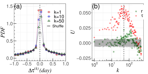
where when and otherwise it is zero. We exclude the zero increments from the calculation; the number of zero increments is indeed very small. is bounded between -1 (monotonically decreasing sequence) and 1 (monotonically increasing sequence). When is close to zero, the time series is symmetric (for example, the PDF is nearly symmetrical close to for but highly asymmetric for and in Figure 2(a)). For instance, if the asymmetry value of , the number of positive increments is twice the number of negative increments (i.e., =2). The positive (negative) increment of the interevent time represents the decreasing (increasing) earthquake rate. Similarly, we define the asymmetry of the interevent distance (in km) between the epicenters.
2.2 Generalized ETAS model
We also study the asymmetry of synthetic catalogs based on the ETAS model in comparison to the asymmetry observed in the time series of real records. We use the ETAS model as a null hypothesis , since it is the most widely used statistical model to simulate the spatiotemporal clustering of seismic events [Ogata (\APACyear1988), Ogata (\APACyear1998)]. The earthquake sequence in the ETAS is defined as a stochastic Hawkes (point) process. We use the Gutenberg–Richter law (where , truncated at ) to independently generate the magnitude of each earthquake (). For the ETAS model, the conditional intensity function (which is basically the rate of earthquakes) at time with the seismic history prior to is given by
| (2) |
where is the background rate to generate spontaneous earthquakes estimated from the real catalogs [Zhuang \BOthers. (\APACyear2010), Zhuang (\APACyear2012)]. The occurrence times of the past events are represented as , and their magnitudes are (). Future earthquakes can be triggered by each past earthquake according to the generalized triggering function which here includes two triggering processes [Zhang \BOthers. (\APACyear2021)], as
| (3) |
where is the total number of past events. The productivity of triggering earthquakes is controlled by the two productivity parameters and corresponding to the short-term () and long-term () triggering respectively, which satisfy . If the interevent number is smaller than the crossover number , the -th earthquake can be trigged by the -th historical earthquake with a higher rate according to the larger . The crossover number is equal to which is estimated from the memory measure of real earthquake catalog as reported by \citeAZhang2020. Also, we use the parameters in Eq. (3) estimated from real earthquake catalogs [Zhang \BOthers. (\APACyear2021)]. The generalized ETAS model reduces to the standard ETAS model if . We add only two parameters, and to the standard ETAS model and all other parameters remain the same. Note that when is different with , Eq. 3 is a discontinuous function. Yet, it is very hard to observe a systematical discontinuity in synthetic catalogs of the generalized ETAS model as well as real data, since the cascading triggering process of aftershocks can weaken the discontinuity [Zhang \BOthers. (\APACyear2021)].
2.3 Data
We analyze the Italian earthquake catalog between 1981 and 2017 [Gasperini \BOthers. (\APACyear2013)]. We also analyzed the Japan Unified High-Resolution Relocated Catalog for Earthquakes (JUICE) bewteen 2001 to 2012 [Yano \BOthers. (\APACyear2017)] and the Southern California catalog from 1981 to 2018 [Hauksson \BOthers. (\APACyear2012)]. The three catalogs are complete for magnitude threshold [Hauksson \BOthers. (\APACyear2012), Gasperini \BOthers. (\APACyear2013), Yano \BOthers. (\APACyear2017)] and this is also shown in Figure S1 where the distributions of the magnitudes () follow the Gutenberg-Richter law.
3 Results
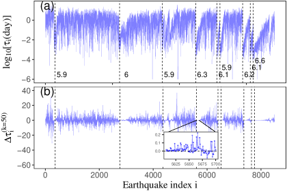
First, we obtain interevent times of the Italian earthquake catalog (using the threshold of magnitude ) and their increments for the lag index . The results are shown in Fig. 1. As can be seen, interevent times decrease abruptly and then increase gradually after the occurrence of a large earthquake (Fig 1(a)), consistent with the Omori law. The increments are very small immediately after large shocks even for , and most of them are positive (see inset figure) in Fig. 1(b). After sufficient time from a main shock, a crossover time, the rate of aftershocks decreases and the interevent increments become symmetric and switch between negative and positive values. Moreover, Fig. 1(b) shows that the interevent time increments for lag tend to be negative before the occurrence of large earthquakes. This observation can be explained as follows. The event time intervals before the main shock are relatively large in comparison to the event time intervals after the main shock, since the earthquake (aftershock) rate after the main shock is high. The difference between time interval for lag , , as approaching the main shock, involves the subtraction of a long-time interval before the main shock from a short time interval after the main shock, leading to negative . Thus, will be negative lags preceding the main shock.
Fig. 2(a) shows the Probability Density Function (PDF) of the interevent time increments for different . The PDFs are essentially asymmetric about when increases and the asymmetry is dominated by the points close to . To verify the significance of the asymmetry, we randomly shuffled the time series of interevent times and produced 100 shuffled sequences. This shuffling procedure destroys the (temporal) aftershock clustering such that the number of positive and negative increments should be similar. As a result, the number of small increments decreases and the number of large increments increases and the peak of the PDF (see gray shades in Fig. 2(a)) is much lower than the peak of the PDF of the original catalog. For a larger increment lag of , , the PDF becomes more asymmetric in comparison to PDF with and the PDF of the shuffled data [Fig.2(a)]. More positive increments are observed for the larger lag-index .
To quantify the level of the asymmetry, we calculate the measure as a function of lag-index using Eq. (1). Fig. 2(b) depicts, for the Italian catalog, the measure for the interevent times (red) as a function of the lag increment . The asymmetry measure, , increases with for below a crossover lag, , and decreases with above the crossover ; is maximal at the crossover until it is indistinguishable from the random process shown at high . As discussed above, we expect the presence of asymmetry in the interevent times following the Omori-law [Fig. 1 and Fig. 2(a)]. Yet, the non-monotonic behavior with maximal asymmetry at is not trivial which implies a transition between the effect of the Omori-law and a random process. We also calculated the asymmetry measure, , for interevent distances (green symbols in Fig. 2(b)) and observed similar behavior as for the interevent times, although much less pronounced. The results of shuffled, symmetric, time series (gray shaded area) are also included in Fig. 2(b) and indicate significant asymmetry for interevent times compared to this null hypothesis over a wide range of lags (). For interevent distances we observe weak asymmetry only around lag .
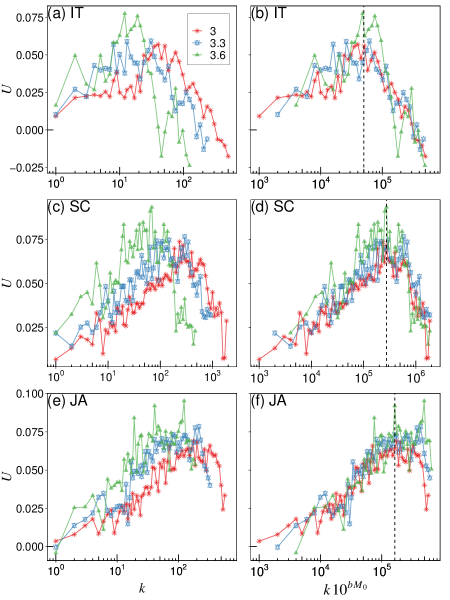
We also calculated the asymmetry measure, , for three magnitude thresholds and three places. Fig. 3(a), (c) and (e) show versus the index for the interevent times when using different magnitude thresholds , and for the catalogs of Italy (IT), Southern California (SC) and Japan (JA). The asymmetry measure, , exhibits similar increasing and decreasing trends for all three catalogs. The crossover lag, , (at which the asymmetry is maximal) is smaller for the larger magnitude threshold (see Fig. 3(a), (c) and (e)). According to the Gutenberg-Richter law, the number of earthquakes decreases exponentially with the increasing magnitude threshold. Thus, we rescale the lag with and the results are shown in Fig. 3(b), (d) and (f). The different asymmetry curves collapse into a single curve for which the crossover is ; this scaling approach is similar to the scaling procedure of interevent times discussed in previous studies [Bak \BOthers. (\APACyear2002), Corral (\APACyear2003), Saichev \BBA Sornette (\APACyear2006), Sornette \BOthers. (\APACyear2008)]. However, the crossovers are not the same for different places. For IT, the rescaled crossover lag is, and is smaller than the crossovers for JA () and SC (). The asymmetry curves also satisfy the scaling relation by rescaling the lag with the averaged time intervals as shown in Fig. S2. We thus obtain that the crossover times approximately correspond to 80, 280, and 50 days for IT, SC and JA respectively. We also consider and observed the asymmetry for different region sizes as shown in Fig. S3(a). A smaller region size shows a larger asymmetry since more events (aftershocks) are correlated within the area as proposed by \citeATouati2009. Moreover, the crossover can be scaled with respect to region size in Fig. S3(b). Figure S4 shows the weak asymmetry for the global earthquake catalog.
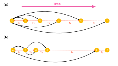
We now aim to explain the mechanism underlying the observed asymmetry measure. Considering a simple situation, for which aftershocks – are the first generation aftershocks triggered by a mainshock , as shown by the schematic drawing in Fig. 4(a). Due to the Omori law, the frequency of aftershocks decreases like ( is close to 1 and is the time since the mainshock) such that the interevent time after the mainshock follows . Thus, the interevent time statistically increases with time, resulting in a positive asymmetry with more positive increments in comparison to negative increments. However, the real situation is more complex as not only mainshocks can trigger aftershocks but aftershocks can also trigger other aftershocks. Moreover, spontaneous earthquakes (mainshocks) could be mixed with aftershocks due to the stacking involved (see the example in Fig. 4(b)). The indirect triggered events and the spontaneous events can decrease the interevent times as shown in Fig. 4(b) (, and are smaller than ). The above considerations implies that the events below the crossover lag are mainly triggered by a mainshock. Above the crossover (), the sequences for spontaneous and triggered events will overlap with high probabilities resulting in a fast decay of asymmetry.
The ETAS model is widely used to simulate and study the temporal clustering of seismic events [Ogata (\APACyear1988), Ogata (\APACyear1998)]. The rate function of the ETAS model consists of the spontaneous (background) rate and triggering rate of historical events (see Eq. (2)). The choice of parameters in the ETAS model is critical to reproduce the features of real earthquake sequences. The maximum likelihood estimation (MLE) procedure has been proposed [Zhuang \BOthers. (\APACyear2010)] to estimate the parameters. In a recent study [Zhang \BOthers. (\APACyear2021)] the conventional ETAS model has been found to be unable to reproduce important (long-term) memory characteristics observed in real catalogs. In the same study a generalized the ETAS model has been developed and found to be useful in reproducing the observe memory features that appear in the real catalogs (see Materials and Methods). Below we test the asymmetry of the generalized ETAS model for Italy with three choices of parameters: (I) such that the generalized model reduces to the standard ETAS model. The parameters are estimated using the MLE. This choice is termed “EM0”. (II) Since some studies have reported that the -value is underestimated by the MLE [Marzocchi \BBA Lombardi (\APACyear2009), Seif \BOthers. (\APACyear2017), Zhuang \BOthers. (\APACyear2019)], we consider a second choice of parameters termed “EM1”, which is the same as EM0 but with larger (and smaller to guarantee the similar branching ratio) (Eq. (3)). (III) The generalized ETAS model with developed recently [Zhang \BOthers. (\APACyear2021)]. This choice is termed “EM2”. The selected parameters of EM0, EM1 and EM2 for the Italian catalog are listed in Table 1. We generated 50 realizations of synthetic catalogs with magnitudes greater than or equal to magnitude 3, each covering 50000 days. The earthquake rates are 0.690.03, 0.730.1 and 0.710.06 events per day for EM0, EM1 and EM2 respectively. The rates of the models are similar and close to that of the real data.
| EM0 | 0.2 | 0.007 | 1.13 | 6.26 | 1.4 | 1.4 | – |
| EM1 | 0.2 | 0.007 | 1.13 | 2.91 | 2.0 | 2.0 | – |
| EM2 | 0.2 | 0.007 | 1.13 | 3.35 | 2.0 | 1.4 |
Next, we study the asymmetry for the three versions of the ETAS model introduced above. Figure 5(a) shows that the asymmetry of the interevent times in the standard ETAS, EM0, in marked contrast with real asymmetry, deceases with the lag index without a crossover for EM0 (green dots). Both, EM1 (red squares) and EM2 (green triangles) exhibit much better performance and their asymmetry curves are similar to the real catalog (dotted line). Due to the smaller in EM0 relative to EM1, the probability of aftershocks directly triggered by a large mainshock is too low to increase the asymmetry for EM0. Thus, the asymmetry deceases as the lag index increases at the beginning rather than after a certain lag. The asymmetry of EM0 demonstrates that the -value is indeed underestimated by MLE. Comparing between EM1 and EM2, the asymmetry of EM2 decays faster above the crossover, more similar to the decay of the real catalog, the dotted line (see Fig. 5(a)). Moreover, the crossover point is different for EM1 () and EM2 (). Thus, the crossover of EM2 is closer to the observed one (Fig. 5(a)). We thus conclude that the two-alpha () ETAS model exhibits the best performance in reproducing both the memory [Zhang \BOthers. (\APACyear2021)] and asymmetry in the current study than both versions of the standard ETAS model. The asymmetry of EM2 also satisfies the scaling relation for the magnitude threshold similar to the real one (see SI, Figure S5).
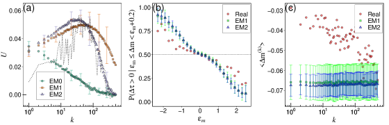
We further study the dependence of the interevent time increments on the magnitude increment , to understand in more details the role of Omori law on the asymmetry. For this purpose we calculated the conditional probability , where is the bin size of the magnitude increment. Figure 5(b) shows that this conditional probability decreases when the magnitude increment increases, for the real, EM1 and EM2 catalogs;. Moreover, the conditional probability is around 0.5 (corresponding to the asymmetry measure around zero) when is close to zero. Thus, the asymmetry measure close to zero could be due to the magnitude similarity for small lag-index , as the PDF interevent time increments is maximal close to zero (Fig 2(a)). Previous studies [Lippiello \BOthers. (\APACyear2008), Lippiello \BOthers. (\APACyear2012)] have found that the magnitude of consecutive events is more similar than would be expected from random sampling of the Gutenber-Richter distribution. It is apparent that EM1 and EM2 overestimate the conditional probability of the real data. Fig. 5(c) shows the average of the magnitude increment for days (to focus on aftershocks) as a function of the lag-index . The size of aftershock is usually smaller than the mainshock yielding the negative values in Figure 5(c). Yet, it is also clear that while the mean magnitude difference is almost constant with lag for EM1 and EM2, it decreases for the real catalog, from values closer to zero for small lag-index to values of EM1 and EM2 at large (Fig. 5(c)). These results indicate that the magnitude similarity reported by [Lippiello \BOthers. (\APACyear2008), Lippiello \BOthers. (\APACyear2012)] is absent in both models.
While the asymmetry of EM2 is similar to the asymmetry of the real catalog for , it is significantly higher for smaller (Fig. 5(a)). The Italian catalog we used has been reported to be complete above magnitude threshold 3.0. [Gasperini \BOthers. (\APACyear2013)]. However, due to the inefficiency of the seismic network and the overlapping of aftershock seismograms, an earthquake catalog could be incomplete, especially after mainshocks [Kagan (\APACyear2004), Hainzl (\APACyear2016), de Arcangelis \BOthers. (\APACyear2018)]. To investigate the effect of the incompleteness of the catalogs, we generate synthetic incomplete catalogs based on the studies of \citeAhelmstetter2006comparison,Seif2017,petrillo2021testing. The incomplete ETAS model is based on the conditional earthquake rate intensity function as [Petrillo \BBA Lippiello (\APACyear2021)],
| (4) |
where all past events with are considered. We define when , when , else. The magnitude threshold is calculated as [Kagan (\APACyear2004), Hainzl (\APACyear2016), de Arcangelis \BOthers. (\APACyear2018)],
| (5) |
where is the magnitude of past event , and is the time since the past event. The parameter is chosen following \citeApetrillo2021testing and \citeASeif2017,helmstetter2006comparison suggested the following parameter values and . We consider three different choices of the parameter , , , and to generate synthetic catalogs with different degree of incompleteness.
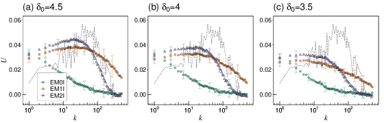
To generate the synthetic incomplete catalogs based on EM0, EM1 and EM2 (represented as EM0I, EM1I and EM2I respectively), we remove an aftershock from the synthetic complete catalogs with a probability given by [Petrillo \BBA Lippiello (\APACyear2021)]. To roughly preserve the total number of earthquakes to be the same as that of Figure 5(a), we increased slightly the parameter and left the other parameters unchanged. With this procedure, the level of incompleteness of each synthetic catalog was 5%, 10% and 20% for , , and respectively for EM1I and EM2I; the percentages indicate the relative number of events that has been removed from the complete catalog. It is apparent from our results (see Figure 6) that the asymmetry weakens as the degree of incompleteness is higher. Still, for both models, the asymmetry is overestimated for small lag index in comparison to the real catalog and weakens when the catalogs are more incomplete. Figure S6 shows similar results when using , , to control the degree of incompleteness. We also try to control the parameter to keep the same number of earthquakes for EM0I, EM1I and EM2I and the results are shown in Figure S7.
4 Conclusions
Here, we investigated the asymmetry behavior of interevent times (and distances) in earthquake catalogs. For real seismic catalogs, the asymmetry as a function of first increases up to a crossover lag and then decreases rapidly. The crossover lag changes with location and with the magnitude threshold, where the latter can be rescaled to unified value of . We suggest that the Omori law is associated with the increase of the asymmetry below the crossover and has a decreasing influence above this crossover. This is probably due to the overlapping of different triggered aftershocks and the spontaneous events that lead to a fast decay of asymmetry above the crossover. The de-clustering between spontaneous and triggered earthquake events is still an open important question [Zaliapin \BOthers. (\APACyear2008), Zaliapin \BBA Ben-Zion (\APACyear2013)]. The asymmetry results reported here and its associated crossover may help to resolve this question although this requires further investigation.
In the standard ETAS model whose parameters are estimated by MLE, the increase of asymmetry and the crossover cannot be reproduced. When the -value is increased, a large mainshock can trigger more aftershocks such that there exists an increasing trend and a crossover in the standard ETAS model. This demonstrates that the common -value is indeed underestimated by MLE. However, the crossover value of is larger and the asymmetry above the crossover is significantly higher and decays slower in the standard ETAS model with large than the real one. The generalized ETAS model with two -values () in short and long time scales exhibits similar asymmetry behavior as that of the real catalog for lags larger than the crossover lag . Yet, the asymmetry for small lag-index is overestimated by both models (one and two -value). We suggest that the short-term symmetrical behavior can be attributed to the magnitude similarity in real data which is missing in both models. The additional advantage of the generalized ETAS model is its ability to reproduce the observe memory in earthquake catalogs as reported in [Zhang \BOthers. (\APACyear2021)]. Thus, generally speaking, the asymmetry findings reported here may be used to improve earthquake forecasting models as the asymmetry measure can serve as an additional characteristic that a forecasting model should reproduce.
Acknowledgements.
We thank for the financial support by the EU H2020 project RISE, the Israel Science Foundation (Grants No. 189/19), DTRA ,the Pazy Foundation, the joint China-Israel Science Foundation (Grants No. 3132/19) and the BIU Center for Research in Applied Cryptography and Cyber Security. We thank the Israel ministry of energy. We downloaded the Southern California catalog from the SCEDC (https://scedc.caltech.edu/research-tools/alt-2011-dd-hauksson-yang-shearer.html) [Hauksson \BOthers. (\APACyear2012)] and the Japanese Catalog (JUICE) from ref [Yano \BOthers. (\APACyear2017)]. The Italian catalog is available on request from ref [Gasperini \BOthers. (\APACyear2013)] and the authors.References
- An (\APACyear2004) \APACinsertmetastarAn2004{APACrefauthors}An, S\BPBII. \APACrefYearMonthDay2004. \BBOQ\APACrefatitleInterdecadal changes in the El Nino-La Nina asymmetry Interdecadal changes in the El Nino-La Nina asymmetry.\BBCQ \APACjournalVolNumPagesGeophys. Res. Lett.31231–4. {APACrefDOI} 10.1029/2004GL021699 \PrintBackRefs\CurrentBib
- Ashkenazy \BOthers. (\APACyear2008) \APACinsertmetastarAshkenazy2008{APACrefauthors}Ashkenazy, Y., Feliks, Y., Gildor, H.\BCBL \BBA Tziperman, E. \APACrefYearMonthDay2008. \BBOQ\APACrefatitleAsymmetry of daily temperature records Asymmetry of daily temperature records.\BBCQ \APACjournalVolNumPagesJ. Atmos. Sci.65103327–3336. {APACrefDOI} 10.1175/2008JAS2662.1 \PrintBackRefs\CurrentBib
- Bak \BOthers. (\APACyear2002) \APACinsertmetastarBak2002{APACrefauthors}Bak, P., Christensen, K., Danon, L.\BCBL \BBA Scanlon, T. \APACrefYearMonthDay2002. \BBOQ\APACrefatitleUnified Scaling Law for Earthquakes Unified Scaling Law for Earthquakes.\BBCQ \APACjournalVolNumPagesPhys. Rev. Lett.8817178501. {APACrefDOI} 10.1103/PhysRevLett.88.178501 \PrintBackRefs\CurrentBib
- Corral (\APACyear2003) \APACinsertmetastarCorral2003{APACrefauthors}Corral, Á. \APACrefYearMonthDay2003. \BBOQ\APACrefatitleLocal distributions and rate fluctuations in a unified scaling law for earthquakes Local distributions and rate fluctuations in a unified scaling law for earthquakes.\BBCQ \APACjournalVolNumPagesPhys. Rev. E683035102. {APACrefDOI} 10.1103/PhysRevE.68.035102 \PrintBackRefs\CurrentBib
- Corral (\APACyear2004) \APACinsertmetastarCorral2003a{APACrefauthors}Corral, Á. \APACrefYearMonthDay2004. \BBOQ\APACrefatitleLong-Term Clustering, Scaling, and Universality in the Temporal Occurrence of Earthquakes Long-Term Clustering, Scaling, and Universality in the Temporal Occurrence of Earthquakes.\BBCQ \APACjournalVolNumPagesPhys. Rev. Lett.9210108501. {APACrefDOI} 10.1103/PhysRevLett.92.108501 \PrintBackRefs\CurrentBib
- Davidsen \BOthers. (\APACyear2007) \APACinsertmetastarDavidsen2007{APACrefauthors}Davidsen, J., Stanchits, S.\BCBL \BBA Dresen, G. \APACrefYearMonthDay2007. \BBOQ\APACrefatitleScaling and universality in rock fracture Scaling and universality in rock fracture.\BBCQ \APACjournalVolNumPagesPhys. Rev. Lett.9812125502. {APACrefDOI} 10.1103/PhysRevLett.98.125502 \PrintBackRefs\CurrentBib
- de Arcangelis \BOthers. (\APACyear2016) \APACinsertmetastarDeArcangelis2016{APACrefauthors}de Arcangelis, L., Godano, C., Grasso, J\BPBIR.\BCBL \BBA Lippiello, E. \APACrefYearMonthDay2016. \BBOQ\APACrefatitleStatistical physics approach to earthquake occurrence and forecasting Statistical physics approach to earthquake occurrence and forecasting.\BBCQ \APACjournalVolNumPagesPhys. Rep.6281–91. {APACrefDOI} 10.1016/j.physrep.2016.03.002 \PrintBackRefs\CurrentBib
- de Arcangelis \BOthers. (\APACyear2018) \APACinsertmetastarDeArcangelis2018{APACrefauthors}de Arcangelis, L., Godano, C.\BCBL \BBA Lippiello, E. \APACrefYearMonthDay2018. \BBOQ\APACrefatitleThe Overlap of Aftershock Coda Waves and Short-Term Postseismic Forecasting The Overlap of Aftershock Coda Waves and Short-Term Postseismic Forecasting.\BBCQ \APACjournalVolNumPagesJ. Geophys. Res. Solid Earth12375661–5674. {APACrefDOI} 10.1029/2018JB015518 \PrintBackRefs\CurrentBib
- Fan \BOthers. (\APACyear2019) \APACinsertmetastarFan2018b{APACrefauthors}Fan, J., Zhou, D., Shekhtman, L\BPBIM., Shapira, A., Hofstetter, R., Marzocchi, W.\BDBLHavlin, S. \APACrefYearMonthDay2019. \BBOQ\APACrefatitlePossible origin of memory in earthquakes: Real catalogs and an epidemic-type aftershock sequence model Possible origin of memory in earthquakes: Real catalogs and an epidemic-type aftershock sequence model.\BBCQ \APACjournalVolNumPagesPhys. Rev. E994042210. {APACrefDOI} 10.1103/PhysRevE.99.042210 \PrintBackRefs\CurrentBib
- Gasperini \BOthers. (\APACyear2013) \APACinsertmetastarGasperini2013{APACrefauthors}Gasperini, P., Lolli, B.\BCBL \BBA Vannucci, G. \APACrefYearMonthDay2013. \BBOQ\APACrefatitleEmpirical calibration of local magnitude data sets versus moment magnitude in Italy Empirical calibration of local magnitude data sets versus moment magnitude in Italy.\BBCQ \APACjournalVolNumPagesBull. Seismol. Soc. Am.10342227–2246. {APACrefDOI} 10.1785/0120120356 \PrintBackRefs\CurrentBib
- Gutenberg \BBA Richter (\APACyear1944) \APACinsertmetastarGutenberg1944a{APACrefauthors}Gutenberg, B.\BCBT \BBA Richter, C\BPBIF. \APACrefYearMonthDay1944. \BBOQ\APACrefatitleFrequency of Earthquakes in California Frequency of Earthquakes in California.\BBCQ \APACjournalVolNumPagesBull. Seismol. Soc. Am.344185–188. {APACrefDOI} 10.1038/156371a0 \PrintBackRefs\CurrentBib
- Hainzl (\APACyear2016) \APACinsertmetastarHainzl2016{APACrefauthors}Hainzl, S. \APACrefYearMonthDay2016. \BBOQ\APACrefatitleRate‐Dependent Incompleteness of Earthquake Catalogs Rate‐Dependent Incompleteness of Earthquake Catalogs.\BBCQ \APACjournalVolNumPagesSeismol. Res. Lett.872A337–344. {APACrefDOI} 10.1785/0220150211 \PrintBackRefs\CurrentBib
- Hauksson \BOthers. (\APACyear2012) \APACinsertmetastarHauksson2012{APACrefauthors}Hauksson, E., Yang, W.\BCBL \BBA Shearer, P\BPBIM. \APACrefYearMonthDay2012. \BBOQ\APACrefatitleWaveform Relocated Earthquake Catalog for Southern California (1981 to June 2011) Waveform Relocated Earthquake Catalog for Southern California (1981 to June 2011).\BBCQ \APACjournalVolNumPagesBull. Seismol. Soc. Am.10252239–2244. {APACrefDOI} 10.1785/0120120010 \PrintBackRefs\CurrentBib
- Helmstetter \BOthers. (\APACyear2006) \APACinsertmetastarhelmstetter2006comparison{APACrefauthors}Helmstetter, A., Kagan, Y\BPBIY.\BCBL \BBA Jackson, D\BPBID. \APACrefYearMonthDay2006. \BBOQ\APACrefatitleComparison of short-term and time-independent earthquake forecast models for southern California Comparison of short-term and time-independent earthquake forecast models for southern california.\BBCQ \APACjournalVolNumPagesBull. Seismol. Soc. Am.96190–106. \PrintBackRefs\CurrentBib
- Hoyt \BBA Schatten (\APACyear1998) \APACinsertmetastarhoyt1998group{APACrefauthors}Hoyt, D\BPBIV.\BCBT \BBA Schatten, K\BPBIH. \APACrefYearMonthDay1998. \BBOQ\APACrefatitleGroup sunspot numbers: A new solar activity reconstruction Group sunspot numbers: A new solar activity reconstruction.\BBCQ \APACjournalVolNumPagesSol. Phys1791189–219. \PrintBackRefs\CurrentBib
- Huc \BBA Main (\APACyear2003) \APACinsertmetastarHuc2003{APACrefauthors}Huc, M.\BCBT \BBA Main, I\BPBIG. \APACrefYearMonthDay2003. \BBOQ\APACrefatitleAnomalous stress diffusion in earthquake triggering: Correlation length, time dependence, and directionality Anomalous stress diffusion in earthquake triggering: Correlation length, time dependence, and directionality.\BBCQ \APACjournalVolNumPagesJ. Geophys. Res. Solid Earth108B7. {APACrefDOI} 10.1029/2001jb001645 \PrintBackRefs\CurrentBib
- Hutchinson \BOthers. (\APACyear2013) \APACinsertmetastarHutchinson2013{APACrefauthors}Hutchinson, D\BPBIK., England, M\BPBIH., Santoso, A.\BCBL \BBA Hogg, A\BPBIM\BPBIC. \APACrefYearMonthDay2013. \BBOQ\APACrefatitleInterhemispheric asymmetry in transient global warming: The role of Drake Passage Interhemispheric asymmetry in transient global warming: The role of Drake Passage.\BBCQ \APACjournalVolNumPagesGeophys. Res. Lett.4081587–1593. {APACrefDOI} 10.1002/grl.50341 \PrintBackRefs\CurrentBib
- Ide (\APACyear2013) \APACinsertmetastarIde2013{APACrefauthors}Ide, S. \APACrefYearMonthDay2013. \BBOQ\APACrefatitleThe proportionality between relative plate velocity and seismicity in subduction zones The proportionality between relative plate velocity and seismicity in subduction zones.\BBCQ \APACjournalVolNumPagesNat. Geosci.69780–784. {APACrefDOI} 10.1038/ngeo1901 \PrintBackRefs\CurrentBib
- Jordan \BOthers. (\APACyear2011) \APACinsertmetastarjordan2011operational{APACrefauthors}Jordan, T\BPBIH., Chen, Y\BHBIT., Gasparini, P., Madariaga, R., Main, I., Marzocchi, W.\BDBLZschau, J. \APACrefYearMonthDay2011. \BBOQ\APACrefatitleOperational earthquake forecasting. State of knowledge and guidelines for utilization Operational earthquake forecasting. state of knowledge and guidelines for utilization.\BBCQ \APACjournalVolNumPagesAnn. Geophys.544361–391. \PrintBackRefs\CurrentBib
- Kagan (\APACyear2004) \APACinsertmetastarKagan2004{APACrefauthors}Kagan, Y\BPBIY. \APACrefYearMonthDay2004. \BBOQ\APACrefatitleShort-term properties of earthquake catalogs and models of earthquake source Short-term properties of earthquake catalogs and models of earthquake source.\BBCQ \APACjournalVolNumPagesBull. Seismol. Soc. Am.9441207–1228. {APACrefDOI} 10.1785/012003098 \PrintBackRefs\CurrentBib
- King (\APACyear1996) \APACinsertmetastarKing1996{APACrefauthors}King, T. \APACrefYearMonthDay1996. \BBOQ\APACrefatitleQuantifying nonlinearity and geometry in time series of climate Quantifying nonlinearity and geometry in time series of climate.\BBCQ \APACjournalVolNumPagesQuat. Sci. Rev.154247–266. {APACrefDOI} 10.1016/0277-3791(95)00060-7 \PrintBackRefs\CurrentBib
- Lennartz \BOthers. (\APACyear2008) \APACinsertmetastarLennartz2008{APACrefauthors}Lennartz, S., Livina, V\BPBIN., Bunde, A.\BCBL \BBA Havlin, S. \APACrefYearMonthDay2008. \BBOQ\APACrefatitleLong-term memory in earthquakes and the distribution of interoccurrence times Long-term memory in earthquakes and the distribution of interoccurrence times.\BBCQ \APACjournalVolNumPagesEPL8163–7. {APACrefDOI} 10.1209/0295-5075/81/69001 \PrintBackRefs\CurrentBib
- Lippiello \BOthers. (\APACyear2008) \APACinsertmetastarLippiello2008{APACrefauthors}Lippiello, E., De Arcangelis, L.\BCBL \BBA Godano, C. \APACrefYearMonthDay2008. \BBOQ\APACrefatitleInfluence of time and space correlations on earthquake magnitude Influence of time and space correlations on earthquake magnitude.\BBCQ \APACjournalVolNumPagesPhys. Rev. Lett.10031–4. {APACrefDOI} 10.1103/PhysRevLett.100.038501 \PrintBackRefs\CurrentBib
- Lippiello \BOthers. (\APACyear2009) \APACinsertmetastarLippiello2009a{APACrefauthors}Lippiello, E., De Arcangelis, L.\BCBL \BBA Godano, C. \APACrefYearMonthDay2009. \BBOQ\APACrefatitleRole of static stress diffusion in the spatiotemporal organization of aftershocks Role of static stress diffusion in the spatiotemporal organization of aftershocks.\BBCQ \APACjournalVolNumPagesPhys. Rev. Lett.1033. {APACrefDOI} 10.1103/PhysRevLett.103.038501 \PrintBackRefs\CurrentBib
- Lippiello \BOthers. (\APACyear2012) \APACinsertmetastarLippiello2012{APACrefauthors}Lippiello, E., Godano, C.\BCBL \BBA De Arcangelis, L. \APACrefYearMonthDay2012. \BBOQ\APACrefatitleThe earthquake magnitude is influenced by previous seismicity The earthquake magnitude is influenced by previous seismicity.\BBCQ \APACjournalVolNumPagesGeophys. Res. Lett.395. {APACrefDOI} 10.1029/2012GL051083 \PrintBackRefs\CurrentBib
- Livina \BOthers. (\APACyear2003) \APACinsertmetastarLivina2003a{APACrefauthors}Livina, V\BPBIN., Ashkenazy, Y., Braun, P., Monetti, R., Bunde, A.\BCBL \BBA Havlin, S. \APACrefYearMonthDay2003. \BBOQ\APACrefatitleNonlinear volatility of river flux fluctuations Nonlinear volatility of river flux fluctuations.\BBCQ \APACjournalVolNumPagesPhys. Rev. E6744. {APACrefDOI} 10.1103/PhysRevE.67.042101 \PrintBackRefs\CurrentBib
- Livina \BOthers. (\APACyear2005) \APACinsertmetastarLivina2005{APACrefauthors}Livina, V\BPBIN., Havlin, S.\BCBL \BBA Bunde, A. \APACrefYearMonthDay2005. \BBOQ\APACrefatitleMemory in the Occurrence of Earthquakes Memory in the Occurrence of Earthquakes.\BBCQ \APACjournalVolNumPagesPhys. Rev. Lett.9520208501. {APACrefDOI} 10.1103/PhysRevLett.95.208501 \PrintBackRefs\CurrentBib
- Lombardi (\APACyear2015) \APACinsertmetastarLombardi2015{APACrefauthors}Lombardi, A\BPBIM. \APACrefYearMonthDay2015. \BBOQ\APACrefatitleEstimation of the parameters of ETAS models by Simulated Annealing Estimation of the parameters of ETAS models by Simulated Annealing.\BBCQ \APACjournalVolNumPagesSci. Rep.518417. {APACrefDOI} 10.1038/srep08417 \PrintBackRefs\CurrentBib
- Marsan \BBA Lengliné (\APACyear2008) \APACinsertmetastarMarsan2008{APACrefauthors}Marsan, D.\BCBT \BBA Lengliné, O. \APACrefYearMonthDay2008. \BBOQ\APACrefatitleExtending earthquakes’ reach through cascading Extending earthquakes’ reach through cascading.\BBCQ \APACjournalVolNumPagesScience31958661076–1079. {APACrefDOI} 10.1126/science.1148783 \PrintBackRefs\CurrentBib
- Marzocchi \BBA Lombardi (\APACyear2009) \APACinsertmetastarMarzocchi2009{APACrefauthors}Marzocchi, W.\BCBT \BBA Lombardi, A\BPBIM. \APACrefYearMonthDay2009. \BBOQ\APACrefatitleReal-time forecasting following a damaging earthquake Real-time forecasting following a damaging earthquake.\BBCQ \APACjournalVolNumPagesGeophys. Res. Lett.3621. {APACrefDOI} 10.1029/2009GL040233 \PrintBackRefs\CurrentBib
- Ogata (\APACyear1988) \APACinsertmetastarOgata1988{APACrefauthors}Ogata, Y. \APACrefYearMonthDay1988. \BBOQ\APACrefatitleStatistical Models for Earthquake Occurrences and Residual Analysis for Point Processes Statistical Models for Earthquake Occurrences and Residual Analysis for Point Processes.\BBCQ \APACjournalVolNumPagesJ. Am. Stat. Assoc.834019–27. {APACrefDOI} 10.1080/01621459.1988.10478560 \PrintBackRefs\CurrentBib
- Ogata (\APACyear1998) \APACinsertmetastarOgata1998{APACrefauthors}Ogata, Y. \APACrefYearMonthDay1998. \BBOQ\APACrefatitleSpace-Time Point-Process Models for Earthquake Occurrences Space-Time Point-Process Models for Earthquake Occurrences.\BBCQ \APACjournalVolNumPagesAnn. Inst. Stat. Math.502379–402. {APACrefDOI} 10.1023/A:1003403601725 \PrintBackRefs\CurrentBib
- Petrillo \BBA Lippiello (\APACyear2021) \APACinsertmetastarpetrillo2021testing{APACrefauthors}Petrillo, G.\BCBT \BBA Lippiello, E. \APACrefYearMonthDay2021. \BBOQ\APACrefatitleTesting of the foreshock hypothesis within an epidemic like description of seismicity Testing of the foreshock hypothesis within an epidemic like description of seismicity.\BBCQ \APACjournalVolNumPagesGeophys. J. Int.22521236–1257. \PrintBackRefs\CurrentBib
- Richards-Dinger \BOthers. (\APACyear2010) \APACinsertmetastarFelzer{APACrefauthors}Richards-Dinger, K., Stein, R\BPBIS.\BCBL \BBA Toda, S. \APACrefYearMonthDay2010. \BBOQ\APACrefatitleDecay of aftershock density with distance does not indicate triggering by dynamic stress Decay of aftershock density with distance does not indicate triggering by dynamic stress.\BBCQ \APACjournalVolNumPagesNature4677315583–586. {APACrefDOI} 10.1038/nature09402 \PrintBackRefs\CurrentBib
- Saichev \BBA Sornette (\APACyear2006) \APACinsertmetastarSaichev2006{APACrefauthors}Saichev, A.\BCBT \BBA Sornette, D. \APACrefYearMonthDay2006. \BBOQ\APACrefatitle“Universal” Distribution of Interearthquake Times Explained “Universal” Distribution of Interearthquake Times Explained.\BBCQ \APACjournalVolNumPagesPhys. Rev. Lett.977078501. {APACrefDOI} 10.1103/PhysRevLett.97.078501 \PrintBackRefs\CurrentBib
- Schreiber \BBA Schmitz (\APACyear1996) \APACinsertmetastarSchreiber1996{APACrefauthors}Schreiber, T.\BCBT \BBA Schmitz, A. \APACrefYearMonthDay1996. \BBOQ\APACrefatitleImproved surrogate data for nonlinearity tests Improved surrogate data for nonlinearity tests.\BBCQ \APACjournalVolNumPagesPhys. Rev. Lett.774635–638. {APACrefDOI} 10.1103/PhysRevLett.77.635 \PrintBackRefs\CurrentBib
- Seif \BOthers. (\APACyear2017) \APACinsertmetastarSeif2017{APACrefauthors}Seif, S., Mignan, A., Zechar, J\BPBID., Werner, M\BPBIJ.\BCBL \BBA Wiemer, S. \APACrefYearMonthDay2017. \BBOQ\APACrefatitleEstimating ETAS: The effects of truncation, missing data, and model assumptions Estimating ETAS: The effects of truncation, missing data, and model assumptions.\BBCQ \APACjournalVolNumPagesJ. Geophys. Res. Solid Earth1221449–469. {APACrefDOI} 10.1002/2016JB012809 \PrintBackRefs\CurrentBib
- Sornette \BOthers. (\APACyear2008) \APACinsertmetastarSornette2008{APACrefauthors}Sornette, D., Utkin, S.\BCBL \BBA Saichev, A. \APACrefYearMonthDay2008. \BBOQ\APACrefatitleSolution of the nonlinear theory and tests of earthquake recurrence times Solution of the nonlinear theory and tests of earthquake recurrence times.\BBCQ \APACjournalVolNumPagesPhys. Rev. E7761–10. {APACrefDOI} 10.1103/PhysRevE.77.066109 \PrintBackRefs\CurrentBib
- Touati \BOthers. (\APACyear2009) \APACinsertmetastarTouati2009{APACrefauthors}Touati, S., Naylor, M.\BCBL \BBA Main, I\BPBIG. \APACrefYearMonthDay2009. \BBOQ\APACrefatitleOrigin and Nonuniversality of the Earthquake Interevent Time Distribution Origin and Nonuniversality of the Earthquake Interevent Time Distribution.\BBCQ \APACjournalVolNumPagesPhys. Rev. Lett.10216168501. {APACrefDOI} 10.1103/PhysRevLett.102.168501 \PrintBackRefs\CurrentBib
- Utsu (\APACyear1961) \APACinsertmetastarUtsu1961{APACrefauthors}Utsu, T. \APACrefYearMonthDay1961. \BBOQ\APACrefatitleA statistical study on the occurrence of af- tershocks A statistical study on the occurrence of af- tershocks.\BBCQ \APACjournalVolNumPagesGeophys. Mag.30521–605. \PrintBackRefs\CurrentBib
- Utsu (\APACyear1972) \APACinsertmetastarUTSU1972{APACrefauthors}Utsu, T. \APACrefYearMonthDay1972. \BBOQ\APACrefatitleAftershocks and Earthquake Statistics (3) : Analyses of the Distribution of Earthquakes in Magnitude, Time and Space with Special Consideration to Clustering Characteristics of Earthquake Occurrence(1) Aftershocks and Earthquake Statistics (3) : Analyses of the Distribution of Earthquakes in Magnitude, Time and Space with Special Consideration to Clustering Characteristics of Earthquake Occurrence(1).\BBCQ \APACjournalVolNumPagesJ. Fac. Sci. Hokkaido Univ. Ser. 7, Geophys.411–42. \PrintBackRefs\CurrentBib
- Woessner \BOthers. (\APACyear2010) \APACinsertmetastarWoessner2010{APACrefauthors}Woessner, J., Christophersen, A., Douglas Zechar, J.\BCBL \BBA Monelli, D. \APACrefYearMonthDay2010. \BBOQ\APACrefatitleBuilding self-consistent, short-term earthquake probability (STEP) models: Improved strategies and calibration procedures Building self-consistent, short-term earthquake probability (STEP) models: Improved strategies and calibration procedures.\BBCQ \APACjournalVolNumPagesAnn. Geophys.533141–154. {APACrefDOI} 10.4401/ag-4812 \PrintBackRefs\CurrentBib
- Yano \BOthers. (\APACyear2017) \APACinsertmetastarYano2017{APACrefauthors}Yano, T\BPBIE., Takeda, T., Matsubara, M.\BCBL \BBA Shiomi, K. \APACrefYearMonthDay2017. \BBOQ\APACrefatitleJapan unified hIgh-resolution relocated catalog for earthquakes (JUICE): Crustal seismicity beneath the Japanese Islands Japan unified hIgh-resolution relocated catalog for earthquakes (JUICE): Crustal seismicity beneath the Japanese Islands.\BBCQ \APACjournalVolNumPagesTectonophysics70219–28. {APACrefDOI} 10.1016/j.tecto.2017.02.017 \PrintBackRefs\CurrentBib
- Zaliapin \BBA Ben-Zion (\APACyear2013) \APACinsertmetastarYehuda2013{APACrefauthors}Zaliapin, I.\BCBT \BBA Ben-Zion, Y. \APACrefYearMonthDay2013. \BBOQ\APACrefatitleEarthquake clusters in southern California I: Identification and stability Earthquake clusters in southern California I: Identification and stability.\BBCQ \APACjournalVolNumPagesJ. Geophys. Res. Solid Earth11862847–2864. {APACrefDOI} 10.1002/jgrb.50179 \PrintBackRefs\CurrentBib
- Zaliapin \BOthers. (\APACyear2008) \APACinsertmetastarZaliapin2008{APACrefauthors}Zaliapin, I., Gabrielov, A., Keilis-Borok, V.\BCBL \BBA Wong, H. \APACrefYearMonthDay2008. \BBOQ\APACrefatitleClustering analysis of seismicity and aftershock identification Clustering analysis of seismicity and aftershock identification.\BBCQ \APACjournalVolNumPagesPhys. Rev. Lett.10114–7. {APACrefDOI} 10.1103/PhysRevLett.101.018501 \PrintBackRefs\CurrentBib
- Zhang \BOthers. (\APACyear2020) \APACinsertmetastarZhang2019{APACrefauthors}Zhang, Y., Fan, J., Marzocchi, W., Shapira, A., Hofstetter, R., Havlin, S.\BCBL \BBA Ashkenazy, Y. \APACrefYearMonthDay2020. \BBOQ\APACrefatitleScaling laws in earthquake memory for interevent times and distances Scaling laws in earthquake memory for interevent times and distances.\BBCQ \APACjournalVolNumPagesPhys. Rev. Res.21013264. {APACrefDOI} 10.1103/PhysRevResearch.2.013264 \PrintBackRefs\CurrentBib
- Zhang \BOthers. (\APACyear2021) \APACinsertmetastarZhang2020{APACrefauthors}Zhang, Y., Zhou, D., Fan, J., Marzocchi, W., Ashkenazy, Y.\BCBL \BBA Havlin, S. \APACrefYearMonthDay2021. \BBOQ\APACrefatitleImproved earthquake aftershocks forecasting model based on long-term memory Improved earthquake aftershocks forecasting model based on long-term memory.\BBCQ \APACjournalVolNumPagesNew J. Phys23042001. {APACrefDOI} 10.1088/1367-2630/abeb46 \PrintBackRefs\CurrentBib
- Zhuang (\APACyear2012) \APACinsertmetastarZhuang2012{APACrefauthors}Zhuang, J. \APACrefYearMonthDay2012. \BBOQ\APACrefatitleLong-term earthquake forecasts based on the epidemic-type aftershock sequence (ETAS) model for short-term clustering Long-term earthquake forecasts based on the epidemic-type aftershock sequence (ETAS) model for short-term clustering.\BBCQ \APACjournalVolNumPagesRes. Geophys.218. {APACrefDOI} 10.4081/rg.2012.e8 \PrintBackRefs\CurrentBib
- Zhuang \BOthers. (\APACyear2019) \APACinsertmetastarZhuang2019{APACrefauthors}Zhuang, J., Murru, M., Falcone, G.\BCBL \BBA Guo, Y. \APACrefYearMonthDay2019. \BBOQ\APACrefatitleAn extensive study of clustering features of seismicity in Italy from 2005 to 2016 An extensive study of clustering features of seismicity in Italy from 2005 to 2016.\BBCQ \APACjournalVolNumPagesGeophys. J. Int.2161302–318. {APACrefDOI} 10.1093/gji/ggy428 \PrintBackRefs\CurrentBib
- Zhuang \BOthers. (\APACyear2010) \APACinsertmetastarZhuang2010{APACrefauthors}Zhuang, J., Werner, M\BPBIJ., Harte, D., Hainzl, S.\BCBL \BBA Zhou, S. \APACrefYearMonthDay2010. \BBOQ\APACrefatitleBasic models of seismicity Basic models of seismicity.\BBCQ \APACjournalVolNumPagesCommunity Online Resour. Stat. Seism. Anal.2–41. {APACrefDOI} 10.5078/corssa-47845067. \PrintBackRefs\CurrentBib