Piecewise Linear De-skewing for LiDAR Inertial Odometry

Abstract

Light detection and ranging (LiDAR) on a moving agent could suffer from motion distortion due to simultaneous rotation of the LiDAR and fast movement of the agent. An accurate piecewise linear de-skewing algorithm is proposed to correct the motion distortions for LiDAR inertial odometry (LIO) using high frequency motion information provided by an Inertial Measurement Unit (IMU). Experimental results show that the proposed algorithm can be adopted to improve the performance of existing LIO algorithms especially in cases of fast movement.

I Introduction

On-line localization of mobile agents plays an important role in autonomous navigation and it has been intensively studied for many years [1, 2, 3, 4, 5]. Since a light detection and ranging (LiDAR) rangefinder can provide highly reliable and precise distance measurements for surrounding environments and it is insensitive to ambient lighting and optical texture in a scene, the LiDAR rangefinder is one of the most widely adopted sensors for the indoor navigation among all available sensors [6, 7, 8]. Pose of a rangefinder can be estimated by matching two different scans [9]. Iterative Closest Point (ICP) algorithm is one of the dominant solutions for the scan matching problem [10, 11]. In existing ICP algorithms [10, 11, 12, 13, 14], the rotation of a laser beam is assumed to be the only motion of a scanning device. However, the rangefinder mounted on an autonomous vehicle or an unmanned aerial vehicle (UAV) usually moves during scanning a sweep due to movement of the agent. This introduces motion distortions among all points in the sweep, especially when the agent is moving fast.

Distortion caused by the movement of the agent affects accuracy of LiDAR odometry (LO). This problem was addressed by Bezet and Cherfaoui [15] in terms of time error correction. It is assumed that the sensor measures the distance to the same object between two frame at a same angle. The algorithm in [15] is not applicable if the agent rotates and moves fast. Zhang et al. [16] proposed an interesting LO algorithm by computing the transformation matrix from the first point to the last point of a sweep and linearly interpolating a transformation matrix to correct motion distortion for each point in the sweep. Accurate LO requires knowledge of the LiDAR pose during continuous laser ranging to correct the motion distortion. Fortunately, the knowledge can be provided by an IMU. The linear acceleration from IMU was also utilized in [16] to address the nonlinear motion of the agent. Experimental results indicate that the performance of the ICP can indeed be improved using the IMU measurements. Ye et al. [17] proposed an interesting de-skewing algorithm by using the IMU measurements. The transformation matrix from the first point to the last point of a sweep was first computed by using all the IMU measurements during the sweep. A transformation matrix is then linearly interpolated to correct the motion distortion for each point in the sweep. Same as [16], the movement of the agent was assumed to be linear during the sweep. The linear assumption is not true if the motion of the agent is complicated. For example, a sweep can be scanned when the agent goes straight and followed by a turn. It is desired to develop a new de-skewing algorithm without the linear assumption required by [16, 17]. Moreover, high accuracy preintegrated IMU models were proposed recently [1, 18, 19, 20]. All these models are derived for the moving agents where IMU pre-integration is considered in the world reference frame. On the other hand, the skewing distortion of 3D points occurs on the body frame. Therefore, the IMU pre-integration of 3D points in the body frame is worthy of being studied when the de-skewing of LiDAR scans is studied.

In this paper, an accurate piecewise linear de-skewing algorithm is proposed to correct motion distortions caused by the movement of the agent. The proposed algorithm is based on an observation that the IMU has a potential to provide the knowledge of the LiDAR pose during continuous laser ranging due to its high sampling rate. An elegant discrete model is first derived for a static 3D point of the environment in the body frame under the same assumption in [1, 18, 19], i.e., the linear acceleration and the angular velocity in the IMU frame are constant between two successive IMU measurements. The derivations in the body frame are much simpler than those in the world reference frame [1, 18, 19]. The new model is applied to derive a closed form IMU integration model for the static 3D point in the body frame. The proposed IMU motion integration model is different from the models in [1, 18, 19] in the sense that only the proposed model is on the static 3D point. Finally the proposed IMU integration model is adopted to correct the motion distortions caused by the movement of the agent. One point in a sweep is selected as the referencing point and each point in the sweep is corrected by using a transformation matrix which is computed by using all the IMU measurements between the referencing point and the point. Clearly, the proposed algorithm does not assume the motion of the agent to be linear during the sweep as required by [16, 17]. The corrected scans serve as the inputs of an existing LIO such as [17]. The proposed motion integration model is integrated with the LiDAR factor via a joint optimization with the mean measurement, the covariance matrix and the Jacobian matrix of the proposed model in [18]. As such, the proposed piecewise linear de-skewing algorithm and the LIO are seamlessly integrated together to reduce the motion distortion caused by the movement of the agent. The proposed de-skewing algorithm is complimentary to the existing LIO algorithms such as [17] and it can be used to improved the robustness of the existing LIO algorithms. Overall, two major contributions of this paper are: 1) an elegant closed form IMU integration model in the body frame for the static 3D point by using the IMU measurements, and 2) a piecewise linear de-skewing algorithm for correcting the motion distortion of the LiDAR which can be adopted by any existing LIO algorithm.

The rest of the paper is organized as follows. A literature review of related works is provided in Section II. Section III includes an IMU integration model for the 3D point, and section IV introduces the proposed de-skewing algorithm. Extensive results are given in Section V to verify the proposed algorithm. Finally, some conclusion remarks are provided in Section VI.

II Related Works

The existing ICP algorithms [10, 11, 12, 13, 14, 21] assume the rotation of a laser beam to be the only motion of a scanning device. Unfortunately, this is not always true [22]. An example is illustrated in Figure 1. The black line in Figure 1 represents an environment and the movement of the rangefinder is indicated by the green arrow while the red points are the raw scan data. Obviously, the set of the points is distorted due to the movement of the agent.

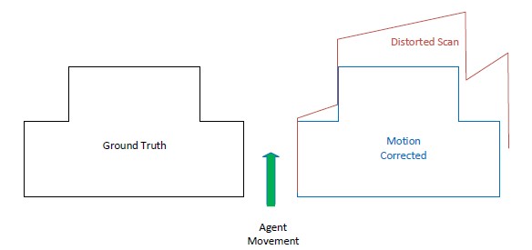
Figure 1: Motion distortions in a sweep of LiDAR. Black points is a given an environment, red points stand for a distorted scan, and blue points are a motion corrected scan.

Accurate LO requires knowledge of the LiDAR pose during continuous laser ranging to correct the motion distortion, and the knowledge can be provided by an IMU. The LiDAR and IMU measurements could be loosely coupled. Zhang et al. [16, 23] calculated the orientation of the robot pose by IMU measurements in LiDAR odometry and mapping (LOAM) algorithm. The LOAM considers the IMU measurements as a prior factor only for the algorithm. As a result, the IMU measurements were not used in the optimization process. Tang et al. [24] proposed to fuse the LiDAR and IMU measurements using an Extended Kalman filter (EKF). However, this algorithm was proposed for 2D scenarios and it is not applicable for a 3D environment. Lynen et al. [25] proposed a robust multi-sensors fusion approach which is applicable to the 3D environment. The LiDAR and IMU measurements were also fused using the EKF. Generally, the loosely coupled paradigms are simpler but less accurate.

The LiDAR and IMU measurements can also be tightly coupled. Soloviev et al. [26] proposed an algorithm for 2D LiDAR scanning and matching. IMU orientation measurements were used to compensate the tilted LiDAR. Moreover, the drift in IMU measurements was corrected and updated using the Kalman filter (KF). One more tightly coupled algorithm was proposed by Hemann et al. [27]. The algorithm can be applied to achieve good and robust results over long travelling period. However, it could fail without prior information about the environment. Inspired by the work in [28], Ye et al. [17] proposed a 3D tightly coupled fusion algorithm between the LiDAR and IMU measurements. One common way to address the motion distortion is the continuous-time representation such as the work in [29, 30]. Another technique is the linear interpolation approach [16]. The movement of the agent was assumed to be linear during the sweep. Its accuracy could be hindered by the linear motion assumption. It is thus desired to design a new de-skewing algorithm in order to compensate the motion distortion by using the high frequency IMU measurements.

III IMU Pre-integration of 3D Points

In this section, a new discrete motion pre-integration model is introduced for static 3D points of the environment in the LiDAR frame. Same as [1, 18], the proposed model assumes that both the linear acceleration and the angular velocity in the IMU frame are constant between two successive IMU measurements. It is worth noting that $a_{b}$ and $\omega_{b}$ can be derived by multiplying the readouts of the IMU by the fixed rotational matrix between the IMU and LiDAR. All notations of the proposed model are included in Table I.

TABLE I: Notations used in the proposed motion pre-integration model

$V_{b}=\left[\begin{array}[]{lll}V_{x}&V_{y}&V_{z}\end{array}\right]^{T}$	linear velocity of the
	agent in the LIDAR frame
$R_{bw}=\left[\begin{array}[]{lll}R_{1}&R_{2}&R_{3}\end{array}\right]$	rotation matrix from the world
	frame to the LIDAR frame
$a_{b}$	linear acceleration of the agent
	in the LIDAR frame
$g$	gravitational acceleration
$\omega_{b}=\left[\begin{array}[]{lll}\omega_{x}&\omega_{y}&\omega_{z}\end{array}\right]^{T}$	angular velocity of the agent
	in the LIDAR frame
$P_{b,l}=\left[\begin{array}[]{lll}X_{l}&Y_{l}&Z_{l}\end{array}\right]^{T}$	the $l$th 3D
	point in the LIDAR frame
$\left[\begin{array}[]{lll}\hat{X}_{l}&\hat{Y}_{l}&\hat{Z}_{l}\end{array}\right]^{T}$	the $l$th synchronized 3D
	point in the LIDAR frame
$\varsigma$	duration between two
	successive IMU measurements

The dynamics of the $l$th static 3D point of the environment is represented as

$$\left[\begin{array}[]{l}\dot{P}_{b,l}\\ \dot{V}_{b}\\ \dot{R}_{1}\\ \dot{R}_{2}\\ \dot{R}_{3}\\ \end{array}\right]=A(\omega_{b})\left[\begin{array}[]{l}P_{b,l}\\ V_{b}\\ R_{1}\\ R_{2}\\ R_{3}\\ \end{array}\right]+\left[\begin{array}[]{l}0\\ a_{b}\\ 0\\ 0\\ 0\\ \end{array}\right],$$ (1)

where the matrix $A(\omega_{b})$ is given by

$$A(\omega_{b})=\left[\begin{array}[]{lllll}-\omega_{b}^{\wedge}&-I&0&0&0\\ 0&-\omega_{b}^{\wedge}&0&0&gI\\ 0&0&-\omega_{b}^{\wedge}&0&0\\ 0&0&0&-\omega_{b}^{\wedge}&0\\ 0&0&0&0&-\omega_{b}^{\wedge}\\ \end{array}\right],$$ (2)

$I$ is a $3\times 3$ identity matrix, and $\omega_{b}^{\wedge}$ is defined as

$$\omega_{b}^{\wedge}=\left[\begin{array}[]{lll}0&-\omega_{z}&\omega_{y}\\ \omega_{z}&0&-\omega_{x}\\ -\omega_{y}&\omega_{x}&0\\ \end{array}\right].$$ (3)

Since both $\omega_{b}$ and $a_{b}$ are constant in the interval between the two successive IMU measurements, the system (1) is a time invariant linear system in the interval. It can be derived from the equation (1) that

$$\left[\begin{array}[]{l}P_{b,l}(k+1)\\ V_{b}(k+1)\\ R_{1}(k+1)\\ R_{2}(k+1)\\ R_{3}(k+1)\\ \end{array}\right]=\exp^{A(\omega_{b})\varsigma}\left[\begin{array}[]{l}P_{b,l}(k)\\ V_{b}(k)\\ R_{1}(k)\\ R_{2}(k)\\ R_{3}(k)\\ \end{array}\right]+\int_{0}^{\varsigma}\exp^{A(\omega_{b})\tau}d\tau\left[\begin{array}[]{l}0\\ a_{b}\\ 0\\ 0\\ 0\\ \end{array}\right].$$ (19)

Notice that the matrix $A(\omega_{b})$ can be decomposed as

$$A(\omega_{b})=A_{1}(\omega_{b})+A_{2},$$ (20)

where the matrices $A_{1}(\omega_{b})$ and $A_{2}$ are

$$\left\{\begin{array}[]{l}A_{1}(\omega_{b})=-\left[\begin{array}[]{lllll}\omega_{b}^{\wedge}&0&0&0&0\\ 0&\omega_{b}^{\wedge}&0&0&0\\ 0&0&\omega_{b}^{\wedge}&0&0\\ 0&0&0&\omega_{b}^{\wedge}&0\\ 0&0&0&0&\omega_{b}^{\wedge}\\ \end{array}\right]\\ A_{2}=\left[\begin{array}[]{lllll}0&-I&0&0&0\\ 0&0&0&0&gI\\ 0&0&0&0&0\\ 0&0&0&0&0\\ 0&0&0&0&0\\ \end{array}\right]\end{array}\right..$$ (33)

Since $A_{1}(\omega_{b})A_{2}=A_{2}A_{1}(\omega_{b})$, it follows that [31]

$$\exp^{A(\omega_{b})\varsigma}=\exp^{A_{1}(\omega_{b})\varsigma}\exp^{A_{2}\varsigma}.$$ (34)

Two exponential matrices $\exp^{A_{1}(\omega_{b})\varsigma}$ and $\exp^{A_{2}\varsigma}$ can be easily computed as [31]

$$\left\{\begin{array}[]{l}\exp^{A_{1}\varsigma}=\left[\begin{array}[]{lllll}E(-\theta_{b})&0&0&0&0\\ 0&E(-\theta_{b})&0&0&0\\ 0&0&E(-\theta_{b})&0&0\\ 0&0&0&E(-\theta_{b})&0\\ 0&0&0&0&E(-\theta_{b})\\ \end{array}\right]\\ \exp^{A_{2}\varsigma}=\left[\begin{array}[]{lllll}I&-\varsigma I&0&0&-\frac{g\varsigma^{2}}{2}I\\ 0&I&0&0&g\varsigma I\\ 0&0&I&0&0\\ 0&0&0&I&0\\ 0&0&0&0&I\\ \end{array}\right]\end{array}\right.$$ (47)

where $\theta_{b}$ is $\omega_{b}\varsigma$. The matrix $E(\theta_{b})$ is defined as

$$E(\theta_{b})=Exp(\theta_{b})=I+\frac{s}{\|\theta_{b}\|}\theta_{b}^{\wedge}+\frac{1-c}{\|\theta_{b}\|^{2}}(\theta_{b}^{\wedge})^{2}$$ (48)

and $c=\cos\|\theta_{b}\|$ and $s=\sin\|\theta_{b}\|$.

Subsequently, $\exp^{A(\omega_{b})\varsigma}$ can be computed as

$$\left[\begin{array}[]{lllll}E(-\theta_{b})&-\varsigma E(-\theta_{b})&0&0&-\frac{g\varsigma^{2}E(-\theta_{b})}{2}\\ 0&E(-\theta_{b})&0&0&g\varsigma E(-\theta_{b})\\ 0&0&E(-\theta_{b})&0&0\\ 0&0&0&E(-\theta_{b})&0\\ 0&0&0&0&E(-\theta_{b})\\ \end{array}\right].$$ (49)

Due to the new states in the equation (1), the derivation of $\exp^{A(\omega_{b})}$ is much simpler than the corresponding derivations in [1, 18, 19]. A discrete motion model between the two successive IMU measurements can be derived for the $l$th point as

$$\left\{\begin{array}[]{l}P_{b,l}(k+1)=E(-\theta_{b}(k))P_{b,l}(k)-\varsigma E(-\theta_{b}(k))V_{b}(k)-\\ \hskip 54.06023pt\frac{g}{2}\varsigma^{2}E(-\theta_{b}(k))R_{3}(k)-\Upsilon(-\theta_{b}(k))\hat{P}_{b}(k)\\ V_{b}(k+1)=E(-\theta_{b}(k))V_{b}(k)+g\varsigma E(-\theta_{b}(k))R_{3}(k)\\ \hskip 48.36967pt+J_{r}(-\theta_{b}(k))\hat{V}_{b}(k)\\ R_{bw}(k+1)=E(-\theta_{b}(k))R_{bw}(k)\end{array}\right.,$$ (55)

where $\hat{V}_{b}$, and $\hat{P}_{b}$ are $a_{b}\varsigma$, and $a_{b}\varsigma^{2}$, respectively. The matrices $J_{r}(\theta_{b})$, and $\Upsilon(\theta_{b})$ are defined as

$$\left\{\begin{array}[]{l}J_{r}(\theta_{b})=I+\frac{1-c}{\|\theta_{b}\|^{2}}\theta_{b}^{\wedge}+\frac{\|\theta_{b}\|-s}{\|\theta_{b}\|^{3}}(\theta_{b}^{\wedge})^{2}\\ \Upsilon(\theta_{b})=\frac{I}{2}+\frac{s-\|\theta_{b}\|c}{\|\theta_{b}\|^{3}}\theta_{b}^{\wedge}+\frac{1-c+\frac{\|\theta_{b}\|^{2}}{2}-\|\theta_{b}\|s}{\|\theta_{b}\|^{4}}(\theta_{b}^{\wedge})^{2}\end{array}\right..$$ (58)

IV The Proposed Piecewise Linear De-skewing

Consider two time instances $k=i$ and $k=j$. It should be pointed out that $\omega_{b}$ and $a_{b}$ in the interval between the $(k+1)$th and $(k+2)$th IMU measurements are different from those in the interval between the $k$th and $(k+1)$th IMU measurements. Therefore, the dynamics of the 3D point is a switched system between the two time instances [32, 33].

By accumulating $k$ from $i$ to $(j-1)$ and using the following two equations

$$\left\{\begin{array}[]{l}E(\theta_{b}(k))J_{r}(-\theta_{b}(k))=J_{r}(\theta_{b}(k))\\ E(\theta_{b}(k))\Upsilon(-\theta_{b}(k))=\Lambda(\theta_{b}(k))\end{array}\right.,$$ (61)

the discrete motion pre-integration model between the two time instances can be derived for the $l$th 3D point as

$$\left\{\begin{array}[]{l}P_{b,l}(j)=F^{T}(i,j)P_{b,l}(i)+t(i,j)\\ V_{b}(j)=F^{T}(i,j)(V_{b}(i)+g{\displaystyle\sum_{k=i}^{j-1}}\varsigma R_{3}(i)+\mu_{b}(i,j))\\ R_{bw}(j)=F^{T}(i,j)R_{bw}(i)\end{array}\right.,$$ (65)

where $t(i,j)$ is a translator vector, $F(i,j)$ is a rotation matrix. $t(i,j)$, $F(i,j)$ and $\mu_{b}(i,j)$ are given as

$$\left\{\begin{array}[]{l}t(i,j)=-F^{T}(i,j)(\chi_{b}(i,j)+\zeta_{b}(i,j))\\ F(i,j)={\displaystyle\prod_{k=i}^{j-1}}E(\theta_{b}(k))\\ \chi_{b}(i,j)={\displaystyle\sum_{k=i}^{j-1}}\varsigma V_{b}(i)+\frac{g}{2}({\displaystyle\sum_{k=i}^{j-1}}\varsigma)^{2}R_{3}(i)\\ \zeta_{b}(i,j)={\displaystyle\sum_{k=i}^{j-1}}(F(i,k)\Lambda(\theta_{b}(k))\hat{P}_{b}(k)+\mu_{b}(i,k)\varsigma)\\ \mu_{b}(i,j)={\displaystyle\sum_{k=i}^{j-1}}F(i,k)J_{r}(\theta_{b}(k))\hat{V}_{b}(k)\end{array}\right.,$$ (71)

$F(k,k)=I$ and $\mu_{b}(k,k)=0$ for all $k$’s, and the matrix $\Lambda(\theta_{b})$ is

$$\Lambda(\theta_{b})=\frac{1}{2}I+\frac{\theta_{b}-s}{\|\theta_{b}\|^{3}}\theta^{\wedge}+\frac{2c-2+\|\theta_{b}\|^{2}}{\|\theta_{b}\|^{4}}(\theta_{b}^{\wedge})^{2}.$$ (72)

It is worth noting that the proposed IMU motion integration model is different from the existing IMU integration models in [20, 18] which are on the motion of the moving agent rather than the static 3D points of the environment.

The proposed IMU integration model is applied to design a piecewise linear de-skewing algorithm for the 3D points in the $m$th sweep. For simplicity, the transformation matrix from $P_{b,l}(i)$ to $P_{b,l}(j)$ is represented by

$$T(i,j)=\left[\begin{array}[]{ll}F^{T}(i,j)&t(i,j)\\ 0&1\end{array}\right],$$ (75)

and the transformation matrix from $P_{b,l}(j)$ to $P_{b,l}(i)$ is

$$T^{-1}(i,j)=\left[\begin{array}[]{ll}F(i,j)&-F(i,j)t(i,j)\\ 0&1\end{array}\right].$$ (78)

Suppose that the first point and the last point of the $m$th sweep are scanned at the $i_{0}$th IMU and the $j_{0}$th IMU. The $l$th point is scanned at $t_{l,m}$. The synchronization point is selected as the $\kappa$th point in the $m$th sweep. The corresponding IMU is the $\iota$th $(i_{0}\leq\iota\leq j_{0})$ one. Consider the following two cases:

Case 1: $l$ is smaller than $\iota$. Further assume that there are $q(q<\iota-i_{0})$ IMU measurements in the interval $[t_{1,m},t_{l,m}]$. It can be easily derived that

$$\left[\begin{array}[]{l}\hat{X}_{l}(m)\\ \hat{Y}_{l}(m)\\ \hat{Z}_{l}(m)\\ 1\end{array}\right]=T(i_{0}+q,\iota)\left[\begin{array}[]{l}X_{l}(m)\\ Y_{l}(m)\\ Z_{l}(m)\\ 1\end{array}\right],$$ (79)

where the matrix $T(i^{\prime},\iota)(i_{0}\leq i^{\prime}\leq\iota)$ is

$$T(i^{\prime},\iota)=\left[\begin{array}[]{ll}F^{T}(i^{\prime},\iota)&t(i^{\prime},\iota)\\ 0&1\\ \end{array}\right].$$ (80)

Case 2: $l$ is larger than $\iota$. Further suppose that there are $q^{\prime}$ IMU measurements in the interval $[t_{\kappa,m},t_{l,m}]$. Similarly, it can be derived that

$$\left[\begin{array}[]{l}\hat{X}_{l}(m)\\ \hat{Y}_{l}(m)\\ \hat{Z}_{l}(m)\\ 1\end{array}\right]=T^{-1}(\iota,\iota+q^{\prime})\left[\begin{array}[]{l}X_{l}(m)\\ Y_{l}(m)\\ Z_{l}(m)\\ 1\end{array}\right],$$ (81)

where the matrix $T^{-1}(\iota,j^{\prime})$ is

$$T^{-1}(\iota,j^{\prime})=\left[\begin{array}[]{ll}F(\iota,j^{\prime})&-F(\iota,j^{\prime})t(\iota,j^{\prime})\\ 0&1\\ \end{array}\right].$$ (82)

Using the above equation, all the points in the $m$th sweep can be aligned with respect to the synchronization point of the $m$th sweep. As such, all the motion distortions in the $m$th sweep due to the movement of the agent can be removed. Clearly, the $l$th point is corrected by using all the IMU measurements between the first (or last) point and the point. The proposed de-skewing algorithm does not assume the motion of the agent to be linear during the sweep as required by the de-skewing algorithms in [16, 17].

Let $b^{a}(i)$ and $b^{\omega}(i)$ be the biases of $a_{b}$ and $\omega_{b}$ in the interval $[i\varsigma,j\varsigma]$. Since the biases of $a_{b}$ and $\omega_{b}$ affect the performance of the motion integration model, the values of $a_{b}(k)$ and $\omega_{b}(k)$ will be replaced by $(a_{b}(k)-b^{a}(i))$ and $(\omega_{b}(k)-b^{\omega}(i))$, respectively [18]. The corrected scans serve as the inputs of an existing LIO such as [17]. The IMU integration model (65) and (71) can be adopted to derive an IMU integration model of the moving agent which is the same as the model in [16]. The IMU integration model of the moving agent is then integrated with the LiDAR factor via the joint optimization in [17] with the mean measurement, the covariance matrix and the Jacobian matrix of the proposed model in [18]. Due to the space limitation, the details are not repeated in this paper.

V Experimental Results

In this section, the proposed de-skewing algorithm is compared with the algorithms in [16], [17], [28], [20], and [34]. The proposed algorithm is first implemented on top of the open-source code of LIO_mapping in [17].

The six datasets with different motion speed and movement in [17] are used to compare all these algorithms. The datasets in [17] were recorded indoor using a Velodyne VLP-16 LiDAR and a Xsens MTi-100 IMU. The sampling rates of the LiDAR and IMU are 5 Hz and 400 Hz, respectively. The toolbox in [35] is used to align the results with the ground truth from a motion capture system with a sampling rate of 100 Hz. All the illustrated results are averaged over 20 runs due to the variation in the output estimation. The results are obtained using a desktop with CPU $i9-9900k@3.60GHz\times 16$ and 32 $GiB$ RAM.

V-A Comparison of Different Motion Integration Models

TABLE II: IMU Odometry For Different Real Sequences With Different Motion Speeds

	Proposed Model				Model in [17]				Difference	Percentage
	Position		Orientation		Position		Orientation		Position
	RMSE	$\sigma$	RMSE	$\sigma$	RMSE	$\sigma$	RMSE	$\sigma$	RMSE
Sequence	[cm]	[cm]	[deg]	[deg]	[cm]	[cm]	[deg]	[deg]	[cm]	[$\%$]
Fast 1	11.96	4.37	0.1260	0.0971	16.25	4.79	0.1245	0.1043	4.29	26.40
Fast 2	34.60	17.42	0.2361	0.0775	37.68	16.64	0.1401	0.0645	3.08	8.17
Med 1	26.17	14.07	0.0852	0.0301	27.05	14.75	0.0785	0.0318	0.88	3.25
Med 2	31.08	13.57	0.3481	0.3080	32.81	14.72	0.3698	0.3080	1.73	5.27
Slow 1	45.56	23.93	0.3778	0.1560	45.25	23.47	0.3749	0.1529	-0.31	-0.68
Slow 2	46.53	22.92	0.2984	0.1975	44.75	19.15	0.2950	0.2069	-1.78	-3.98

TABLE III: Comparison of Proposed LIO Algorithm with the LIO Algorithm in [17] without Metric Maps
(RMSE On Position, Orientation and Their Standard Deviation ($\sigma$) For Different Real Sequences With Different Motion Speeds)

	Proposed LIO				LIO in [17]				Difference	Percentage	Total Distance	Linear Velocity
	Position		Orientation		Position		Orientation		Position
	RMSE	$\sigma$	RMSE	$\sigma$	RMSE	$\sigma$	RMSE	$\sigma$	RMSE
Sequence	[cm]	[cm]	[deg]	[deg]	[cm]	[cm]	[deg]	[deg]	[cm]	[$\%$]	[m]	[m/s]
Fast 1	9.13	4.46	0.1781	0.1602	11.79	5.50	0.1507	0.1327	2.66	22.56	31.59	0.8904
Fast 2	11.94	6.09	0.2322	0.2098	14.47	7.63	0.2034	0.1747	2.53	17.48	33.12	0.9404
Med 1	24.91	13.18	0.0787	0.0582	25.87	13.21	0.0781	0.0568	0.96	3.71	38.76	0.7047
Med 2	22.06	11.25	0.3496	0.3302	24.39	11.87	0.3583	0.3358	2.33	9.55	40.33	0.8528
Slow 1	17.69	9.64	0.2870	0.2744	18.01	9.91	0.2839	0.2707	0.32	1.78	23.02	0.6511
Slow 2	12.21	6.70	0.3251	0.3139	14.17	7.72	0.3252	0.3131	1.96	13.83	24.43	0.6950

This subsection aims to compare the closed form motion integration of the moving agent with the IMU integration model in [20, 28] because the LIO_mapping uses the discrete IMU model in [20, 28]. Note that the predicted IMU integration in the [17] was used in this evaluation. The IMU integration period is $0.2$ $sec$.

The results in Table II are obtained using a sampling rate of 100 Hz for both the IMU odometry and ground truth as the default in the open-source code. The IMU odometry has been aligned with the ground truth using the first 50 estimated poses under the evaluation trajectory toolbox in [35]. The results show that the proposed model outperforms the state-of-the-art one for complicated motion conditions. For example, the proposed model outperforms the state-of-the-art one on Fast 1 and Fast 2 sequences by $26\%$ and $8.2\%$, respectively. The reason is that the proposed model takes into consideration the high dynamic change of the motion. On the contrary, the state-of-the-art one slightly outperforms the proposed model on Slow 1 and Slow 2 sequences. That is because the high sampling rate of IMU mitigates its discretization effect. The results are consistent with the evaluation in [1, 18].

V-B Evaluation of De-skewing and LIO without Metric Maps

In this subsection, the proposed de-skewing algorithm and the closed form motion integration model are evaluated using the LIO framework without enabling any metric map. The proposed de-skewing algorithm (79)-(80) is also implemented in the open-source code [17]. The proposed motion integration model is integrated with the LiDAR factor via a joint optimization with the mean measurement, the covariance matrix and the Jacobian matrix of the proposed model in [18]. Note that all the estimated states are aligned with the ground truth using the first 50 estimation poses under the toolbox in [35]. The sampling rate of the LiDAR is 5 Hz and all other settings in the experiment are kept the same for the fair comparison with the LIO algorithm in [17].

As shown in Table III, the proposed LIO algorithm outperforms the state-of-the-art [17] by $22.49\%$ and $13.79\%$ on Fast 1 and Slow 2 sequences, respectively. The is because the proposed motion integration model has good representation for the IMU excitation and takes into consideration the high dynamic change between two consecutive IMU measurements for the fast motion. This conclusion is foreseeable and consistent with the results of the IMU odometry test in Table II.

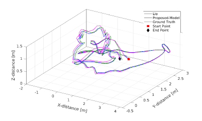
(a) Fast 1

(b) Slow 2

Figure 2: Estimated trajectories against the ground-truth trajectories

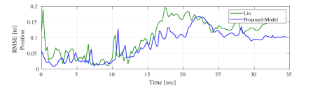
(a) RMSE on Position Error

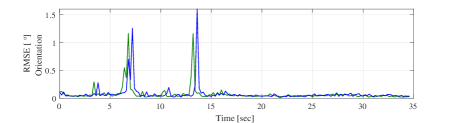
(b) RMSE on Orientation Error

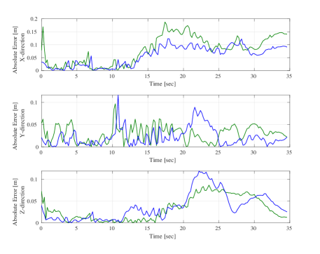
(c) Absolute Error

Figure 3: RMSE and position analysis on Fast 1 Sequence for the proposed LIO and the LIO [17]

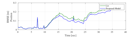
(a) RMSE on Position Error

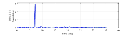
(b) RMSE on Orientation Error

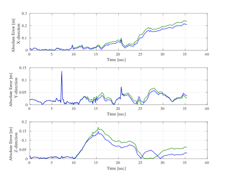
(c) Absolute Error

Figure 4: RMSE and position analysis on Slow 2 Sequence for the proposed LIO and the LIO [17]

In the case of the slow motion, the proposed algorithm outperforms the state-of-the-art one in [17] by $1.8\%$ and $13.79\%$ on Slow 1 and Slow 2 sequences, respectively. The results seem to be unexpected because the state-of-the-art motion integration model in [20, 28] outperforms the proposed motion integration model in the IMU odometry as shown in Table II. The improvement comes from the proposed IMU model which has been deployed as a tightly coupled with LiDAR factor, and from the transformation matrix (80) or (82) which is more accurate than the corresponding matrix in the state-of-the-art one. The de-skewing algorithm in [17] first computes the transformation matrix from the first point to the last point, and then linearly interpolates a transformation matrix for each point to be corrected. The interpolated transformation matrix is not accurate if the motion of the agent is not linear.

Figure 2 shows the aligned estimated trajectories against the ground-truth for Fast 1 and Slow 2 sequences. Clearly, the Fast 1 trajectory is more complicated and has many turning points than the Slow 2 trajectory. The proposed algorithm behaves well on both the trajectories. Figures 3 and 4 show the RMSE on position and orientation, and the absolute error analysis in the three dimensions on Fast 1 and Slow 2 Datasets, respectively. It shows that the proposed algorithm has a good performance in terms of the RMSE over the full trajectory. It is also observed that the difference in state estimation between the proposed algorithm and the state-of-the-art one in [17] is increased along the travelling time. Moreover, Table III shows the total travelling distance and linear velocity for each sequence.

Overall, the proposed LIO algorithm outperforms the state-of-the-art in [17] especially for complicated movements. The proposed model shows the reliability and robustness on the state estimation.

V-C Evaluation of De-skewing and LIO with Metric Maps

In this subsection, effect of metric maps to the LIO will be studied and discussed. The proposed algorithm is compared with the state-of-the-art one in [17] and the LOAM [16]. LOAM is one of the top accurate state estimation algorithms, and it shows a high accuracy estimation on the most popular dataset in the LO field, i.e., Kitti datasets [36]. This dataset has been recorded and obtained using a ground vehicle (GV). It is worth noting that the state estimation using the LOAM is done without any assistance from the IMU.

TABLE IV: Comparison of Proposed LIO Algorithm with the LIO Algorithm in [17] with Metric Maps and the LOAM in [16](RMSE On Position For Different Real Sequences With Different Motion Speeds)

	Proposed LIO with Metric Map		LIO in [17] with Metric Map				LOAM [16]
	Position		Position				Position
	RMSE	$\sigma$	RMSE	$\sigma$	Difference	Percentage	RMSE	$\sigma$	Difference	Percentage
Sequence	[cm]	[cm]	[cm]	[cm]	[cm]	[$\%$]	[cm]	[cm]	[cm]	[$\%$]
Fast 1	5.03	2.10	5.09	2.03	0.06	1.05	155.49	69.37	-	-
Fast 2	9.65	5.75	9.92	5.75	0.27	2.71	152.81	102.15	-	-
Med 1	10.94	5.32	10.94	5.24	-	-	203.78	136.82	-	-
Med 2	7.74	6.19	7.97	6.33	0.23	3.00	158.93	115.31	-	-
Slow 1	6.09	2.77	5.80	2.67	-0.29	-4.97	15.57	8.24	9.48	60.89
Slow 2	5.13	2.20	5.32	2.48	0.19	3.57	9.22	5.22	4.09	44.36

Table IV illustrates the RMSE on position of the full trajectory for the proposed algorithm, the LIO_mapping in [17], and the LOAM. The results show that the LOAM fails to estimate the state in the presence of fast or medium speed motion. There is no assistance from the IMU and the LOAM fails on these conditions. The RMSE of position for the LOAM on the Fast and Med datasets are highlighted using the green color in Table IV. The red highlight indicates that the LOAM fails to estimation the position of the robot as shown in Figure 5.

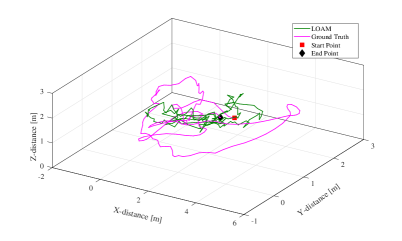
Figure 5: Estimated trajectory via the LOAM against the ground-truth one on Fast 1 Dataset

The proposed algorithm shows a superior’s performance compared to the LOAM on these conditions by $60.89\%$ on Slow 1 dataset and by $44.36\%$ on Slow 2 dataset. This is because 1) the proposed de-skewing algorithm does not assume the motion of the agent to be linear during the sweep as required by the LOAM; and 2) the proposed motion integration model is integrated with the LiDAR factor via the tightly coupled joint optimization in [17]. It should be pointed out that the accuracy of LOAM will be improved if an IMU is deployed as an additional sensor as mentioned in [23].

The results in Table IV show that the proposed algorithm and the state-of-the-art one in [17] are comparable in presence of metric maps. This is because the results highly depend on the metric map with salient features.

V-D Further Evaluation of The Proposed De-skewing Algorithm

Recently, an interesting LIO algorithm was proposed in [34]. The de-skewing algorithm in [34] is replaced by the proposed one and the implementation is on top of the open-source code of LIO-SAM and one dataset in [34]. Both GPS and loop closure are disabled to test the effectiveness of the proposed model.

One dataset in [34] was recorded in the park which is covered by vegetation using a Velodyne VLP-16 LiDAR and a MicroStrain 3DM-GX5-25 IMU mounted on UGV. The sampling rates of the LiDAR and IMU are 10 Hz and 500 Hz, respectively.

Table V shows the Root Mean Square Error (RMSE) w.r.t the ground-truth provided by GPS. The RMSE results obtained in Table V do not include the error in the z-direction or orientation errors. The reason is that the ground-truth in the park dataset does not have z-direction or orientation measurements. The results show that the proposed algorithm outperforms the state-of-the-art LIO-SAM by $11.53\%$. Figure 6 shows the estimated trajectories against the ground-truth on the park dataset, while Figures 7.(a) and 7.(b) show the RMSE on 2D position and the absolute error analysis in the two dimensions on the park dataset, respectively. It shows that the proposed algorithm has a slightly better performance and estimation regarding the RMSE over the full trajectory w.r.t the state-of-the-art one.

TABLE V: RMSE On 2D Position w.r.t GPS

	Proposed		Lio_sam [34]		Difference	Percentage	Total Distance	Linear Velocity
	RMSE	$\sigma$	RMSE	$\sigma$
Sequence	[m]	[m]	[m]	[m]	[m]	[$\%$]	[m]	[m/s]
park	25.63	11.56	28.97	13.21	3.34	11.53	656.85	1.1932

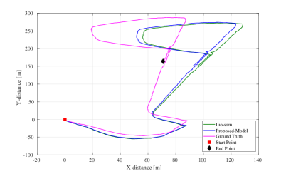
Figure 6: Estimated trajectories against the ground-truth trajectories

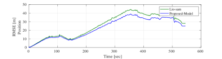
(a) RMSE on Position Error

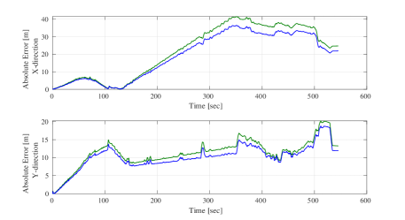
(b) Absolute Error

Figure 7: RMSE and position analysis on Park dataset

VI Conclusion Remarks

A novel piecewise linear de-skewing algorithm has been proposed for LiDAR inertial odometry (LIO) of fast moving agents using high frequency motion information provided by an inertial measurement unit (IMU). The robustness of the LIO can be enhanced by incorporating the proposed de-skewing algorithm into the LIO. Experimental results validated the performance of the proposed de-skewing algorithm. Due to its simplicity, the proposed de-skewing algorithm is practical for real world deployment.

References

- [1] J. Henawy, Z. Li, W. Y. Yau, G. Seet, and K. W. Wan, “Accurate imu preintegration using switched linear systems for autonomous systems,” in 2019 IEEE Intelligent Transportation Systems Conference (ITSC). IEEE, 2019, pp. 3839–3844.
- [2] M. Demir and K. Fujimura, “Robust localization with low-mounted multiple lidars in urban environments,” in 2019 IEEE Intelligent Transportation Systems Conference (ITSC). IEEE, 2019, pp. 3288–3293.
- [3] B. Cao, C.-N. Ritter, D. Göhring, and R. Rojas, “Accurate localization of autonomous vehicles based on pattern matching and graph-based optimization in urban environments,” in 2020 IEEE 23rd International Conference on Intelligent Transportation Systems (ITSC). IEEE, 2020, pp. 1–6.
- [4] E. Javanmardi, M. Javanmardi, Y. Gu, and S. Kamijo, “Autonomous vehicle self-localization based on probabilistic planar surface map and multi-channel lidar in urban area,” in 2017 IEEE 20th International Conference on Intelligent Transportation Systems (ITSC). IEEE, 2017, pp. 1–8.
- [5] L. J. Chen, J. Henawy, B. B. Kocer, and G. G. L. Seet, “Aerial robots on the way to underground: An experimental evaluation of vins-mono on visual-inertial odometry camera,” in 2019 International Conference on Data Mining Workshops (ICDMW). IEEE, 2019, pp. 91–96.
- [6] T. Shan and B. Englot, “Lego-loam: Lightweight and ground-optimized lidar odometry and mapping on variable terrain,” in 2018 IEEE/RSJ International Conference on Intelligent Robots and Systems (IROS). IEEE, 2018, pp. 4758–4765.
- [7] C. Le Gentil, T. Vidal-Calleja, and S. Huang, “In2lama: Inertial lidar localisation and mapping,” in 2019 International Conference on Robotics and Automation (ICRA). IEEE, 2019, pp. 6388–6394.
- [8] J. F. Chow, B. B. Kocer, J. Henawy, G. Seet, Z. Li, W. Y. Yau, and M. Pratama, “Toward underground localization: Lidar inertial odometry enabled aerial robot navigation,” arXiv preprint arXiv:1910.13085, 2019.
- [9] F. Lu and E. Milios, “Robot pose estimation in unknown environments by matching 2d range scans,” Journal of Intelligent and Robotic systems, vol. 18, no. 3, pp. 249–275, 1997.
- [10] Y. Chen and G. G. Medioni, “Object modeling by registration of multiple range images.” Image Vision Comput., vol. 10, no. 3, pp. 145–155, 1992.
- [11] P. J. Besl and N. D. McKay, “Method for registration of 3-d shapes,” in Sensor fusion IV: control paradigms and data structures, vol. 1611. International Society for Optics and Photonics, 1992, pp. 586–606.
- [12] S. Rusinkiewicz and M. Levoy, “Efficient variants of the icp algorithm,” in Proceedings Third International Conference on 3-D Digital Imaging and Modeling. IEEE, 2001, pp. 145–152.
- [13] J. Minguez, L. Montesano, and F. Lamiraux, “Metric-based iterative closest point scan matching for sensor displacement estimation,” IEEE Transactions on Robotics, vol. 22, no. 5, pp. 1047–1054, 2006.
- [14] A. Diosi and L. Kleeman, “Fast laser scan matching using polar coordinates,” The International Journal of Robotics Research, vol. 26, no. 10, pp. 1125–1153, 2007.
- [15] O. Bezet and V. Cherfaoui, “Time error correction for laser range scanner data,” in 2006 9th International Conference on Information Fusion. IEEE, 2006, pp. 1–7.
- [16] J. Zhang and S. Singh, “Loam: Lidar odometry and mapping in real-time.” in Robotics: Science and Systems, vol. 2, no. 9, 2014.
- [17] H. Ye, Y. Chen, and M. Liu, “Tightly coupled 3d lidar inertial odometry and mapping,” in 2019 International Conference on Robotics and Automation (ICRA). IEEE, 2019, pp. 3144–3150.
- [18] J. Henawy, Z. Li, W.-Y. Yau, and G. Seet, “Accurate imu factor using switched linear systems for vio,” IEEE Transactions on Industrial Electronics, vol. 68, no. 8, pp. 7199–7208, 2021.
- [19] K. Eckenhoff, P. Geneva, and G. Huang, “Closed-form preintegration methods for graph-based visual–inertial navigation,” The International Journal of Robotics Research, vol. 38, no. 5, pp. 563–586, 2019.
- [20] C. Forster, L. Carlone, F. Dellaert, and D. Scaramuzza, “On-manifold preintegration for real-time visual–inertial odometry,” IEEE Transactions on Robotics, vol. 33, no. 1, pp. 1–21, 2016.
- [21] F. Pomerleau, F. Colas, R. Siegwart, and S. Magnenat, “Comparing icp variants on real-world data sets,” Autonomous Robots, vol. 34, no. 3, pp. 133–148, 2013.
- [22] S. Hong, H. Ko, and J. Kim, “Vicp: Velocity updating iterative closest point algorithm,” in 2010 IEEE International Conference on Robotics and Automation. IEEE, 2010, pp. 1893–1898.
- [23] J. Zhang and S. Singh, “Low-drift and real-time lidar odometry and mapping,” Autonomous Robots, vol. 41, no. 2, pp. 401–416, 2017.
- [24] J. Tang, Y. Chen, X. Niu, L. Wang, L. Chen, J. Liu, C. Shi, and J. Hyyppä, “Lidar scan matching aided inertial navigation system in gnss-denied environments,” Sensors, vol. 15, no. 7, pp. 16 710–16 728, 2015.
- [25] S. Lynen, M. W. Achtelik, S. Weiss, M. Chli, and R. Siegwart, “A robust and modular multi-sensor fusion approach applied to mav navigation,” in 2013 IEEE/RSJ international conference on intelligent robots and systems. IEEE, 2013, pp. 3923–3929.
- [26] A. Soloviev, D. Bates, and F. Van Graas, “Tight coupling of laser scanner and inertial measurements for a fully autonomous relative navigation solution,” Navigation, vol. 54, no. 3, pp. 189–205, 2007.
- [27] G. Hemann, S. Singh, and M. Kaess, “Long-range gps-denied aerial inertial navigation with lidar localization,” in 2016 IEEE/RSJ International Conference on Intelligent Robots and Systems (IROS). IEEE, 2016, pp. 1659–1666.
- [28] T. Qin, P. Li, and S. Shen, “Vins-mono: A robust and versatile monocular visual-inertial state estimator,” IEEE Transactions on Robotics, vol. 34, no. 4, pp. 1004–1020, 2018.
- [29] C. Park, P. Moghadam, S. Kim, A. Elfes, C. Fookes, and S. Sridharan, “Elastic lidar fusion: Dense map-centric continuous-time slam,” in 2018 IEEE International Conference on Robotics and Automation (ICRA). IEEE, 2018, pp. 1206–1213.
- [30] C. Le Gentil, T. Vidal-Calleja, and S. Huang, “3d lidar-imu calibration based on upsampled preintegrated measurements for motion distortion correction,” in 2018 IEEE International Conference on Robotics and Automation (ICRA). IEEE, 2018, pp. 2149–2155.
- [31] F. Zhang, Matrix theory: basic results and techniques. Springer Science & Business Media, 2011.
- [32] Z. G. Li, Y. C. Soh, and C. Y. Wen, “Robust stability of a class of hybrid nonlinear systems,” IEEE Transactions on Automatic Control, vol. 46, no. 6, pp. 897–903, 2001.
- [33] Z. Li, Y. Soh, and C. Wen, Switched and impulsive systems: Analysis, design and applications. Springer Science & Business Media, 2005, vol. 313.
- [34] T. Shan, B. Englot, D. Meyers, W. Wang, C. Ratti, and D. Rus, “Lio-sam: Tightly-coupled lidar inertial odometry via smoothing and mapping,” arXiv preprint arXiv:2007.00258, 2020.
- [35] Z. Zhang and D. Scaramuzza, “A tutorial on quantitative trajectory evaluation for visual (-inertial) odometry,” in 2018 IEEE/RSJ International Conference on Intelligent Robots and Systems (IROS). IEEE, 2018, pp. 7244–7251.
- [36] A. Geiger, P. Lenz, C. Stiller, and R. Urtasun, “Vision meets robotics: The kitti dataset,” The International Journal of Robotics Research, vol. 32, no. 11, pp. 1231–1237, 2013.