Intervalley Tunneling and Crossover from the Positive to Negative Interlayer Magnetoresistance in Quasi-Two-Dimensional Dirac Fermion System with or without Mass Gap

Abstract

We theoretically investigate the interlayer magnetoresistance in quasi-two-dimensional Dirac fermion systems, where the Fermi energy is at the Dirac point. If there is an intermediate insulating layer that has an overlap with the wave functions in the Dirac fermion layers, there appears a positive magnetoresistance regime due to the intervalley tunneling. We show that the interlayer magnetoresistance can be used to find whether Dirac fermions are massive or not from the minimum in the interlayer magnetoresistance. As a specific system, we consider $\alpha$-(BEDT-TTF)₂I₃ under high pressure. We also discuss that one has to be careful in analyzing the crossover temperature from the positive to negative magnetoresistance. A simple picture is applied to the crossover in the zero temperature limit but it does not apply to the data at finite temperatures. We show that the ratio of the Fermi velocity to the scattering rate is evaluated from the zero temperature limit of the crossover temperature.

I Introduction

$\alpha$-(BEDT-TTF)₂I₃ under pressure is an organic Dirac semimetal and provides an attractive platform to investigate the physics of the Dirac fermion state.Kobayashi et al. (2004); Katayama et al. (2006); Kajita et al. (2014) The system has a quasi-two-dimensional structure consisting of alternating layers of the BEDT-TTF molecules with two-dimensional Dirac points and an iodine layer, which is insulating. (Here, BEDT-TTF is bis(ethylenedithio)tetrathiafulvalene.) Remarkably, the Fermi energy is at the Dirac point that is suitable for investigating the intrinsic properties of the Dirac fermions. Furthermore, it is possible to change the Coulomb interaction from the weak to strong coupling regimes. The quantum phase transition is investigated in the strong coupling regime, and it turns out that the system approaches the quantum critical point without creating any mass gap from the weak coupling regime.Unozawa et al. (2020); Kobayashi (2021)

The presence of the Dirac fermion spectrum is clearly demonstrated in the interlayer magnetoresistance.Tajima et al. (2009) Since the Fermi energy is at the Dirac point, the density of states vanishes at the Fermi energy in the absence of the magnetic field. By applying a magnetic field, there appears the zero energy Landau level that is absent in the conventional Landau levels of non-relativistic electrons. Because of the huge degeneracy in the zero-energy Landau level, the interlayer magnetoresistance is expected to be negative and be in inversely proportional to the applied magnetic field. The experiment is consistent with the theoretical resultOsada (2008) based on the zero energy Landau level. However, the system first exhibits a positive magnetoresistance as the applied magnetic field is increased, and then it shows a negative magnetoresistance. The magnetoresistance can be positive if there is mixing between different Landau levels.Morinari and Tohyama (2010) Although such mixing is possible when the direction of the interlayer hopping is nonvertical, the mechanism is not so convincing because the spatial translation of the Landau level wave functions upon interlayer hopping is much shorter than the magnetic length.

In this paper, we reconsider the mechanism of the positive magnetoresistance. We also consider how the interlayer resistivity is used to distinguish massless and massive Dirac fermions. We point out that there is an inter-valley interlayer hopping due to the overlaps between the molecular wave functions in BEDT-TTF layers and those in the iodine layers. We show that the inter-valley hopping clearly leads to the positive magnetoresistance under weak fields. We also investigate the effect of the mass gap in the Dirac fermion spectrum on the interlayer magnetoresistance. Recently, the effect of the spin-orbit coupling was considered in the related organic compounds.Winter et al. (2017) A possibility of the topological insulating state in $\alpha$-(BEDT-TTF)₂I₃ has been proposed.Osada (2018) We show that the interlayer magnetoresistance can be used to clarify whether there is a mass gap or not. We also describe a method to extract the ratio of the Fermi velocity to the scattering rate from the interlayer magnetoresistance measurements.

The rest of the paper is organized as follows. In Sect. II we formulate the inter-layer hopping with including the presence of the iodine layers, and show that there is an inter-valley interlayer tunneling. In Sect. III we derive the formula for the interlayer conductivity under magnetic fields with and without the mass gap. In Sect. IV we present the result and discuss how one can distinguish the massless and massive cases. We also discuss how the interlayer magnetoresistance experiment is used to estimate the ratio of the Fermi velocity to the scattering rate of the Dirac fermions. Section V is devoted to conclusion.

II The model for the interlayer tunneling

In this section we establish that there is an effective inter-valley electron hopping between BEDT-TTF layers by explicitly taking into account the presence of the iodine layers in between. As revealed by the first principles calculation,Kino and Miyazaki (2006) there is mixing between the BEDT-TTF and I${}_{3}^{-}$ molecules. Therefore, electrons do not hop directly between adjacent BEDT-TTF layers. They hop from a BEDT-TTF layer to the adjacent iodine layer, and then hop to another BEDT-TTF layer. Because of this intermediate process, the inter-valley hopping is possible. If we denote the hopping amplitude between BEDT-TTF and iodine layers by $t^{\prime}$, then we obtain the effective hopping $t_{c}$ between adjacent BEDT-TTF layers by applying the second order perturbation theory with respect to $t^{\prime}$. The result is,

$${t_{c}}=-\frac{{2{{t^{\prime}}^{2}}}}{{{U_{p}}+{\varepsilon_{p}}}}-\frac{{{{t^{\prime}}^{2}}}}{{{U_{p}}-U+{\varepsilon_{p}}}}$$ (1)

where $U_{p}$ and $U$ are the onsite Coulomb repulsions at the iodine and BEDT-TTF layers, respectively. $\varepsilon_{p}$ is the energy of the single-electron at the iodine layer. The LUMO+1 and LUMO+2, where LUMO is the lowest-unoccupied-molecular-orbital, are around 1eV above the Fermi energy and consist of I${}_{3}^{-}$ molecules.Kino and Miyazaki (2006) So, $\varepsilon_{p}\sim 1$eV.

We emphasize that $t_{c}$ is not the direct hopping amplitude of electrons between BEDT-TTF layers. If $t_{c}$ were the direct hopping amplitude, then there would be no tunneling between different valleys in the Dirac fermion phase. Since $t_{c}$ is related to $t^{\prime}$ that is the hopping amplitude between BEDT-TTF and I${}_{3}^{-}$ molecules, the tunneling is not restricted to the same valleys but there is also the inter-valley tunneling.

Now we present the effective interlayer tunneling term between BEDT-TTF layers in the Dirac fermion phase of $\alpha$-(BEDT-TTF)₂I₃ that is used to derive the formula for the interlayer conductivity under magnetic field. From the consideration above, the inter-layer hopping includes the inter-valley hopping. Our model Hamiltonian for the interlayer tunneling is given by

$${H_{c}}={t_{c}}\sum\limits_{n,n^{\prime},\tau,\tau^{\prime},k,\sigma,\ell}{\left({{M_{n\tau,n^{\prime}\tau^{\prime}}}c_{n\tau k\sigma,\ell+1}^{\dagger}{c_{n^{\prime}\tau^{\prime}k\sigma,\ell}}+H.c.}\right)}$$ (2)

Here, the operator ${c_{n\tau k\sigma,\ell}^{\dagger}}$ is the creation operator for a Dirac fermion with the Landau level index $n$, valley index $\tau$, the wave number $k$, and spin $\sigma$ in the $\ell$-th layer. A summary of the Dirac fermion Landau levels is given in Appendix A. We note that $M_{n\tau,n^{\prime}\tau^{\prime}}$ is a function of $k$, $k^{\prime}$, $\tau$, and $\tau^{\prime}$, in general but here we assume $k^{\prime}=k$ for simplicity. $M_{n\tau,n^{\prime}\tau^{\prime}}$ are the matrix elements between the Landau level $n$ at valley $\tau$ and the Landau level $n^{\prime}$ at valley $\tau^{\prime}$ that is given by

$${M_{n\tau,n^{\prime}\tau^{\prime}}}=\left\langle{{n,\tau}}\mathrel{\left|{\vphantom{{n,\tau}{n^{\prime},\tau^{\prime}}}}\right.\kern-1.2pt}{{n^{\prime},\tau^{\prime}}}\right\rangle,$$ (3)

where $\left|{n,\tau}\right\rangle$ is defined in Appendix A.

III Interlayer magnetoresistance formula

In this section we derive the formula for the interlayer conductivity based on Eq. (2). We assume that $t_{c}$ is much smaller than the intralayer scattering rate, $\Gamma$. Under this condition the interlayer conductivity is proportional to the tunneling rate between two adjacent layersMcKenzie and Moses (1998); Moses and McKenzie (1999) labeled by layer-1 and -2. The tunneling Hamiltonian between these two layers is given by

$${H_{12}}={t_{c}}\sum\limits_{\alpha,\alpha^{\prime}}{\left({{M_{\alpha^{\prime}\alpha}}c_{\alpha^{\prime}2}^{\dagger}{c_{\alpha 1}}+{M_{\alpha\alpha^{\prime}}}c_{\alpha 1}^{\dagger}{c_{\alpha^{\prime}2}}}\right)},$$ (4)

where we denote a set of parameters, $n,\tau,k,\sigma$ by a single Greek symbol, $\alpha$, to simplify the notation. Since the spin is conserved upon the interlayer tunneling, we set

$${M_{\alpha\alpha^{\prime}}}={\delta_{k,k^{\prime}}}{\delta_{\sigma,\sigma^{\prime}}}{M_{n\tau,n^{\prime}\tau^{\prime}}}.$$ (5)

The interlayer current $I$ produced by an applied voltage $V$ across the layers is calculated as in a metal-insulator-metal junction.Mahan (1990) The current $I$ is associated with the change of the number of particles in layer-1,

$${N_{1}}=\sum\limits_{\alpha}{c_{\alpha 1}^{\dagger}{c_{\alpha 1}}}.$$ (6)

Under the applied voltage $V$, the chemical potential difference between the layers is ${\mu_{1}}-{\mu_{2}}=eV$, where $\mu_{1}$ and $\mu_{2}$ denote the chemical potentials at each layer. Applying the Kubo formula, we obtain

$$I\left(t\right) = -\frac{{et_{c}^{2}}}{{{\hbar^{2}}}}\int_{-\infty}^{\infty}{dt^{\prime}}\theta\left({t-t^{\prime}}\right)\left[{e^{-\frac{i}{\hbar}\left({{\mu_{2}}-{\mu_{1}}}\right)\left({t-t^{\prime}}\right)}}\right.$$ (7)

$$\left.\times\left\langle{\left[{A\left(t\right),{A^{\dagger}}\left({t^{\prime}}\right)}\right]}\right\rangle\right.$$

$$\left.-{e^{+\frac{i}{\hbar}\left({{\mu_{2}}-{\mu_{1}}}\right)\left({t-t^{\prime}}\right)}}\left\langle{\left[{{A^{\dagger}}\left(t\right),A\left({t^{\prime}}\right)}\right]}\right\rangle\right],$$

where

$$A=\sum\limits_{\alpha,\alpha^{\prime}}{{M_{\alpha^{\prime}\alpha}}c_{\alpha^{\prime}2}^{\dagger}{c_{\alpha 1}}},$$ (8)

$${A^{\dagger}}=\sum\limits_{\alpha,\alpha^{\prime}}{{M_{\alpha\alpha^{\prime}}}c_{\alpha 1}^{\dagger}{c_{\alpha^{\prime}2}}},$$ (9)

and

$$A\left(t\right)=\exp\left({\frac{i}{\hbar}Kt}\right)A\exp\left({-\frac{i}{\hbar}Kt}\right),$$ (10)

with $K=\sum\limits_{\alpha,j=1,2}{\left({{\varepsilon_{\alpha}}-\mu}\right)c_{\alpha j}^{\dagger}{c_{\alpha j}}}$. Here, $\mu$ is the chemical potential in the absence of the voltage drop. $\varepsilon_{\alpha}$ denotes the energy of the single-particle state, $\alpha$, whose Landau energy part is given in Appendix A and the Zeeman energy, $\mu_{\rm B}B$, is included. (The spin $g$-factor is set to 2.)

Introducing the retarded and advanced Green’s functions,

$${D_{R}}\left({t-t^{\prime}}\right)=-\frac{i}{\hbar}\theta\left({t-t^{\prime}}\right)\left\langle{\left[{A\left(t\right),{A^{\dagger}}\left({t^{\prime}}\right)}\right]}\right\rangle,$$ (11)

$${D_{A}}\left({t-t^{\prime}}\right)=+\frac{i}{\hbar}\theta\left({t^{\prime}-t}\right)\left\langle{\left[{A\left(t\right),{A^{\dagger}}\left({t^{\prime}}\right)}\right]}\right\rangle,$$ (12)

and their Fourier transforms $D_{R}(\omega)$ and $D_{A}(\omega)$, Eq. (7) is rewritten as

$$I=\frac{{ie}}{\hbar}t_{c}^{2}\left[{{D_{R}}\left({eV/\hbar}\right)-{D_{A}}\left({eV/\hbar}\right)}\right].$$ (13)

${D_{R}}\left(\omega\right)$ and ${D_{A}}\left(\omega\right)$ are obtained from the Matsubara Green’s function ${D_{M}}\left(i\omega_{n}\right)$ by the analytic continuation. ${D_{M}}\left(i\omega_{n}\right)$ is given by

$${D_{M}}\left({i{\Omega_{n}}}\right)=\frac{1}{\beta}\sum\limits_{\alpha,\alpha^{\prime}}{{{\left|{{M_{\alpha^{\prime}\alpha}}}\right|}^{2}}}\sum\limits_{i{\omega_{n}}}{{G_{\alpha 1}}\left({i{\omega_{n}}+i{\Omega_{n}}}\right){G_{\alpha 2}}\left({i{\omega_{n}}}\right)},$$ (14)

where $\beta=1/(k_{\rm B}T)$ with $k_{\rm B}$ the Boltzmann constant. $\omega_{n}$ and $\Omega_{n}$ are fermionic and bosonic Matsubara frequencies, respectively. The single-body Green’s function is given by

$${G_{\alpha j}}\left({i{\omega_{n}}}\right)=\int_{0}^{\beta}{d\tau}{e^{i{\omega_{n}}\tau}}{G_{\alpha j}}\left(\tau\right),$$ (15)

with

$${G_{\alpha j}}\left(\tau\right)=-\left\langle{{T_{\tau}}{c_{\alpha j}}\left(\tau\right)c_{\alpha j}^{\dagger}\left(0\right)}\right\rangle.$$ (16)

Here, $T_{\tau}$ is the imaginary-time ordering operator and ${c_{\alpha j}}\left(\tau\right)=\exp\left({\tau K}\right){c_{\alpha j}}\exp\left({-\tau K}\right)$.

Introducing the spectral representation of the single-particle Green’s function, we carry out the summation over $i\omega_{n}$. After the analytic continuation, we obtain

$${\mathop{\rm Im}\nolimits}{D_{R}}\left(\omega\right) = \pi\sum\limits_{\alpha,\alpha^{\prime}}{{{\left|{{M_{\alpha^{\prime}\alpha}}}\right|}^{2}}}\int_{-\infty}^{\infty}{d{\omega_{1}}}\int_{-\infty}^{\infty}{d{\omega_{2}}}$$ (17)

$$\times\left[{f\left({{\omega_{1}}}\right)-f\left({{\omega_{2}}}\right)}\right]\delta\left({\hbar\omega-{\omega_{1}}+{\omega_{2}}}\right)$$

$$\times{A_{\alpha 1}}\left({{\omega_{1}}}\right){A_{\alpha^{\prime}2}}\left({{\omega_{2}}}\right),$$

with $f\left(\varepsilon\right)=1/\left({\exp\left({\beta\varepsilon}\right)+1}\right)$ the Fermi-Dirac distribution function. Here, ${A_{\alpha j}}\left(\omega\right)$ is given by

$${A_{\alpha j}}\left(\omega\right)=-\frac{1}{\pi}{\mathop{\rm Im}\nolimits}{G_{\alpha j}}\left({\omega+i\delta}\right).$$ (18)

From Eq. (13), the interlayer conductivity is

$${\sigma_{zz}} = \frac{{2\pi{e^{2}}t_{c}^{2}{a_{c}}}}{{\hbar{L^{2}}}}\sum\limits_{\alpha,\alpha^{\prime}}{{{\left|{{M_{\alpha^{\prime}\alpha}}}\right|}^{2}}}\int_{-\infty}^{\infty}{d\omega}\left({-\frac{{\partial f}}{{\partial\omega}}}\right)$$ (19)

$$\times{A_{\alpha 1}}\left(\omega\right){A_{\alpha^{\prime}2}}\left(\omega\right)$$

with $a_{c}$ the $c$-axis lattice constant and $L^{2}$ the area of the layer. Carrying out the $k$-summation, we obtain

$${\sigma_{zz}} = \frac{{{e^{3}}t_{c}^{2}{a_{c}}}}{{{\hbar^{2}}}}B\sum\limits_{n,n^{\prime},\tau,\tau^{\prime},\sigma}{{{\left|{{M_{n\tau,n^{\prime}\tau^{\prime}}}}\right|}^{2}}}\int_{-\infty}^{\infty}{d\omega}$$ (20)

$$\times\left({-\frac{{\partial f}}{{\partial\omega}}}\right){A_{n\tau\sigma}}\left(\omega\right){A_{n^{\prime}\tau^{\prime}\sigma}}\left(\omega\right).$$

Note that we omit the indices for layer-1 and -2 hereafter because the spectral function $A_{n\tau\sigma}$ has the same functional form. The explicit forms of $M_{n\tau,n^{\prime}\tau^{\prime}}$ are given in Appendix B.

A convenient form of Eq. (20) is obtained by dividing it by ${\sigma_{0}}=\left({{e^{2}}/\hbar{a_{c}}}\right){\left({{t_{c}}/\Gamma}\right)^{2}}$. That is,

$$\frac{{{\sigma_{zz}}}}{{{\sigma_{0}}}} = \frac{e}{\hbar}a_{c}^{2}B\times{\Gamma^{2}}\sum\limits_{n,n^{\prime},\tau,\tau^{\prime},\sigma}{{{\left|{{M_{n\tau,n^{\prime}\tau^{\prime}}}}\right|}^{2}}}$$ (21)

$$\times\int_{-\infty}^{\infty}{d\omega}\left({-\frac{{\partial f}}{{\partial\omega}}}\right){A_{n\tau\sigma 1}}\left(\omega\right){A_{n^{\prime}\tau^{\prime}\sigma 2}}\left(\omega\right).$$

If we measure the magnetic field $B$ in units of Tesla and taking ${a_{c}}=1.7488\times{10^{-9}}\,{\rm{m}}$,Bender et al. (1984) we obtain $ea_{c}^{2}B/\hbar=4.646\times{10^{-3}}\times B\left[{\rm{T}}\right]$.

IV Results

IV.1 Massless Dirac fermions

Now we show the results for the massless Dirac fermion case. As will be shown below we clearly see the crossover from the positive to negative magnetoresistance regimes. Figure 1 shows the temperature dependence of the interlayer resistivity for different magnetic fields. Hereafter, we take $v_{F}=5\times 10^{4}$ m/s and $\Gamma=1$ K unless otherwise stated. We plot the interlayer resistivity at $B=0$ as well, whose formula is given in Appendix C. The steep rise close to zero temperature is associated with the energy gap created by the Zeeman energy, which is of no importance. Apart from that peak, we clearly see the crossover from the positive to negative magnetoresistance regimes. The interlayer resistivity shows a peak at the crossover temperature, $T_{\rm max}$. For example $T_{\rm max}\sim 10$ K for $B=3$ T. In the positive magnetoresistance regime, $T<T_{\rm max}$, the inter-Landau level mixing occurs, and this dominates over the increase of the conductivity due to the Landau level degeneracy, which is proportional $B$. This Landau level mixing arises from the intervalley scattering upon the interlayer tunneling. We note that at high-temperatures the resistivity approaches to the $B=0$ value. In order to confirm this behavior, we need to carry out the Landau-level sum with a sufficient number of Landau levels because of the factor associated with the derivative of the Fermi-Dirac function that has a broad peak at high temperatures.

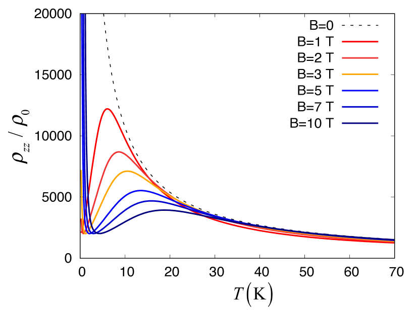
Figure 1: (Color online) The interlayer resistivity as a function of temperature for different magnetic fields with $v_{F}=5\times 10^{4}$ m/s and $\Gamma=1$ K. The dashed line is the interlayer resistivity at $B=0$. Here, ${\rho_{0}}=1/\sigma_{0}$. There is crossover from the positive magnetoresistance at low temperatures to the negative magnetoresistance at high temperatures. The Landau-level sum is taken over $-n_{\rm max}\leq n\leq n_{\rm max}$ with $n_{\rm max}=300$.

Here, we comment on the temperature dependence of $\Gamma$. In this paper we assume a constant $\Gamma$. In the experiment reported in Ref. Sugawara et al., 2010, the temperature dependence of the interlayer magnetoresistance was shown for different magnetic fields. It is possible to compute the interlayer magnetoresistance theoretically from the results above. However, the temperature dependence of the interlayer resistivity at $B=0$ in Ref. Sugawara et al., 2010 shows a broad dip that is presumably associated with the temperature dependence of $\Gamma$. The theoretical results above assumed a constant $\Gamma$. So, we need to include its temperature dependence to quantitatively explain the experiment. This point will be investigated in the future publication.

Before analyzing the magnetic field dependence of $T_{\rm max}$, we discuss the magnetic field dependence of the interlayer resistivity for different temperatures shown in Fig. 2. We also find the crossover from the positive to negative magnetoresistance regimes. There is a peak associated with this behavior. We would like to emphasize that the peaks appear both in Figs. 1 and 2. This is because the physical origin of the peaks are the same. It was argued in Ref. Yoshimura et al., 2021 that the positive magnetoresistance was possible if the Dirac fermions were massive. However, the positive magnetoresistance region is absent in the magnetic field dependence of the interlayer resistivity if one neglects the effect of the mixing between the Landau levels. Since the origin of the positive magnetoresistance is the same, just assuming the mass gap for the Dirac fermion spectrum is not enough to explain the experiment.

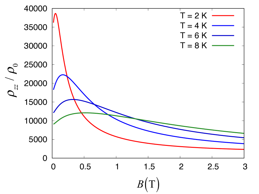
Figure 2: (Color online) The interlayer resistivity as a function of $B$ for different temperatures. There is crossover from the positive magnetoresistance at low fields to the negative magnetoresistance at high fields. The physical origin of this crossover is the same as that observed in the temperature dependence of $\rho_{zz}$ (Fig. 1).

Now we discuss $T_{\rm max}$ for different magnetic fields, and we resolve some confusing situation about its interpretation. Figure 3 shows the magnetic field dependence of $T_{\rm max}$. Roughly speaking $T_{\rm max}$ appears to be proportional to $\sqrt{B}$. One can understand this behavior as the result of the Landau level mixing. Since the Landau levels are not evenly spaced for the Dirac fermion system and the largest energy gap is that between the zero and first Landau levels, the Landau level mixing occurs when this gap is equal to $\Gamma$. If the Landau level broadening associated with $\Gamma$ is larger than the temperature effect, we may expect $T_{\rm max}\propto\sqrt{B}$ because the first Landau level energy is proportional to $\sqrt{B}$. However, one must be careful that this interpretation applies to the temperature range, $T\ll\Gamma/k_{\rm B}$. At finite temperatures it gives us just a qualitative picture. The point is that the temperature effect is not simple because that comes from the integration of the function multiplied by the derivative of the Fermi-Dirac function over the whole range of the Landau levels. In Ref. Sugawara et al., 2010, $T_{\rm max}$ is analyzed using a formula ${k_{\rm{B}}}{T_{\max}}=c\left({v\sqrt{2e\hbar B}-g{\mu_{B}}B}\right)$, with $c$ and $v$ being fit parameters. $g=2$ is the $g$-factor and $\mu_{B}$ is the Bohr magneton. The experiment was in good agreement with this formula with $c=0.93$ and $v=2.4\times 10^{4}$ m/s. However, this result requires close attention. Although $c\sim 1$, the value of $v$, which must correspond to the Fermi velocity, is almost one-half of the Fermi velocity determined from the Shubnikov-de Haas oscillation.Unozawa et al. (2020) Therefore, the simple picture above is not applicable. Meanwhile, it was argued that the Dirac fermions were massive in Ref. Yoshimura et al., 2021 based on a similar analysis. But from the observation above one is not able to conclude whether the Dirac fermions are massive or not from the finite temperature data.

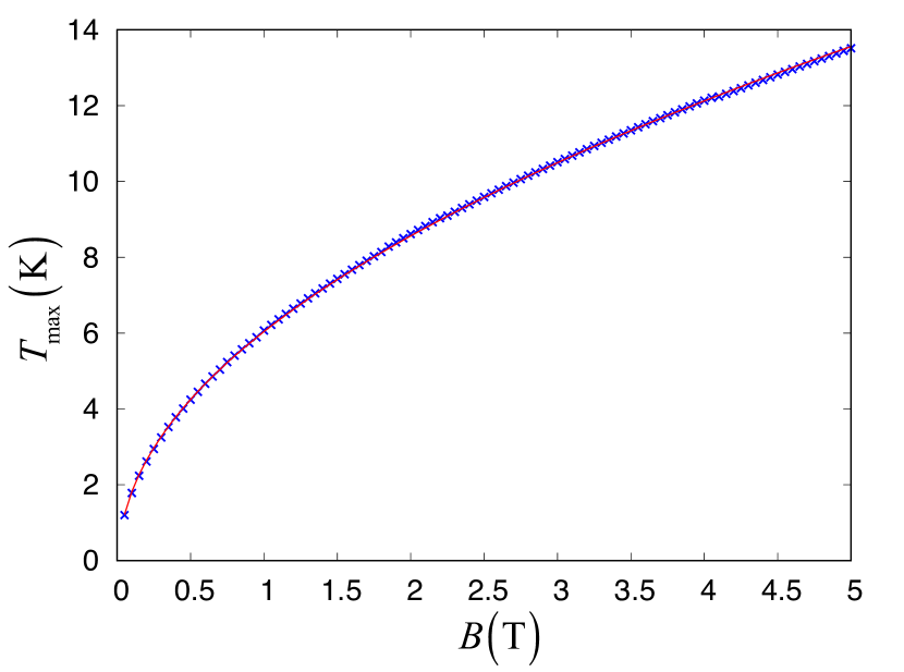
Figure 3: (Color online) The crosses show $T_{\rm max}$ as a function of $B$. The solid line is a fit to a phenomenological formula, ${T_{\max}}=C\sqrt{B-{B_{0}}}$, where $C$ and $B_{0}$ are fit parameters. From the fit we find $C=6.07$ K T^-1/2 and $B_{0}=1.0\times 10^{-2}$ T. Note that we need more careful analysis to estimate the $B_{0}$ value as discussed in the main text.

Although it is not justified to extract information about the Dirac fermion parameters from the finite temperature data, it is possible to estimate $v_{F}/\Gamma$ from the critical value of $B=B_{0}$ that is obtained by taking $T_{\rm max}\to 0$. An analysis of $T_{\rm max}$ at small magnetic fields is shown in Fig. 4. We find $B=B_{0}=2.5\times 10^{-3}$ T for the case of $v=5\times 10^{4}$ m/s and $\Gamma=1$ K. From the value of $B_{0}$ we are able to evaluate $v_{F}/\Gamma$. When the first Landau level energy is equal to $\Gamma$, we obtain

$$\frac{{{v_{F}}}}{\Gamma}=\frac{1}{{\sqrt{2\hbar eB}}}.$$ (22)

If we denote the Fermi velocity by ${v^{\prime}_{F}}$ evaluated from this formula, assuming $B=B_{0}=2.5\times 10^{-3}$ T and $\Gamma=1$ K, we find ${v^{\prime}_{F}}=0.95\times{v_{F}}$. The same analysis for $\Gamma=3$K leads to $B_{0}=2.3\times 10^{-2}$ T and ${v^{\prime}_{F}}=0.94\times{v_{F}}$. Since $v^{\prime}_{F}/v_{F}$ is very close to 1, the value of $B_{0}$ can be used to evaluate $v_{F}/\Gamma$.

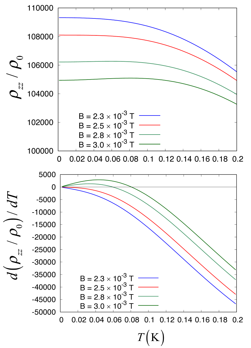
Figure 4: (Color online) The upper panel shows $\rho_{zz}/\rho_{0}$ as a function of $T$ for different magnetic fields. There are peaks for $B>2.5\times 10^{-3}$ T but no peaks for $B<2.5\times 10^{-3}$ T. This behavior becomes clearer by taking the derivative of $\rho_{zz}$ with respect to $T$ as shown in the lower panel.

IV.2 Massive Dirac fermions

Since $\alpha$-(BEDT-TTF)₂I₃ consists of light atoms, the spin-orbit coupling is considered to be very small. However, its value is estimated to be 1-2 meV based on the density functional theory.Winter et al. (2017) So, one may expect that massless Dirac fermions become massive due to the presence of the spin-orbit coupling.Osada (2018) Since the Fermi energy is at the Dirac point in $\alpha$-(BEDT-TTF)₂I₃, the mass gap affects the density of states at the Fermi energy. The energy spectrum of the massive Dirac fermions is schematically shown in Fig. 5. In the massless case, the negative magnetoresistance is associated with the appearance of the zero energy Landau levels at the Fermi energy. Meanwhile, this effect is suppressed for the massive case because the zero energy Landau level is located at $\pm m$ for the massive case. Under magnetic fields, we also need to take into account the Zeeman energy, which is not shown in Fig. 5. In the following we discuss the effect of the mass gap on the interlayer resistivity under magnetic field.

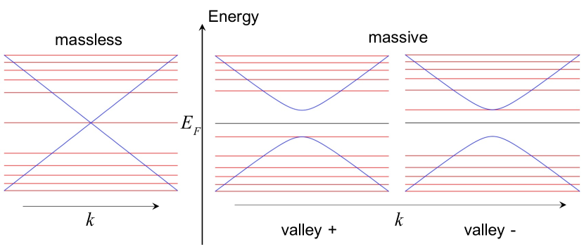
Figure 5: The energy dispersion of the massless case and the massive case. The Fermi energy is at the Dirac point. The horizontal lines are the Landau level energies. The zero energy Landau level is at $-m$ or $m$ for the massive case. (The Zeeman energy is not included here for simplicity.)

From the temperature dependence of the interlayer resistivity for different masses, we find that the positive magnetoresistance region decreases as the mass increases, and finally disappear as shown in Fig. 6. The critical mass value depends on $B$. If the Dirac fermions are massive, the positive magnetoresistance region disappears at sufficiently low magnetic fields.

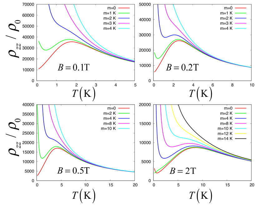
Figure 6: (Color online) The interlayer resistivity as a function of temperature for different masses. From left top to right bottom, the magnetic field is $B=0.1,0.2,0.5,2$T.

The effect of the mass term is clearly seen at the minimum of the interlayer resistivity. Figure 7 shows the magnetic field dependence of the interlayer resistivity for different masses in the magnetic field range where the minimum is seen. For the massless case the minimum is located where $\Gamma$ is equal to the Zeeman energy.Osada (2008) However, for massive cases, the minimum occurs at $\mu_{\rm B}B\simeq m$. Thus, one can find the upper limit for the mass term of the Dirac fermion system from the minimum of the interlayer resistivity. The massless case might appear different from Fig. 2. But we note that the temperature is 0.2 K and is much lower than Fig. 2. We also note that the minimum at $T=2K$ is located $B\sim 4$ T that is outside of the magnetic field range of Fig. 2.

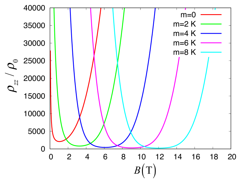
Figure 7: (Color online) The interlayer resistivity as a function of the magnetic field for different masses at $T=0.2$K. The value of the magnetic field at the resistivity minimum increases as the mass increases.

V Conclusion

To conclude, we have investigated the interlayer resistivity under magnetic field with including the intervalley scattering upon the interlayer tunneling. The intervalley scattering occurs because of the presence of the insulating layers. The formula for the interlayer resistivity has been given under magnetic field and for the case of zero-magnetic field. From the numerical calculations it is clearly seen that there is a crossover from the positive to negative magnetoresistance regimes. We have argued that the ratio of the Fermi velocity to the scattering rate, $v_{F}/\Gamma$, can be estimated from the extrapolation of $B_{0}$ at finite temperatures to zero temperature. The magnetic field dependence of the peaks observed in the temperature dependence of the interlayer resistivity is roughly proportional to $\sqrt{B}$. However, one has to be careful about extracting information about the Dirac fermion parameters from this kind of analysis because the temperature effect is not simple. As for the possibility of the mass gap in the Dirac fermion spectrum, we have pointed out that the mass value can be estimated from the minimum of the interlayer resistivity as a function of the magnetic field.

Appendix A Dirac Fermions in a Magnetic Field

In this appendix we briefly review the Dirac fermion Landau levels with including a mass gap. We consider Dirac fermions with the Fermi velocity $v_{F}$ and the mass gap $m$ at valley $\tau=+$ under magnetic field $B$, which is directed perpendicular to the layer of the Dirac fermions. The Hamiltonian is given by

$${H_{+}}=v_{F}\left({\hbar{{\widehat{k}}_{x}}+e{A_{x}}}\right){\sigma_{1}}+v_{F}\left({\hbar{{\widehat{k}}_{y}}+e{A_{y}}}\right){\sigma_{2}}+m{\sigma_{3}}.$$ (23)

Here, ${\widehat{k}_{x}}=-i{\partial_{x}}$ and ${\widehat{k}_{y}}=-i{\partial_{y}}$. $\sigma_{1}$, $\sigma_{2}$, and $\sigma_{3}$ are Pauli matrices. We use the Landau gauge, ${\bm{A}}=\left({-By,0}\right)$.

The Landau level energy is given by

$${\varepsilon_{n,+}}=\frac{{\sqrt{2}\hbar v_{F}}}{\ell}{\mathop{\rm sgn}}\left(n\right)\sqrt{\left|n\right|+{{\widetilde{m}}^{2}}},$$ (24)

for $n\neq 0$ and

$${\varepsilon_{0,+}}=-m.$$ (25)

Here, $\ell=\sqrt{\hbar/\left({eB}\right)}$ is the magnetic length, $n$ is an integer, and $\widetilde{m}=m/\left({\sqrt{2}\hbar v_{F}/\ell}\right)$. Denoting the Landau level states by $\left|{n,+}\right\rangle$, we obtain

$$\left|{0,+}\right\rangle=\left({\begin{array}[]{*{20}{c}}0\\ {\left|0\right\rangle}\end{array}}\right),$$ (26)

$$\left|{n,+}\right\rangle={C_{n}}\left({\begin{array}[]{*{20}{c}}{\left({\sqrt{n+{{\widetilde{m}}^{2}}}+{\widetilde{m}}}\right)\left|{n-1}\right\rangle}\\ {-\sqrt{n}\left|n\right\rangle}\end{array}}\right),$$ (27)

for $n>0$, and

$$\left|{n,+}\right\rangle={C_{n}}\left({\begin{array}[]{*{20}{c}}{\sqrt{\left|n\right|}\left|{\left|n\right|-1}\right\rangle}\\ {\left({\sqrt{\left|n\right|+{{\widetilde{m}}^{2}}}+{\widetilde{m}}}\right)\left|{\left|n\right|}\right\rangle}\end{array}}\right)$$ (28)

for $n<0$. Here, $\left|{\left|n\right|}\right\rangle$ are the harmonic oscillator eigenstates and

$${C_{n}}=\frac{1}{{\sqrt{2\sqrt{\left|n\right|+{{\widetilde{m}}^{2}}}\left({\sqrt{\left|n\right|+{{\widetilde{m}}^{2}}}+{\widetilde{m}}}\right)}}}.$$ (29)

The Landau levels at another valley, $\tau=-$, are obtained by making use of the transformation,

$${H_{-}}\left({\bm{k}}\right)=v_{F}\left({-\hbar{k_{x}}{\sigma_{1}}+\hbar{k_{y}}{\sigma_{2}}}+m{\sigma_{3}}\right)={\sigma_{2}}{H_{+}}\left({\bm{k}}\right){\sigma_{2}}.$$ (30)

The Landau level energies are

$${\varepsilon_{n,-}}={\varepsilon_{n,+}},$$ (31)

for $n\neq 0$ and

$${\varepsilon_{0,-}}=m.$$ (32)

The Landau level states are

$$\left|{0,-}\right\rangle=\left({\begin{array}[]{*{20}{c}}{\left|0\right\rangle}\\ 0\end{array}}\right),$$ (33)

$$\left|{n,-}\right\rangle={C_{n}}\left({\begin{array}[]{*{20}{c}}{\left({\sqrt{n+{{\widetilde{m}}^{2}}}+\widetilde{m}}\right)\left|n\right\rangle}\\ {-\sqrt{n}\left|{n-1}\right\rangle}\end{array}}\right),$$ (34)

for $n>0$ and

$$\left|{n,-}\right\rangle={C_{n}}\left({\begin{array}[]{*{20}{c}}{\sqrt{\left|n\right|}\left|{\left|n\right|}\right\rangle}\\ {\left({\sqrt{\left|n\right|+{{\widetilde{m}}^{2}}}+\widetilde{m}}\right)\left|{\left|n\right|-1}\right\rangle}\end{array}}\right),$$ (35)

for $n<0$.

Appendix B The Matrix Elements

The matrix elements $M_{n\tau,n^{\prime}\tau^{\prime}}$ are computed as follows. For the intravalley tunneling, we simply obtain

$${M_{n\tau,n^{\prime}\tau}}={\delta_{n,n^{\prime}}}.$$ (36)

In order to describe the intervalley tunneling, we define

$${A_{n}}={C_{n}}\left({\sqrt{n+{{\widetilde{m}}^{2}}}+{\widetilde{m}}}\right),$$ (37)

and

$${B_{n}}={C_{n}}\sqrt{n}.$$ (38)

In the following, $n$ and $n^{\prime}$ denote non-negative integers. In terms of $A_{n}$ and $B_{n}$, we find

$$\left\langle{{0,+}}\mathrel{\left|{\vphantom{{0,+}{0,-}}}\right.\kern-1.2pt}{{0,-}}\right\rangle = 0,$$

$$\left\langle{{0,+}}\mathrel{\left|{\vphantom{{0,+}{n,-}}}\right.\kern-1.2pt}{{n,-}}\right\rangle = -{B_{1}}{\delta_{n,1}},$$

$$\left\langle{{0,+}}\mathrel{\left|{\vphantom{{0,+}{-n,-}}}\right.\kern-1.2pt}{{-n,-}}\right\rangle = {A_{1}}{\delta_{n,1}},$$

$$\left\langle{{n,+}}\mathrel{\left|{\vphantom{{n,+}{0,-}}}\right.\kern-1.2pt}{{0,-}}\right\rangle = {A_{1}}{\delta_{n,1}},$$

$$\left\langle{{n,+}}\mathrel{\left|{\vphantom{{n,+}{n^{\prime},-}}}\right.\kern-1.2pt}{{n^{\prime},-}}\right\rangle = {\delta_{n,n^{\prime}+1}}{A_{n^{\prime}+1}}{A_{n^{\prime}}}+{\delta_{n^{\prime},n+1}}{B_{n}}{B_{n+1}},$$

$$\left\langle{{n,+}}\mathrel{\left|{\vphantom{{n,+}{-n^{\prime},-}}}\right.\kern-1.2pt}{{-n^{\prime},-}}\right\rangle = {\delta_{n,n^{\prime}+1}}{A_{n^{\prime}+1}}{B_{n^{\prime}}}-{\delta_{n^{\prime},n+1}}{B_{n}}{A_{n+1}},$$

$$\left\langle{{-n,+}}\mathrel{\left|{\vphantom{{-n,+}{0,-}}}\right.\kern-1.2pt}{{0,-}}\right\rangle = {B_{1}}{\delta_{n,1}},$$

$$\left\langle{{-n,+}}\mathrel{\left|{\vphantom{{-n,+}{n^{\prime},-}}}\right.\kern-1.2pt}{{n^{\prime},-}}\right\rangle = {B_{n^{\prime}+1}}{A_{n^{\prime}}}{\delta_{n,n^{\prime}+1}}-{A_{n}}{B_{n+1}}{\delta_{n^{\prime},n+1}},$$

$$\left\langle{{-n,+}}\mathrel{\left|{\vphantom{{-n,+}{-n^{\prime},-}}}\right.\kern-1.2pt}{{-n^{\prime},-}}\right\rangle = {B_{n^{\prime}+1}}{B_{n^{\prime}}}{\delta_{n,n^{\prime}+1}}+{A_{n}}{A_{n+1}}{\delta_{n^{\prime},n+1}}.$$

Appendix C Interlayer Conductivity in the Absence of Magnetic Field

In this appendix we compute the interlayer conductivity in the absence of the magnetic field. We can use Eq. (19) with taking $\alpha=\left({{\bm{k}},\tau,\sigma}\right)$ and $\alpha^{\prime}=\left({{\bm{k}}^{\prime},\tau^{\prime},\sigma^{\prime}}\right)$. For $M_{\alpha^{\prime}\alpha}$, we assume

$${M_{\left({{\bm{k^{\prime}}},\tau^{\prime},\sigma^{\prime}}\right),\left({{\bm{k}},\tau,\sigma}\right)}}={\delta_{\sigma^{\prime},\sigma}}{\delta_{{\bm{k^{\prime}}},{\bm{k}}}}.$$ (40)

Note that the intervalley scattering is included. There is no spin flip upon interlayer tunneling.

The ${\bm{k}}$-summation is converted into the integral:

$${\sigma_{zz}} = \frac{{4\pi{e^{2}}t_{c}^{2}{a_{c}}}}{\hbar}\int{\frac{{{d^{2}}{\bm{k}}}}{{{{\left({2\pi}\right)}^{2}}}}}\sum\limits_{s,s^{\prime}=\pm}\int_{-\infty}^{\infty}{d\omega}\left({-\frac{{\partial f}}{{\partial\omega}}}\right)$$ (41)

$$\times{A_{{\bm{k}},s}}\left(\omega\right){A_{{\bm{k}},s^{\prime}}}\left(\omega\right),$$

where

$${A_{{\bm{k}},s}}\left(\omega\right)=\frac{{\Gamma/\pi}}{{\left(\omega-s\sqrt{{{\left({\hbar{v_{F}}}\right)}^{2}}\left({k_{x}^{2}+k_{y}^{2}}\right)+{m^{2}}}\right)^{2}+{\Gamma^{2}}}}.$$ (42)

Here, we introduced the same spectral broadening parameter $\Gamma$ as in Eq. (21).

The integration with respect to ${\bm{k}}$ is a standard one. The result is,

$${\sigma_{zz}} = \frac{{2{e^{2}}t_{c}^{2}{a_{c}}}}{{{\pi^{2}}{\hbar^{3}}v_{F}^{2}}}\int_{-\infty}^{\infty}{d\omega}\left({-\frac{{\partial f}}{{\partial\omega}}}\right)\left[1+\frac{1}{2}\left({\frac{\omega}{\Gamma}+\frac{\Gamma}{\omega}}\right)\right.$$ (43)

$$\left.\times\left[{{{\tan}^{-1}}\left({\frac{{m+\omega}}{\Gamma}}\right)-{{\tan}^{-1}}\left({\frac{{m-\omega}}{\Gamma}}\right)}\right]\right.$$

$$\left.+\frac{1}{2}\frac{{m\left({\omega-m}\right)}}{{{{\left({\omega-m}\right)}^{2}}+{\Gamma^{2}}}}-\frac{1}{2}\frac{{m\left({\omega+m}\right)}}{{{{\left({\omega+m}\right)}^{2}}+{\Gamma^{2}}}}\right].$$

In case of massless Dirac fermions, we obtain

$${\sigma_{zz}} = \frac{{2{e^{2}}t_{c}^{2}{a_{c}}}}{{{\pi^{2}}{\hbar^{3}}v_{F}^{2}}}\int_{-\infty}^{\infty}{d\omega}\left({-\frac{{\partial f}}{{\partial\omega}}}\right)$$ (44)

$$\times\left[{1+\left({\frac{\omega}{\Gamma}+\frac{\Gamma}{\omega}}\right){{\tan}^{-1}}\left({\frac{\omega}{\Gamma}}\right)}\right].$$

References

• Kobayashi et al. (2004) A. Kobayashi, S. Katayama, K. Noguchi,  and Y. Suzumura, J. Phys. Soc. Jpn. 73, 3135 (2004).
• Katayama et al. (2006) S. Katayama, A. Kobayashi,  and Y. Suzumura, J. Phys. Soc. Jpn. 75, 054705 (2006).
• Kajita et al. (2014) K. Kajita, Y. Nishio, N. Tajima, Y. Suzumura,  and A. Kobayashi, J. Phys. Soc. Jpn. 83, 072002 (2014).
• Unozawa et al. (2020) Y. Unozawa, Y. Kawasugi, M. Suda, H. M. Yamamoto, R. Kato, Y. Nishio, K. Kajita, T. Morinari,  and N. Tajima, J. Phys. Soc. Jpn. 89, 123702 (2020).
• Kobayashi (2021) A. Kobayashi, JPSJ News and Comments 18, 02 (2021).
• Tajima et al. (2009) N. Tajima, S. Sugawara, R. Kato, Y. Nishio,  and K. Kajita, Phys. Rev. Lett. 102, 176403 (2009).
• Osada (2008) T. Osada, J. Phys. Soc. Jpn. 77, 084711 (2008).
• Morinari and Tohyama (2010) T. Morinari and T. Tohyama, J. Phys. Soc. Jpn. 79, 044708 (2010).
• Winter et al. (2017) S. M. Winter, K. Riedl,  and R. Valentí, Phys. Rev. B 95, 060404(R) (2017).
• Osada (2018) T. Osada, J. Phys. Soc. Jpn. 87, 075002 (2018).
• Kino and Miyazaki (2006) H. Kino and T. Miyazaki, J. Phys. Soc. Jpn. 75, 034704 (2006).
• McKenzie and Moses (1998) R. H. McKenzie and P. Moses, Phys. Rev. Lett. 81, 4492 (1998).
• Moses and McKenzie (1999) P. Moses and R. H. McKenzie, Physical Review B 60, 7998 (1999).
• Mahan (1990) G. D. Mahan, “Many-particle physics,”  (Prenum, New York, 1990) Chap. 9, pp. 788–796, 2nd ed.
• Bender et al. (1984) K. Bender, I. Hennig, D. Schweitzer, K. Dietz, H. Endres,  and H. J. Keller, Mol. Cryst. Liq. Cryst. 108, 359 (1984).
• Sugawara et al. (2010) S. Sugawara, M. Tamura, N. Tajima, R. Kato, M. Sato, Y. Nishio,  and K. Kajita, J. Phys. Soc. Jpn. 79, 113704 (2010).
• Yoshimura et al. (2021) K. Yoshimura, M. Sato,  and T. Osada, J. Phys. Soc. Jpn. 90, 033701 (2021).