CODEs: Chamfer Out-of-Distribution Examples against Overconfidence Issue

Abstract

Overconfident predictions on out-of-distribution (OOD) samples is a thorny issue for deep neural networks. The key to resolve the OOD overconfidence issue inherently is to build a subset of OOD samples and then suppress predictions on them. This paper proposes the Chamfer OOD examples (CODEs), whose distribution is close to that of in-distribution samples, and thus could be utilized to alleviate the OOD overconfidence issue effectively by suppressing predictions on them. To obtain CODEs, we first generate seed OOD examples via slicing&splicing operations on in-distribution samples from different categories, and then feed them to the Chamfer generative adversarial network for distribution transformation, without accessing to any extra data. Training with suppressing predictions on CODEs is validated to alleviate the OOD overconfidence issue largely without hurting classification accuracy, and outperform the state-of-the-art methods. Besides, we demonstrate CODEs are useful for improving OOD detection and classification.

1 Introduction

Deep neural networks (DNNs) have obtained state-of-the-art performance in the classification problem [16]. Since those classification systems are generally designed for a static and closed world [3], DNN classifiers will attempt to make predictions even with the occurrence of new concepts in real world. Unfortunately, those unexpected predictions are likely to be overconfident. Indeed, a growing body of evidences show that DNN classifiers suffer from the OOD overconfidence issue of being fooled easily to generate overconfident predictions on OOD samples [37, 13].

A widely adopted solution is to calibrate the outputs between in- and out-of-distribution samples to make them easy to detect [18, 31]. By this way, overconfident predictions on OOD samples could be rejected as long as identified by OOD detectors. While those approaches are significant steps towards reliable classification, the OOD overconfidence issue of DNN classifiers remains unsolved. Besides, as challenged by Lee et al. [27], the performance of OOD detection highly depends on DNN classifiers and they fail to work if the classifiers do not separate the predictive distribution well. This motivates us to resolve the OOD overconfidence issue inherently with enforcing DNN classifiers to make low-confident predictions on OOD samples.

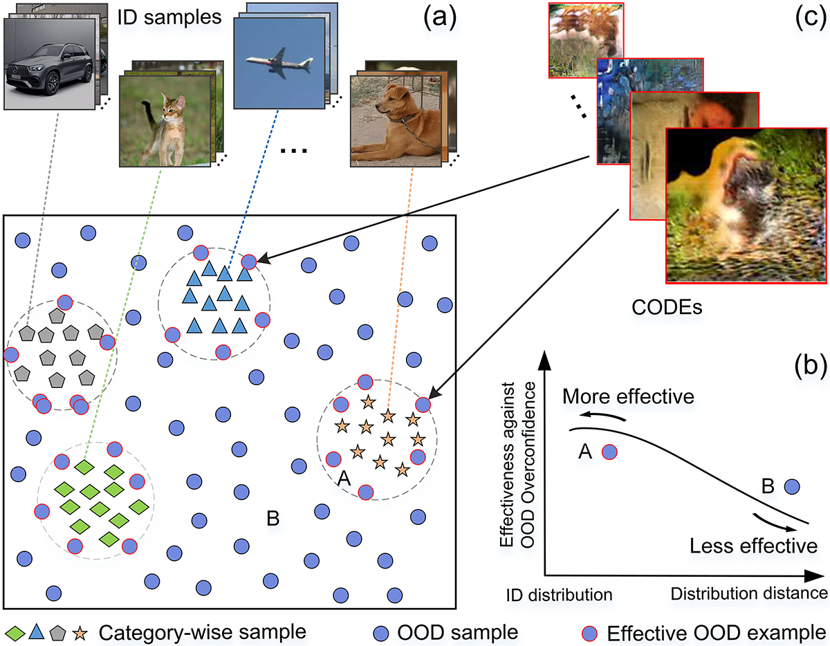
Figure 1: For a classification task, (a) OOD samples can be infinitely outnumber ID samples; (b) intuitively, OOD samples, whose distribution is closer to that of ID samples, are more likely to be effective against the OOD overconfidence issue; (c) we aim at generating CODEs, a kind of effective OOD examples.

Since with infinite amount, the key to resolve the OOD overconfidence issue is to build a subset of OOD samples and then suppress predictions on them. Lee et al. [27] use a generative adversarial network [12] to model the subset which, however, requires to be tuned on the testing-distribution. Without synthesizing data from a carefully designed distribution, Hendrycks et al. [19] adopt an auxiliary dataset to simulate the subset. However, the optimal choice of such dataset remains an open question, challenges of data imbalance and computational complexity make it less efficient and practical [30]. In contrast, Hein et al. [17] simply adopt random noises and permuted images, and report promising results. It thus brings us to the main topic of this paper (see Fig. 1): can we get a subset of OOD samples that is more effective for alleviating the OOD overconfidence issue by suppressing predictions on them? Intuitively, suppressing a subset of OOD samples whose distribution is close to that of in-distribution (ID) samples, are expected to bring more benefits, since they are harder to be differentiated by DNNs to make low-confident predictions. Under this hypothesis, we propose to generate a subset of OOD samples whose distribution is close to that of ID samples, i.e., effective OOD examples.

In this paper, we propose the novel Chamfer OOD examples (CODEs), which is a kind of effective OOD examples. Besides, we devise a simple yet effective method to generate CODEs with training data only. Specifically, we first generate seed examples that is OOD by slicing&splicing operations, and then feed them into the Chamfer generative adversarial network (Chamfer GAN) for distribution transformation. Particularly, the Chamfer distance loss is intentionally imposed on Chamfer GAN to maintain the pixel-level statistic of seed examples, such that CODEs remain to be OOD. We validate the effectiveness of our approach by suppressing predictions on CODEs during training. Extensive experiments show that the OOD overconfidence issue will be largely alleviated by our approach without hurting the original classification accuracy on ID samples, and that our approach outperforms the state-of-the-art methods. We also demonstrate CODEs could have broad applications, e.g., to improve OOD detectors and image classification.

Overall, our contribution is summarized as follows:

• We show distribution distance is the key factor for OOD examples in alleviating the OOD overconfidence issue, with many other factors excluded.

• We propose a simple yet effective method based on slicing&splicing operations and Chamfer GAN to generate CODEs without accessing to any extra data.

• We validate the superiority of CODEs in alleviating the OOD overconfidence issue of DNN classifiers inherently without hurting the classification accuracy.

• We demonstrate the effectiveness of CODEs in improving OOD detection and image classification.

2 Related Work

Suppressing Predictions on OOD Samples. To suppress predictions on OOD samples, Lee et al. [27] trained a classifier as well as a GAN that models the boundary of in-distribution samples, and enforced the classifier to have lower confidences on GAN samples. However, for each testing distribution, they tuned the classifier and GAN using samples from that out-distribution. Without accessing to the testing distribution directly, Hendrycks et al. [19] used an auxiliary dataset disjoint from test-time data to simulate it. Meinke et al. [34] explicitly integrated a generative model and provably showed that the resulting neural network produces close to uniform predictions far away from the training data. However, for suppressing the predictions, they also adopted auxiliary datasets. Since challenges of data imbalance and computational complexity brought by auxiliary datasets [30], Hein et al. [17] proposed to simply consider random noise and permuted images as OOD samples.

We also aim to generate OOD samples with training data only. Differently, we intentionally generate effective OOD examples, and thus obtain better results. Besides, our approach would not hurt classification accuracy on ID samples, which is not guaranteed by using auxiliary datasets.

OOD Detection. Hendrycks et al. [18] built the first benchmark for OOD detection and evaluated the simple threshold-based detector. Recent works improve OOD detection by using the ODIN score [31, 23], Mahalanobis distance [28], energy score [32], ensemble of multiple classifiers [42, 48], residual flow [51], generative models [38], self-supervised learning [20, 35] and gram matrices [39].

All above approaches detect whether a test sample is from in-distribution (i.e., training distribution by a classifier) or OOD, and is usually deployed with combining the original $n$-category classifier to handle recognition in the real world [4, 46]. Differently, our motivation is to enforce the original $n$-category classifier to make low-confident predictions on OOD samples inherently.

Confidence Calibration. The calibration of the confidence of predictions are traditionally considered on the true input distribution. Gal and Ghahramani [11] adopted Monte Carlo dropout to estimate the single best uncertainty by interleaving DNNs with Bayesian models. Lakshminarayanan et al [26] used ensembles of networks to obtain combined uncertainty estimates. Guo et al. [15] utilized temperature scaling to obtain calibrated probabilities.

Differently, our work focus on calibrating the confidence of predictions on OOD samples. Besides, it has been validated that models for confidence calibration on the input distribution cannot be used for out-of-distribution [29].

Data Augmentation. Data augmentation is originally designed to prevent networks from overfitting by synthesizing label-preserving images  [25, 10]. Another type is to improve adversarial robustness or classification performance by adding adversarial noise to the training images [33, 44].

Differently, we suppress the predictions on the augmented images which are OOD, while augmented ID images in their methods are trained in the same manner as original training data.

3 Effective OOD Examples

Preliminary.   This work considers the setting in multi-category classification problems. Let $\mathcal{A}$ be the set of all digital images under consideration and $\mathcal{I}\subseteq\mathcal{A}$ be the set of all in-distribution samples that could be assigned a label in $\{1,2,...,K\}$. Then, $\mathcal{A}\setminus\mathcal{I}$ is the set of all OOD samples. Specifically, we have a classifier $f:\mathcal{I}\rightarrow\{1,2,...,K\}$ that could give a prediction for any image in $\mathcal{A}$.

Indeed, the classifier $f$ could make high-confident predictions on images in $\mathcal{A}\setminus\mathcal{I}$. It is thorny when DNN classifiers face an open-set world. Since OOD samples can be infinitely many, suppressing them all is impractical. We thus aim at collecting a subset of OOD samples that are effective for alleviating the OOD overconfidence issue by suppressing predictions on them, i.e., effective OOD examples.

Definition 1

Effective OOD Examples. Given a small constant $\delta$, an effective OOD example $x$ is any image in $\mathcal{S}_{eo}$ satisfying

$$\mathcal{S}_{eo}\triangleq\{x\in\mathcal{A}\setminus\mathcal{I}\ |\ D(P_{\mathcal{I}},P_{eo})\leq\delta\},$$

where $P_{\mathcal{I}}$ is the distribution of $\mathcal{I}$, $P_{eo}$ is the distribution of $\mathcal{S}_{eo}$, and $D$ is the criterion to measure the distance between two distributions.

Since $P_{eo}$ is close to that of in-distribution samples $P_{\mathcal{I}}$, it is hard to differentiate them. Therefore, suppressing effective OOD examples is expected to bring more benefits than suppressing the others that are easier to be differentiated.

4 Method

In this section, we will introduce the approach to obtain effective OOD examples with training data only. Particularly, we start by generating seed examples that are OOD, then convert those seeds into Chamfer OOD examples (CODEs) by enforcing the distribution restriction. Finally, we will demonstrate how to alleviate the OOD overconfidence issue by training with CODEs.

4.1 Generating Seed Examples

We generate seed examples by splicing local patches from images with multiple different categories via two key operations.

Slicing Operation:

$$\{p_{0}^{x},p_{1}^{x},...,p_{k*k-1}^{x}\}= OP_{slice}(x,k)$$ (1)

where $x$ is an image in the training set and $p_{t}^{x}$ is the $t$-th piece of $x$. By this operation, each image is divided into $k\times k$ numbers of patches equally (see Fig. 2).

Figure 2: Generate seed examples by slicing and splicing ($k=3$).

Splicing Operation:

$$\overline{x}=OP_{splice}([p_{0}^{x^{0}},p_{1}^{x^{1}},...,p_{k*k-1}^{x^{k*k-1}}],k)$$ (2)

$$st.\ \ (c(x^{0})==c(x^{1})==...==c(x^{k*k-1}))=False$$

where $k\times k$ numbers of patches with uniform size that are sliced from images with different categories (denoted by $c(\cdot)$) are spliced into an image with the same size as $x$ (see Fig. 2). Particularly, those patches are required to be not from images with the same categories.

Since the resulting seed examples do not belong to any categories visually (see Fig. 2), and thus are OOD examples. Note that, we just provide two simple operations for the splicing of image patches. More complex operations (e.g., considering angles, scales and rotation) could be extended easily, but is out of the scope of this paper.

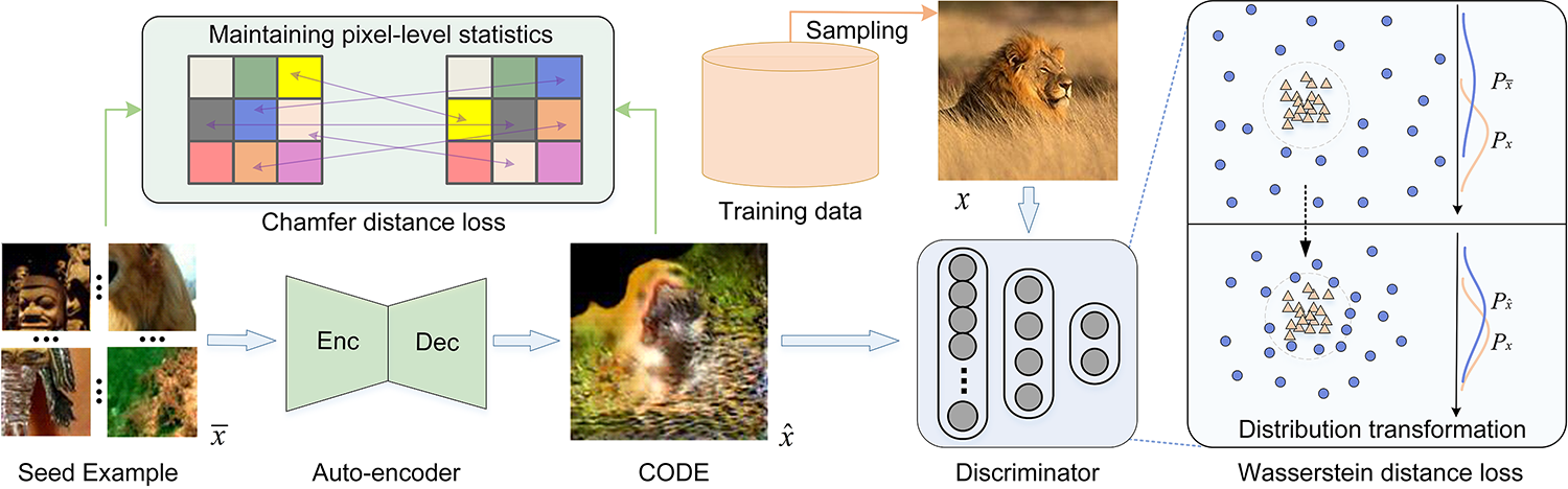
Figure 3: The framework of Chamfer GAN: given a seed example $\bar{x}$ as input, the auto-encoder backbone outputs the CODE $\hat{x}$; it is supervised by the Chamfer distance loss for maintaining pixel-level statistics and the Wasserstein distance loss for transforming the distribution $P_{\hat{x}}$ to $P_{{x}}$.

4.2 Generating CODEs

We transform the distribution of seed examples to that of the training data by feeding them into a novel Chamfer generative adversarial network (Chamfer GAN) with maintaining pixel-level statistics, to generate CODEs. In this following, we will describe the architecture design of Chamfer GAN first, and then discuss why CODEs generated by Chamfer GAN are effective OOD examples.

4.2.1 Chamfer GAN

For the design of Chamfer GAN, we adopt the popular auto-encoder [22] as our backbone, see Fig. 3. Given a seed example $\bar{x}$ as input, the encoder $Enc$ projects it into high-dimensional compact space, and the decoder $Dec$ decode the projected feature to reconstruct the CODE $\hat{x}$. Particularly, we adopt the Wasserstein distance loss in WGAN [14] to transform the data distribution, and the Chamfer distance loss  [5] to maintain pixel-level statistics.

Wasserstein distance loss.   To enforce the distribution of $\hat{x}$ (i.e., $P_{\hat{x}}$) to be close to that of the training data $x$ (i.e., $P_{x}$), we adopt the same adversarial loss as in WGAN [14] with the gradient penalty term omitted for clarity, which is defined as:

$$L_{\text{WD}}={\mathbb{E}_{x\sim P_{x}}}[Dis(x)]-{\mathbb{E}_{\hat{x}\sim P_{\hat{x}}}}[Dis(\hat{x})]$$ (3)

Chamfer distance loss.   To facilitate maintaining pixel-level statistics during the reconstruction process, we adopt the Chamfer distance for restriction, which is defined as:

$$L_{\text{CD}}={{\mathbb{E}}_{\bar{x}{\sim}P_{\bar{x}}}}\bigg{(}{\sum_{\hat{x_{i}}\in\hat{{x}}}\min_{\bar{x_{j}}\in\bar{x}}\|\hat{x_{i}}-\bar{x_{j}}\|_{2}^{2}}+\sum_{\bar{x_{j}}\in\bar{x}}\min_{\hat{x_{i}}\in\hat{{x}}}{\|\hat{x_{i}}-\bar{x_{j}}\|_{2}^{2}}\bigg{)}$$ (4)

$$\hat{x}=Dec(Enc(\bar{x}))$$ (5)

where $P_{\bar{x}}$ is the distribution that seed example $\bar{x}$ is in, $\bar{x_{j}}$ and $\hat{x_{i}}$ denote the pixel in $\bar{x}$ and $\hat{x}$ respectively. Note that, we do not require $\bar{x}$ and $\hat{x}$ to be extremely the same which is enforced by $L_{2}$ loss in traditional auto-encoder. Instead, the Chamfer distance loss enforces each pixel in $\bar{x}$ to have a corresponding pixel in $\hat{x}$ outputted by $Enc$-$Dec$, but could at a different location, namely with pixels rearranged. Therefore, the pixel-level statistics is maintained.

By combining the above two loss functions, Chamfer GAN could transform the distribution of ${\hat{x}}$ to be close to that of the training data $x$, while maintaining the pixel-level statistics of $\bar{x}$. The final loss function is thus as follows:

$$L_{\bar{x}\rightarrow\hat{x}}={\alpha}L_{\text{WD}}+L_{\text{CD}}$$ (6)

where $\alpha$ is a scalar weight set by $1.0\mathrm{e}{-5}$ by default. For the training of Chamfer GAN, we train the classifier $Dis$ and $Enc$-$Dec$ in an iterative manner as in WGAN. Note that, the Chamfer distance loss is critical for Chamfer GAN. Specifically, Chamfer distance loss restricts the distribution transforms along a special feature space whose corresponding image space is a “pixel rearranged space”.

By feeding seed examples into Chamfer GAN, CODEs are obtained that maintain pixel-level statistics of seed examples, but within a distribution much closer to that of the training data.

4.2.2 Discussion on CODEs

Since with supervision by the Wasserstein distance loss, the distribution of CODEs is transformed to be close to that of the training data. Besides, CODEs remain to be OOD, due to: 1) the pixel-level statistics of seed examples that are originally OOD are maintained by the Chamfer distance loss; and 2) the training of WGAN that transforms the distribution to be the same as that of the training data is hard originally, and it is even harder with the restriction of Chamfer distance loss. Overall, CODEs are effective OOD examples. Please refer to Sec. 5.1 for validation.

4.3 Using CODEs against OOD Overconfidence

CODEs could be utilized to alleviate the OOD overconfidence issue by suppressing predictions on them over each category, namely enforcing averaged confidences over all categories (i.e., $\frac{1}{K}$) with the following loss function:

$$L_{sup}(\hat{x})=\sum_{i=1}^{i=K}\frac{1}{K}\log{V_{i}(\hat{x})}$$ (7)

where $K$ is the category number and $V_{i}(\hat{x})$ is the normalized prediction confidence of $\hat{x}$ over category $i$.

For training, we adopt 50% images from the original training set supervised with the cross-entropy loss, while the others are CODEs supervised with Eqn. 7.

5 Experiments

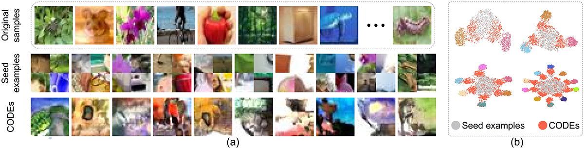
Figure 4: (a) Row-1: original images from CIFAR-100; Row-2: seed examples; Row-3: the corresponding CODEs of Row-2. (b) The t-SNE embeddings of original images (2, 3, 6 and 10 categories), seed examples and CODEs on CIFAR-10.

This section includes four parts. Firstly, we analyze the features of CODEs. Secondly, we extensively evaluate CODEs for alleviating the OOD overconfidence issue inherently with comparing with the state-of-the-art methods. Thirdly, we demonstrate the applications of CODEs, e.g., for improving OOD detection and classification. Finally, we report the ablation studies.

5.1 Features of CODEs

Implementation.   We set $k$ as 2 for generating seed examples. The auto-encoders in Chamfer GAN for 32$\times$32 and 28$\times$28 images adopt four convolution layers to project images to the resolution of 2$\times$2 with channel number of 512, while the decoder is symmetric to the encoder, except replacing the convolutions with transposed ones. For $224\times 224$ images, we adopt the architecture in [2]. We train the Chamfer GAN with a batch size of 32 for 1800 epochs on CIFAR-10 and CIFAR-100, 800 epochs on SVHN, MNIST, FMNIST and CINIC-10, and 50 epochs on ImageNet. The optimizer and learning rate are the same as in WGAN [14]. For more details, please refer to the supplementary.

Visualization.   Fig. 4(a) visualizes seed examples, the corresponding CODEs, and original images from CIFAR-100. Visually, CODEs are more natural than seed examples, but we could not induce any categories on them, indicating that they are OOD examples. Fig. 4(b) visualizes the t-SNE [41] embeddings of original images, seed examples and CODEs on CIFAR-10. Specifically, the embeddings are based on the features outputted by the last convolutional layer of ResNet-18. It demonstrates that the distributions of CODEs are much closer to that of clusters of original images compared with seed examples, validating the usefulness of Chamfer GAN for distribution transformation.

Distribution Distance and Prediction Confidence.   We report the distribution distances between seed examples, CODEs and the original images in CIFAR-10, CIFAR-100 and SVHN, measured by Fréchet Inception Distance (FID) [21] in Tab. 1. It could be seen that the distribution distances between CODEs and original images are much smaller than that of seed examples, validating the process of distribution transformation. Particularly, with a closer distribution to that of the original images, CODEs are predicted by ResNet-18 with higher confidences.

		CIFAR-10	CIFAR-100	SVHN
FID	Seeds examples	50.49	48.83	83.51
	CODEs	36.53	36.53	77.94
MMC (%)	Origin	98.40	91.28	99.42
	Seeds examples	72.53	38.90	72.37
	CODEs	74.84	40.20	78.74

Table 1: Distribution distances of seed examples and CODEs to that of original datasets measured by FID, and the prediction confidences on them measured by mean maximum confidence (MMC).

5.2 Alleviating OOD Overconfidence by CODEs

train set	metric	test set	Baseline	CEDA	ACET	CCUs	Ours	Ours++	OE	CCUd
with auxiliary dataset									✓	✓
CIFAR-10	TE	CIFAR-10	5.38	5.38	5.61	5.56	5.58	5.52	5.75	6.01
	ID MMC	CIFAR-10	97.04	97.51	96.60	97.27	97.15	96.77	88.87	80.26
	OOD MMC	SVHN	73.38	72.46	70.69	74.13	62.37	47.18	10.48	10.41
		CIFAR-100	79.47	80.54	79.28	80.83	70.14	59.52	21.62	16.98
		LSUN_CR	73.38	75.15	75.89	75.95	64.11	53.67	10.56	10.38
		Noise	69.24	10.36	10.62	77.85	10.27	10.89	13.37	10.36
		Uniform	99.49	73.23	10.00	10.00	65.30	10.00	10.35	10.00
		Adv. Noise	100.00	98.50	11.20	10.01	15.80	10.29	100.00	10.00
		Adv. Samples	100.00	100.00	63.30	-	54.40	27.79	-	-
CIFAR-100	TE	CIFAR-100	23.34	23.54	24.01	24.13	23.22	23.55	25.51	26.53
	ID MMC	CIFAR-100	80.54	81.85	80.64	81.78	82.21	80.77	59.55	47.29
	OOD MMC	SVHN	61.15	57.91	39.54	51.02	44.34	32.50	3.96	2.26
		CIFAR-10	52.13	55.23	54.30	55.58	52.82	49.10	15.56	8.49
		LSUN_CR	53.19	51.41	54.22	52.34	51.33	48.01	3.10	1.60
		Noise	61.40	57.89	19.27	57.67	19.96	14.92	10.94	7.84
		Uniform	59.62	34.05	1.00	1.00	1.77	1.00	2.03	1.00
		Adv. Noise	100.00	98.50	1.30	1.00	6.50	1.00	100.00	1.00
		Adv. Samples	99.90	99.90	86.30	-	12.90	4.30	-	-
SVHN	TE	SVHN	2.89	2.88	3.05	3.07	3.02	2.84	4.05	3.05
	ID MMC	SVHN	98.47	98.58	98.52	98.62	98.45	98.69	96.93	98.07
	OOD MMC	CIFAR-10	71.94	71.70	69.28	68.40	61.09	50.78	10.14	10.14
		CIFAR-100	71.76	71.04	68.78	68.63	54.09	53.46	10.16	10.20
		LSUN_CR	71.27	71.06	62.18	65.78	36.45	29.98	10.14	10.09
		Noise	72.00	68.87	39.89	63.43	35.58	33.53	35.57	48.81
		Uniform	67.80	40.06	10.00	10.00	10.34	10.00	10.10	10.00
		Adv. Noise	100.00	94.60	10.10	10.00	24.30	11.00	100.00	10.00
		Adv. Samples	100.00	99.50	36.90	-	38.70	11.40	-	-
MNIST	TE	MNIST	0.51	0.50	0.50	0.49	0.47	0.51	0.75	0.51
	ID MMC	MNIST	99.18	99.16	99.15	99.16	98.99	99.34	99.27	99.16
	OOD MMC	FMNIST	66.31	52.88	28.58	63.93	35.32	20.98	34.38	25.99
		EMNIST	81.95	81.81	77.92	83.01	69.54	47.78	88.00	77.74
		GrCIFAR-10	46.41	19.10	10.10	10.02	10.43	10.00	11.50	10.00
		Noise	12.70	12.09	10.36	10.59	10.51	10.00	10.22	10.34
		Uniform	97.33	10.01	10.00	10.00	10.01	10.40	10.01	10.00
		Adv. Noise	100.00	14.70	16.20	10.00	12.50	10.00	100.00	10.00
		Adv. Samples	99.90	98.20	85.40	-	63.80	45.20	-	-
FMNIST	TE	FMNIST	4.77	5.01	4.78	4.85	4.56	4.79	6.12	4.96
	ID MMC	FMNIST	98.38	98.24	98.03	98.32	98.44	98.35	98.30	98.46
	OOD MMC	MNIST	71.32	73.44	73.70	71.25	69.67	61.47	80.34	70.54
		EMNIST	65.01	67.34	66.63	68.68	62.97	59.13	36.66	31.62
		GrCIFAR-10	86.17	69.69	72.90	56.33	66.88	63.24	10.22	10.09
		Noise	67.72	57.40	16.75	56.84	14.71	13.03	10.45	10.25
		Uniform	77.70	60.08	10.00	20.00	10.00	10.06	73.16	10.00
		Adv. Noise	100.00	22.30	16.78	10.00	14.99	10.18	100.00	10.00
		Adv. Samples	100.00	99.67	90.56	-	70.14	59.43	-	-

Table 2: We train eight models on five datasets and evaluate them on the original dataset and OOD samples, including other datasets, Noise, Uniform, Adversarial (Adv.) Noise and Adversarial Samples. We report the test error (TE) $\downarrow$ of all models, show mean maximum confidence (MMC) on in- and out-of-distribution samples (e.g., ID MMC $\uparrow$ and OOD MMC $\downarrow$). All values are in percent (%).

Datasets.   Various datasets are used: CIFAR-10, CIFAR-100 [24], GrCIFAR-10 (gray scale CIFAR-10), SVHN [36], LSUN_CR (the classroom subset of LSUN [47]), MNIST, FMNIST [43], EMNIST [7], Noise (i.e., randomly permuting pixels of images from the training set as in [34]), Uniform (i.e., uniform noise over the $[0,1]^{d}$ box as in [34]), Adversarial Noise and Adversarial Sample following the experimental setting as [34]. Adversarial Noise is generated by actively searching for images which yield higher prediction confidences in a neighbourhood of noise images, while Adversarial Sample is generated in a neighbourhood of in-distribution images but are off the data manifold following [17]. For OE and CCUd, we adopt 80 Million Tiny Images [40] with all examples that appear in CIFAR-10 and CIFAR-100 removed as the auxiliary dataset as in [34].

Methods.   Eight methods are evaluated and compared: Baseline, CEDA [17], ACET [17], OE [19], two variants of CCU [34] (CCUs that adopts noise and CCUd that adopts an auxiliary dataset as in [19]), Ours and Ours++. Particularly, Ours++ is an enhanced version of Ours, with selecting the worst cases, i.e., have the largest prediction confidences, in a neighborhood of CODEs similar as in ACET [17].

Setup. We train LeNet on MNIST and FMNIST while ResNet-18 for CIFAR-10, CIFAR-100 and SVHN, and then evaluate them on the corresponding test set to report the test error (TE), and on both in- and out-of-distribution datasets to report mean maximal confidence (MMC) following [34].

Comparisons with the State-of-the-art Methods.   The results in Tab. 2 show that Ours and Ours++ perform the best in most cases without considering OE and CCUd on CIFAR-10, CIFAR-100 and SVHN. Since training with suppressing the predictions on the large 80 Million Tiny Images [40], that has similar image style as the OOD datasets (e.g., CIFAR-10, CIFAR-100 and SVHN), OE and CCUd obtain the lowest MMCs. However, it could be seen that the auxiliary dataset brings a detrimental impact on the predictions on in-distribution samples, e.g., 33% lower prediction confidences on CIFAR-100 for CCUd, and thus leads to worse classification performance, e.g., 3.2% larger test error. Besides, for datasets that have large differences with the auxiliary dataset, OE and CCUd are comparable with and even worse than Ours and Ours++, e.g., on FMNIST and MNIST.

Particularly, ACET performs better than CEDA, validating the usefulness of the strategy that searches harder examples in a neighbourhood of the original ones. We would like to point out that our method is comparable with ACET even without picking harder examples, indicating that CODEs are more effective than random noises. By applying the same strategy to Ours, we could see significant drops in MMC values. For Adversarial Noise and Adversarial Sample, we could see that CEDA and OE fail in most cases, ACET could handle part of samples, while Ours++, CCUs and CCUd perform the best. Overall, CODEs are effective in alleviating the OOD overconfidence issue.

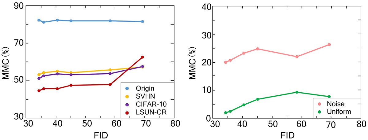
Figure 5: The distribution distances between CODEs and the training data measured by FID versus the MMCs on the original dataset (Origin) and various OOD datasets, Noise and Uniform made by ResNet-18 trained on CIFAR-100.

Distribution Distance vs. MMC.   We investigate how distribution distance between CODEs and the in-distribution data would affect the benefits brought by suppressing CODEs on alleviating the OOD overconfidence issue. Since we apply a relatively high weight $1.0$ to the Chamfer distance loss, while a low weight $1.0\mathrm{e}{-5}$ to Wasserstein distance loss, the distribution transforming could be carried on gradually during the training process. To facilitate fair comparisons, we choose the models of Chamfer GAN saved at different epochs during the training stage on CIFAR-100, including models of 200$th$, 400$th$, 800$th$, 1200$th$, 1600$th$ and 1800$th$, and then train ResNet-18 models with suppressing predictions on the CODEs outputted by the above six Chamfer GANs respectively. Fig. 5 shows that MMCs are mostly positively relevant to the FID scores, and the correlation is stronger on OOD datasets than on Noise and Uniform, validating that smaller distribution distance to the in-distribution samples is critical for effective OOD examples. We also report the MMCs on in-distribution samples of the six different ResNet-18 models in Fig. 5, and could see the MMCs mostly remain unchanged.

Indeed, OE have also mentioned the influence of distribution distance [19]. However, since the difference between different auxiliary datasets could have many different factors, e.g., RGB values, local textures, it is thus not suitable to conclude which factor affects the result. Differently, we transform the distribution of seed examples with Chamfer distance loss to maintain the low-level pixel statistics, such that could rule out the influence of many other factors.

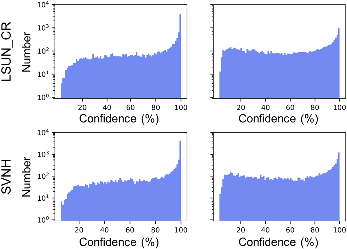
Figure 6: Histograms (logarithmic scale) of maximum confidence values of ResNet-18 trained for CIFAR-100 on various datasets.

Visualization of Maximum Confidence.   We visualize the maximum confidences predicted on the images in LSUN_CR and SVHN by ResNet-18 trained on CIFAR-100 using logarithmic histograms in Fig. 6. It could be seen that, by adopting our method, the confidence distributions made by Baseline are pulled to the left, with the number of samples with high confidence largely reduced.

In-distribution Confidence Calibration.   We report expected calibration errors (ECEs) [15] of ResNet-18 trained on CIFAR-10/100 and test on the corresponding test set in Tab. 3. It could be seen that ECEs are reduced after applying our method, while temperature tuning is more effective in calibrating prediction confidence on in-distribution data.

	CIFAR-10		CIFAR-100
	Before TT	After TT	Before TT	After TT
w/o Ours	0.033	0.031	0.081	0.073
w/ Ours	0.008	0.006	0.059	0.042

Table 3: Expected calibration errors (ECEs) $\downarrow$ on CIFAR-10 and CIFAR-100 w/ and w/o Ours and temperature tuning (TT).

5.3 Applications of CODEs

5.3.1 Improving OOD Detection

Evaluation Strategy and Metrics.   We follow the evaluation strategy as in [18] and use the three common metrics: the false positive rate of OOD examples when true positive rate of in-distribution examples is at 95% (FPR95), the area under the receiver operating characteristic curve (AUROC), and the area under the precision-recall curve (AUPR).

		FPR95 $\downarrow$	AUROC $\uparrow$	AUPR $\uparrow$
CIFAR-10	OE	8.53	98.30	99.63
	OE+CODEs	8.01	99.07	99.79
	ES	3.32	98.92	99.75
	ES+CODEs	3.24	99.01	99.78
CIFAR-100	OE	58.10	85.19	96.40
	OE+CODEs	56.54	87.96	97.38
	ES	47.55	88.46	97.12
	ES+CODEs	45.89	89.03	97.95

Table 4: The improvement brought by CODEs on OE [19] and Energy Score (ES) [32]. All values are in percent (%).

Methodology.   We replace the original DNN classifier with the one trained with suppressing predictions on CODEs.

Improving OOD detectors.   We first evaluate the improvement on OE [19] and Energy Score [32] that use 80 Million Tiny Images [40] as the auxiliary dataset. Specifically, we train WRN-40-2 [49] on CIFAR-10 and CIFAR-100 [24], and then test it on six datasets: Textures [6], SVHN, Places365 [50], LSUN-Crop [47], LSUN-Resize [47], and iSUN [45] following [32]. The averaged results in Tab. 4 show that the performance on all three metrics are improved. We also evaluate the improvement on ODIN [31] and Mahalanobis distance (Maha) [28] that do not require auxiliary datasets. The results in Tab. 5 show that both ODIN and Maha are improved. Overall, CODEs could be adopted for improving OOD detectors.

		ODIN	ODIN+CODEs	Maha	Maha+CODEs
	CIFAR-10	95.91	96.90	97.10	97.34
	CIFAR-100	94.82	97.12	96.70	97.08
	LSUN_CR	96.52	96.96	97.22	97.97
	Noise	82.74	83.01	98.00	97.99
SVHN	Uniform	97.90	97.94	97.81	98.01
	SVHN	81.35	84.91	77.52	79.63
	CIFAR-10	79.50	83.48	59.94	64.74
	LSUN_CR	81.41	82.10	79.73	82.99
	Noise	76.84	76.92	90.61	90.98
CIFAR-100	Uniform	93.56	94.87	94.37	95.90

Table 5: The improvement brought by CODEs on ODIN [31] and Mahalanobis distance (Maha) [28] in the AUROC metric (%) $\uparrow$.

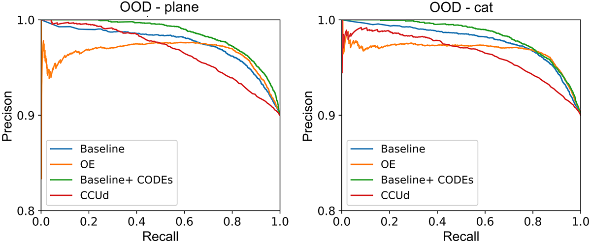
Figure 7: PR curves of four methods for the semantic OOD detection task [1] on CIFAR-10 with holding out one class as OOD.

		Baseline	Baseline+CODEs
CINIC-10	ResNet-32	73.82	74.77
	ResNet-56	74.09	75.38
ImageNet	ResNet-18	69.76	71.06
	ResNet-50	76.15	77.12

Table 6: Top-1 Acc (%) $\uparrow$ on CINIC-10 and ImageNet.

Detecting Semantic OOD Examples.   We evaluate the situation where in-distribution samples are not only significantly outnumber OOD ones, but also have significant semantic shifts following [1]. Specifically, we train two classifiers for CIFAR-10 with holding out one class every time (e.g., plane, cat), and then score the ability to detect the held out class as OOD samples. The precision-recall curves are presented in Fig. 7. It could be seen that OE [19] and CCUd [34] that adopt auxiliary datasets hurt the performance of semantic OOD detection since predictions on in-distribution samples are suppressed as reported in Tab. 2, while utilizing CODEs is beneficial to it.

5.3.2 Improving Classification

We demonstrate CODEs could improve classification by evaluating ResNets on CINIC-10 [8] and ImageNet [9]. Particularly, a separate batch norm for CODEs is adopted following [44], which is critical for consistent improvement. The results in Tab. 6 show that CODEs bring 1-2 percent improvement on the top-1 accuracy. The reason is probably that CODEs are sampled in between the decision boundaries of multiple categories since are spliced with patches from different-category images, and thus could help to prevent confusion between multiple different categories.

	CIFAR-100	CIFAR-10	SVHN
Baseline	78.99	57.50	70.95
w/o Chamfer GAN	50.23	58.08	59.67
w/ Chamfer GAN	43.64	54.44	51.62

Table 7: Ablation study on Chamfer GAN with averaged MMC (%) $\downarrow$ tested on OOD datasets listed in Tab. 2.

$k$	2	4	6	8
MMC	43.64	47.89	46.32	48.39

Table 8: Averaged MMC (%) $\downarrow$ of ResNet-18 (trained on CIFAR-100) tested on OOD datasets listed in Tab. 2.

5.4 Ablation Studies

Setup.   We train different ResNet-18 models with suppressing predictions on CODEs generated with/without Chamfer GAN, and with different $k$s in the slicing&splicing operations, and then test them on OOD datasets listed in Tab. 2 to report averaged MMC results in Tab. 7 and Tab. 8.

Chamfer GAN.   It could be seen that ResNet-18 models trained with ablating Chamfer GAN still improve the performance, since the distribution of seed examples are originally close to the ID distribution with the novel slicing&splicing operation as reported in Tab. 2. However, the performance is much worse than that with Chamfer GAN, validating the importance of distribution transformation.

Piece $k$.   It could be seen that $k=2$ brings the best performance in Tab. 8, since larger $k$ may bring too more flexibility for Chamfer GAN to maintain the pixel-level statistics.

6 Conclusion

This paper has proposed CODEs, a kind of effective OOD examples that could be utilized to alleviate the OOD overconfidence issue inherently by suppressing predictions on them. The key idea of generating CODEs is to restrict the distribution of spliced OOD examples generated from training data, to be close to that of in-distribution samples by Chamfer GAN. Extensive experiments validate the effectiveness of CODEs and their usefulness in improving OOD detection and classification. We hope CODEs inspire more research on alleviating the OOD overconfidence issue.

Acknowledgements: This work was supported in part by the Guangdong Basic and Applied Basic Research Foundation (2020A1515110997), the NSFC (U20B2046, 61902082, 62072126), the Science and Technology Program of Guangzhou (202002030263, 202102010419), the Guangdong Higher Education Innovation Group (2020KCXTD007) and the Talent Cultivation Project of Guangzhou University (XJ2021001901).

References

- [1] Faruk Ahmed and Aaron Courville. Detecting semantic anomalies. In AAAI, volume 34, pages 3154–3162, 2020.
- [2] Vijay Badrinarayanan, Alex Kendall, and Roberto Cipolla. Segnet: A deep convolutional encoder-decoder architecture for image segmentation. IEEE TPAMI, 39(12):2481–2495, 2017.
- [3] Abhijit Bendale and Terrance Boult. Towards open world recognition. In CVPR, pages 1893–1902, 2015.
- [4] Abhijit Bendale and Terrance E Boult. Towards open set deep networks. In CVPR, pages 1563–1572, 2016.
- [5] Gunilla Borgefors. Hierarchical chamfer matching: A parametric edge matching algorithm. IEEE TPAMI, 10(6):849–865, 1988.
- [6] Mircea Cimpoi, Subhransu Maji, Iasonas Kokkinos, Sammy Mohamed, and Andrea Vedaldi. Describing textures in the wild. In CVPR, pages 3606–3613, 2014.
- [7] Gregory Cohen, Saeed Afshar, Jonathan Tapson, and Andre Van Schaik. Emnist: Extending mnist to handwritten letters. In IJCNN, pages 2921–2926. IEEE, 2017.
- [8] Luke N Darlow, Elliot J Crowley, Antreas Antoniou, and Amos J Storkey. Cinic-10 is not imagenet or cifar-10. arXiv preprint arXiv:1810.03505, 2018.
- [9] Jia Deng, Wei Dong, Richard Socher, Li-Jia Li, Kai Li, and Li Fei-Fei. Imagenet: A large-scale hierarchical image database. In CVPR, pages 248–255, 2009.
- [10] Terrance DeVries and Graham W Taylor. Improved regularization of convolutional neural networks with cutout. arXiv preprint arXiv:1708.04552, 2017.
- [11] Yarin Gal and Zoubin Ghahramani. Dropout as a bayesian approximation: Representing model uncertainty in deep learning. In ICML, pages 1050–1059. PMLR, 2016.
- [12] Ian J Goodfellow, Jean Pouget-Abadie, Mehdi Mirza, Bing Xu, David Warde-Farley, Sherjil Ozair, Aaron C Courville, and Yoshua Bengio. Generative adversarial nets. In NeurIPS, 2014.
- [13] Ian J. Goodfellow, Jonathon Shlens, and Christian Szegedy. Explaining and harnessing adversarial examples. In ICLR, 2015.
- [14] Ishaan Gulrajani, Faruk Ahmed, Martin Arjovsky, Vincent Dumoulin, and Aaron C Courville. Improved training of wasserstein gans. In NeurIPS, pages 5767–5777, 2017.
- [15] Chuan Guo, Geoff Pleiss, Yu Sun, and Kilian Q. Weinberger. On calibration of modern neural networks. In ICML, pages 1321–1330, 2017.
- [16] Kaiming He, Xiangyu Zhang, Shaoqing Ren, and Jian Sun. Delving deep into rectifiers: Surpassing human-level performance on imagenet classification. In ICCV, pages 1026–1034, 2015.
- [17] Matthias Hein, Maksym Andriushchenko, and Julian Bitterwolf. Why relu networks yield high-confidence predictions far away from the training data and how to mitigate the problem. In CVPR, pages 41–50, 2019.
- [18] Dan Hendrycks and Kevin Gimpel. A baseline for detecting misclassified and out-of-distribution examples in neural networks. In ICLR, 2017.
- [19] Dan Hendrycks, Mantas Mazeika, and Thomas Dietterich. Deep anomaly detection with outlier exposure. In ICLR, 2018.
- [20] Dan Hendrycks, Mantas Mazeika, Saurav Kadavath, and Dawn Song. Using self-supervised learning can improve model robustness and uncertainty. In NeurIPS, 2019.
- [21] Martin Heusel, Hubert Ramsauer, Thomas Unterthiner, Bernhard Nessler, and Sepp Hochreiter. Gans trained by a two time-scale update rule converge to a local nash equilibrium. In NeurIPS, pages 6626–6637, 2017.
- [22] Geoffrey E Hinton and Ruslan R Salakhutdinov. Reducing the dimensionality of data with neural networks. science, 313(5786):504–507, 2006.
- [23] Yen-Chang Hsu, Yilin Shen, Hongxia Jin, and Zsolt Kira. Generalized odin: Detecting out-of-distribution image without learning from out-of-distribution data. In CVPR, pages 10951–10960, 2020.
- [24] Alex Krizhevsky et al. Learning multiple layers of features from tiny images. 2009.
- [25] Alex Krizhevsky, Ilya Sutskever, and Geoffrey E Hinton. Imagenet classification with deep convolutional neural networks. In NeurIPS, volume 25, pages 1097–1105, 2012.
- [26] Balaji Lakshminarayanan, Alexander Pritzel, and Charles Blundell. Simple and scalable predictive uncertainty estimation using deep ensembles. In NeurIPS, 2017.
- [27] Kimin Lee, Honglak Lee, Kibok Lee, and Jinwoo Shin. Training confidence-calibrated classifiers for detecting out-of-distribution samples. In ICLR, 2018.
- [28] Kimin Lee, Kibok Lee, Honglak Lee, and Jinwoo Shin. A simple unified framework for detecting out-of-distribution samples and adversarial attacks. In NeurIPS, 2018.
- [29] Christian Leibig, Vaneeda Allken, Murat Seçkin Ayhan, Philipp Berens, and Siegfried Wahl. Leveraging uncertainty information from deep neural networks for disease detection. Scientific reports, 7(1):1–14, 2017.
- [30] Yi Li and Nuno Vasconcelos. Background data resampling for outlier-aware classification. In CVPR, pages 13218–13227, 2020.
- [31] Shiyu Liang, Yixuan Li, and R Srikant. Enhancing the reliability of out-of-distribution image detection in neural networks. In ICLR, 2018.
- [32] Weitang Liu, Xiaoyun Wang, John Owens, and Yixuan Li. Energy-based out-of-distribution detection. In NeurIPS, 2020.
- [33] Aleksander Madry, Aleksandar Makelov, Ludwig Schmidt, Dimitris Tsipras, and Adrian Vladu. Towards deep learning models resistant to adversarial attacks. In ICLR, 2018.
- [34] Alexander Meinke and Matthias Hein. Towards neural networks that provably know when they don’t know. In ICLR, 2020.
- [35] Sina Mohseni, Mandar Pitale, JBS Yadawa, and Zhangyang Wang. Self-supervised learning for generalizable out-of-distribution detection. In AAAI, volume 34, pages 5216–5223, 2020.
- [36] Yuval Netzer, Tao Wang, Adam Coates, Alessandro Bissacco, Bo Wu, and Andrew Y Ng. Reading digits in natural images with unsupervised feature learning. 2011.
- [37] Anh Nguyen, Jason Yosinski, and Jeff Clune. Deep neural networks are easily fooled: High confidence predictions for unrecognizable images. In CVPR, pages 427–436, 2015.
- [38] Jie Ren, Peter J Liu, Emily Fertig, Jasper Snoek, Ryan Poplin, Mark A DePristo, Joshua V Dillon, and Balaji Lakshminarayanan. Likelihood ratios for out-of-distribution detection. arXiv preprint arXiv:1906.02845, 2019.
- [39] Chandramouli Shama Sastry and Sageev Oore. Detecting out-of-distribution examples with gram matrices. In ICLR, pages 8491–8501, 2020.
- [40] Antonio Torralba, Rob Fergus, and William T Freeman. 80 million tiny images: A large data set for nonparametric object and scene recognition. IEEE TPAMI, 30(11):1958–1970, 2008.
- [41] Laurens Van der Maaten and Geoffrey Hinton. Visualizing data using t-sne. Journal of Machine Learning Research, 9(2605):2579–2605, 2008.
- [42] Apoorv Vyas, Nataraj Jammalamadaka, Xia Zhu, Dipankar Das, Bharat Kaul, and Theodore L Willke. Out-of-distribution detection using an ensemble of self supervised leave-out classifiers. In ECCV, pages 550–564, 2018.
- [43] Han Xiao, Kashif Rasul, and Roland Vollgraf. Fashion-mnist: a novel image dataset for benchmarking machine learning algorithms. arXiv preprint arXiv:1708.07747, 2017.
- [44] Cihang Xie, Mingxing Tan, Boqing Gong, Jiang Wang, Alan L Yuille, and Quoc V Le. Adversarial examples improve image recognition. In CVPR, pages 819–828, 2020.
- [45] Pingmei Xu, Krista A Ehinger, Yinda Zhang, Adam Finkelstein, Sanjeev R Kulkarni, and Jianxiong Xiao. Turkergaze: Crowdsourcing saliency with webcam based eye tracking. arXiv preprint arXiv:1504.06755, 2015.
- [46] Ryota Yoshihashi, Wen Shao, Rei Kawakami, Shaodi You, Makoto Iida, and Takeshi Naemura. Classification-reconstruction learning for open-set recognition. In CVPR, pages 4016–4025, 2019.
- [47] Fisher Yu, Ari Seff, Yinda Zhang, Shuran Song, Thomas Funkhouser, and Jianxiong Xiao. Lsun: Construction of a large-scale image dataset using deep learning with humans in the loop. arXiv preprint arXiv:1506.03365, 2015.
- [48] Qing Yu and Kiyoharu Aizawa. Unsupervised out-of-distribution detection by maximum classifier discrepancy. In ICCV, pages 9518–9526, 2019.
- [49] Sergey Zagoruyko and Nikos Komodakis. Wide residual networks. arXiv preprint arXiv:1605.07146, 2016.
- [50] Bolei Zhou, Agata Lapedriza, Aditya Khosla, Aude Oliva, and Antonio Torralba. Places: A 10 million image database for scene recognition. IEEE TPAMI, 40(6):1452–1464, 2017.
- [51] Ev Zisselman and Aviv Tamar. Deep residual flow for out of distribution detection. In CVPR, pages 13994–14003, 2020.