A Distributed SGD Algorithm with Global Sketching for Deep Learning Training Acceleration

Abstract

Distributed training is an effective way to accelerate the training process of large-scale deep learning models. However, the parameter exchange and synchronization of distributed stochastic gradient descent introduce a large amount of communication overhead. Gradient compression is an effective method to reduce communication overhead. In synchronization SGD compression methods, many Top-$k$ sparsification based gradient compression methods have been proposed to reduce the communication. However, the centralized method based on the parameter servers has the single point of failure problem and limited scalability, while the decentralized method with global parameter exchanging may reduce the convergence rate of training. In contrast with Top-$k$ based methods, we proposed a gradient compression method with globe gradient vector sketching, which uses the $Count-Sketch$ structure to store the gradients to reduce the loss of the accuracy in the training process, named global-sketching SGD (gs-SGD). The gs-SGD has better convergence efficiency on deep learning models and a communication complexity of O($\log d*\log P$), where $d$ is the number of model parameters and $P$ is the number of workers. We conducted experiments on GPU clusters to verify that our method has better convergence efficiency than global Top-$k$ and Sketching-based methods. In addition, gs-SGD achieves 1.3-3.1× higher throughput compared with gTop-$k$, and 1.1-1.2× higher throughput compared with original Sketched-SGD.

I Introduction

In recent years, deep learning has been widely used in various fields, especially in Computer Vision, Natural Language Processing, and Speech Recognition[1][2][3]. Most deep learning networks have achieved state-of-art performance across various domains[4][5][6]. Stochastic gradient descent (SGD) and its various variants[7] are the main methods for training deep learning networks. However, the training process of deep learning models requires large-scale datasets, like ImageNet[8]. As the networks become deeper, the parameters of the model grow quickly results in a longer training time, even taking days to weeks[9].

To improve the training efficiency of deep learning models, high-performance acceleration hardware, like NVIDIA A100[10], Google TPU[11] and Huawei Ascend910[12], are applied to reduce training time. In addition, parallel training through multiple acceleration nodes is still one of the most effective ways to reduce training time[13] significantly. Whether it is synchronous training or asynchronous training, a large number of gradient parameters need to be transmitted between servers. Compared with the computing time, the data transmission time has a delay of orders of magnitude, especially for training models that require a large number of parameter interactions, such as RNN[14]. The network communication overhead of parameter information is the fatal bottleneck to the performance of distributed training[15].

In distributed deep learning, data parallelism, model parallelism, and hybrid parallelism[16] are three commonly used methods. Data parallelism randomly divides the entire datasets into several parts, then dispatches them to different nodes. Each node maintains a complete model replica with local parameters. Model parallelism split the model into several parts delivered on different nodes. Hybrid parallelism is a combination of data and model parallelism. In general, data parallelism is suitable for large training sets, and model parallelism is ideal for large-scale models. The distributed training discussed in this paper is mainly limited to data parallelism.

Recently, many gradient compression methods, including sparsification and quantization [7][17][18][19][20] have been proposed to reduce the communication overhead between workers in training large-scale DNNs by significantly reducing the size of the exchanged gradients. The most representative one is the Top-$k$ algorithm, which significantly reduces the communication overhead in the distributed training[21]. In addition, the Sketching sparsification method [22] based on the streaming algorithm is relatively novel, which can recover favorable convergence guarantees of vanilla SGD. But these two methods use the centralized method based on the parameter server (PS), which has the single point of failure problem and limited scalability. However, other methods with the decentralized method, such as gTop-$k$ [23], still have room for improvement in convergence efficiency when training deep learning models. In this paper, we use the Count Sketch to compress the gradient on the local workers, which is called a sketch. Then we first propose the tree structure All-Reduce algorithm to aggregate the sketches from workers. Compared with gTop-$k$ and Sketched-SGD, we reduce the communication complexity from O($k\log P$) and O($\log d*P$) to O($\log d*\log P$) respectively without affecting the convergence rate of the model. The gs-SGD achieves 1.3-3.1× acceleration effect compared with gTop-$k$, and 1.1-1.2× speedup than original Sketched-SGD. Our contributions are summarized as follows:

• We propose a global sketch sparsification algorithm on distributed synchronous SGD, called global-sketching SGD, to accelerate distributed training of deep neural networks.

• We implement the proposed gs-SGD atop popular framework PyTorch and Horovod, and evaluate the training efficiency on a 4-GPU cluster interconnected with 1Gbps Ethernet. Experiments result shows that our algorithm has significantly improved the convergence efficiency of training various CNNs, and reduces the communication time ratio among workers.

• gs-SGD achieves effectively improved training efficiency on the real-world applications with various CNNs under low-bandwidth networks (e.g., 1 Gig-Ethernet).

The rest of the paper is organized as follows. We introduce some related work in Section II, and then present our gs-SGD algorithm in Section III. Experimental results and discussions are presented in Section IV. Finally, we conclude the paper in Section V.

II Related Work

In general, data-parallel distributed SGD methods are divided into two categories: synchronous mode and asynchronous mode. This paper focuses on the gradient compression method in synchronous mode. In terms of gradient compression, sparsification and quantization are the two main methods[24][25][26]. Both centralized and distributed methods have been applied in different scenario[27][28][29].

The quantization method achieves a reduction in space occupancy by representing the gradient with a low-precision value. In 1-bit SGD [30], gradient quantization technology is used to reduce the communication overhead of distributed neural network training for the first time. In addition, the method also proposed an error feedback mechanism, which can alleviate the negative impact of gradient quantization and reduce the loss of model accuracy. signSGD[31] combined quantization with gradient direction. The paper demonstrated that it is the direction rather than the value that is significant for gradients. Therefore, even if only the sign of the gradient is kept to update the model, the training process can also converge. In some cases, this can reduce the noise of the gradient and make the convergence time shorter. A recent paper, based on previous work, realizes an adaptive quantization method[32]. In General, the value of the gradient is represented by a 32-bit variable. Therefore, there is an upper limit on the ratio of communication reduction for the quantification method, which is up to 32 times.

In contrast, the sparse method may achieve a gradient compression of hundreds of times[21]. The sparse methods reduce the space occupation by filtering some of the gradients, then discarding the remaining gradients. Filtering rules can be based on thresholds. For different models, how to determine the threshold to filter the gradient is a difficult problem. Therefore, some adaptive methods have also been proposed[33]. Besides thresholds, Top-$k$ compression is a widely used sparse method[34][21]. DGD (Distributed Gradient Descent)[34] is an exploratory work. The training speed can be significantly improved by replacing dense updates in distributed SGD with sparse updates. It got 49% speedup on MNIST. DGC (Deep Gradient Compression)[21] applies momentum correction and local gradient clipping methods on top of gradient sparseness and achieves over 600 times compression. These sparse methods are mostly centralized, so there is a single point of communication bottleneck problem, especially in the harsh network communication environment. Although some methods have tried distributed gradient synchronization methods[23], they still have shortcomings in terms of convergence.

Beyond quantization and sparse methods, some vector mapping methods and data structures, like Count-Sketch[35], are applied to gradient compression[22]. The sketching data structure is mostly linear, both momentum and error accumulation can be carried out within the data. In the centralized topology, the error and momentum can be transmitted to the central node to eliminate errors and accelerate convergence[36]. This feature can also be applied to distributed gradient synchronization topology to reduce the convergence attenuation caused by gradient sparse. However, related research is rare.

Prior work has proposed applying sketching to compress the gradients on the workers in the distributed training. However, the communication complexity of these methods is high, which leads to large communication overhead. The AllReduce method used in the recently proposed gTop-$k$ effectively reduces the communication complexity of sparsification methods, but its convergence efficiency is still insufficient when training the model. The gs-SGD proposed in this paper has the same low communication complexity as gTop-$K$ and has higher convergence efficiency. The gs-SGD scheme effectively speeds up the training efficiency of various real-world applications of CNNs on GPU clusters under low-bandwidth networks (e.g., 1 Gig-Ethernet).

III Methods

III-A SGD with Global Sketching

In general, synchronous distributed SGD algorithms are divided into centralized algorithms based on PSs and decentralized algorithms without PSs. In a decentralized scenario, the exchange and merging process of parameters is a typical all-reduce collective communications operation[37]. Usually, we use the recursive halving and doubling method [38] to all-reduce parameters among clusters. Recursive halving and doubling process is essentially constructing a binary tree to reduce all global parameters, then backtrack the results of the recursion to all leaf nodes along the binary tree.

Various Top-$k$ compression techniques are widely used in gradient compression methods. However, when the compression ratio reaches a higher value, the Top-$k$ method significantly attenuates convergence. In addition, the Top-$k$ method must exchange both the gradient value $j$ and their coordinates $i$ when synchronizing to ensure the correct execution of the reduction, which doubled the amount of communication.

In contrast with Top-$k$ compression, there is a data structure named $Count-Sketch$. $Count-Sketch$ can compress a gradient vector $g$ into $S(g)$ with a size of $O(\frac{1}{\epsilon}\log d)$, where $\epsilon$ is a parameter to select top-$k$ largest gradient values, and $d$ is the size of $g$. $Count-Sketch$ finds all ($\alpha$ ,${\ell}_{2}$)-heavy coordinates and approximates their values with error $\pm\varepsilon\|g\|_{2}$. It does so with a memory footprint of $O(\frac{1}{\varepsilon^{2}\alpha^{2}}\log d)$. In addition, $Count-Sketch$ gained popularity in distributed systems primarily due to the merge ability property: given a sketch $S(a)$ computed on the input vector $a$ and a sketch $S(b)$ computed on input $b$, there exists a function $S(a+b)$. Note that sketching the entire vector can be rewritten as a linear operation $S(a)=Ca$, and therefore $S(a+b)=S(a)+S(b)$. We take advantage of this crucial property in gs-SGD to aggregate sketches among workers.

In gs-SGD, each worker transmits a sketch instead of its gradient. Each worker needs to compress its gradient into a $Count-Sketch$ structure locally. As shown in Lines 8 to 23 of Algorithm 1, in each iteration, two workers whose ranks are separated from each other by the value of the current iteration are taken in turn, and the latter transmits the local sketch to the former. After iterations are complete, we obtain the summed sketch on the first worker. And then, we recover the top-$k$ largest gradient elements by magnitude from the summed sketch and use the exact value of the top-$k$ to update the weight. This algorithm for recovering top-$k$ elements from a summed sketch is summarised in Algorithm 2[22].

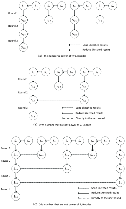
Figure 1: All-Reduce Process in gs-SGD when the number of workers is the power of 2 and non-power of 2

When $P$ is not a power of 2, Algorithm 1 needs some minor improvements. In Fig. 1(a), $P$ is power of two and Algorithm 1 works. In Fig. 1(b) and Fig. 1(c), $P$ is not power of two. From the initial round, when the number of nodes participating in the reduce is odd, the node with the largest id goes directly to the next round without participating in this round of recursive halving. Through mathematical induction, we can get that no matter the initial value is odd or even, it will eventually recurse to a unique root node. Therefore, no matter whether $P$ is a power of 2, we need at most $2\lceil\log P\rceil$ rounds to get all-reduce sketch results and pass them back to all workers.

Algorithm 1 Global Sketching SGD

1:The dataset: $D$

2:The initialized weights: $w$

3:The number of non-zero elements: $k$

4:The number of workers $P$

5:The rank of worker $g$

6:The learning rate $\eta$

7:The number of iterations to train: $T$

8:initialize the stochastic gradient $G^{g}_{0}=0$

9:for $t=1\rightarrow T$ do

10:     Sampling a mini-batch of data $D^{g}_{t}$ from $D;$

11:     Compute stochastic gradient $\widetilde{G}^{g};$

12:     Compute sketches ${S}_{t}^{g}$ of $\widetilde{G}^{g}$

13:     $sends={S}_{t}^{g};$

14:     Initialize $recvs$ with the same as $sends;$

15:     $nRounds=\log P;$

16:     for $i=1\rightarrow nRounds$ do

17:         $pRanks=[1\rightarrow P,step=i];$

18:         if $i=1\rightarrow nRounds$ then

19:              $localRank=pRanks.index(g);$

20:              if $localRank\%2==0$ then

21:                  $source=pRanks[localRank+1];$

22:                  Recv($recvs$, source=$source$);

23:                  $sends=recvs+sends;$

24:              else

25:                  $target=pRanks[localRank-1];$

26:                  Send($sends$, dest=$target$);

27:              end if

28:         end if

29:         $S_{t}=sends$

30:     end for

31:     $\widetilde{G}_{t}=HEAVYMIX(S_{t},k)$

32:     Update $w_{t+1}=w_{t}-\eta\widetilde{G}_{t}$

33:end for

Algorithm 2 HEAVYMIX[22]

1:Sketch of gradient: $S$

2:The number of non-zero elements: $k$

3:The rank of worker: $g$

4:$\widetilde{g}:\forall{i}\in Top_{k}:\widetilde{g}_{i}=g_{i}$ and $\forall{i}\notin{Top_{k}}:\widetilde{g}_{i}=0$

5:$\forall{i}$ query $\hat{g}^{2}_{i}\pm\frac{1}{2k}||g||^{2}_{2}$ from sketch $S$

6:$H\leftarrow{i|\hat{g}_{i}\geq\hat{l}^{2}_{2}/k}$ and $NH\leftarrow{i|\hat{g}_{i}<\hat{l}^{2}_{2}/k}$

7:$Top_{k}=H\cup rand_{l}(NH),$ where $l=k-|H|$

8:second round of communication to get exact values of Top_k

III-B Communication Complexity analysis

The communication nodes discussed in this article are all available GPU servers, which use the TCP/IP protocols to communicate to send and receive data simultaneously. For the communication complexity analysis, the cost of gradient exchanging between two nodes will be modeled by $\alpha+n\beta$ without considering network conflicts where $\alpha$ is message startup time, and $\beta$ is transmission time per data. Since all communication nodes are in the same data center, the communication time gap due to distance is negligible. In general, $\alpha$ is four to five orders of magnitude greater than $\beta$[37].

In gs-SGD, the total all-reduce rounds are $\lceil\log P\rceil$, where $P$ is the number of workers. In each all-reduce round, gs-SGD guarantees that the number of workers participating is even. The length of sketched gradient vector has a complexity of $O(\log d)$ where $d$ is the length of gradient vector of deep learning models. Then, the total recursive halving and doubling time is Eq. 1

$$t^{gs-SGD}_{all-reduce} =2\lceil\log P\rceil(\alpha+\log d\cdot\beta)$$ (1)

$$=O(\log d\cdot\log P)$$

IV Experimental Results

We conduct extensive experiments to evaluate the effectiveness of our proposed gs-SGD by real-world applications on a 4-GPU cluster. We first compare the convergence efficiency with gs-SGD, gTop-$k$ S-SGD and Sketched-SGD on ResNet-20 and VGG-16. Then we evaluate and compare the time performance with gs-SGD, gTop-$k$ S-SGD and Sketched-SGD. After that, we run experiments on the convergence sensibility with different sparsity. We also make a comparison on scaling efficiency among the three algorithms.

All GPU machines are installed with Ubuntu-18.04, Nvidia GPU driver at version 460.56, and CUDA-11.2. The communication libraries are OpenMPI[39] at version 4.1.1 and NCCL [40] at version 2.4. We use the highly optimized distributed training library Horovod at version 0.22.1. The deep learning framework is PyTorch at version 1.8.0 with cuDNN-11.1. Details of the software are shown in Table I.

TABLE I: THE EXPERIMENTAL SETUP OF SOFTWARE

Software	Version
OS	Ubuntu-18.04
GPU driver	Nvidia GPU driver 460.56
CUDA	11.2
OpenMPI	4.1.1
NCCL	2.4
Horovod	0.22.1
PyTorch	1.8.0

IV-A Convergence comparison

We compare our gs-SGD with the gTop-$k$ S-SGD and the original Sketched-SGD with sparse gradients running on 4 workers. It should be noted that in order to improve the accuracy of our training, we used warmup for the first few epochs. To be specific, the first 4 epochs use the dynamic densities of [0.25, 0.0725, 0.015, 0.004] and small learning rates like [0.1, 0.03, 0.01].

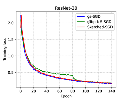
Figure 2: Convergence curves of ResNet-20 trained on Cifar-10 data set with gs-SGD, gTop-k S-SGD and Sketched-SGD with $P=4$.

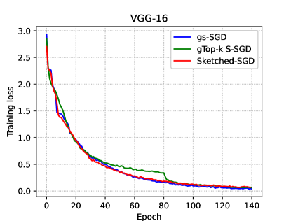
Figure 3: Convergence curves of VGG-16 trained on Cifar-10 data set with gs-SGD, gTop-k S-SGD and Sketched-SGD with $P=4$.

The Convergences of ResNet-20 and VGG-16 models on the Cifar-10 data set are shown in Fig. 2 and Fig. 3. The results show that our gs-SGD basically converges at about 70 epochs, while gTop-$k$ needs about 85 epochs. In other words, the convergence efficiency of gs-SGD on ResNet-20 and VGG-16 is slightly better than that of gTop-$k$, especially before 85 epochs, and almost consistent with the convergence efficiency of original Sketched-SGD.

It can be seen that our algorithm has a better convergence rate than gTop-$k$ algorithm when training the above two models on the Cifar-10 data set, and does not lose the accuracy of the model.

IV-B Time performance analysis

We use the cases of 4 workers to analyze the time performance of gs-SGD. We break down the time of an iteration into three parts: GPU computation time ($t_{compu.}$), local sparsification time ($t_{compr.}$), and communication time ($t_{commu.}$). The results are shown in Fig. 4 and Fig. 5. It is obvious that the communication time of our algorithm is smaller than that of the original Sketched-SGD algorithm, especially on ResNet-20, because the AllReduce time complexity of our algorithm is $O(\log d*\log P)$ while the time complexity of the original Sketched-SGD algorithm is $O(\log d*P)$.

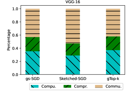
Figure 4: Comparison of the time performance with gs-SGD, Sketched-SGD and gTop-$k$ on VGG-16 with $P=4$.

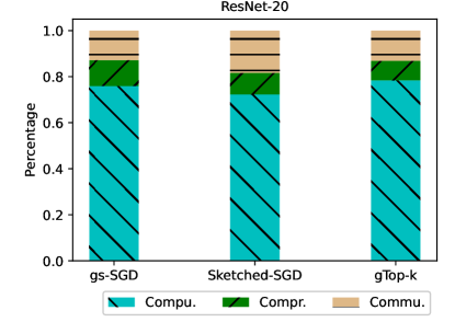
Figure 5: Comparison of the time performance with gs-SGD, Sketched-SGD and gTop-$k$ on ResNet-20 with $P=4$.

IV-C Convergence sensibility to the sparsity

To test the sensibility of convergence of gs-SGD to the sparsity, we run the experiments with different numbers of the parameters $k$ using VGG-16 and ResNet-20 on the Cifar-10 data set on 4 workers. The convergence curves are shown in Fig. 6 and Fig. 7. It can be seen that a very small value of $k$-parameter of 10000 will significantly damage the convergence and accuracy of both models. Therefore, there is a tradeoff between the high compression ratio and a stable convergence speed. In other words, the higher compression ratio would bring lower communication overheads and higher scaling efficiency to a larger cluster. However, this indicates that we need to pay attention to the range of sparsity when training the model to avoid harming the convergence speed and accuracy of the model.

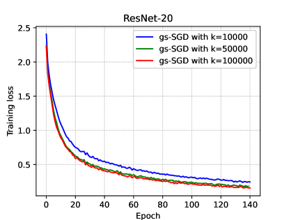
Figure 6: Convergence curves for ResNet-20 trained on Cifar-10 data set with different k on 4 workers.

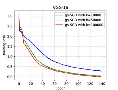
Figure 7: Convergence curves for VGG-16 trained on Cifar-10 data set with different k on 4 workers.

IV-D Scaling efficiency

In terms of scaling efficiency, we evaluate gs-SGD on a cluster with 4 GPU machines that are interconnected with 1 Gbps Ethernet. The summary of the training throughput on different models is shown in Table. II. The experimental results show that our method achieves 1.3—3.1× higher scaling efficiency than gTop-$k$ and 1.1—1.2× improvement than the Sketched-SGD.

TABLE II: THE SYSTEM TRAINING THROUGHPUT^a ON A 4-GPU CLUSTER

Model	gTop-$k$	Sketched-SGD	gs-SGD	$g/k$b	$g/s$c
ResNet-20	804	976	1038	1.3×	1.1×
VGG-16	325	827	1014	3.1×	1.2×

• The throughput is measured with processed images per second.

• indicates the speedup of gs-SGD compared to the gTop-$k$.

• indicates the speedup of gs-SGD compared to Sketched-SGD.

V CONCLUSION

Gradient compression is a promising method to solve the communication bottleneck in synchronous distributed training. In this paper, we propose gs-SGD, which uses $Count-Sketch$ data structure to compress and transmit the gradients between workers, and improves convergence efficiency and system throughput while ensuring the communication complexity is O($\log d*\log P$). We conducted experiments to compare the convergence efficiency and time performance of gs-SGD, gTop-$k$ and Sketched-SGD. The experimental results show that our algorithm has significantly improved the convergence efficiency of training various CNNs, and reduces the communication time ratio among workers. Experiments on different convolutional neural networks, including VGG-16 and ResNet-20, verify that gs-SGD can guarantee convergence efficiency without losing model accuracy. We have conducted experiments on a 4-GPU cluster interconnected with 1Gbps Ethernet to confirm that the training throughput of gs-SGD proposed in this paper increased by 2.2× on average compared with gTop-$k$ S-SGD and 1.15× compared with Sketched-SGD.

For future work, we believe that scenarios with lower bandwidth network, more workers and more complex models are worth experimenting and researching.

References

- [1] Y. LeCun, Y. Bengio, and G. E. Hinton, “Deep learning,” Nat., vol. 521, no. 7553, pp. 436–444, 2015.
- [2] M. Gupta, V. Varma, S. Damani, and K. N. Narahari, “Compression of deep learning models for nlp,” in Proceedings of the 29th ACM International Conference on Information & Knowledge Management, 2020, pp. 3507–3508.
- [3] A. I. Maqueda, A. Loquercio, G. Gallego, N. García, and D. Scaramuzza, “Event-based vision meets deep learning on steering prediction for self-driving cars,” in 2018 IEEECVF Conference on Computer Vision and Pattern Recognition, 2018, pp. 5419–5427.
- [4] K. Simonyan and A. Zisserman, “Very deep convolutional networks for large-scale image recognition,” CoRR, vol. abs/1409.1556, 2015.
- [5] C. Szegedy, V. Vanhoucke, S. Ioffe, J. Shlens, and Z. Wojna, “Rethinking the inception architecture for computer vision,” 2016 IEEE Conference on Computer Vision and Pattern Recognition (CVPR), pp. 2818–2826, 2016.
- [6] J. Redmon, S. Divvala, R. B. Girshick, and A. Farhadi, “You only look once: Unified, real-time object detection,” 2016 IEEE Conference on Computer Vision and Pattern Recognition (CVPR), pp. 779–788, 2016.
- [7] P. Goyal, P. Dollár, R. B. Girshick, P. Noordhuis, L. Wesolowski, A. Kyrola, A. Tulloch, Y. Jia, and K. He, “Accurate, large minibatch sgd: Training imagenet in 1 hour,” ArXiv, vol. abs/1706.02677, 2017.
- [8] O. Russakovsky, J. Deng, H. Su, J. Krause, S. Satheesh, S. Ma, Z. Huang, A. Karpathy, A. Khosla, M. S. Bernstein, A. Berg, and L. Fei-Fei, “Imagenet large scale visual recognition challenge,” International Journal of Computer Vision, vol. 115, pp. 211–252, 2015.
- [9] K. He, X. Zhang, S. Ren, and J. Sun, “Deep residual learning for image recognition,” 2016 IEEE Conference on Computer Vision and Pattern Recognition (CVPR), pp. 770–778, 2016.
- [10] J. Choquette and W. Gandhi, “Nvidia a100 gpu: Performance & innovation for gpu computing,” 2020 IEEE Hot Chips 32 Symposium (HCS), pp. 1–43, 2020.
- [11] N. Jouppi, C. Young, and et al., “In-datacenter performance analysis of a tensor processing unit,” 2017 ACM/IEEE 44th Annual International Symposium on Computer Architecture (ISCA), pp. 1–12, 2017.
- [12] E. Xu, “Huawei launches ascend 910, the world’s most powerful ai processor, and mindspore, an all-scenario ai computing framework,” https://www.huawei.com/en/news/2019/8/huawei-ascend-910-most-powerful-ai-processor, 2019, [Online; accessed 19-July-2021].
- [13] MLCommons, “Mlcommons releases mlperf training v1.0 results,” https://mlcommons.org/en/training-normal-10/r, 2021, [Online; accessed 19-July-2021].
- [14] X. Shi, Z. Chen, H. Wang, D.-Y. Yeung, W.-k. Wong, and W.-c. Woo, “Convolutional lstm network: A machine learning approach for precipitation nowcasting,” in Proceedings of the 28th International Conference on Neural Information Processing Systems - Volume 1, ser. NIPS’15, 2015, p. 802–810.
- [15] M. Li, D. G. Andersen, A. J. Smola, and K. Yu, “Communication efficient distributed machine learning with the parameter server,” in Proceedings of the 27th International Conference on Neural Information Processing Systems, 2014, pp. 19–27.
- [16] Z. Jia, M. Zaharia, and A. Aiken, “Beyond data and model parallelism for deep neural networks.” in Proceedings of Machine Learning and Systems, A. Talwalkar, V. Smith, and M. Zaharia, Eds., 2019, pp. 1–13.
- [17] I. Hubara, M. Courbariaux, D. Soudry, R. El-Yaniv, and Y. Bengio, “Quantized neural networks: Training neural networks with low precision weights and activations,” The Journal of Machine Learning Research, vol. 18, no. 1, pp. 6869–6898, 2017.
- [18] W. Wang and N. Srebro, “Stochastic nonconvex optimization with large minibatches,” in Algorithmic Learning Theory. PMLR, 2019, pp. 857–882.
- [19] Y. You, Z. Zhang, C.-J. Hsieh, J. Demmel, and K. Keutzer, “Imagenet training in minutes,” in Proceedings of the 47th International Conference on Parallel Processing, 2018, pp. 1–10.
- [20] X. Jia, S. Song, W. He, Y. Wang, H. Rong, F. Zhou, L. Xie, Z. Guo, Y. Yang, L. Yu et al., “Highly scalable deep learning training system with mixed-precision: Training imagenet in four minutes,” arXiv preprint arXiv:1807.11205, 2018.
- [21] Y. Lin, S. Han, H. Mao, Y. Wang, and W. Dally, “Deep gradient compression: Reducing the communication bandwidth for distributed training,” ICLR, 2018.
- [22] N. Ivkin, D. Rothchild, E. Ullah, V. Braverman, I. Stoica, and R. Arora, “Communication-efficient distributed sgd with sketching,” in NeurIPS, 2019.
- [23] S. Shi, Q. Wang, K. Zhao, Z. Tang, Y. Wang, X. Huang, and X. Chu, “A distributed synchronous sgd algorithm with global top-k sparsification for low bandwidth networks,” 2019 IEEE 39th International Conference on Distributed Computing Systems (ICDCS), pp. 2238–2247, 2019.
- [24] D. Alistarh, T. Hoefler, M. Johansson, S. Khirirat, N. Konstantinov, and C. Renggli, “The convergence of sparsified gradient methods,” in NeurIPS, 2018.
- [25] S. Shi, K. Zhao, Q. Wang, Z. Tang, and X. Chu, “A convergence analysis of distributed sgd with communication-efficient gradient sparsification,” in Twenty-Eighth International Joint Conference on Artificial Intelligence IJCAI-19, 2019.
- [26] M. Yu, Z. Lin, K. Narra, S. Li, Y. Li, N. S. Kim, A. Schwing, M. Annavaram, and S. Avestimehr, “Gradiveq: Vector quantization for bandwidth-efficient gradient aggregation in distributed cnn training,” in Proceedings of the 32nd International Conference on Neural Information Processing Systems, ser. NIPS’18, 2018, p. 5129–5139.
- [27] T. Vogels, S. P. R. Karimireddy, and M. Jaggi, “Powersgd: Practical low-rank gradient compression for distributed optimization,” in NeurIPS, 2019.
- [28] S. Wang, A. Pi, and X. Zhou, “Scalable distributed dl training: Batching communication and computation,” in AAAI, 2019.
- [29] S. Shi, Q. Wang, X. Chu, B. Li, Y. Qin, R. Liu, and X. Zhao, “Communication-efficient distributed deep learning with merged gradient sparsification on gpus,” IEEE INFOCOM 2020 - IEEE Conference on Computer Communications, pp. 406–415, 2020.
- [30] F. Seide, H. Fu, J. Droppo, G. Li, and D. Yu, “1-bit stochastic gradient descent and its application to data-parallel distributed training of speech dnns,” in INTERSPEECH, 2014.
- [31] J. Bernstein, Y.-X. Wang, K. Azizzadenesheli, and A. Anandkumar, “signsgd: compressed optimisation for non-convex problems,” in ICML, 2018.
- [32] F. Faghri, I. Tabrizian, I. Markov, D. Alistarh, D. M. Roy, and A. Ramezani-Kebrya, “Adaptive gradient quantization for data-parallel sgd,” ArXiv, vol. abs/2010.12460, 2020.
- [33] C.-Y. Chen, J. Choi, D. Brand, A. Agrawal, W. Zhang, and K. Gopalakrishnan, “Adacomp : Adaptive residual gradient compression for data-parallel distributed training,” in AAAI, 2018.
- [34] A. F. Aji and K. Heafield, “Sparse communication for distributed gradient descent,” Proceedings of the 2017 Conference on Empirical Methods in Natural Language Processing, 2017.
- [35] M. Charikar, K. C. Chen, and M. Farach-Colton, “Finding frequent items in data streams,” in ICALP, 2002.
- [36] D. Rothchild, A. Panda, E. Ullah, N. Ivkin, I. Stoica, V. Braverman, J. E. Gonzalez, and R. Arora, “Fetchsgd: Communication-efficient federated learning with sketching,” in ICML, 2020.
- [37] E. Chan, M. Heimlich, A. Purkayastha, and R. V. D. Geijn, “Collective communication: theory, practice, and experience,” Concurrency and Computation: Practice and Experience, vol. 19, 2007.
- [38] R. Thakur, R. Rabenseifner, and W. Gropp, “Optimization of collective communication operations in mpich,” The International Journal of High Performance Computing Applications, vol. 19, pp. 49 – 66, 2005.
- [39] “Open mpi:,” Parallel Processing Letters, vol. 17, no. 01, pp. 79–88, 2008.
- [40] NCCL, “Nvidia collective communication library,” https://docs.nvidia.com/deeplearning/nccl/user-guide/docs/index.html, 2020, [Online; accessed 16-July-2021].