Pole analysis on the doubly charmed meson in $D^{0}D^{0}\pi^{+}$ mass spectrum

Abstract

In this paper we study the scattering amplitudes of $D^{0}D^{0}\pi^{+}$-$D^{*+}D^{0}$ coupled channels based on $K$-matrix within the Chew-Mandelstam formalism. The $D^{0}D^{0}\pi^{+}$ invariant mass spectrum of LHCb is fitted and the pole parameters of the $T_{cc}^{+}$ are extracted. The analysis of pole behavior suggests that the $T_{cc}^{+}$ may originate from a $D^{*+}D^{0}$ virtual state and is formed as a result of an interplay between an attractive interaction between $D^{0}$ and $D^{*+}$ and coupling to $D^{0}D^{0}\pi^{+}$ channel.

Introduction.– For over half a century the quark model served as the fundamental template for constructing hadrons Gell-Mann (1964); Zweig (1964). Dozens of known hadrons can be classified according to this model with three quarks in a baryon and a quark-antiquark pair in a meson. However, the requirement of color neutrality alone does not preclude existence of more complicated structures, including, for example tetraquarks and pentaquarks. In the last twenty years several candidates for such multi-quark hadrons, specifically containing heavy quarks, have been observed by the Belle, BaBar, BESIII, D0, CDF, CMS, and LHCb experimentsChoi et al. (2003); Aaltonen et al. (2009); Bondar et al. (2012); Ablikim et al. (2013a); Liu et al. (2013); Ablikim et al. (2013b); Abazov et al. (2014); Chatrchyan et al. (2014); Aaij et al. (2017, 2020a, 2020b). Significant number of these states are found lying close to various thresholds for decays into non-exotic hadrons. For example the $X(3872)$ discovered by Belle Choi et al. (2003) is in a mass region that is not expected to host a quark model-like charmonium state, but it is only $\sim 1\mbox{ MeV}$ away from the $D\bar{D}^{*}$ threshold. Proximity to this threshold makes it likely to be a $D\bar{D^{*}}$ molecule Guo et al. (2018); Liu et al. (2019); Brambilla et al. (2020). Recently, the LHCb Collaboration announced observation of another $X$-like candidate, this time however, containing two charm quarks instead of a charm-anti-charm pair, labeled $T_{cc}^{+}$ Aaij et al. (2021a, b). The $T_{cc}^{+}$ was observed, with a $21.7\sigma$ significance, in the $D^{0}D^{0}\pi^{+}$ invariant mass spectrum near threshold, aka. with the mass close to the $X(3872)$, $M_{T_{cc}^{+}}-(M_{D^{*+}}+M_{D^{0}})=-237\pm 61~{}keV/c^{2}$ and width, $\Gamma_{T_{cc}^{+}}=410\pm 165~{}keV$. Because two charm quarks alone cannot form a color singlet hadron, if confirmed, the $T_{cc}^{+}$ would be a clear evidence of a multi-quark hadron. The small width indicates that there could be a pole in the relevant partial wave close to the $D^{0}D^{*+}$ threshold, However, since $D^{*}$ decays to $D\pi$, rescattering between $D^{0}D^{0}\pi^{+}$ and $D^{0}D^{*+}$ should be taken into account in determining the pole parameters Dai et al. (2015); Kang et al. (2014); Dai and Pennington (2014a); Danilkin et al. (2015); Chen et al. (2017); Yao et al. (2021).

There have been some theoretical studies for the $T_{cc}^{+}$, see e.g.Agaev et al. (2021); Feijoo et al. (2021); Qin et al. (2021); Li et al. (2021); Dong et al. (2021); Ling et al. (2021). In this note we use effective range approximation and consider the coupled amplitudes for production of $D^{0}D^{0}\pi^{+}$ and $D^{*+}D^{0}$ final states. By fitting to the line shape we obtain a solution for the production amplitude which enables analytical continuation to the complex energy plane where we extract the pole parameters. Finally, by analyzing the pole position we speculate on the possible nature of the $T_{cc}^{+}$ peak.

Formalism.– We need analytical amplitudes to describe the $D^{0}D^{0}\pi^{+}$ invariant mass spectrum in order to obtain accurate pole information. The $T_{cc}^{+}$ is found in the $D^{0}D^{0}\pi^{+}$ invariant mass spectrum near the $D^{*+}D^{0}$ threshold of 3875.09 MeV. One also notices that the branching ratio of $D^{*+}\to D^{0}\pi^{+}$ is $67.7\pm 0.5\%$ Zyla et al. (2020). The $D^{*}$ and $D\pi$ are physically two different states. The former is a resonance (presumably a $q\bar{q}$ bound state in quenched QCD) and the later is in a two-hadron continuum. The two are distinguished, for example by the value of the corresponding thresholds, which is relevant given the proximity of the $T_{cc}$ to the $DD\pi$ threshold.

Hence it is natural to consider the $D^{0}D^{0}\pi^{+}$-$D^{0}D^{*+}$ coupled channels. The analytical coupled channel amplitudes near threshold can be parametrized using a real, symmetric $2\times$2 $K$-matrix to describe the analytical part of the inverse amplitudes,

$$T^{-1}(s)=K^{-1}(s)-C(s)\,,$$ (1)

The matrix elements $C_{i}(s)$ of the diagonal $2\times 2$ Chew-Mandelstam (CM) function Chew and Mandelstam (1960); Edwards and Thomas (1980); Kuang et al. (2020), $C(s)=C_{i}(s)\delta_{i,j}$ contain the right hand cuts starting at the the thresholds, $s_{th,i}=(M_{i}+m_{i})^{2}$. Here the masses are $M_{1}=M_{D^{0}}+m_{\pi^{+}}$, $m_{1}=M_{D^{0}}$, and $M_{2}=M_{D^{*+}}$, $m_{2}=M_{D^{0}}$ for the $D^{0}D^{0}\pi^{+}$ and $D^{0}D^{*+}$ channels, respectively. Note that the $D^{0}\pi^{+}$ system is treated as an isobar of spin-1 and therefore the $T$ describes $S$-wave amplitudes. The CM function,

$$C_{i}(s)=\frac{s}{\pi}\int_{s_{th_{i}}}^{\infty}ds^{\prime}\frac{\rho_{i}(s^{\prime})}{s^{\prime}(s^{\prime}-s)},$$ (2)

is defined by the (quasi)two-body $S$-wave phase space factor, $ImC_{i}(s)=\rho_{i}(s)=\lambda^{1/2}(s,M_{i}^{2},m_{i}^{2})/s$, explicitly,

$$C_{i}(s;M_{i},m_{i})=\left[\frac{M_{i}^{2}-m_{i}^{2}}{\pi s}-\frac{M_{i}^{2}+m_{i}^{2}}{\pi(M_{i}^{2}-m_{i}^{2})}\right]\ln\left(\frac{m_{i}}{M_{i}}\right)$$

$$+\frac{1}{\pi}+\frac{\rho_{i}(s)}{\pi}\ln\left[\frac{\sqrt{s_{th_{i}}-s}-\sqrt{(M_{i}-m_{i})^{2}-s}}{\sqrt{s_{th_{i}}-s}+\sqrt{(M_{i}-m_{i})^{2}-s}}\right].$$ (3)

With the threshold singularities accounted for by $C(s)$, the $K$-matrix is analytical in the vicinity at thresholds and in the effective range approximation it as approximated by a matrix of constants.

In the notation of Au et al. (1987); Dai and Pennington (2014b) the $s$-dependence of production amplitude for the processes $pp\to D^{0}D^{0}\pi^{+}+X$ and $pp\to D^{0}D^{*+}+X$, can be represented by a two-dimensional vector

$$F_{i}(s) = \sum_{k=1}^{2}\alpha_{k}(s)T_{ki}(s)\;.$$ (4)

where $\alpha_{i}(s)$ are regular functions of $s$ on the physical cut. Since the range of invariant mass is small, with $\Delta\sqrt{s}<<O(100\mbox{ MeV})$, we can safely ignore any variation in $s$ of the production amplitudes, $\alpha_{i}(s)$ and also approximate them by constants. Finally, the measured yield is proportional to the differential cross section and given by

$$\frac{dY_{1}}{d\sqrt{s}}=\;Np_{1}|F_{1}|^{2}.$$ (5)

Here $p_{1}=\lambda(s,M_{1}^{2},m^{2}_{1})/2\sqrt{s}$ is the magnitude of the momentum of the $\pi^{+}$ in the center of mass frame. Since the overall number of events is fitted we can absorb $\alpha_{1}$ into the normalization factor $N$ and thus we set $\alpha_{1}=1$.

Fit results and discussion.– We fit the amplitudes to the $D^{0}D^{0}\pi^{+}$ invariant mass spectrum Aaij et al. (2021a, b) using MINUIT James and Roos (1975). One needs to consider the resolution for the $D^{0}D^{0}\pi^{+}$ mass. Here we follow the experiment Aaij et al. (2021b), convolute Eq. (6) with the resolution function. For a data point with mass $E_{i}$, we get the Yields for the bin:

$$\frac{{\rm Yields}}{{\rm\Delta E}} = \int_{(E_{i}-\Delta E/2)^{2}}^{(E_{i}+\Delta E/2)^{2}}ds~{}\frac{Np_{1}|F_{1}|^{2}}{2\Delta E\sqrt{s}}$$ (6)

$$\left\{\sum_{j=1}^{2}\beta_{j}\exp\left[-\frac{1}{2}\left(\frac{\sqrt{s}-E_{i}}{\sigma_{j}}\right)^{2}\right]\right\}\,,$$

where $\Delta E$ is the bin width, $\beta_{1}=0.778$, $\beta_{2}=0.222$, $\sigma_{1}=1.05\times 263$ keV, and $\sigma_{2}=2.413\times\sigma_{1}$ Aaij et al. (2021b). We find a unique solution with desired physical properties. The parameters of the fit are given in Table 1, and correspond to $\chi^{2}_{\rm d.o.f}=0.92$. Notice that the error of the parameters from MINUIT is much smaller than that from bootstrap Efron (1979), which is done by varying the data with experimental uncertainty multiplying a normal distribution function.

$K_{11}=-0.01204\pm 0.00691^{+0.03280}_{-0.07039}$

$K_{12}=K_{21}=0.5080\pm 0.0025^{+0.0348}_{-0.0700}$

$K_{22}=1.4447\pm 0.0015^{+0.0235}_{-0.0477}$

$\alpha_{2}=-0.3024\pm 0.0016^{+0.0261}_{-0.0583}$

$N_{a}=1434.0\pm 129.8^{+662.0}_{-964.8}\mbox{ GeV}^{-2}$

$N_{b}=516.0\pm 49.3^{+225.6}_{-363.4}\mbox{ GeV}^{-2}$

$\chi^{2}_{{\rm d.o.f}}$=0.92

Table 1: Parameters of the best fit, as explained in the text. The $K$-matrix elements and production parameters, $\alpha_{i}$ are dimensionless. The first uncertainty of the parameters is given from MINUIT, and the second (up and down) uncertainty is from bootstrap within 2$\sigma$. $N_{a}$ is the normalization factor for the data in the full range, while $N_{b}$ is for the data in the region of $T_{cc}^{+}$. The correlation matrix is given in supplemental material.

The comparison between the data and the model is shown in Fig. 1.

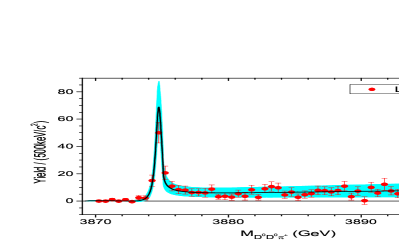
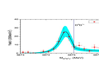
Figure 1: The clear line shape from our solutions. The data points of $D^{0}D^{0}\pi^{+}$ invariant mass spectrum are superimposed. The cyan bands are taken from bootstrap method within 2$\sigma$.

As can be seen, our amplitudes fit the data rather well. To study the resonance we also enlarge the plot of our solution around the $T_{cc}^{+}$, multiplying $N_{b}$ instead of $N_{a}$ in Eq. (5), as shown in the bottom graph in Fig. 1. Once the $D^{0}D^{0}\pi^{+}$-$D^{0}D^{*+}$ amplitudes are determined on the real axis they can be analytically continued to extract the information about the singularities located on the nearby Riemann sheets (RS). These are reached from the real $s$-axis though the unitary cuts of the $C_{i}(s)$ functions. Near the pole $s_{R}$ residues/couplings in $n$-th RS are computed from

$$T^{n}_{ij}(s)\simeq\frac{g^{n}_{i}g^{n}_{j}}{s_{R}^{n}-s}\,.$$ (7)

We find a single pole on RS-II and the pole parameters are given in Table 2.

pole location (MeV)	$g^{II}_{D^{0}D^{0}\pi^{+}}=|g|e^{i\varphi}$		$g^{II}_{D^{0}D^{*+}}=|g|e^{i\varphi}$
	$|g_{1}|$ (GeV)	$\varphi_{1}$ (∘)	$|g_{2}|$ (GeV)	$\varphi_{2}$ (∘)
$3874.74^{+0.11}_{-0.04}-i~{}0.30^{+0.05}_{-0.09}$	$0.22^{+0.03}_{-0.04}$	$9^{+11}_{-5}$	$0.69^{+0.04}_{-0.02}$	$10^{+11}_{-5}$

Table 2: The pole location and its residues (both magnitude and phase) from our fit, in RS-II.

Here we follow the standard labeling of the sheets, e.g. the second sheet is reached from the physical region by moving into the lower complex plane between two thresholds Frazer and Hendry (1964). The uncertainty of the pole parameters come from bootstrap within 2$\sigma$.

Notice that in the bootstrap method, where the data points are varied randomly, all the poles are located in RS-II. Since $|g_{2}|>|g_{1}|$ it appears that $T_{cc}^{+}$ couples more strongly (roughly a factor of three) to the $D^{0}D^{*+}$ channel than to the $D^{0}D^{0}\pi^{+}$ channel. This supports the hypothesis that $T_{cc}^{+}$ is a composite object dominated by the $D^{0}D^{*+}$ component.

The trajectory of the pole on the second Riemann sheet is studied by varying $\lambda$ which is introduced to modify the strength of coupling between the two channels, $K_{12}(s)\to\lambda K_{12}(s)$, so that $\lambda=1$ corresponds to the physical amplitude while for $\lambda=0$, Eq.(1) represents two uncoupled channels. As a function of $\lambda$ the pole trajectory is shown in Fig. 2.

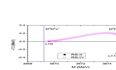
Figure 2: The trajectories of pole locations by varying $\lambda$. The black filled circles are the poles in the second Riemann sheet, $1\geq\lambda\geq 0.88$, and the magenta open circles are the poles in the fourth Riemann sheet, $0.87\geq\lambda\geq 0$, respectively. The step of $\Delta\lambda$ is 0.01.

As $\lambda$ decreases, the pole moves upwards from the lower half $\sqrt{s}$-plane of RS-II to the upper half plane of RS-IV, crossing the real axis above the second (heavier) $D^{0}D^{*+}$ threshold. This does not violate unitarity since while moving from the second to the fourth sheet the pole never crosses the physical region. As this happens the resonance bump seen on the real axis between thresholds moves towards the heavier threshold and as the pole enters the fourth sheet it becomes a cusp. As $\lambda$ is decreased further the poles moves below the lower threshold and into the real axis. Finally it reaches the mass just $\sim 0.21\mbox{ MeV}$ above the $D^{0}D^{0}\pi^{+}$ threshold. Notice that at the end of the trajectory with $\lambda=0$, corresponding to the $D^{0}D^{*+}$ single channel, the pole in the real axis below threshold is a virtual state. This implies that in the absence of channel coupling the $D^{0}D^{*+}$ system may not be sufficiently attractive to produce a molecule. If so the $T_{cc}^{+}$ is not a true bound state (a pole remaining on the second sheet) but an effect of a complicated interplay of weak attraction and channel interactions. This behaviour is similar to that of the $P_{c}(4312)$, which was found to be likely an effect of weak interaction between $\Sigma_{C}^{+}\bar{D}^{0}$ and coupling the the $J/\psi p$ channel Fernández-Ramírez et al. (2019).

To further assess systematic uncertainties we include higher order terms in the effective range expansion. This slightly improves the fit quality but does not qualitatively change the amplitudes in the vicinity of the $T_{cc}^{+}$. In yet another check, we include the fit to the data without the resolution function. In this case, still only one pole is found in the RS-II, $3874.75^{+0.12}_{-0.06}-i~{}0.34^{+0.06}_{-0.12}$ MeV, with the residues of $|g_{1}|=0.23^{+0.03}_{-0.04}$ GeV and $|g_{2}|=0.70^{+0.03}_{-0.03}$ GeV. Quite the same as what is found in Table 2.

Role of the $D^{*}$ width.– Since $D^{*+}$ is unstable its contribution to the spectral function corresponds to a branch cut (below the real axis) and not a pole. To account for that we modify the Chew-Mandelstam $C_{2}$ accordingly Basdevant and Berger (1979):

$$C_{2}(s)\to\frac{1}{\pi}\int_{s_{tr,D\pi}}^{\infty}ds^{\prime}C(s;\sqrt{s^{\prime}},m_{2}){\rm Im}f_{D\pi}(s^{\prime})$$ (8)

with $s_{th,D\pi}=(M_{D^{0}}+m_{\pi}^{+})^{2}$ being the threshold for the reaction $D^{0}\pi^{+}\to D^{*+}\to D^{0}\pi^{+}$ and $f_{D\pi}(s)=D^{-1}(s)$, the scattering amplitude in the single resonance approximation, with $D(s)=\tilde{M}^{2}-s-\Sigma(s)$, and $\Sigma(s)=g^{2}(s-s_{th,D\pi})C(s;M_{2},m_{2})$ so that the imaginary part, ${\rm Im}\Sigma(s)=g^{2}(s-s_{th,D\pi})\rho_{2}(s)$ is the energy dependent width corresponding to the $P$-wave decay of the $D^{*+}\to D^{0}\pi^{+}$. With the parameters $g=0.4451$ and $\tilde{M}=2010.77$ MeV the amplitude $f$ reproduces the line shape of the $D^{*}$ correspond to a Breit-Wigner resonance with pole at $M_{D^{*+}}-i\Gamma_{M_{D^{*+}}}/2=2010.26-i0.04$ MeV. With this modification of $C_{2}(s)$, we fit the coupled channel amplitudes again, convoluting with Eq. (6) with the resolution function, and find a rather similar solution to the previous one. A pole is found in RS-II with $3874.76^{+0.08}_{-0.04}-i~{}0.26^{+0.02}_{-0.09}$ MeV, and the residues are extracted as $|g_{1}|=0.21^{+0.01}_{-0.04}$ GeV and $|g_{2}|=0.71^{+0.02}_{-0.02}$ GeV. The pole trajectory is the same as what we found in Fig.2, with only the pole moves towards but not reach the real axis. Also the destination of the pole (with $\lambda=0$) being roughly 2.6 MeV above the $D^{0}D^{0}\pi^{+}$ threshold. These support the conclusion before.

Summary.– In this letter we performed amplitude analysis on the invariant mass spectrum of $D^{0}D^{0}\pi^{+}$. The $D^{0}D^{0}\pi^{+}$  -  $D^{0}D^{*+}$ coupled channel scattering amplitude is constructed using a K-matrix within the Chew-Mandelstam formalism. Then we apply the Au-Morgan-Pennington method to study the final state interactions for the invariant mass spectrum of $D^{0}D^{0}\pi^{+}$. A high quality fit to the experiment data of LHCb Aaij et al. (2021a, b) is obtained. We find a pole in the second Riemann sheet for the $T_{cc}^{+}$, with the pole location $3874.74^{+0.11}_{-0.04}-i~{}0.30^{+0.05}_{-0.09}$ MeV. By reducing the strength of inelastic channels we obtain the pole trajectory that suggests $T_{cc}^{+}$ might be a $D^{0}D^{*+}$ virtual state. Precise measurements of the line shape would be need to further reduce theoretical uncertainties.

Acknowledgements.– We thank C. Fernández-Ramírez for helpful discussions on bootstrap method. This work is supported by Joint Large Scale Scientific Facility Funds of the National Natural Science Foundation of China (NSFC) and Chinese Academy of Sciences (CAS) under Contract No.U1932110, National Natural Science Foundation of China with Grants No.11805059, No.11805012, No.11675051 and No.12061141006, Fundamental Research Funds for the central universities of China, and U.S. Department of Energy Grants No. DE-AC05-06OR23177 and No. DE-FG02- 87ER40365.

Appendix A Supplemental material

Different fits.– To study systematic uncertainties we vary the number of parameters in the $K$-matrix,

$$K^{ij}(s) = \sum_{l}\frac{f^{i}_{l}f^{j}_{l}}{(s_{l}-s)}+\sum_{n=0}c^{ij}_{n}(\frac{s}{s_{th2}}-1)^{n}\;.$$ (A)

Near threshold the $K$-matrix can be simplified to effective range formula so that $f^{i}_{l}$, and all higher order polynomials, $c^{ij}_{n\geq 2}$ given in Eq.(A) are set to zero. In an alternative fit, which we refer to as Fit A, we add one more term, proportional to $c^{ij}_{1}$, in each element of the $K$. Thus Fit A, has six parameters to parametrize the $T$-matrix, compared to three used in the nominal fit. To reduce the correlation between parameters, in Fit A we use the same normalization factors as obtained from the nominal fit presented in the paper. Furthermore, to investigate the effects of resolution, in Fit B we use the nominal model removing the smearing. The parameters and $\chi^{2}/d.o.f$ of these fits are summarized in Table A.

	Fit A	Fit B
$c^{11}_{0}$	$-0.1067\pm 0.0170^{+0.1079}_{-0.0415}$	$0.007905\pm 0.006404^{+0.034727}_{-0.082606}$
$c^{11}_{1}$	$10.5612\pm 5.1641^{+10.4981}_{-4.0526}$	$\cdots$
$c^{12}_{0}$	$0.5080$	$0.5315\pm 0.0025^{+0.0320}_{-0.0666}$
$c^{12}_{1}$	$-15.3292\pm 3.2335^{+17.2790}_{-5.1199}$	$\cdots$
$c^{22}_{0}$	$1.4550\pm 0.0021^{+0.0145}_{-0.0054}$	$1.4271\pm 0.0016^{+0.0222}_{-0.0491}$
$c^{22}_{1}$	$8.3280\pm 5.6488^{+49.6034}_{-17.3702}$	$\cdots$
$\alpha_{2}$	$-0.2866\pm 0.0027^{+0.0174}_{-0.0062}$	$-0.3215\pm 0.0015^{+0.0270}_{-0.0606}$
$N_{a}$ ($\mbox{ GeV}^{-2}$)	$1434.0$	$1339.6\pm 117.7^{+639.1}_{-952.5}$
$N_{b}$ ($\mbox{ GeV}^{-2}$)	$516.0$	$568.5\pm 52.0^{+268.4}_{-394.8}$
$\chi^{2}_{{\rm d.o.f}}$	0.86	0.95

Table A: Results of Fits A and B, as explained in the text. The $c^{ij}_{0}$ is dimensionless and the $c^{ij}_{1}$ is in unit of GeV^-2. The uncertainty of the parameters is given from MINUIT, and the upper and lower errors are taken from Bootstrap method.

The quality of all fits are similar. For completeness, in Table B we give the correlation matrix between the parameters of the nominal fit.

	$K_{11}$	$K_{12}$	$K_{22}$	$\alpha_{2}$	$N_{a}$
$K_{11}$	1.000	0.422	-0.067	-0.580	-0.082
$K_{12}$	0.422	1.000	-0.100	-0.628	-0.095
$K_{22}$	-0.067	-0.100	1.000	0.671	0.018
$\alpha_{2}$	-0.580	-0.628	0.671	1.000	-0.012
$N_{a}$	-0.082	-0.095	0.018	0.012	1.000

Table B: Correlation coefficients between parameters of the nominal fit using bootstrap. $N_{b}$ is rescaling from $N_{a}$ and thus we do not list the correlation coefficients related to it.

The larges deviation with respect to the nominal (referred to in the figures as Sol. I) is observed in Fit B. In Fit B, the peak appears to be a bit lower compared with the unresolved data. The mass distributions from the fits are shown in Fig. A and in Table C we give the $T_{cc}^{+}$ pole parameters.

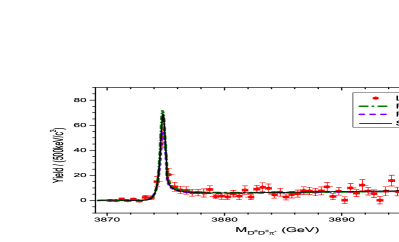
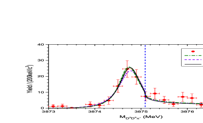
Figure A: Line shapes from our solutions. The olive dash-dotted lines are for Fit A and the violet dashed lines are for Fit B.

Cases	pole location (MeV)	$g^{II}_{D^{0}D^{0}\pi^{+}}=|g|e^{i\varphi}$		$g^{II}_{D^{0}D^{*+}}=|g|e^{i\varphi}$
		$|g_{1}|$ (GeV)	$\varphi_{1}$ (∘)	$|g_{2}|$ (GeV)	$\varphi_{2}$ (∘)
Fit A	$3874.71^{+0.11}_{-0.05}-i~{}0.28^{+0.04}_{-0.10}$	$0.21^{+0.04}_{-0.04}$	$9^{+11}_{-9}$	$0.69^{+0.07}_{-0.12}$	$9^{+11}_{-8}$
Fit B	$3874.75^{+0.12}_{-0.06}-i~{}0.34^{+0.06}_{-0.12}$	$0.23^{+0.03}_{-0.04}$	$10^{+13}_{-9}$	$0.70^{+0.03}_{-0.03}$	$11^{+13}_{-8}$

Table C: The pole locations and their residues (both magnitudes and phases) from our fits, in RS-II.

As shown in Fig. B, the pole trajectories of Fits A and B are very similar to that of the nominal fit.

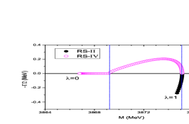
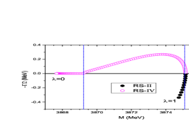
Figure B: The trajectories of pole locations by varying $\lambda$. The black filled circles represent for the poles in the second Riemann sheet, and the magenta open circles represent for the poles in the fourth Riemann sheet. The step of $\Delta\lambda$ is 0.01. The left graph corresponds to Fit A, and the right one to Fit B.

References

- Gell-Mann (1964) M. Gell-Mann, Phys. Lett. 8, 214 (1964).
- Zweig (1964) G. Zweig, “An SU(3) model for strong interaction symmetry and its breaking. CERN Report No. 8182/TH.401.” (1964).
- Choi et al. (2003) S. K. Choi et al. (Belle), Phys. Rev. Lett. 91, 262001 (2003), arXiv:hep-ex/0309032 .
- Aaltonen et al. (2009) T. Aaltonen et al. (CDF), Phys. Rev. Lett. 102, 242002 (2009), arXiv:0903.2229 [hep-ex] .
- Bondar et al. (2012) A. Bondar et al. (Belle), Phys. Rev. Lett. 108, 122001 (2012), arXiv:1110.2251 [hep-ex] .
- Ablikim et al. (2013a) M. Ablikim et al. (BESIII), Phys. Rev. Lett. 110, 252001 (2013a), arXiv:1303.5949 [hep-ex] .
- Liu et al. (2013) Z. Q. Liu et al. (Belle), Phys. Rev. Lett. 110, 252002 (2013), [Erratum: Phys.Rev.Lett. 111, 019901 (2013)], arXiv:1304.0121 [hep-ex] .
- Ablikim et al. (2013b) M. Ablikim et al. (BESIII), Phys. Rev. Lett. 111, 242001 (2013b), arXiv:1309.1896 [hep-ex] .
- Abazov et al. (2014) V. M. Abazov et al. (D0), Phys. Rev. D 89, 012004 (2014), arXiv:1309.6580 [hep-ex] .
- Chatrchyan et al. (2014) S. Chatrchyan et al. (CMS), Phys. Lett. B 734, 261 (2014), arXiv:1309.6920 [hep-ex] .
- Aaij et al. (2017) R. Aaij et al. (LHCb), Phys. Rev. Lett. 118, 022003 (2017), arXiv:1606.07895 [hep-ex] .
- Aaij et al. (2020a) R. Aaij et al. (LHCb), Phys. Rev. Lett. 125, 242001 (2020a), arXiv:2009.00025 [hep-ex] .
- Aaij et al. (2020b) R. Aaij et al. (LHCb), Phys. Rev. D 102, 112003 (2020b), arXiv:2009.00026 [hep-ex] .
- Guo et al. (2018) F.-K. Guo, C. Hanhart, U.-G. Meißner, Q. Wang, Q. Zhao, and B.-S. Zou, Rev. Mod. Phys. 90, 015004 (2018), arXiv:1705.00141 [hep-ph] .
- Liu et al. (2019) Y.-R. Liu, H.-X. Chen, W. Chen, X. Liu, and S.-L. Zhu, Prog. Part. Nucl. Phys. 107, 237 (2019), arXiv:1903.11976 [hep-ph] .
- Brambilla et al. (2020) N. Brambilla, S. Eidelman, C. Hanhart, A. Nefediev, C.-P. Shen, C. E. Thomas, A. Vairo, and C.-Z. Yuan, Phys. Rept. 873, 1 (2020), arXiv:1907.07583 [hep-ex] .
- Aaij et al. (2021a) R. Aaij et al. (LHCb), (2021a), arXiv:2109.01038 [hep-ex] .
- Aaij et al. (2021b) R. Aaij et al. (LHCb), (2021b), arXiv:2109.01056 [hep-ex] .
- Dai et al. (2015) L. Y. Dai, M. Shi, G.-Y. Tang, and H. Q. Zheng, Phys. Rev. D 92, 014020 (2015), arXiv:1206.6911 [hep-ph] .
- Kang et al. (2014) X.-W. Kang, B. Kubis, C. Hanhart, and U.-G. Meißner, Phys. Rev. D 89, 053015 (2014), arXiv:1312.1193 [hep-ph] .
- Dai and Pennington (2014a) L.-Y. Dai and M. R. Pennington, Phys. Rev. D 90, 036004 (2014a), arXiv:1404.7524 [hep-ph] .
- Danilkin et al. (2015) I. V. Danilkin, C. Fernández-Ramírez, P. Guo, V. Mathieu, D. Schott, M. Shi, and A. P. Szczepaniak, Phys. Rev. D 91, 094029 (2015), arXiv:1409.7708 [hep-ph] .
- Chen et al. (2017) Y.-H. Chen, M. Cleven, J. T. Daub, F.-K. Guo, C. Hanhart, B. Kubis, U.-G. Meißner, and B.-S. Zou, Phys. Rev. D 95, 034022 (2017), arXiv:1611.00913 [hep-ph] .
- Yao et al. (2021) D.-L. Yao, L.-Y. Dai, H.-Q. Zheng, and Z.-Y. Zhou, Rept. Prog. Phys. 84, 076201 (2021), arXiv:2009.13495 [hep-ph] .
- Agaev et al. (2021) S. S. Agaev, K. Azizi, and H. Sundu, (2021), arXiv:2108.00188 [hep-ph] .
- Feijoo et al. (2021) A. Feijoo, W. H. Liang, and E. Oset, (2021), arXiv:2108.02730 [hep-ph] .
- Qin et al. (2021) Q. Qin, Y.-F. Shen, and F.-S. Yu, Chin. Phys. C 45, 103106 (2021), arXiv:2008.08026 [hep-ph] .
- Li et al. (2021) N. Li, Z.-F. Sun, X. Liu, and S.-L. Zhu, Chin. Phys. Lett. 38, 092001 (2021), arXiv:2107.13748 [hep-ph] .
- Dong et al. (2021) X.-K. Dong, F.-K. Guo, and B.-S. Zou, (2021), 10.1088/1572-9494/ac27a2, arXiv:2108.02673 [hep-ph] .
- Ling et al. (2021) X.-Z. Ling, M.-Z. Liu, L.-S. Geng, E. Wang, and J.-J. Xie, (2021), arXiv:2108.00947 [hep-ph] .
- Zyla et al. (2020) P. A. Zyla et al. (Particle Data Group), PTEP 2020, 083C01 (2020).
- Chew and Mandelstam (1960) G. F. Chew and S. Mandelstam, Phys. Rev. 119, 467 (1960).
- Edwards and Thomas (1980) B. J. Edwards and G. H. Thomas, Phys. Rev. D 22, 2772 (1980).
- Kuang et al. (2020) S.-Q. Kuang, L.-Y. Dai, X.-W. Kang, and D.-L. Yao, Eur. Phys. J. C 80, 433 (2020), arXiv:2002.11959 [hep-ph] .
- Au et al. (1987) K. Au, D. Morgan, and M. Pennington, Phys. Rev. D 35, 1633 (1987).
- Dai and Pennington (2014b) L.-Y. Dai and M. R. Pennington, Phys. Lett. B 736, 11 (2014b), arXiv:1403.7514 [hep-ph] .
- James and Roos (1975) F. James and M. Roos, Comput. Phys. Commun. 10, 343 (1975).
- Efron (1979) B. Efron, Annals Statist. 7, 1 (1979).
- Frazer and Hendry (1964) W. R. Frazer and A. W. Hendry, Phys. Rev. 134, B1307 (1964).
- Fernández-Ramírez et al. (2019) C. Fernández-Ramírez, A. Pilloni, M. Albaladejo, A. Jackura, V. Mathieu, M. Mikhasenko, J. A. Silva-Castro, and A. P. Szczepaniak (JPAC), Phys. Rev. Lett. 123, 092001 (2019), arXiv:1904.10021 [hep-ph] .
- Basdevant and Berger (1979) J. L. Basdevant and E. L. Berger, Phys. Rev. D 19, 239 (1979).