An Operator Splitting View of Federated Learning

Abstract

Over the past few years, the federated learning (FL) community has witnessed a proliferation of new FL algorithms. However, our understating of the theory of FL is still fragmented, and a thorough, formal comparison of these algorithms remains elusive. Motivated by this gap, we show that many of the existing FL algorithms can be understood from an operator splitting point of view. This unification allows us to compare different algorithms with ease, to refine previous convergence results and to uncover new algorithmic variants. In particular, our analysis reveals the vital role played by the step size in FL algorithms. The unification also leads to a streamlined and economic way to accelerate FL algorithms, without incurring any communication overhead. We perform numerical experiments on both convex and nonconvex models to validate our findings.

1 Introduction

The accompanying (moderate) computational power of modern smart devices such as phones, watches, home appliances, cars, etc., and the enormous data accumulated from their interconnected ecosystem have fostered new opportunities and challenges to train/tailor modern deep models. Federated learning (FL), as a result, has recently emerged as a massively distributed framework that enables training a shared or personalized model without infringing user privacy. Tremendous progress has been made since the seminal work of [1], including algorithmic innovations [2, 3, 4, 5, 6, 7, 8], convergence analysis [9, 10, 11, 12, 13], personalization [14, 15, 16, 17, 18], privacy protection [19, 20], model robustness [21, 22, 23, 24], fairness [25, 26, 27], standardization [28, 29], applications [30], just to name a few. We refer to the excellent surveys [31, 32, 33] and the references therein for the current state of affairs in FL.

The main goal of this work is to take a closer examination of some of the most popular FL algorithms, including FedAvg [1], FedProx [2], and FedSplit [5], by connecting them with the well-established theory of operator splitting in optimization. In particular, we show that FedAvg corresponds to forward-backward splitting and we demonstrate a trade-off in its step size and number of local epochs, while a similar phenomenon has also been observed in [10, 5, 12, 34]. FedProx, on the other hand, belongs to backward-backward splitting, or equivalently, forward-backward splitting on a related but regularized problem, which has been somewhat overlooked in the literature. Interestingly, our results reveal that the recent personalized model in [15] is exactly the problem that FedProx aims to solve. Moreover, we show that when the step size in FedProx diminishes (sublinearly fast), then it actually solves the original problem, which is contrary to the observation in [5] where the step size is fixed and confirms again the importance of step size in FL.

For FedSplit, corresponding to Peaceman-Rachford splitting [35, 36], we show that its convergence (in theory) heavily hinges on the strong convexity of the objective and hence might be less stable for nonconvex problems.

Inspecting FL through the lens of operator splitting also allows us to immediately uncover new FL algorithms, by adapting existing splitting algorithms. Indeed, we show that Douglas-Rachford splitting [37, 36] (more precisely the method of partial inverse [38]) yields a (slightly) slower but more stable variant of FedSplit, while at the same time shares a close connection to FedProx: the latter basically freezes the update of a dual variable in the former. We also propose FedRP by combining the reflector in FedSplit and the projection (averaing) in FedAvg and FedProx, and extend an algorithm of [39]. We improve the convergence analysis of FedRP and empirically demonstrate its competitiveness with other FL algorithms. We believe these results are just the tip of the ice-berg and much more progress can now be expected: the marriage between FL and operator splitting simply opens a range of new possibilities to be explored.

Our holistic view of FL algorithms suggests a very natural unification, building on which we show that the aforementioned algorithms reduce to different parameter settings in a grand scheme. We believe this is an important step towards standardizing FL from an algorithmic point of view, in addition to standard datasets, models and evaluation protocols as already articulated in [28, 29]. Our unification also allows one to compare and implement different FL algorithms with ease, and more importantly to accelerate them in a streamlined and economic fashion. Indeed, for the first time we show that Anderson-acceleration [40, 41], originally proposed for nonlinear fixed-point iteration, can be adapted to accelerate existing FL algorithms and we provide practical implementations that do not incur any communication overhead. We perform experiments on both convex and nonconvex models to validate our findings, and compare the above-mentioned FL algorithms on an equal footing.

We proceed in §2 with some background introduction. Our main contributions are presented in §3, where we connect FL with operator splitting, shed new insights on existing algorithms, suggest new algorithmic variants and refine convergence analysis, and in §4, where we present a unification of current algorithms and propose strategies for further acceleration. We conclude in §5 with some future directions. Due to space limit, all proofs are deferred to Appendix C.

2 Background

In this section we recall the federated learning (FL) framework of [1]. We consider $m$ users (edge devices), where the $i$-th user aims at minimizing a function $f_{i}:\mathds{R}^{d}\to\mathds{R},i=1,\ldots,m$, defined on a shared model parameter $\mathbf{w}\in\mathds{R}^{d}$. Typically, each user function $f_{i}$ depends on the respective user’s local (private) data $\mathcal{D}_{i}$. The main goal in FL is to collectively and efficiently optimize individual objectives $\{f_{i}\}$ in a decentralized, privacy-preserving and low-communication way.

Following [1], many existing FL algorithms fall into the natural formulation that optimizes the (arithmetic) average performance:

$$\min_{\mathbf{w}\in\mathds{R}^{d}}\leavevmode\nobreak\ f(\mathbf{w}),\leavevmode\nobreak\ \leavevmode\nobreak\ \mathrm{where}\ \leavevmode\nobreak\ \leavevmode\nobreak\ f(\mathbf{w}):=\sum_{{i}=1}^{m}\lambda_{i}f_{i}(\mathbf{w}).$$ (1)

The weights $\lambda_{i}$ here are nonnegative and w.l.o.g. sum to 1. Below, we assume they are specified beforehand and fixed throughout.

To facilitate our discussion, we recall the Moreau envelope and proximal map of a function $f:\mathds{R}^{d}\to\mathds{R}\cup\{\infty\}$, defined respectively as:

$$\mathsf{M}_{f}^{\eta}(\mathbf{w})=\min_{\mathbf{x}}\leavevmode\nobreak\ \tfrac{1}{2\eta}\|\mathbf{x}-\mathbf{w}\|_{2}^{2}+f(\mathbf{x}),\qquad\mathsf{P}_{f}^{\eta}(\mathbf{w})=\operatorname*{argmin}_{\mathbf{x}}\leavevmode\nobreak\ \tfrac{1}{2\eta}\|\mathbf{x}-\mathbf{w}\|_{2}^{2}+f(\mathbf{x}),$$ (2)

where $\eta>0$ is a parameter acting similarly as the step size. We also define the reflector

$$\mathsf{R}_{f}^{\eta}(\mathbf{w}) =2\mathsf{P}_{f}^{\eta}(\mathbf{w})-\mathbf{w}.$$ (3)

As shown in fig. 1, when $f=\iota_{C}$ is the indicator function of a (closed) set $C\subseteq\mathds{R}^{d}$, $\mathsf{P}_{f}^{\eta}(\mathbf{w})\equiv\mathsf{P}_{C}(\mathbf{w})$ is the usual (Euclidean) projection onto the set $C$ while $\mathsf{R}_{f}^{\eta}(\mathbf{w})\equiv\mathsf{R}_{C}(\mathbf{w})$ is the reflection of $\mathbf{w}$ w.r.t. $C$.

Figure 1: When $f=\iota_{C}$ is the indicator function of a (closed) set $C$, $\mathsf{P}_{f}^{\eta}(\mathbf{w})$ is the Euclidean projection of $\mathbf{w}$ onto the set $C$. Similarly, $\mathsf{R}_{f}^{\eta}(\mathbf{v})$ is the Euclidean reflection of $\mathbf{v}$ w.r.t. the set $C$.

We are now ready to reformulate our main problem of interest (1) in a product space:

$$\min_{\mathsf{w}\in H}\leavevmode\nobreak\ \mathsf{f}(\mathsf{w})=\left\langle\mathbf{1},\mathbf{f}(\mathsf{w})\right\rangle,\leavevmode\nobreak\ \mathrm{where}\ \leavevmode\nobreak\ \mathbf{f}(\mathsf{w}):=\big{(}f_{1}(\mathbf{w}_{1}),\ldots,f_{m}(\mathbf{w}_{m})\big{)},$$ (4)

$\mathbf{1}$ is the vector of all 1s,

$$H:=\{\mathsf{w}=(\mathbf{w}_{1},\ldots,\mathbf{w}_{m})\in\mathds{R}^{dm}:\leavevmode\nobreak\ \mathbf{w}_{1}=\cdots=\mathbf{w}_{m}\}$$ (5)

and we equip with the inner product

$$\left\langle\mathsf{w},\mathsf{z}\right\rangle=\left\langle\mathsf{w},\mathsf{z}\right\rangle_{\bm{\lambda}}:=\sum_{i}\lambda_{i}\mathbf{w}_{i}^{\top}\mathbf{z}_{i}.$$ (6)

Note that the complement $H^{\perp}=\{\mathsf{w}:\sum_{i}\lambda_{i}\mathbf{w}_{i}=\mathbf{0}\}$, and

$$\mathsf{P}_{H}(\mathsf{w})=(\bar{\mathbf{w}},\ldots,\bar{\mathbf{w}}),\leavevmode\nobreak\ \mathrm{where}\ \leavevmode\nobreak\ \bar{\mathbf{w}}:=\sum\nolimits_{i}\lambda_{i}\mathbf{w}_{i},\leavevmode\nobreak\ \mbox{and}\leavevmode\nobreak\ \mathsf{R}_{H}(\mathsf{w})=(2\bar{\mathbf{w}}-\mathbf{w}_{1},\ldots,2\bar{\mathbf{w}}-\mathbf{w}_{m}).$$ (7)

We define the (forward) gradient update map w.r.t. to a (sub)differentiable function $f$:

$$\mathsf{G}_{f}^{\eta}:=\mathrm{id}-\eta\cdot\partial f,\leavevmode\nobreak\ \qquad\leavevmode\nobreak\ \mathbf{w}\mapsto\mathbf{w}-\eta\cdot\partial f(\mathbf{w}).$$ (8)

When $f$ is differentiable and convex, we note that $\mathsf{R}_{f}^{\eta}=\mathsf{G}_{f}^{\eta}\circ\mathsf{P}_{f}^{\eta}$ and $\nabla\mathsf{M}_{f}^{\eta}=\tfrac{\mathrm{id}-\mathsf{P}_{f}^{\eta}}{\eta}$.

3 FL as operator splitting

Following [5], in this section we interpret existing FL algorithms (FedAvg, FedProx, FedSplit) from the operator splitting point of view. We reveal the importance of the step size, obtain new convergence guarantees, and uncover some new and accelerated algorithmic variants.

3.1 FedAvg as forward-backward splitting

The FedAvg algorithm of [1] is essentially a $k$-step version of the forward-backward splitting approach of [42]:

$$\mathsf{w}_{t+1}\leftarrow\mathsf{P}_{H}\mathsf{G}_{\mathsf{f},k}^{\eta_{t}}\mathsf{w}_{t},\leavevmode\nobreak\ \leavevmode\nobreak\ \mathrm{where}\ \leavevmode\nobreak\ \leavevmode\nobreak\ \mathsf{G}_{\mathsf{f},k}^{\eta_{t}}:=\underbrace{\mathsf{G}_{\mathsf{f}}^{\eta_{t}}\circ\mathsf{G}_{\mathsf{f}}^{\eta_{t}}\circ\cdots\circ\mathsf{G}_{\mathsf{f}}^{\eta_{t}}}_{k\mbox{ times }},$$ (9)

where we perform $k$ steps of (forward) gradient updates w.r.t. $\mathsf{f}$ followed by 1 (backward) proximal update w.r.t. $H$. To improve efficiency, [1] replace $\mathsf{G}_{\mathsf{f}}^{\eta_{t}}$ with $\mathsf{\hat{G}}_{\mathsf{f}}^{\eta_{t}}$ where the (sub)gradient is approximated on a minibatch of training data and $\mathsf{P}_{H}$ with $\mathsf{\hat{P}}_{H}$ where we only average over a chosen subset $I_{t}\subseteq[m]:=\{1,\ldots,m\}$ of users. Note that the forward step $\mathsf{G}_{\mathsf{f},k}^{\eta_{t}}$ is performed in parallel at the user side while the backward step $\mathsf{P}_{H}$ is performed at the server side.

The number of local steps $k$ turns out to be a key factor: Setting $k=1$ reduces to the usual (stochastic) forward-backward algorithm and enjoys the well-known convergence guarantees. On the other hand, setting $k=\infty$ (and assuming convergence on each local function $f_{i}$) amounts to (repeatedly) averaging the chosen minimizers of $f_{i}$’s, and eventually converges to the average of minimizers of all $m$ user functions. In general, the performance of the fixed point solution of FedAvg appears to have a dependency on the number of local steps $k$ and the step size $\eta$. Let us illustrate this with quadratic functions $f_{i}(\mathbf{w})=\tfrac{1}{2}\|A_{i}\mathbf{w}-\mathbf{b}_{i}\|_{2}^{2}$ and non-adaptive step size $\eta_{t}\equiv\eta$, where we obtain the fixed-point $\mathbf{w}_{\texttt{FedAvg}}^{*}(k)$ of FedAvg in closed-form [5]:

$$\textstyle\mathbf{w}_{\texttt{FedAvg}}^{*}(k)=\big{(}\sum_{i=1}^{m}\frac{1}{k}\sum_{j=0}^{k-1}A_{i}^{\top}A_{i}(I\!-\!\eta A_{i}^{\top}A_{i})^{j}\big{)}^{\!-1}\big{(}\sum_{i=1}^{m}\frac{1}{k}\sum_{j=0}^{k-1}(I\!-\!\eta A_{i}^{\top}A_{i})^{j}A_{i}^{\top}\mathbf{b}_{i}\big{)}.$$ (10)

For small $\eta$ we may apply Taylor expansion and ignore the higher order terms:

$$\textstyle\frac{1}{k}\sum_{j=0}^{k-1}(I-\eta A_{i}^{\top}A_{i})^{j}\approx\frac{1}{k}\sum_{j=0}^{k-1}(I-j\eta A_{i}^{\top}A_{i})=I-\tfrac{\eta(k-1)}{2}A_{i}^{\top}A_{i}.$$ (11)

Thus, we observe that the fixed point $\mathbf{w}_{\texttt{FedAvg}}^{*}(k)$ of FedAvg depends on $\eta(k-1)$, up to higher order terms. In particular, when $k=1$, the fixed point does not depend on $\eta$ (as long as it is small enough to guarantee convergence), but for $k>1$, the solution that FedAvg converges to does depend on $\eta$. Moreover, the final performance is almost completely determined by $\eta(k-1)$ in this quadratic setting when $\eta$ is small, as we verify in experiments, see Figure 2 left (details on generating $A_{i}$ and $\mathbf{b}_{i}$ can be found in section A.1).

Figure 7 in the appendix further illustrates this trade-off where larger local epochs $k$ and learning rate $\eta$ leads to faster convergence (in terms of communication rounds) during the early stages, at the cost of a worse final solution. Similar results are also reported in e.g. [10, 5, 12, 34]. In Figure 2, we run FedAvg in (9) on least squares, logistic regression and a nonconvex CNN on the MNIST dataset [43]. The experiments are run with pre-determined numbers of communication rounds and different configurations of local epochs $k$ and learning rates $\eta$. (Complete details of our experimental setup are given in Appendix A.) We examine the dependencies of FedAvg’s final performance regarding $k$ and $\eta$. We can conclude that, in general, smaller local epochs and learning rates gives better final solutions (assuming sufficient communication rounds to ensure convergence). Moreover, for least squares and logistic regression, the product $\eta(k-1)$ we derived in (11) almost completely determines the final performance, when $k$ and $\eta$ are within a proper range. For the nonconvex CNN (Fig 2, right), especially with limited communications, the approximation in (11) is too crude to be indicative.

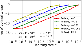
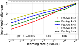
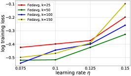
Figure 2: Optimality gap $\{f(\mathbf{w}_{\texttt{FedAvg}}^{*})-f^{*}\}$ or training loss $\{f(\mathbf{w}_{\texttt{FedAvg}}^{*})\}$ of (approximate) fixed-point solutions of FedAvg for different learning rates $\eta$ and local epochs $k$. Different colored lines are for different numbers of local epochs, and dashed lines for different product values $\eta(k-1)$. Left: least squares (closed-form solution); Middle: logistic regression ($6000$ communication rounds); Right: nonconvex CNN on the MNIST dataset ($200$ communication rounds).

3.2 FedProx as backward-backward splitting

The recent FedProx algorithm [2] replaces the gradient update in FedAvg with a proximal update:

$$\mathsf{w}_{t+1}=\mathsf{P}_{H}\mathsf{P}_{\mathsf{f}}^{\eta_{t}}\mathsf{w}_{t},$$ (12)

where as before we may use a minibatch to approximate $\mathsf{P}_{\mathsf{f}}^{\eta}$ or select a subset of users to approximate $\mathsf{P}_{H}$. Written in this way, it is clear that FedProx is an instantiation of the backward-backward splitting algorithm of [44, 45]. In fact, this algorithm traces back to the early works of e.g. [46, 47, 48], sometimes under the name of the Barycenter method. It was also rediscovered by [49, 50] in the ML community under a somewhat different motivation. [5] pointed out that FedProx does not solve the original problem (1). While technically correct, their conclusion did not take many other subtleties into account, which we explain next.

Following [51], we first note that, with a constant step size $\eta_{t}\equiv\eta$, FedProx is actually equivalent as FedAvg but applied to a “regularized” problem:

$$\min_{\mathsf{w}\in H}\leavevmode\nobreak\ \leavevmode\nobreak\ \tilde{\mathsf{f}}(\mathsf{w}),\leavevmode\nobreak\ \leavevmode\nobreak\ \mathrm{where}\ \leavevmode\nobreak\ \leavevmode\nobreak\ \tilde{\mathsf{f}}(\mathsf{w}):=\left\langle\mathbf{1},\mathsf{M}_{\mathbf{f}}^{\eta}(\mathsf{w})\right\rangle,\leavevmode\nobreak\ \mbox{ and }\leavevmode\nobreak\ \mathsf{M}_{\mathbf{f}}^{\eta}(\mathsf{w})=\big{(}\mathsf{M}_{f_{1}}^{\eta}(\mathbf{w}_{1}),\ldots,\mathsf{M}_{f_{m}}^{\eta}(\mathbf{w}_{m})\big{)}.$$ (13)

Interestingly, [15] proposed exactly (13) for the purpose of personalization, which we now realize is automatically achieved if we apply FedProx to the original formulation (1). Indeed, $\nabla\mathsf{M}_{\mathbf{f}}^{\eta}(\mathsf{w})=[\mathsf{w}-\mathsf{P}_{\mathbf{f}}^{\eta}(\mathsf{w})]/\eta$ hence $\mathsf{G}_{\tilde{f}}^{\eta}(\mathsf{w})=\mathsf{w}-\eta\nabla\tilde{\mathsf{f}}(\mathsf{w})=\mathsf{P}_{\mathbf{f}}^{\eta}(\mathsf{w})=\big{(}\mathsf{P}_{f_{1}}^{\eta}(\mathbf{w}_{1}),\ldots,\mathsf{P}_{f_{m}}^{\eta}(\mathbf{w}_{m})\big{)}$. This simple observation turns out to be crucial in understanding FedProx.

Indeed, a significant challenge in FL is user heterogeneity (a.k.a. non-iid distribution of data), where the individual user functions $f_{i}$ may be very different (due to distinct user-specific data). But, we note that as $\eta\to 0$, $\mathsf{M}_{f}^{\eta}\to f$ (pointwise or uniformly if $f$ is Lipschitz) while $\mathsf{M}_{f}^{\eta}\to\min f$ as $\eta\to\infty$. In other words, a larger $\eta$ in (13) “smoothens” heterogeneity in the sense that the functions $\mathsf{M}_{f_{i}}^{\eta}$ tend to have similar minimizers (while the minimum values may still differ). We are thus motivated to understand the convergence behaviour of FedProx, for small and large $\eta$, corresponding to the original problem (1) and the smoothened problem, respectively. In fact, we can even adjust $\eta$ dynamically. Below, for simplicity, we assume full gradient (i.e. large batch size) although extensions to stochastic gradient are possible.

Theorem 1.

Assuming each user participates indefinitely, the step size $\eta_{t}$ is bounded from below (i.e. $\liminf_{t}\eta_{t}>0$), the user functions $\{f_{i}\}$ are convex, and homogeneous in the sense that they have a common minimizer, i.e. $\mathsf{F}:=\bigcap_{i}\operatorname*{argmin}_{\mathbf{w}_{i}}\leavevmode\nobreak\ f_{i}(\mathbf{w}_{i})\neq\emptyset$, then the iterates of FedProx converge to a point in $\mathsf{F}$, which is a correct solution of (1).

The homogeneity assumption might seem strong since it challenges the necessity of FL in the first place. However, we point out that (a) as a simplified limiting case it does provide insight on when user functions have close minimizers (i.e. homogeneous); (b) by using a large step size $\eta$ FedProx effectively homogenizes the users and its convergence thus follows; (c) modern deep architectures are typically over-parameterized so that achieving null training loss on each user is not uncommon. However, FL is still relevant even in this case since it selects a model that works for every user and hence provides some regularizing effect; (d) even when the homogeneity assumption fails, $\mathsf{P}_{\mathsf{f}}^{\eta_{t}}$ still converges to a point that is in some sense closest to $H$ [51].

The next result removes the homogeneity assumption by simply letting step size $\eta_{t}$ diminish:

Theorem 2 ([44, 45]).

Assuming each user participates in every round, the step size $\eta_{t}$ satisfies $\sum_{t}\eta_{t}=\infty$ and $\sum_{t}\eta_{t}^{2}<\infty$, and the functions $\{f_{i}\}$ are convex, then the averaged iterates $\bar{\mathsf{w}}_{t}:=\tfrac{\sum_{s=1}^{t}\eta_{s}\mathsf{w}_{s}}{\sum_{s=1}^{t}\eta_{s}}$ of FedProx converge to a correct solution of the original problem (1).

In Appendix C, we give examples to show the tightness of the step size condition in Theorem 2. We emphasize that $\bar{\mathsf{w}}_{t}$ converges to a solution of the original problem (1), not the regularized problem (13). The subtlety is that we must let the step size $\eta_{t}$ approach 0 reasonably slowly, a possibility that was not discussed in [5] where they always fixed the step size $\eta_{t}$ to a constant $\eta$. Theorem 2 also makes intuitive sense, as $\eta_{t}\to 0$ slowly, we are effectively tracking the solution of the regularized problem (13) which itself tends to the original problem (1): recall that $\mathsf{M}_{f}^{\eta}\to f$ as $\eta\to 0$.

Even the ergodic averaging step in Theorem 2 can be omitted in some cases:

Theorem 3 ([45]).

Under the same assumptions as in Theorem 2, if $\mathbf{f}$ is strongly convex or the solution set of (1) has nonempty interior, then the vanilla iterates $\mathsf{w}_{t}$ of FedProx also converge.

We remark that convergence is in fact linear for the second case. Nevertheless, the above two conditions are perhaps not easy to satisfy or verify in most applications. Thus, in practice, we recommend the ergodic averaging in Theorem 2 since it does not create additional overhead (if implemented incrementally) and in our experiments it does not slow down the algorithm noticeably.

There is in fact a quantitative relationship between the original problem (1) and the regularized problem (13), even in the absence of convexity:

Theorem 4 ([50]).

Suppose each $f_{i}$ is $M_{i}$-Lipschitz continuous (and possibly nonconvex), then

$$\textstyle\forall\mathsf{w},\leavevmode\nobreak\ \leavevmode\nobreak\ \leavevmode\nobreak\ f(\mathsf{w})-\tilde{f}(\mathsf{w})\leq\sum_{i}\lambda_{i}\tfrac{\eta M_{i}^{2}}{2}.$$ (14)

Thus, for a small step size $\eta$, FedProx, aiming to minimize the regularized function $\tilde{\mathsf{f}}$ is not quantitatively different from FedAvg that aims at minimizing $\mathsf{f}$. This again reveals the fundamental importance of step size in FL. We remark that, following the ideas in [50], we may remove the need of ergodic averaging for FedProx if the functions $f_{i}$ are “definable” (which most, if not all, functions used in practice are). We omit the technical complication here since the potential gain does not appear to be practically significant.

In Figure 3, we show the effect of step size $\eta$ on the convergence of FedProx, and compare the results with that of FedAvg on both convex and nonconvex models. We run FedProx with both fixed and diminishing step sizes. In the experiments with diminishing step sizes, we have set the initial value of $\eta$ (i.e. $\eta_{0}$) to larger values - compared to the constant $\eta$ values - to ensure that $\eta$ does not get very small after the first few rounds. From the convex experiments (Fig 3, left and middle), one can see that FedProx with a fixed learning rate converges fast (in a few hundred rounds) to a suboptimal solution. In contrast, FedProx with diminishing $\eta$ converges slower, but to better quality solutions. It is interesting to note that only when the conditions of Theorem 2 are satisfied (i.e. $\eta$ diminishes neither too fast nor too slow), FedProx converges to a correct solution of the original problem (1), e.g. see the results for $\eta_{t}\propto 1/t$ which satisfies both conditions in Theorem 2. Surprisingly, for the nonconvex setting (Figure 3, right), the best results are achieved with larger learning rates. A similar observation about FedAvg in nonconvex settings was reported in [1, Fig. 5 & 6]. Moreover, from the results on both convex and nonconvex models, one can see that ergodic averaging does not affect the convergence rate of FedProx noticeably.

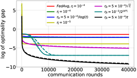
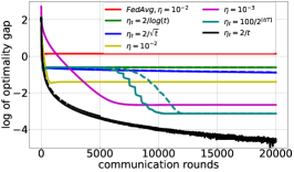
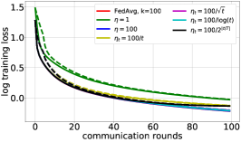
Figure 3: Effect of step size $\eta$ and averaging on FedProx. Left: least squares; Middle: logistic regression; Right: CNN on MNIST. The dashed and solid lines with the same color show the results obtained with and without the ergodic averaging step in Theorem 2, respectively. For exponentially decaying $\eta_{t}$, we use period $T$ equal to $500$ for both least squares and logistic regression experiments, and $10$ for CNN experiment.

3.3 FedSplit as Peaceman-Rachford splitting

[5] introduced the FedSplit algorithm recently:

$$\mathsf{w}_{t+1}=\mathsf{R}_{H}\mathsf{R}_{\mathsf{f}}^{\eta_{t}}\mathsf{w}_{t},$$ (15)

which is essentially an instantiation of the Peaceman-Rachford splitting algorithm [35, 36]. As shown by [36], FedSplit converges to a correct solution of (1) if $\mathbf{f}$ is strictly convex, and the convergence rate is linear if $\mathbf{f}$ is strongly convex and smooth (and $\eta$ is small). [5] also studied the convergence behaviour of FedSplit when the reflector $\mathsf{R}_{\mathsf{f}}^{\eta}$ is computed approximately. However, we note that convergence behaviour of FedSplit is not known or widely studied for nonconvex problems. In particular, we have the following surprising result:

Theorem 5.

If the reflector $\mathsf{R}_{f}^{\eta}$ is a (strict) contraction, then $f$ must be strongly convex.

The converse is true if $f$ is also smooth and $\eta$ is small [36, 53]. Therefore, for non-strongly convex or nonconvex problems, we cannot expect FedSplit to converge linearly (if it converges at all).

3.4 FedPi as Douglas-Rachford splitting

A popular alternative to the Peaceman-Rachford splitting is the Douglas-Rachford splitting [37, 36], which, to our best knowledge, has not been applied to the FL setting. The resulting update, which we call FedPi, can be written succinctly as:

$$\mathsf{w}_{t+1}=\tfrac{\mathsf{w}_{t}+\mathsf{R}_{H}\mathsf{R}_{\mathsf{f}}^{\eta_{t}}\mathsf{w}_{t}}{2},$$ (16)

i.e. we simply average the current iterate and that of FedSplit evenly. Strictly speaking, the above algorithm is a special case of the Douglas-Rachford splitting and was rediscovered by [54] under the name of partial inverse (hence our name FedPi). The moderate averaging step in (16) makes FedPi much more stable:

Theorem 6 ([54, 36]).

Assuming each user participates in every round, the step size $\eta_{t}\equiv\eta$ is constant, and the functions $\{f_{i}\}$ are convex, then the vanilla iterates $\mathsf{w}_{t}$ of FedPi converge to a correct solution of the original problem (1).

Compared to FedSplit, FedPi imposes less stringent condition on $f_{i}$. However, when $f_{i}$ is indeed strongly convex and smooth, as already noted by [36], FedPi will be slower than FedSplit by a factor close to $\sqrt{2}$ (assuming the constant step size is set appropriately for both). More importantly, it may be easier to analyze FedPi on nonconvex functions, as recently demonstrated in [55, 56].

Interestingly, FedPi also has close ties to FedProx. Indeed, this is best seen by expanding the concise formula in (16) and introducing a “dual variable” $\mathsf{u}$ on the server side:

$$\mathsf{z}_{t+1} \leftarrow\mathsf{P}_{\mathsf{f}}^{\eta}(\mathsf{w}_{t}+\mathsf{u}_{t})$$ (17)

$$\mathsf{w}_{t+1} \leftarrow\mathsf{P}_{H}(\mathsf{z}_{t+1}{\color[rgb]{.5,.5,.5}-\mathsf{u}_{t}})$$ (18)

$$\mathsf{u}_{t+1} \leftarrow\mathsf{u}_{t}+\mathsf{w}_{t+1}-\mathsf{z}_{t+1}.$$ (19)

From the last two updates (18) and (19) it is clear that $\mathsf{u}_{t+1}$ is always in $H^{\perp}$. Thus, after performing a change of variable $\mathsf{v}_{t}:=\mathsf{w}_{t}+\mathsf{u}_{t}$ and exploiting the linearity of $\mathsf{P}_{H}$, we obtain exactly FedPi:

$$\mathsf{v}_{t+1}=\mathsf{u}_{t}+2\mathsf{w}_{t+1}-\mathsf{z}_{t+1}=\mathsf{v}_{t}-\mathsf{P}_{H}\mathsf{v}_{t}+2\mathsf{P}_{H}\mathsf{P}_{\mathsf{f}}^{\eta}\mathsf{v}_{t}-\mathsf{P}_{\mathsf{f}}^{\eta}\mathsf{v}_{t}=\tfrac{\mathsf{v}_{t}+\mathsf{R}_{H}\mathsf{R}_{\mathsf{f}}^{\eta}\mathsf{v}_{t}}{2}.$$ (20)

Comparing (12) and (17)-(18) it is clear that FedProx corresponds to fixing the dual variable $\mathsf{u}$ to the constant $\mathbf{0}$ in FedPi. We remark that step (17) is done at the users’ side while steps (18) and (19) are implemented at the server side. There is no communication overhead either, as the server need only communicate the sum $\mathsf{w}_{t}+\mathsf{u}_{t}$ to the respective users while the users need only communicate their $\mathbf{z}_{t,i}$ to the server. The dual variable $\mathsf{u}$ is kept entirely at the server’s expense.

Let us point out another subtle difference that may prove useful in FL: FedAvg and FedProx are inherently “synchronous” algorithms, in the sense that all participating users start from a common, averaged model at the beginning of each communication round. In contrast, the local models $\mathsf{z}_{t}$ in FedPi may be different from each other, where we “correct” the common, average model $\mathsf{w}_{t}$ with user-specific dual variables $\mathsf{u}_{t}$. This opens the possibility to personalization by designating the dual variable $\mathsf{u}$ in user-specific ways.

Lastly, we remark that in FedProx we need the step size $\eta_{t}$ to diminish in order to converge to a solution of the original problem (1) whereas FedPi achieves the same with a constant step size $\eta$, although at the cost of doubling the memory cost at the server side.

3.5 FedRP as Reflection-Projection splitting

Examining the updates in (9), (12) and (15), we are naturally led to the following further variants (that have not been tried in FL to the best of our knowledge):

$$\mathsf{w}_{t+1} =\mathsf{R}_{H}\mathsf{G}_{\mathsf{f}}^{\eta_{t}}\mathsf{w}_{t}$$ (21)

$$\mathsf{w}_{t+1} =\mathsf{R}_{H}\mathsf{P}_{\mathsf{f}}^{\eta_{t}}\mathsf{w}_{t}$$ (22)

$$\mbox{{FedRP}}:\qquad\mathsf{w}_{t+1} =\mathsf{P}_{H}\mathsf{R}_{\mathsf{f}}^{\eta_{t}}\mathsf{w}_{t}.$$ (23)

Interestingly, the last variant in (23), which we call FedRP, has been studied by [39] under the assumption that $\mathsf{f}=\iota_{\mathsf{K}}$ is an indicator function of an obtuse convex cone $\mathsf{K}$. We prove the following result for FedRP:

Theorem 7.

Let each user participate in every round and the functions $\{f_{i}\}$ be convex. If the step size $\eta_{t}\equiv\eta$ is constant, then any fixed point of FedRP is a solution of the regularized problem (13). If the reflector $\mathsf{R}_{\mathsf{f}}^{\eta}$ is idempotent (i.e. $\mathsf{R}_{\mathsf{f}}^{\eta}\mathsf{R}_{\mathsf{f}}^{\eta}=\mathsf{R}_{\mathsf{f}}^{\eta}$) and the users are homogeneous, then the vanilla iterates $\mathsf{w}_{t}$ of FedRP converge.

It follows easily from a result in [39] that a convex cone is obtuse iff its reflector is idempotent, and hence Theorem 7 strictly extends their result. We remark that Theorem 7 does not apply to the variants (21) and (22) since the reflector $\mathsf{R}_{H}$ is not idempotent (recall $H$ is defined in (4)). Of course, we can prove (linear) convergence of both variants (21) and (22) if $\mathsf{f}$ is strongly convex. We omit the formal statement and proof since strong convexity does not appear to be easily satisfiable in practice.

In Figure 4, we compare the performance of different splitting algorithms and how they respond to different degrees of user heterogeneity. We use least squares and a CNN model on MNIST for the convex and noconvex experiments, respectively. The details of the experimental setup are described in Section A.1. For the convex setting, as expected, FedSplit, FedPi, and FedAvg with $k=1$ achieve the smallest optimality gaps. The performance of all the algorithms deteriorates as users’ data become more heterogeneous (see Section A.1). For the nonconvex setting, the best results can be achieved by FedRP and FedAvg with a big $k$. It is noteworthy that in the nonconvex setting, the performance of FedAvg with $k=1$ is significantly worse than that with $k=100$.

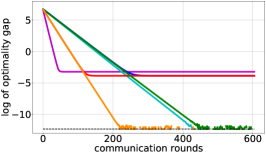
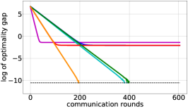
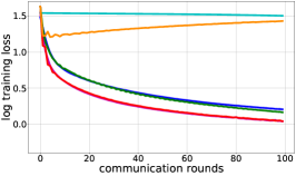
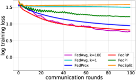
Figure 4: The effect of data heterogeneity on the performance of different splitting methods. The top row shows the results for the least squares, and the bottom row shows the results for nonconvex CNN model. Top-Left: small data heterogeneity with $H\approx 119\times 10^{3}$; Top-Middle: moderately data heterogeneity with $H\approx 7.61\times 10^{6}$; Top-Right: large data heterogeneity with $H\approx 190.3\times 10^{6}$. Bottom-Left: i.i.d. data distribution; Bottom-Middle: non-i.i.d. data distribution with maximum $6$ classes per user; Bottom-Right: non-i.i.d. data distribution with maximum $2$ classes per user.

4 Unification, implementation and acceleration

The operator splitting view of FL not only allows us to compare and understand the many existing FL algorithms but also opens the door for unifying and accelerating them. In this section we first introduce a grand scheme that unifies all aforementioned FL algorithms. Then, we provide two implementation variants that can accommodate different hardware and network constraints. Lastly, we explain how to adapt Anderson acceleration [40] to the unified FL algorithm, with almost no computation or communication overhead.

Unification.

We introduce the following grand scheme:

$$\mathsf{z}_{t+1} =(1-\alpha_{t})\mathsf{u}_{t}+\alpha_{t}\mathsf{P}_{\mathsf{f}}^{\eta_{t}}(\mathsf{u}_{t})$$ (24)

$$\mathsf{w}_{t+1} =(1-\beta_{t})\mathsf{z}_{t+1}+\beta_{t}\mathsf{P}_{H}(\mathsf{z}_{t+1})$$ (25)

$$\mathsf{u}_{t+1} =(1-\gamma_{t})\mathsf{u}_{t}+\gamma_{t}\mathsf{w}_{t+1}.$$ (26)

Table 1 confirms that the FL algorithms discussed in Section 3 are all special cases of this unifying scheme, which not only provides new (adaptive) variants but also clearly reveals the similarities and differences between seemingly different algorithms. It may thus be possible to transfer progress on one algorithm to the others and vice versa. We studied the effect of $\alpha$, $\beta$ and $\gamma$ and found that $\gamma$ mostly affects the convergence speed: the closer $\gamma$ is to 1, the faster the convergence is, while $\alpha$ and $\beta$ mostly determine the final optimality gap: the closer they are both to 2 (as in FedSplit and FedPi), the considerably smaller the final optimality gap is. However, setting only one of them close to 2 only has a minor effect on optimality gap or convergence speed.

Implementation.

Interestingly, we also have two implementation possibilities:

• decentralized: In this variant, all updates in (24)-(26) are computed and stored locally at each user while the server only acts as a bridge for synchronization: it receives $\mathbf{z}_{t+1,i}$ from the $i$-th user and returns the (same) averaged model $\mathsf{P}_{H}(\mathsf{z}_{t+1})$ to all users. In a network where users communicate directly with each other, we may then dispense the server and become fully decentralized.

• centralized: In this variant, the $i$-th user only stores $\mathbf{u}_{t,i}$ and is responsible for computing and communicating $\mathsf{P}_{f_{i}}^{\eta_{t}}(\mathbf{u}_{t,i})$ to the server. In return, the server performs the rest of (24)-(26) and then sends (different) $\mathbf{u}_{t+1,i}$ back to the $i$-th user.

The two variants are of course mathematically equivalent in their basic form. However, as we see below, they lead to different acceleration techniques and we may prefer one over the other depending on the hardware and network constraints.

Table 1: A unifying framework (24)-(26) for FL. Note that (a) FedAvg replaces the proximal update $\mathsf{P}_{\mathsf{f}}^{\eta}$ with a gradient update $\mathsf{G}_{\mathsf{f},k}^{\eta}$; (b) ? indicates properties that remain to be studied; (c) “sampling” refers to selecting a subset of users while “stochastic” refers to updating with stochastic gradient.

Algorithm	$\alpha$	$\beta$	$\gamma$	$\eta_{t}\!\equiv\!\eta$	$\eta_{t}\!\to\!0,\sum_{t}\eta_{t}\!=\!\infty$	nonconvex	sampling	stochastic
FedAvg	1	1	1	eq. 1	eq. 1	✓	✓	✓
FedProx	1	1	1	eq. 13	eq. 1	✓	✓	✓
FedSplit	2	2	1	eq. 1	–	?	?	?
FedPi	2	2	$\tfrac{1}{2}$	eq. 1	–	✓	?	?
FedRP	2	1	1	eq. 13	eq. 1	?	?	?

Acceleration.

Let us abstract the grand scheme (24)-(26) as the map $\mathsf{u}_{t+1}=\mathsf{T}\mathsf{u}_{t}$, where $\mathsf{T}$ is nonexpansive if $\mathsf{f}$ is convex and $\alpha_{t},\beta_{t}\in[0,2],\gamma_{t}\in[0,1]$. Following [41], we may then apply the Anderson type-II acceleration to furthur improve convergence. Let $U=[\mathsf{u}_{t-\tau},\ldots,\mathsf{u}_{t}]$ be given along with $T=[\mathsf{T}\mathsf{u}_{t-\tau},\ldots,\mathsf{T}\mathsf{u}_{t}]$. We solve the following simple least-squares problem:

$$\bm{\pi}^{*}=\operatorname*{argmin}_{\bm{\pi}^{\top}\mathbf{1}=1}\leavevmode\nobreak\ \{\|(U-T)\bm{\pi}\|_{2}^{2}\}=\tfrac{G^{\dagger}\mathbf{1}}{\mathbf{1}^{\top}G^{\dagger}\mathbf{1}},\leavevmode\nobreak\ \leavevmode\nobreak\ \mathrm{where}\ \leavevmode\nobreak\ \leavevmode\nobreak\ G=(U-T)^{\top}(U-T).$$ (27)

(For simplicity we do not require $\bm{\pi}$ to be nonnegative.) Then, we update $\mathsf{u}_{t+1}=T\bm{\pi}^{*}$. Clearly, when $\tau=0$, (trivially) $\pi^{*}=1$ and we reduce to $\mathsf{u}_{t+1}=\mathsf{T}\mathsf{u}_{t}$. With a larger memory size $\tau$, we may significantly improve convergence. Importantly, all heavy lifting (computation and storage) is done at the server side and we do not increase communication at all. We note that the same acceleration can also be applied on each user for computing $\mathsf{P}_{\mathsf{f}}^{\eta_{t}}$, if the users can afford the memory cost.

We have already seen how different variants (e.g. FedAvg, FedProx, FedSplit, FedPi, FedRP) compare to each other in §3. We performed further experiments to illustrate their behaviour under Anderson acceleration. (See Appendix A for details on our experimental setup.) As can be observed in Figure 5, Anderson acceleration helps FL algorithms converge considerably faster, all without incurring any overhead. For the convex models (least squares and logistic regression), our implementation of Anderson-acceleration speeds up all of the algorithms, especially FedAvg, FedProx and FedRP. However, for the nonconvex CNN model, it is beneficial only for FedAvg, FedProx and FedPi, while applying it to FedRP and FedSplit makes them unstable. It is noteworthy that we already know FedProx and FedPi are more stable than FedRP and FedSplit, respectively, and hence it makes intuitive sense that acceleration improves the two more stable algorithms. Another important point we wish to point out is that our acceleration method does not affect the quality of the algorithms’ final solutions, but rather it just accelerates their convergence.

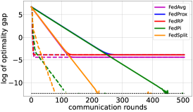
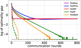
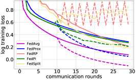
Figure 5: Effect of Anderson acceleration. Left: least squares with $\tau=2$; Middle: logistic regression $\tau=2$; Right: nonconvex CNN with $\tau=10$. Dashed lines are the accelerated results.

5 Conclusions

We have connected FL with the established theory of operator splitting, revealed new insights on existing algorithms and suggested new algorithmic variants and analysis. Our unified view makes it easy to understand, compare, implement and accelerate different FL algorithms in a streamlined and standardized fashion. Our experiments demonstrate some interesting differences in the convex and nonconvex settings, and in the early and late communication rounds. In the future we plan to study the effect of stochasticity and extend our analysis to nonconvex functions. While our initial experiments confirmed the potential of Anderson-acceleration for FL, further work is required to formalize its effect in theory (such as [58]) and to understand its relation with other momentum methods in FL.

Appendix A Experimental Setup

In this section we provide more experimental details that are deferred from the main paper.

A.1 Experimental setup: Least Squares and Logistic Regression

For simulating an instance of the aforementioned least squares and logistic regression problems, we follow the experimental setup of [5].

Least squares regression:

We consider a set of $m$ users with local loss functions $f_{i}(\mathbf{w}):=\frac{1}{2}\|A_{i}\mathbf{w}-\mathbf{b}_{i}\|_{2}^{2}$, and the main goal is to solve the following minimization problem:

$$\min_{\mathbf{w}\in\mathds{R}^{d}}\leavevmode\nobreak\ F(\mathbf{w}):=\sum_{i=1}^{m}f_{i}(\mathbf{w})=\frac{1}{2}\sum_{i=1}^{m}\|A_{i}\mathbf{w}-\mathbf{b}_{i}\|_{2}^{2},$$

where $\mathbf{w}\in\mathds{R}^{d}$ is the optimization variable. For each user $i$, the response vector $\mathbf{b}_{i}\in\mathds{R}^{n_{i}}$ is related to the design matrix $A_{i}\in\mathds{R}^{n_{i}\times d}$ via the linear model

$$\centering\mathbf{b}_{i}=A_{i}\mathbf{w}_{\star}+\bm{\epsilon}_{i},\@add@centering$$

where $\bm{\epsilon}_{i}\sim N(0,\sigma^{2}I_{n_{i}})$ for some $\sigma>0$ is the noise vector. The design matrix $A_{i}\in\mathds{R}^{n_{i}\times d}$ is generated by sampling its elements from a standard normal, $A_{i}^{k,l}\sim N(0,1)$. We instantiated the problem with the following set of parameters:

$$\centering m=25,\leavevmode\nobreak\ \leavevmode\nobreak\ d=100,\leavevmode\nobreak\ \leavevmode\nobreak\ n_{i}=5000,\leavevmode\nobreak\ \leavevmode\nobreak\ \sigma^{2}=0.25.\@add@centering$$

Binary logistic regression:

There are $m$ users and the design matrices $A_{i}\in\mathds{R}^{n_{i}\times d}$ for $i=1,\ldots,m$ are generated as described before. Each user $i$ has a label vector $\mathbf{b}_{i}\in\{-1,1\}^{n_{i}}$. The conditional probability of observing $\mathbf{b}_{ij}=1$ (the $j$-th label in $\mathbf{b}_{i}$) is

$$\centering\mathbf{P}\{\mathbf{b}_{ij}=1\}=\frac{e^{\mathbf{a}_{ij}^{\top}\mathbf{w}_{0}}}{1+e^{\mathbf{a}_{ij}^{\top}\mathbf{w}_{0}}},\leavevmode\nobreak\ \leavevmode\nobreak\ \leavevmode\nobreak\ j=1,\ldots,n_{i},\@add@centering$$

where $\mathbf{a}_{ij}$ is the $j$-th row of $A_{i}$. Also, $\mathbf{w}_{0}\in\mathds{R}^{d}$ is fixed and sampled from $N(0,1)$. Having generated the design matrices $A_{i}$ and sampled the labels $\mathbf{b}_{i}$ for all users, we find the maximum likelihood estimate of $\mathbf{w}_{0}$ by solving the following convex program, which has a solution $\mathbf{w}_{*}$:

$$\min_{\mathbf{w}\in\mathds{R}^{d}}\leavevmode\nobreak\ F(\mathbf{w}):=\sum_{i=1}^{m}f_{i}(\mathbf{w})=\sum_{i=1}^{m}\sum_{j=1}^{n_{i}}\log(1+e^{-b_{ij}\mathbf{a}_{ij}^{\top}\mathbf{w}})+\frac{\|\mathbf{w}\|_{2}^{2}}{2mn_{i}}.$$

Following [5], we set

$$\centering m=10,\leavevmode\nobreak\ \leavevmode\nobreak\ d=100,\leavevmode\nobreak\ \leavevmode\nobreak\ n_{i}=1000.\@add@centering$$

Data heterogeneity measure:

We adopt the data heterogeneity measure of [11], and quantify the amount of heterogeneity in users’ data for the least squares and logistic regression problems by

$$H:=\frac{1}{m}\sum_{i=1}^{m}\parallel\nabla f_{i}(\mathbf{w}_{*})\parallel_{2}^{2},$$

where $\mathbf{w}_{*}$ is a minimizer of the original problem (1). When users’ data is homogeneous, all the local functions $f_{i}$ have the same minimizer of $\mathbf{w}_{*}$ and $H=0$. In general, the more heterogeneous the users’ data is, the larger $H$ becomes.

Other parameters:

Throughout the experiments, we use local learning rate $\eta=10^{-5}$ for least squares, and $\eta=10^{-2}$ for logistic regression, and run FedAvg with $k=5$ for both least squares and logistic regression, unless otherwise specified. In Figure 5, FedAvg is run with $k=2$.

A.2 Experimental setup: MNIST datasets

We consider a distributed setting with $20$ users. In order to create a non-i.i.d. dataset, we follow a similar procedure as in [1]: first we split the data from each class into several shards. Then, each user is randomly assigned a number of shards of data. For example, in Figure 4 to guarantees that no user receives data from more than $6$ classes, we split each class of MNIST into $12$ shards (i.e., a total of $120$ shards for the whole dataset), and each user is randomly assigned $6$ shards of data. By considering $20$ users, this procedure guarantees that no user receives data from more than $6$ classes and the data distribution of each user is different from each other. The local datasets are balanced–all users have the same amount of training samples. The local data is split into train, validation, and test sets with percentage of $80$%, $10$%, and $10$%, respectively. In this way, each user has $2400$ data points for training, $300$ for test, and $300$ for validation. We use a simple 2-layer CNN model with ReLU activation, the detail of which can be found in Table 2. To update the local models at each user using its local data, unless otherwise is stated, we apply gradient descent with $\eta=0.01$ for FedAvg, and gradient descent with $k=100$ and $\eta=0.01$ for proximal update in the splitting algorithms.

Table 2: MNIST model

Layer	Output Shape	$\#$ of Trainable Parameters	Activation	Hyper-parameters
Input	$(1,28,28)$	$0$
Conv2d	$(10,24,24)$	$260$	ReLU	kernel size =$5$; strides=$(1,1)$
MaxPool2d	$(10,12,12)$	$0$		pool size=$(2,2)$
Conv2d	$(20,8,8)$	$5,\!020$	ReLU	kernel size =$5$; strides=$(1,1)$
MaxPool2d	$(20,4,4)$	$0$		pool size=$(2,2)$
Flatten	$320$	$0$
Dense	$20$	$6,\!420$	ReLU
Dense	$10$	$210$	softmax
Total		$11,\!910$

A.3 Experimental setup: CIFAR-10 dataset

We consider a distributed setting with $10$ users, and use a sub-sampled CIFAR-10 dataset, which is $20\%$ of the training set. In order to create a non-i.i.d. dataset, we follow a similar procedure as in [1]: first we sort all data points according to their classes. Then, they are split into $100$ shards, and each user is randomly assigned $10$ shards of data. The local data is split into train, validation, and test sets with percentage of $80$%, $10$%, and $10$%, respectively. In this way, each user has $800$ data points for training, $100$ for test, and $100$ for validation. We use a 2-layer CNN model on the dataset, , the detail of which can be found in Table 3. To update the local models at each user using its local data, we apply stochastic gradient descent (SGD) with local batch size $B=20$ and local learning rate $\eta=0.1$. All users participate in each communication round.

Table 3: CIFAR-10 model

Layer	Output Shape	$\#$ of Trainable Params	Activation	Hyper-parameters
Input	$(3,32,32)$	$0$
Conv2d	$(64,28,28)$	$4,\!864$	ReLU	kernel =$5$; strides=$(1,1)$
MaxPool2d	$(64,14,14)$	$0$		pool size=$(2,2)$
LocalResponseNorm	$(64,14,14)$	$0$		size=$2$
Conv2d	$(64,10,10)$	$102,\!464$	ReLU	kernel =$5$; strides=$(1,1)$
LocalResponseNorm	$(64,10,10)$	$0$		size=$2$
MaxPool2d	$(64,5,5)$	$0$		pool size=$(2,2)$
Flatten	$1,\!600$	$0$
Dense	$384$	$614,\!784$	ReLU
Dense	$192$	$73,\!920$	ReLU
Dense	$10$	$1,\!930$	softmax
Total		$797,\!962$

Appendix B Full experiments

In this section we provide more experimental results that are deferred from the main paper.

B.1 FedRP experiments to supplement Figure 2

In Figure 6, we show the effect of step size $\eta$ on the convergence of FedRP on least squares and logistic regression. We run FedRP with both fixed and diminishing step sizes. In the experiments with diminishing step sizes, we set the initial value of $\eta$ (i.e. $\eta_{0}$) to larger values–compared to the constant $\eta$ values–to ensure that $\eta$ does not get very small after the first few rounds. From the figure, one can see that FedRP with a fixed learning rate converges faster in early stage but to a sub-optimal solution. In contrast, FedRP with diminishing $\eta$ converges slower early, but to better final solutions. It is interesting to note that the convergence behaviour of FedRP is similar to that of FedProx and when the conditions of Theorem 2 are satisfied, FedRP converges to a correct solution of the original problem (1), e.g. see the results for $\eta_{t}\propto 1/t$ which satisfies both conditions in Theorem 2. Moreover, one can see that ergodic averaging hardly affects the convergence of FedRP in the following results.

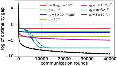
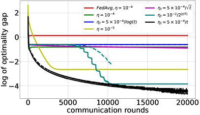
Figure 6: Effect of step size $\eta$ and averaging on FedRP. Left: least squares; Right: logistic regression. The dashed and solid lines with the same color show the results obtained with and without the ergodic averaging step in Theorem 2, respectively. For exponentially decaying $\eta_{t}$, we use period $T$ equal to $500$ for both least squares and logistic regression.

B.2 Effect of changing $k$ or $\eta$ for FedAvg

In Figure 7, we observe a trade-off between faster (early) convergence and better final solution when varying local epochs $k$ or learning rate $\eta$, in least squares and logistic regression experiments. When $\eta$ is fixed, larger local epochs $k$ leads to faster convergence (in terms of communication rounds) during the early stages, at the cost of a worse final solution. When local epochs $k$ is fixed, same trade-off holds true for increasing $\eta$.

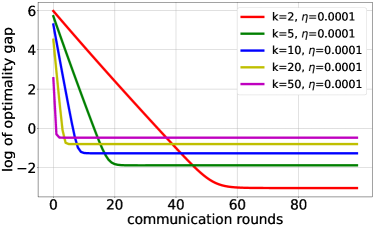
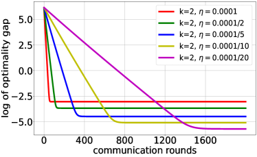
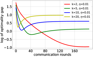
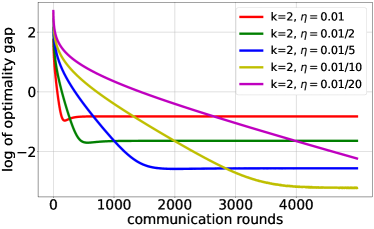
Figure 7: Convergence of FedAvg changing $k$ or $\eta$. Top: least squares; Bottom: logistic regression.

In Figure 8, contrary to what we observe in the previous convex experiments where fixed learning rate with less local epochs leads to a better final solution at the expense of slower convergence, we do not see similar trade-offs in this nonconvex setting, (at least) given the computation we can afford. This is probably because the solution we get is still in early stage due to the combined complexity of CNN and CIFAR-10 dataset, compared to the relatively simple least squares and logistic regression we had before.

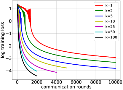
Figure 8: Running FedAvg on CIFAR-10 with different number of local epochs $k$. The number of users is $10$, local learning rate $\eta=0.1$. Data points are sampled and distributed to users non-uniformly.

B.3 Effect of user sampling

The grand scheme introduced in (24)-(26) assumes that all users participate in each communication round–full user participation; however, this might not be always the case. So, we modify the grand scheme to investigate the effect of user participation. The modified version, which is based on the centralized implementation of FL algorithms (explained in section 4), is given in Algorithm 1. The simulation results for least squares and logistic regression are shown in Figure 9. From the results it can be observed that, with partial user participation, none of the aforementioned algorithms converge to the correct solution, especially FedAvg with $k=1$. Also, FedSplit becomes unstable when user participation is low ($p=0.5$), while other algorithms e.g. FedPi remain stable.

Input: $p$ (user participation probability), $\alpha_{t},\beta_{t},\gamma_{t},\eta_{t}$

Output: $\bar{\mathsf{w}}$ (final global model)

1

2initialize $\mathsf{u}_{0}$ and $\mathsf{z}_{0}$ for all users

3Server (p):

4       for each round $t=1,2,\ldots$ do

5             $S_{t}\leftarrow$ sample the set of present users, where each user participates with probability $p$

6            for each client $i$ in parallel do

7                   if $i\in S_{t}$ then

8                         ClientUpdate($\mathsf{u}_{i,t}$, $i$)

9                  else

10                         $\mathsf{z}_{i,t+1}\leftarrow\mathsf{z}_{i,t}$

             $\bar{\mathsf{w}}\leftarrow\mathsf{P}_{H}(\mathsf{z}_{t+1})$

              // over $\mathsf{z}_{t+1}$ of present clients

11            

12             $\mathsf{w}_{t+1}=(1-\beta_{t})\mathsf{z}_{t+1}+\beta_{t}\bar{\mathsf{w}}$

13            $\mathsf{u}_{t+1}=(1-\gamma_{t})\mathsf{u}_{t}+\gamma_{t}\mathsf{w}_{t+1}$

14ClientUpdate ($\mathsf{u}_{i,t}$, $i$):

       compute $\mathsf{P}_{f_{i}}^{\eta_{t}}(\mathsf{u}_{i,t})$

        // using standard gradient descent

15      

16      $\mathsf{z}_{i,t+1}\leftarrow(1-\alpha_{t})\mathsf{u}_{i,t}+\alpha_{t}\mathsf{P}_{f_{i}}^{\eta_{t}}(\mathsf{u}_{i,t})$

Algorithm 1 Federated learning with user sampling.

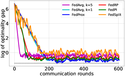
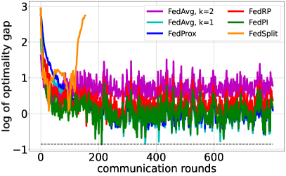
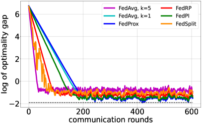
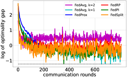
Figure 9: Effect of user sampling. $p$ denotes the probability that a user participates in a communication round. Top-Left: least squares with $p=0.5$; Top-Right: logistic regression with $p=0.5$; Bottom-Left: least squares with $p=0.7$; Bottom-Right: logistic regression with $p=0.7$.

B.4 Effect of using mini-batch gradient descent locally

Figure 10 shows the results when each user uses mini-batch gradient descent to update its model for different splitting algorithms. As in the grand scheme (24)-(26), we assume full user participation. Algorithm 2 summarizes the implementation details. As can be observed in the convex setting experiments, with mini-batch gradient descent used locally, none of the aforementioned algorithms converge to the correct solution. Furthermore, convergence speed of the algorithms decreases compared to when users use standard gradient descent. Also, FedAvg, even with $k=1$, does not outperform the other splitting algorithms, and FedSplit and FedPi converge to better solutions. On the other hand, in the nonconvex setting, FedAvg with $k=100$ achieves better solutions compared to the other algorithms.

1

Input: $B$ (local minibatch size), $\alpha_{t},\beta_{t},\gamma_{t},\eta_{t}$

Output: $\bar{\mathsf{w}}$ (final global model)

2

3initialize $\mathsf{u}_{0}$ for each user $i$

4Server :

5       for each round $t=1,2,\ldots$ do

6            

7            for each client $i$ in parallel do

8                   ClientUpdate($\mathsf{u}_{i,t},i$)

9             $\bar{\mathsf{w}}\leftarrow\mathsf{P}_{H}(\mathsf{z}_{t+1})$

10             $\mathsf{w}_{t+1}=(1-\beta_{t})\mathsf{z}_{t+1}+\beta_{t}\bar{\mathsf{w}}$

11            $\mathsf{u}_{t+1}=(1-\gamma_{t})\mathsf{u}_{t}+\gamma_{t}\mathsf{w}_{t+1}$

12ClientUpdate ($\mathsf{u}_{i,t},i$):

       compute $\mathsf{P}_{f_{i}}^{\eta_{t}}(\mathsf{u}_{i,t})$

        // using minibatch gradient descent with batch size $B$

13      

14      $\mathsf{z}_{i,t+1}\leftarrow(1-\alpha_{t})\mathsf{u}_{i,t}+\alpha_{t}\mathsf{P}_{f_{i}}^{\eta_{t}}(\mathsf{u}_{i,t})$

Algorithm 2 Mini-batch Gradient Descent for local computations.

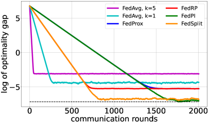
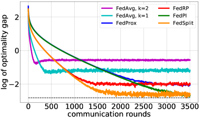
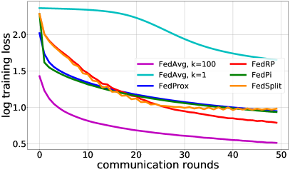
Figure 10: The effect of using minibatch gradient descent on the splitting algorithms. Local datasets are divided into $5$ minibatches. Top-Left: least squares with $B=1000$. Top-Right: logistic regression with $B=200$. Bottom: nonconvex CNN on MNIST with $B=500$.

B.5 Results with error bars: Figure 1, Left

To avoid clutter, we did not present the error bars in Figure 2 but report them here. The $y$-axis represents the training loss $\{f(\mathbf{w}_{\texttt{FedAvg}}^{*})\}$ of (approximate) fixed-point solutions of FedAvg for different learning rates $\eta$ and local epochs $k$, and the shaded area illustrates the maximum and minimum over 4 different runs.

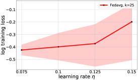
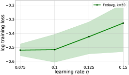
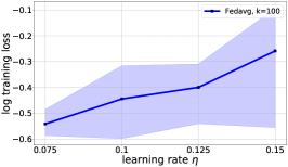
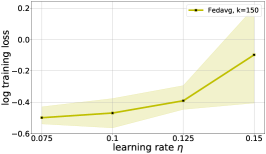
Figure 11: Nonconvex CNN on MNIST. Simulations are run for $200$ communication rounds.

B.6 Results with error bars: Figure 2, Left

Figure 12 shows the effect of step size $\eta$ and averaging on FedProx for nonconvex CNN on MNIST, and the shaded area illustrates the maximum and minimum over 4 different runs. The deviation among different runs is quite small.

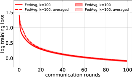
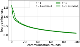
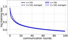
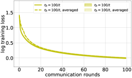
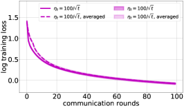
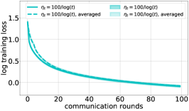
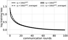
Figure 12: The dashed and solid lines with the same color show the results obtained with and without the ergodic averaging step in Theorem 2, respectively.

B.7 Results with error bars: Figure 3, Bottom

The following figures demonstrate the effect of data heterogeneity on the performance of different splitting methods for nonconvex CNN model, and the shaded area illustrates the maximum and minimum over 4 different runs.

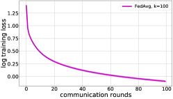
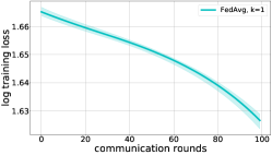
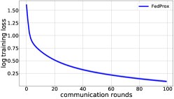
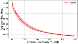
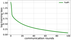
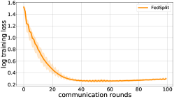
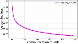
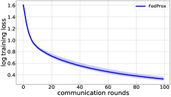
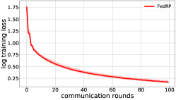
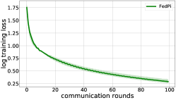
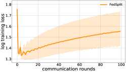
Figure 13: i.i.d. data distribution.

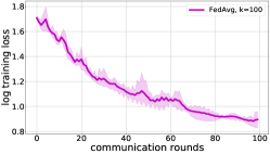
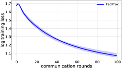
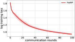
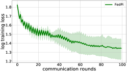
Figure 14: Non-i.i.d. data distribution with maximum $6$ classes per user.

Figure 15: Non-i.i.d. data distribution with maximum $2$ classes per user.

B.8 Results with error bars: Figure 4, Left

Implementation details of Anderson acceleration for nonconvex CNN:

In practice, we found that applying the acceleration algorithm to $\mathsf{P}_{H}(\mathsf{z}_{t+1})$ in (25) rather than $\mathsf{u}_{t+1}$ in (26) leads to a more stable algorithm. So, we applied acceleration to $\mathsf{P}_{H}(\mathsf{z}_{t+1})$, and used the result to find $\mathsf{u}_{t+1}$ and $\mathsf{w}_{t+1}$ for the nonconvex model.

Figure 16 shows the effect of Anderson acceleration on the nonconvex CNN with memory size $\tau=10$. FedRP and FedSplit are less stable and Anderson acceleration actually made them worse while FedAvg, FedProx and FedPi converge much faster with our implementation of Anderson acceleration. The deviation among 4 different runs is shown as the shaded area.

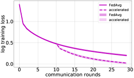
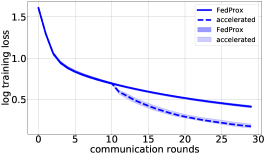
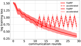
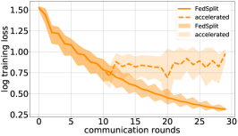
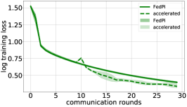
Figure 16: Nonconvex CNN with $\tau=10$. Dashed lines are the accelerated results.

Appendix C Proofs

We first recall the following convenient result:

Lemma 1 ([59], [60, Theorem 5.36]).

Let $\{\mathbf{w}_{t}\}$ and $\{\mathbf{z}_{t}\}$ be two sequences in $\mathds{R}^{d}$, $\emptyset\neq\mathsf{F}\subseteq\mathds{R}^{d}$, and $W_{k}:=\mathop{\mathrm{cl}}\mathrm{conv}\left(\mathbf{w}_{t}:t\geq k\right)$. Suppose that

1. for all $\mathbf{w}\in\mathsf{F}$, $\|\mathbf{w}_{t}-\mathbf{w}\|_{2}^{2}\to p(\mathbf{w})<\infty$;

2. for all $k$, $\mathsf{dist}(\mathbf{z}_{t},W_{k})\to 0$ as $t\to\infty$.

Then, the sequence $\{\mathbf{z}_{t}\}$ has at most one limit point in $\mathsf{F}$. Therefore, if additionally

1. all limit points of $\{\mathbf{z}_{t}\}$ lie in $\mathsf{F}$,

then the whole sequence $\{\mathbf{z}_{t}\}$ converges to a point in $\mathsf{F}$.

Below, we use well-known properties about firm nonexpansions and Fejér monotone sequences, see the excellent book [60] for background.

See 1

Proof.

The proof is a simplification and application of [61].

Consider all possible combinations of user participation, i.e. let $\mathcal{I}:=2^{[m]}\setminus\emptyset$ be the power set of users $[m]:=\{1,\ldots,m\}$, with the empty set removed. For each $I\in\mathcal{I}$, define

$$\mathsf{T}_{I}=\mathsf{T}_{I,\eta}:=\frac{1}{|I|}\sum_{i\in I}\mathsf{P}_{f_{i}}^{\eta}.$$ (28)

For any $\mathbf{w}\in\mathsf{F}$, we have $\mathbf{w}=\mathsf{P}_{f_{i}}^{\eta}\mathbf{w}$ for all $i$, and hence $\mathsf{F}\subseteq\cap_{I\in\mathcal{I}}\mathrm{Fix}\mathsf{T}_{I}$ (equality in fact when we consider singleton $I$). Moreover, since we assume each $f_{i}$ to be convex, the mapping $\mathsf{T}_{I,\eta}$ is firmly nonexpansive. In fact, $\mathsf{T}_{I,\eta}=\mathsf{P}_{f_{I}}^{\eta}$ for a so-called proximal average function $f_{I}$ [60], and hence it follows from [62] that

$$(1\wedge\eta)\|\mathbf{w}-\mathsf{T}_{I,1}\mathbf{w}\|_{2}\leq\|\mathbf{w}-\mathsf{T}_{I,\eta}\mathbf{w}\|_{2}.$$ (29)

Since we assume $\liminf_{t}\eta_{t}:=\eta>0$, the aforementioned monotonicity allows us to assume w.l.o.g. that $\eta_{t}\equiv\eta>0$.

With this established notation we rewrite FedProx simply as

$$\mathbf{w}_{t+1}=\mathsf{T}_{I_{t}}\mathbf{w}_{t},$$ (30)

where $I_{t}\in\mathcal{I}$ can be arbitrary except for all $i$, $|\{t:i\in I_{t}\}|=\infty$.

Applying the firm nonexpansiveness of $\mathsf{T}_{I_{t}}$, we have for any $\mathbf{w}\in\mathsf{F}$:

$$\|\mathbf{w}_{t+1}-\mathbf{w}\|_{2}^{2}+\|\mathbf{w}_{t}-\mathbf{w}_{t+1}\|_{2}^{2}\leq\|\mathbf{w}_{t}-\mathbf{w}\|_{2}^{2},$$ (31)

whence

$$\|\mathbf{w}_{t+1}-\mathbf{w}\|_{2}^{2}\leq\|\mathbf{w}_{t}-\mathbf{w}\|_{2}^{2},$$ (32)

i.e. $\{\mathbf{w}_{t}\}$ is Fejér monotone w.r.t. $\mathsf{F}$. Moreover,

$$\mathbf{w}_{t}-\mathsf{T}_{I_{t}}\mathbf{w}_{t}\to\mathbf{0}.$$ (33)

Since $\{\mathbf{w}_{t}\}$ is bounded and there are only finitely many choices for $I_{t}\in\mathcal{I}$, from (33) there exists $\mathbf{z}\in\cap_{J\in\mathcal{J}}\mathrm{Fix}\mathsf{T}_{J}$ that is a limit point of $\{\mathbf{w}_{t}\}$ for some $\emptyset\neq\mathcal{J}\subseteq\mathcal{I}$. Take a subsequence $\mathbf{w}_{t_{k}}\to\mathbf{z}$ and let $s_{k}=\min\{t\geq t_{k}:I_{t}\not\in\mathcal{J}\}$. Pass to a subsequence we may assume $I_{s_{k}}\equiv I$ and $\mathbf{w}_{s_{k}}\to\mathbf{w}$. Since $\mathbf{w}_{s_{k}}-\mathsf{T}_{I}\mathbf{w}_{s_{k}}\to\mathbf{0}$ (see (33)) we have $\mathbf{w}\in\mathrm{Fix}\mathsf{T}_{I}$. Since $\mathbf{z}\in\cap_{J\in\mathcal{J}}\mathrm{Fix}\mathsf{T}_{J}$ and $I_{t}\in\mathcal{J}$ for $t\in[t_{k},s_{k})$ we have

$$\|\mathbf{w}_{s_{k}}-\mathbf{z}\|_{2}\leq\|\mathbf{w}_{t_{k}}-\mathbf{z}\|_{2}\to 0,$$ (34)

and hence $\mathbf{z}=\mathbf{w}\in\mathrm{Fix}\mathsf{T}_{I}=\cap_{i\in I}\mathrm{Fix}\mathsf{P}_{f_{i}}$. Since each user $f_{i}$ participates infinitely often, we may continue the argument to conclude that any limit point $\mathbf{z}\in\mathsf{F}$. Applying Lemma 1 we know the whole sequence $\mathbf{w}_{t}\to\mathbf{w}_{\infty}\in\mathsf{F}$. ∎

We remark that the convexity condition on $f_{i}$ may be further relaxed using arguments in [63].

See 2

Proof.

We simply verify Lemma 1. Let $\mathsf{w}\in\mathop{\mathrm{dom}}\mathsf{f}\cap H$, $\mathbf{a}^{*}\in\partial\mathsf{f}(\mathsf{w})$ and $\mathbf{b}^{*}\in H^{\perp}$. Applying the firm nonexpansiveness of $\mathsf{P}_{\mathsf{f}}^{\eta_{t}}$:

$$\|\mathsf{P}_{\mathsf{f}}^{\eta_{t}}\mathsf{w}_{t}-\mathsf{w}\|_{2}^{2} =\|\mathsf{P}_{\mathsf{f}}^{\eta_{t}}\mathsf{w}_{t}-\mathsf{P}_{\mathsf{f}}^{\eta_{t}}(\mathsf{w}+\eta_{t}\mathbf{a}^{*})\|_{2}^{2}$$ (35)

$$\leq\|\mathsf{w}_{t}-\mathsf{w}-\eta_{t}\mathbf{a}^{*}\|_{2}^{2}-\|\mathsf{w}_{t}-\mathsf{P}_{\mathsf{f}}^{\eta_{t}}\mathsf{w}_{t}-\eta_{t}\mathbf{a}^{*}\|_{2}^{2}$$ (36)

$$=\|\mathsf{w}_{t}-\mathsf{w}\|_{2}^{2}-\|\mathsf{w}_{t}-\mathsf{P}_{\mathsf{f}}^{\eta_{t}}\mathsf{w}_{t}\|_{2}^{2}+2\eta_{t}\langle\mathsf{w}\!-\!\mathsf{P}_{\mathsf{f}}^{\eta_{t}}\mathsf{w}_{t};\mathbf{a}^{*}\rangle,$$ (37)

$$\|\mathsf{P}_{H}\mathsf{P}_{\mathsf{f}}^{\eta_{t}}\mathsf{w}_{t}-\mathsf{w}\|_{2}^{2} \leq\|\mathsf{P}_{\mathsf{f}}^{\eta_{t}}\mathsf{w}_{t}-\mathsf{w}\|_{2}^{2}-\|\mathsf{P}_{\mathsf{f}}^{\eta_{t}}\mathsf{w}_{t}-\mathsf{P}_{H}\mathsf{P}_{\mathsf{f}}^{\eta_{t}}\mathsf{w}_{t}\|_{2}^{2}+2\eta_{t}\langle\mathsf{w}-\mathsf{P}_{H}\mathsf{P}_{\mathsf{f}}^{\eta_{t}}\mathsf{w}_{t};\mathbf{b}^{*}\rangle.$$ (38)

Summing the above two inequalities and applying the inequality $-\|\mathbf{x}\|_{2}^{2}+2\langle\mathbf{x};\mathbf{y}\rangle\leq\|\mathbf{y}\|_{2}^{2}$ repeatedly:

$$\|\mathsf{P}_{H}\mathsf{P}_{\mathsf{f}}^{\eta_{t}}\mathsf{w}_{t}-\mathsf{w}\|_{2}^{2}\leq\|\mathsf{w}_{t}-\mathsf{w}\|_{2}^{2}+2\eta_{t}\langle\mathsf{w}-\mathsf{w}_{t};\mathbf{a}^{*}+\mathbf{b}^{*}\rangle+\eta_{t}^{2}[\|\mathbf{a}^{*}+\mathbf{b}^{*}\|_{2}^{2}+\|\mathbf{a}^{*}\|^{2}_{2}].$$ (39)

Summing over $t$ and rearranging we obtain for any $\mathsf{w}\in\mathop{\mathrm{dom}}\mathsf{f}\cap H,\mathsf{w}^{*}=\mathbf{a}^{*}+\mathbf{b}^{*}$:

$$2\langle\mathsf{w}-\bar{\mathsf{w}}_{t};\mathsf{w}^{*}\rangle+[\|\mathbf{a}^{*}\|_{2}^{2}+\|\mathsf{w}^{*}\|_{2}^{2}]\sum_{k=0}^{t}\eta_{k}^{2}/\Lambda_{t}\geq(\|\mathsf{w}_{t+1}-\mathsf{w}\|_{2}^{2}-\|\mathsf{w}_{1}-\mathsf{w}\|_{2}^{2})/\Lambda_{t},$$ (40)

where $\Lambda_{t}:=\sum_{k=1}^{t}\eta_{k}$. Using the assumptions on $\eta_{t}$ we thus know

$$\liminf_{t\to\infty}\leavevmode\nobreak\ \leavevmode\nobreak\ \langle\mathsf{w}-\bar{\mathsf{w}}_{t};\mathsf{w}^{*}\rangle\geq 0.$$ (41)

Since $\mathsf{w}$ is arbitrary and $\mathsf{w}^{*}$ is chosen to be its subdifferential, it follows that any limit point of $\{\bar{\mathsf{w}}_{t}\}$ is a solution of the original problem (1), i.e. condition 3 of Lemma 1 holds. If $\{\bar{\mathsf{w}}_{t}\}$ is bounded, then $\mathsf{F}\neq\emptyset$, which we assume now. Let $\mathsf{w}\in\mathsf{F}$ and set $\mathsf{w}^{*}=\mathbf{0}$ we know from (39) that $\{\mathsf{w}_{t}\}$ is quasi-Fejér monotone w.r.t. $\mathsf{F}$ (i.e. condition 1 in Lemma 1 holds). Lastly, let $\bar{\eta}_{t,k}:=\eta_{k}/\Lambda_{t}$ and we verify condition (II) in Lemma 1:

$$\mathsf{dist}(\bar{\mathsf{w}}_{t},W_{k}) \leq\left\|\bar{\mathsf{w}}_{t}-\sum_{s=k}^{t}\bar{\eta}_{t,s}\mathsf{w}_{s}/\sum_{\kappa=k}^{t}\bar{\eta}_{t,\kappa}\right\|_{2}$$ (42)

$$\leq\sum_{\kappa=0}^{k-1}\bar{\eta}_{t,\kappa}\left[\|\mathsf{w}_{\kappa}\|_{2}+\left\|\sum_{s=k}^{t}\bar{\eta}_{t,s}\mathsf{w}_{s}\right\|_{2}/\sum_{\kappa=k}^{t}\bar{\eta}_{t,\kappa}\right]$$ (43)

$$\stackrel{{\scriptstyle t\to\infty}}{{\longrightarrow}}0,$$ (44)

since $\mathsf{w}_{t}$ is bounded and for any $k$, $\bar{\eta}_{t,k}\to 0$ as $t\to\infty$. All three conditions in Lemma 1 are now verified. ∎

We remark that the step size condition is tight, as shown by the following simple example:

Example 1.

Let $f_{\pm}(w)=\tfrac{1}{2}(w\pm 1)^{2}$. Simple calculation verifies that

$$\mathsf{P}_{f_{\pm}}^{\eta}(w)=\tfrac{w\mp\eta}{1+\eta}.$$ (45)

Therefore, the iterates of FedProx for the two functions $f_{+}$ and $f_{-}$ are:

$$w_{t+1}=\tfrac{w_{t}}{1+\eta_{t}}=\prod_{\tau=0}^{t}\tfrac{1}{1+\eta_{\tau}}w_{0},$$ (46)

which tends to the true minimizer $w_{\star}=0$ for any $w_{0}$ iff

$$\prod_{\tau=0}^{t}\tfrac{1}{1+\eta_{\tau}}\to 0\iff\sum_{t}\eta_{t}\to\infty.$$ (47)

If we consider instead $f_{+}$ and $2f_{-}$, then

$$2w_{t+1}=\tfrac{w_{t}-\eta_{t}}{1+\eta_{t}}+\tfrac{w_{t}+2\eta_{t}}{1+2\eta_{t}}.$$ (48)

Passing to a subsequence if necessary, let $\eta_{t}\to\eta\neq 0$ and suppose $w_{t}\to w_{\star}=\tfrac{1}{3}$, then passing to the limit we obtain

$$2=\tfrac{1-3\eta}{1+\eta}+\tfrac{1+6\eta}{1+2\eta} \iff 2(1+\eta)(1+2\eta)=(1-3\eta)(1+2\eta)+(1+6\eta)(1+\eta)$$ (49)

$$\iff\eta=0,$$ (50)

contradiction. Therefore, it is necessary to have $\eta_{t}\to 0$ in order for FedProx to converge to the true solution $w_{\star}=\tfrac{1}{3}$ on this example.

See 5

Proof.

Since $\mathsf{R}_{f}^{\eta}=\mathsf{R}_{\eta f}$ and $f$ is strongly convex iff $\eta f$ is so, w.l.o.g. we may take $\eta=1$. Suppose $\mathsf{R}_{f}$ is $\gamma$-contractive for some $\gamma\in(0,1)$, i.e. for all $\mathbf{w}$ and $\mathbf{z}$:

$$\|\mathsf{R}_{f}\mathbf{w}-\mathsf{R}_{f}\mathbf{z}\|_{2}\leq\gamma\cdot\|\mathbf{w}-\mathbf{z}\|_{2}.$$ (51)

It then follows that the proximal map $\mathsf{P}_{f}=\tfrac{\mathrm{id}+\mathsf{R}_{f}}{2}$ is $\tfrac{1+\gamma}{2}$-contractive. Moreover, $\tfrac{2}{1+\gamma}\mathsf{P}_{f}$, being nonexpansive, is the gradient of the convex function $\tfrac{2}{1+\gamma}\mathsf{M}_{f^{*}}$. Thus, $\tfrac{2}{1+\gamma}\mathsf{P}_{f}$ is actually firmly nonexpansive [60, Corollary 18.17]. But,

$$\tfrac{2}{1+\gamma}\mathsf{P}_{f}=\tfrac{2}{1+\gamma}(\mathrm{id}+\partial f)^{-1}=[\mathrm{id}+(\partial f-\tfrac{1-\gamma}{1+\gamma}\mathrm{id})\circ\tfrac{1+\gamma}{2}\mathrm{id}]^{-1},$$ (52)

and hence $(\partial f-\tfrac{1-\gamma}{1+\gamma}\mathrm{id})\circ\tfrac{1+\gamma}{2}\mathrm{id}$ is maximal monotone [60, Proposition 23.8], i.e. $f$ is $\tfrac{1-\gamma}{1+\gamma}$-strongly convex. ∎

See 7

Proof.

To see the first claim, let $\mathsf{w}$ be a fixed point of FedRP, i.e.

$$\mathsf{w}=\mathsf{P}_{H}\mathsf{R}_{\mathsf{f}}^{\eta}\mathsf{w}=\mathsf{P}_{H}(2\mathsf{P}_{\mathsf{f}}^{\eta}\mathsf{w}-\mathsf{w})=2\mathsf{P}_{H}\mathsf{P}_{\mathsf{f}}^{\eta}\mathsf{w}-\mathsf{P}_{H}\mathsf{w}=2\mathsf{P}_{H}\mathsf{P}_{\mathsf{f}}^{\eta}\mathsf{w}-\mathsf{w},$$ (53)

since $\mathsf{P}_{H}$ is linear and $\mathsf{w}\in H$ due to the projection. Thus, $\mathsf{w}=\mathsf{P}_{H}\mathsf{P}_{\mathsf{f}}^{\eta}\mathsf{w}$. In other words, the fixed points of FedRP are exactly those of FedProx, and the first claim then follows from [51], see the discussions in Section 3.2 and also [39, Lemma 7.1].

To prove the second claim, we first observe that $\{\mathsf{w}_{t}\}$ is Fejér monotone w.r.t. $\mathsf{F}$, the solution set of the regularized problem (13). Indeed, for any $\mathsf{w}\in\mathsf{F}$, using the firm nonexpansiveness of $\mathsf{P}_{H}$ we have

$$\|\mathsf{w}_{t+1}-\mathsf{w}\|_{2}^{2}+\|\mathsf{R}_{\mathsf{f}}^{\eta}\mathsf{w}_{t}-\mathsf{w}_{t+1}-\mathsf{R}_{\mathsf{f}}^{\eta}\mathsf{w}+\mathsf{w}\|_{2}^{2}\leq\|\mathsf{R}_{\mathsf{f}}^{\eta}\mathsf{w}_{t}-\mathsf{R}_{\mathsf{f}}^{\eta}\mathsf{w}\|_{2}^{2}\leq\|\mathsf{w}_{t}-\mathsf{w}\|_{2}^{2}.$$ (54)

Summing and telescoping the above we know

$$\mathsf{R}_{\mathsf{f}}^{\eta}\mathsf{w}_{t}-\mathsf{w}_{t+1}\to\mathsf{R}_{\mathsf{f}}^{\eta}\mathsf{w}-\mathsf{w}.$$ (55)

Let $\mathsf{w}_{\infty}$ be a limit point of $\{\mathsf{w}_{t}\}$ (which exists since $\mathsf{w}_{t}$ is bounded). Since $\mathsf{R}_{\mathsf{f}}^{\eta}$ is idempotent, we have the range $\mathop{\mathrm{rge}}\mathsf{R}_{\mathsf{f}}^{\eta}$ equal to its fixed point $\mathrm{Fix}\mathsf{R}_{\mathsf{f}}^{\eta}$. When the users are homogeneous, we can choose $\mathsf{w}=\mathsf{R}_{\mathsf{f}}^{\eta}\mathsf{w}$. Therefore, $\mathsf{w}_{\infty}\in\mathop{\mathrm{rge}}\mathsf{R}_{\mathsf{f}}=\mathrm{Fix}\mathsf{R}_{\mathsf{f}}$. Since $\mathbf{w}_{\infty}\in H$ by definition, $\mathbf{w}_{\infty}\in\mathsf{F}$. Applying Lemma 1 we conclude that the entire Fejér sequence $\{\mathsf{w}_{t}\}$ converges to $\mathbf{w}_{\infty}\in\mathsf{F}$. ∎

As shown in [39], a (closed) convex cone is obtuse iff its reflector is idempotent. To give another example: the univariate, idempotent reflector $\mathsf{R}_{f}(w)=(w)_{+}:=\max\{w,0\}$ leads to

$$\mathsf{P}_{f}(w)=\tfrac{w+\mathsf{R}_{f}w}{2}=\tfrac{w+(w)_{+}}{2}\implies f(w)=\tfrac{1}{2}(-w)_{+}^{2}.$$ (56)

Interestingly, the epigraph of the above $f$ is a convex set but not a cone and yet its reflector is idempotent. Therefore, the idempotent condition introduced here is a strict generalization of [39].

References

- [1] Brendan McMahan, Eider Moore, Daniel Ramage, Seth Hampson and Blaise Agüera Arcas “Communication-Efficient Learning of Deep Networks from Decentralized Data” In AISTATS 54, 2017, pp. 1273–1282 URL: http://proceedings.mlr.press/v54/mcmahan17a/mcmahan17a.pdf
- [2] Tian Li et al. “Federated Optimization in Heterogeneous Networks” In Proceedings of Machine Learning and Systems 2, 2020, pp. 429–450 URL: https://proceedings.mlsys.org/paper/2020/file/38af86134b65d0f10fe33d30dd76442e-Paper.pdf
- [3] Mikhail Yurochkin et al. “Bayesian Nonparametric Federated Learning of Neural Networks” In ICML 97, 2019, pp. 7252–7261 URL: http://proceedings.mlr.press/v97/yurochkin19a.html
- [4] Sashank Reddi et al. “Adaptive Federated Optimization” arXiv:2003.00295, 2020 URL: https://arxiv.org/abs/2003.00295
- [5] Reese Pathak and Martin J. Wainwright “FedSplit: An algorithmic framework for fast federated optimization” In NeurIPS, 2020 URL: https://proceedings.neurips.cc//paper/2020/hash/4ebd440d99504722d80de606ea8507da-Abstract.html
- [6] Zhouyuan Huo, Qian Yang, Bin Gu, Lawrence Carin and Heng Huang “Faster On-Device Training Using New Federated Momentum Algorithm” arXiv:2002.02090, 2020 URL: https://arxiv.org/abs/2002.02090
- [7] Hongyi Wang, Mikhail Yurochkin, Yuekai Sun, Dimitris Papailiopoulos and Yasaman Khazaeni “Federated Learning with Matched Averaging” In ICLR, 2020 URL: https://openreview.net/forum?id=BkluqlSFDS
- [8] Zhize Li, Dmitry Kovalev, Xun Qian and Peter Richtárik “Acceleration for Compressed Gradient Descent in Distributed and Federated Optimization” In ICML, 2020, pp. 5895–5904 URL: http://proceedings.mlr.press/v119/li20g.html
- [9] Ahmed Khaled, Konstantin Mishchenko and Peter Richtárik “First Analysis of Local GD on Heterogeneous Data” arXiv:1909.04715, 2020 URL: https://arxiv.org/abs/1909.04715
- [10] Xiang Li, Kaixuan Huang, Wenhao Yang, Shusen Wang and Zhihua Zhang “On the Convergence of FedAvg on Non-IID Data” In ICLR, 2020 URL: https://openreview.net/forum?id=HJxNAnVtDS
- [11] Ahmed Khaled, Konstantin Mishchenko and Peter Richtarik “Tighter Theory for Local SGD on Identical and Heterogeneous Data” In AISTATS 108, 2020, pp. 4519–4529 URL: http://proceedings.mlr.press/v108/bayoumi20a.html
- [12] Grigory Malinovskiy, Dmitry Kovalev, Elnur Gasanov, Laurent Condat and Peter Richtarik “From Local SGD to Local Fixed-Point Methods for Federated Learning” In ICML 119, 2020, pp. 6692–6701 URL: http://proceedings.mlr.press/v119/malinovskiy20a.html
- [13] Eduard Gorbunov, Filip Hanzely and Peter Richtárik “Local SGD: Unified theory and new efficient methods” In AISTATS 130, 2021, pp. 3556–3564 URL: http://proceedings.mlr.press/v130/gorbunov21a.html
- [14] Yishay Mansour, Mehryar Mohri, Jae Ro and Ananda Theertha Suresh “Three Approaches for Personalization with Applications to Federated Learning” arXiv:2002.10619, 2020 URL: https://arxiv.org/abs/2002.10619
- [15] Canh T. Dinh, Nguyen Tran and Josh Nguyen “Personalized Federated Learning with Moreau Envelopes” In NeurIPS, 2020, pp. 21394–21405 URL: https://proceedings.neurips.cc/paper/2020/file/f4f1f13c8289ac1b1ee0ff176b56fc60-Paper.pdf
- [16] Enmao Diao, Jie Ding and V. Tarokh “HeteroFL: Computation and Communication Efficient Federated Learning for Heterogeneous Clients” In ICLR, 2021 URL: https://openreview.net/forum?id=TNkPBBYFkXg
- [17] Michael Zhang, Karan Sapra, S. Fidler, Serena Yeung and Jose M. Alvarez “Personalized Federated Learning with First Order Model Optimization” In ICLR, 2021 URL: https://openreview.net/forum?id=ehJqJQk9cw
- [18] Yuyang Deng, Mohammad Mahdi Kamani and M. Mahdavi “Adaptive Personalized Federated Learning” In ArXiv abs/2003.13461, 2020 URL: https://arxiv.org/pdf/2003.13461
- [19] M. Nasr, R. Shokri and A. Houmansadr “Comprehensive Privacy Analysis of Deep Learning: Passive and Active White-box Inference Attacks against Centralized and Federated Learning” In IEEE Symposium on Security and Privacy (SP), 2019, pp. 739–753 URL: 10.1109/SP.2019.00065
- [20] Sean Augenstein et al. “Generative Models for Effective ML on Private, Decentralized Datasets” In ICLR, 2020 URL: https://openreview.net/forum?id=SJgaRA4FPH
- [21] Arjun Nitin Bhagoji, Supriyo Chakraborty, Prateek Mittal and Seraphin Calo “Analyzing Federated Learning through an Adversarial Lens” In ICML 97, 2019, pp. 634–643 URL: http://proceedings.mlr.press/v97/bhagoji19a.html
- [22] Eugene Bagdasaryan, Andreas Veit, Yiqing Hua, Deborah Estrin and Vitaly Shmatikov “How To Backdoor Federated Learning” In AISTATS 108, 2020, pp. 2938–2948 URL: http://proceedings.mlr.press/v108/bagdasaryan20a.html
- [23] Ziteng Sun, Peter Kairouz, Ananda Theertha Suresh and H Brendan McMahan “Can You Really Backdoor Federated Learning?” arXiv:1911.07963, 2019 URL: https://arxiv.org/abs/1911.07963
- [24] Amirhossein Reisizadeh, Farzan Farnia, Ramtin Pedarsani and Ali Jadbabaie “Robust Federated Learning: The Case of Affine Distribution Shifts” In NeurIPS, 2020 URL: https://proceedings.neurips.cc/paper/2020/file/f5e536083a438cec5b64a4954abc17f1-Paper.pdf
- [25] Zeou Hu, Kiarash Shaloudegi, Guojun Zhang and Yaoliang Yu “FedMGDA+: Federated Learning meets Multi-objective Optimization” arXiv:2006.11489, 2020 URL: https://arxiv.org/abs/2006.11489
- [26] Mehryar Mohri, Gary Sivek and Ananda Theertha Suresh “Agnostic Federated Learning” In ICML 97, 2019, pp. 4615–4625 URL: http://proceedings.mlr.press/v97/mohri19a.html
- [27] Tian Li, Maziar Sanjabi, Ahmad Beirami and Virginia Smith “Fair Resource Allocation in Federated Learning” In ICLR, 2020 URL: https://openreview.net/forum?id=ByexElSYDr
- [28] Sebastian Caldas et al. “Leaf: A benchmark for federated settings” arXiv:1812.01097, 2018 URL: https://arxiv.org/abs/1812.01097
- [29] Chaoyang He et al. “FedML: A research library and benchmark for federated machine learning” arXiv:2007.13518, 2020 URL: https://arxiv.org/abs/2007.13518
- [30] Virginia Smith, Chao-Kai Chiang, Maziar Sanjabi and Ameet S. Talwalkar “Federated Multi-Task Learning” In NeurIPS, 2017 URL: https://papers.nips.cc/paper/2017/hash/6211080fa89981f66b1a0c9d55c61d0f-Abstract.html
- [31] Peter Kairouz et al. “Advances and Open Problems in Federated Learning” arXiv:1912.04977, 2019 URL: https://arxiv.org/abs/1912.04977
- [32] Tian Li, Anit Kumar Sahu, Ameet Talwalkar and Virginia Smith “Federated learning: Challenges, methods, and future directions” arXiv:1908.07873, 2019 URL: https://arxiv.org/abs/1908.07873
- [33] Qiang Yang, Yang Liu, Tianjian Chen and Yongxin Tong “Federated Machine Learning: Concept and Applications” In ACM Transactions on Intelligent Systems and Technology 10.2, 2019 URL: https://doi.org/10.1145/3298981
- [34] Zachary Charles and Jakub Konečný “Convergence and Accuracy Trade-Offs in Federated Learning and Meta-Learning” In AISTATS, 2021 URL: http://proceedings.mlr.press/v130/charles21a/charles21a.pdf
- [35] D.. Peaceman and H.. Rachford “The Numerical Solution of Parabolic and Elliptic Differential Equations” In Journal of the Society for Industrial and Applied Mathematics 3.1, 1955, pp. 28–41 URL: https://www.jstor.org/stable/2098834
- [36] Pierre-Louis Lions and B. Mercier “Splitting Algorithms for the Sum of Two Nonlinear Operators” In SIAM Journal on Numerical Analysis 16.6, 1979, pp. 964–979 URL: https://doi.org/10.1137/0716071
- [37] Jim Douglas and H.. Rachford “On the Numerical Solution of Heat Conduction Problems in Two and Three Space Variables” In Transactions of the American Mathematical Society 82.2, 1956, pp. 421–439 URL: https://doi.org/10.2307/1993056
- [38] Jonathan E. Spingarn “Applications of the method of partial inverses to convex programming: Decomposition” In Mathematical Programming 32, 1985, pp. 199–223 URL: https://doi.org/10.1007/BF01586091
- [39] H.. Bauschke and S.. Kruk “Reflection-Projection Method for Convex Feasibility Problems with an Obtuse Cone” In Journal of Optimization Theory and Applications 120.3, 2004, pp. 503–531 URL: https://doi.org/10.1023/B:JOTA.0000025708.31430.22
- [40] Donald G. Anderson “Iterative Procedures for Nonlinear Integral Equations” In Journal of ACM 12.4, 1965, pp. 547–560 URL: https://doi.org/10.1145/321296.321305
- [41] Anqi Fu, Junzi Zhang and Stephen Boyd “Anderson Accelerated Douglas–Rachford Splitting” In SIAM Journal on Scientific Computing 42.6, 2020, pp. A3560–A3583 URL: https://doi.org/10.1137/19M1290097
- [42] Ronald E. Bruck “On the weak convergence of an ergodic iteration for the solution of variational inequalities for monotone operators in Hilbert space” In Journal of Mathematical Analysis and Applications 61.1, 1977, pp. 159–164 URL: https://doi.org/10.1016/0022-247X(77)90152-4
- [43] Yann LeCun, Corinna Cortes and CJ Burges “MNIST handwritten digit database” Available Under the Terms of the Creative Commons Attribution-Share Alike 3.0 License In ATT Labs [Online] 2, 2010 URL: http://yann.lecun.com/exdb/mnist
- [44] Pierre-Louis Lions “Une methode iterative de resolution d’une inequation variationnelle” In Israel Journal of Mathematics 31.2, 1978, pp. 204–208 URL: https://doi.org/10.1007/BF02760552
- [45] Gregory B. Passty “Ergodic convergence to a zero of the sum of monotone operators in Hilbert space” In Journal of Mathematical Analysis and Applications 72.2, 1979, pp. 383–390 URL: https://doi.org/10.1016/0022-247X(79)90234-8
- [46] Gianfranco Cimmino “Calcolo Approssimato Per le Soluzioni dei Sistemi di Equazioni Lineari” In La Ricerca Scientifica, Series II 9, 1938, pp. 326–333
- [47] Jacques Louis Lions and Roger Temam “Une méthode d’éclatement pes opérateurs et des contraintes en calcul des variations” In Comptes rendus mathématiques de l’Académie des Sciences, Paris 263, 1966, pp. 563–565 URL: https://gallica.bnf.fr/ark:/12148/bpt6k6426017v/f241
- [48] Alfred Auslender “Méthodes Numériques pour la Résolution des Problèmes d’Optimisation avec Contraintes”, 1969
- [49] Yaoliang Yu “Better Approximation and Faster Algorithm Using the Proximal Average” In NeurIPS, 2013 URL: https://proceedings.neurips.cc/paper/2013/hash/49182f81e6a13cf5eaa496d51fea6406-Abstract.html
- [50] Yaoliang Yu, Xun Zheng, Micol Marchetti-Bowick and Eric P. Xing “Minimizing Nonconvex Non-Separable Functions” In AISTATS 38, 2015, pp. 1107–1115 URL: http://proceedings.mlr.press/v38/yu15.html
- [51] Heinz H. Bauschke, Patrick L. Combettes and Simeon Reich “The asymptotic behavior of the composition of two resolvents” In Nonlinear Analysis: Theory, Methods & Applications 60.2, 2005, pp. 283–301 URL: https://doi.org/10.1016/j.na.2004.07.054
- [52] R. Rockafellar and Roger J-B Wets “Variational Analysis” Springer, 1998 URL: https://link.springer.com/book/10.1007/978-3-642-02431-3
- [53] Daniel Gabay “Applications of the Method of Multipliers to Variational Inequalities” In Augmented Lagrangian methods: Applications to the numerical solution of boundary-value problems 15, 1983, pp. 299–331 URL: https://doi.org/10.1016/S0168-2024(08)70034-1
- [54] Jonathan E. Spingarn “Partial inverse of a monotone operator” In Applied Mathematics and Optimization 10, 1983, pp. 247–265 URL: https://doi.org/10.1007/BF01448388
- [55] R. Rockafellar “Progressive Decoupling of Linkages in Optimization and Variational Inequalities with Elicitable Convexity or Monotonicity” In Set-Valued and Variational Analysis 27, 2019, pp. 863–893 URL: https://doi.org/10.1007/s11228-018-0496-1
- [56] Andreas Themelis and Panagiotis Patrinos “Douglas–Rachford Splitting and ADMM for Nonconvex Optimization: Tight Convergence Results” In SIAM Journal on Optimization 30.1, 2020, pp. 149–181 URL: https://doi.org/10.1137/18M1163993
- [57] Jonathan Eckstein and Dimitri P. Bertsekas “On the Douglas—Rachford splitting method and the proximal point algorithm for maximal monotone operators” In Mathematical Programming 55, 1992, pp. 293–318 URL: https://doi.org/10.1007/BF01581204
- [58] Junzi Zhang, Brendan O’Donoghue and Stephen Boyd “Globally Convergent Type-I Anderson Acceleration for Nonsmooth Fixed-Point Iterations” In SIAM Journal on Optimization 30.4, 2020, pp. 3170–3197 URL: https://doi.org/10.1137/18M1232772
- [59] H. Brézis and F.. Browder “Nonlinear ergodic theorems” In Bulletin of the American Mathematical Society 82.6, 1976, pp. 959–961 URL: https://projecteuclid.org:443/euclid.bams/1183538367
- [60] Heinz H. Bauschke and Patrick L. Combettes “Convex Analysis and Monotone Operator Theory in Hilbert Spaces” Springer, 2017 URL: https://link.springer.com/book/10.1007/978-3-319-48311-5
- [61] Paul Tseng “On the Convergence of the Products of Firmly Nonexpansive Mappings” In SIAM Journal on Optimization 2.3, 1992, pp. 425–434 URL: https://doi.org/10.1137/0802021
- [62] Paul Tseng “A Modified Forward-Backward Splitting Method for Maximal Monotone Mappings” In SIAM Journal on Control and Optimization 38.2, 2000, pp. 431–446 URL: https://doi.org/10.1137/S0363012998338806
- [63] Arkady Aleyner and Simeon Reich “Random Products of Quasi-Nonexpansive Mappings in Hilbert Space” In Journal of Convex Analysis 16.3, 2009, pp. 633–640 URL: https://www.heldermann.de/JCA/JCA16/JCA163/jca16036.htm