Fully localised three-dimensional gravity-capillary solitary waves on water of infinite depth
B. Buffoni
Institut de mathématiques, Station 8, École polytechnique fédérale, 1015 Lausanne, Switzerland
M. D. Groves111Fachrichtung Mathematik, Universität des Saarlandes,
Postfach 151150, 66041 Saarbrücken, GermanyE. Wahlén222Centre for Mathematical Sciences, Lund University, PO Box 118, 22100 Lund, Sweden
Abstract
Fully localised solitary waves are travelling-wave solutions
of the three-dimensional gravity-capillary water wave problem which
decay to zero in every horizontal spatial direction. Their existence for
water of finite depth has recently been established, and in this article
we present an existence theory for water of infinite depth. The governing
equations are reduced to a perturbation of the two-dimensional
nonlinear Schrödinger equation, which admits a family
of localised solutions. Two of these solutions are symmetric in both
horizontal directions and an application of a suitable version of the
implicit-function theorem shows that they persist under perturbations.
1 Introduction
Three-dimensional gravity-capillary water waves on the surface of
a body of water of infinite depth are described by the Euler equations
in a domain bounded above by a free
surface , where the
function depends upon the two horizontal spatial directions
, and time .
In terms of an Eulerian velocity potential and in dimensionless coordinates,
the mathematical problem is to solve Laplace’s equation
(1.1)
with boundary conditions
(1.2)
(1.3)
and
(1.4)
In this article we consider fully localised solitary waves, that is nontrivial
travelling-wave solutions to (1.1)–(1.4) of the form
,
(so that the waves move with unchanging shape and constant speed from left to right)
with as (so that the waves
decay in every horizontal direction).
Theorem 1.1.
Suppose that . For each sufficiently small value of
there exist two solitary-wave solutions
of (1.1)–(1.4) for which is
symmetric in and and given by
uniformly over , where is the unique
symmetric, positive (real) solution of the two-dimensional nonlinear Schrödinger equation
(1.5)
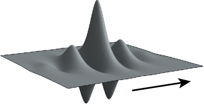
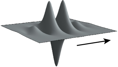
This result confirms the prediction made on the basis of model equations (see below) and
numerical computations by Parau, Vanden-Broeck & Cooker [11]
(see Figure 1 for sketches of typical free surfaces in their simulations). Qualitative
properties of (two- and three-dimensional) solitary waves on deep water have been discussed
by Wheeler [15].
Figure 1: Sketch of a symmetric fully localised solitary wave of elevation (left) and depression (right); the
arrow shows the direction of wave propagation.
We proceed by formulating the water-wave problem (1.1)–(1.4)
in terms of the variables and (see Zakharov [16] and
Craig & Sulem [5]). The Zakharov-Craig-Sulem formulation of the water-wave problem is
where and
is the (unique) solution of the boundary-value problem
Travelling waves are solutions of the form , ; they satisfy
(1.6)
(1.7)
Equations (1.6), (1.7) can be reduced to a single equation
for . Using (1.6), one finds that , and inserting this formula into
(1.7) yields the equation
(1.8)
where
(1.9)
(1.10)
and
Note the equivalent definitions
(1.11)
where is the solution of the boundary-value problem
(1.12)
(1.13)
(1.14)
(which is unique up to an additive constant); the operators and are studied in Section 2 below.
Although this fact is not used in the present paper, let us note that (1.8) is in fact the Euler-Lagrange equation for the functional
where
the functions and are the -gradients of respectively
and (see Buffoni et al. [2, 3]).
Finally, observe that equation (1.8) is invariant under the reflections
and ; a solution which is invariant
under these transformations is termed symmetric.
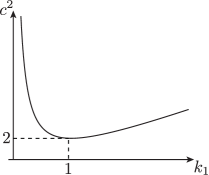
Figure 2: Dispersion relation for a two-dimensional travelling wave train
with wave number and speed .
It is instructive to review the formal derivation of the nonlinear Schrödinger equation for travelling waves
(see Ablowitz & Segur [1, §2.2]),
beginning with sinusoidal wave trains.
The linearised version of (1.8) admits a solution
of the form
whenever and satisfy the linear dispersion relation
(see Figure 2); note that the function ,
has a unique global minimum at .
Bifurcations of nonlinear solitary waves are expected whenever the
linear group and phase speeds are equal, so that (see Dias & Kharif [6, §3]).
We therefore expect the existence of small-amplitude solitary waves with speed near ;
the waves bifurcate from a linear sinusoidal wave train with unit wavenumber.
Substituting and the Ansatz
where , ,
into equation (1.8), one finds that satisfies the stationary nonlinear Schrödinger equation
(1.5).
This equation has a unique symmetric, positive (real) solution which is characterised as the ground state of
the functional with
(see Sulem & Sulem [13, §4.2] and the references therein).
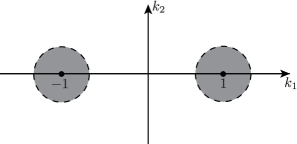
Figure 3: The support of is contained in the set .
The above Ansatz suggests that the Fourier transform of a fully localised solitary wave
is concentrated near the points and . We therefore decompose into the sum of functions
and whose Fourier transforms
and are supported in
the region (with ) and its complement (see Figure 3).
(The Fourier transform is defined by the formula
and we use the notation with for the Fourier multiplier-operator with symbol , so that
; in particular ,
, where is the characteristic function of the set .)
Writing and
decomposing (1.8) into
one finds that the second equation can be solved for as a function of for sufficiently
small values of ; substituting
into the first yields the reduced equation
for . Finally, the scaling
(1.15)
transforms the reduced equation into a perturbation of the equation
(1.16)
where and
(see Sections 3 and 4; the reduced equation is stated precisely in equation (4.2)).
Equation (1.16) is termed a full-dispersion
version of the stationary nonlinear Schrödinger equation (1.5) since it retains the linear part of the original equation
(1.8);
noting that
we obtain the fully reduced model equation
in the formal limit
(see Obrecht & Saut [10] for a discussion of related full-dispersion model equations for
three-dimensional water waves).
The existence theory is completed in Section 5, where we
exploit the fact that the reduction procedure preserves the invariance
of equation (1.8) under
and , so that equation (1.16) is
invariant under the reflections and .
We demonstrate that the reduced equation for has two symmetric solutions
which satisfy in as . The key step is a nondegeneracy result for the solution of (1.5)
(see Weinstein [14], Kwong [9] and
Chang et al. [4]) in a symmetric setting
which allows one to apply a suitable version of the implicit-function theorem.
A similar method was recently used by Stefanov & Wright [12] to establish the existence of
solitary-wave solutions to the Whitham equation (a full-dispersion Korteweg-de Vries equation).
The scaling (1.15) implies that our waves have small amplitude but finite energy.
When splitting our basic function space
into two parts , for and ,
we respect this scaling by equipping with the scaled norm defined by
(1.17)
and taking in a ball which is large enough to contain ; solving
the equation for yields the estimate
where is a fixed number in the interval . Equation (1.17) shows that our waves have finite -norm, while the estimates
shows that they have small amplitude.
Our result complements recent existence theories for fully localised gravity-capillary solitary waves on
water of finite depth (Groves & Sun [7] and Buffoni et al. [2, 3]), which also confirm predictions made
by model equations, namely the KP-I equation for ‘strong’ and Davey-Stewartson equation
for ‘weak’ surface tension (see Ablowitz & Segur [1]). In particular,
Buffoni et al. [3] present a variational counterpart of the
theory in the present paper by reducing a classical variational principle for fully localised solitary waves
to a locally equivalent variational principle featuring a perturbation of the functional associated with the
Davey-Stewartson equation. A nontrivial critical point of the reduced functional is found by showing
that an appropriate direct method for the Davey-Stewartson functional (minimisation over its natural constraint set)
is robust under perturbation. This variational method is also applicable here, allowing one to reduce the
functional to a perturbation of the functional . The present method however has the
advantages of being more explicit and yielding two distinct families of fully localised solitary waves.
2 Analyticity
In this section we show that the operators , given by (1.11)
and hence and given by (1.9), (1.10) are analytic
at the origin in suitable function spaces (see Corollaries 2.2 and 2.3 below).
The boundary-value problem (1.12)–(1.14) is handled using the change of variable
which maps to the lower half-space
.
Dropping the primes, one finds that (1.12)–(1.14) are transformed into
(2.1)
(2.2)
(2.3)
where
and , . We study this boundary-value problem in the space
for and for , in which
, , is the completion of
with respect to the norm
and denotes the usual norm for the standard Sobolev space or .
Lemma 2.1.
For each and sufficiently small
the boundary-value problem (2.1)–(2.3) admits a unique solution
.
Furthermore, the mapping defines a function
which is analytic at the origin.
Proof.
First note that for each , , and the boundary-value problem
admits a unique solution in whose gradient is obtained from the explicit formula
(with a slight abuse of notation), so that
Define
by
and note that the solutions of (2.1)–(2.3) are precisely the zeros of .
Using the estimates
and similarly
(where we have used the fact that has compact support), we find
that the mappings given by
, ,
are analytic at the origin; it follows that is also analytic at the origin.
Furthermore and
is an isomorphism.
By the analytic implicit-function theorem there exist open neighbourhoods and of the origin in
and and an analytic function
such that
Since is linear in one can take to be the entire space .∎
Corollary 2.2.
The mappings
are analytic at the origin.
In view of Corollary 2.2 we choose sufficiently small and study the equation
(2.4)
in the set
noting that is continuously embedded in and that is an open neighbourhood of the origin in ;
we proceed accordingly by decomposing into the direct sum of
and .
Corollary 2.3.
The formulae (1.9), (1.10)
define functions
which are analytic at the origin and satisfy .
Proof.
The result for follows from (1.9), Corollary 2.2 and the fact that
is an algebra. The result for follows from (1.10) and the observation that
and
define functions which are analytic at the origin since is an
algebra.∎
In keeping with Lemma 2.1 and Corollary 2.2 we write
where is homogeneous of degree in and linear in , and
where , and , are homogeneous of degree in .
A straightforward calculation shows that
and hence that and are Fourier-multiplier operators, namely
(we have omitted the argument on the left-hand sides of these equations).
The following lemma gives
expressions for the first few terms in the Maclaurin expansions of and ;
it is proved by expanding (1.9), (1.10) and
examining the boundary-value problems for and to derive
the formulae
(2.5)
(2.6)
with a similar formula for (see Buffoni et al. [2, pp. 1032–1033] for details in a similar setting;
the restriction to is necessary to allow the use of higher-order derivatives in these expressions).
Lemma 2.4.
(i)
The identities
(2.7)
hold for each .
(ii)
The identities
hold for each .
(iii)
The identity
where
holds for each and more generally for any function whose Fourier transform has compact support.
Finally, we present some useful estimates for their cubic and higher-order parts of and . The results for are
established by substituting
into (1.10) and estimating the resulting formulae for and
using the rules
(with corresponding estimates for , and derivatives). Since this method yields only
we do not include the fourth-order terms ,
in and treat them separately later (see in particular Proposition 4.8).
The nonlinear term in (3.1) is at leading order cubic in
because vanishes; we therefore write it as
(3.3)
and make the corresponding adjustment to (3.2), that is ‘replacing’ its nonlinearity with
by writing
(with the requirement that ).
Equation (3.2) may thus be cast in the form
(3.4)
where
with equality if and only if .
Proposition 3.1.
The mapping
defines a bounded linear operator .
We proceed by solving (3.4) for as a function of using the following following fixed-point theorem, which is a straightforward extension of a standard result in nonlinear analysis.
Theorem 3.2.
Let , be Banach spaces, , be closed, convex sets in, respectively, , containing the origin and be a smooth function. Suppose that there exists a
continuous function such that
for each and each .
Under these hypotheses there exists for each a unique solution of the fixed-point equation
satisfying . Moreover is a smooth function of and in particular satisfies the estimate
We apply Theorem 3.2 to equation (3.4) with
, , equipping
with the scaled norm
and with the usual norm for , and taking
the function is given by the right-hand side of (3.4). (Here we write
rather than for notational clarity.)
The calculation
shows that
(3.5)
for each fixed . We can therefore guarantee that for all
for an arbitrarily large value
of ; the value of
is then constrained by the requirement that for all and ,
so that
(Corollary 3.4 below asserts that uniformly over ).
We proceed by systematically estimating each term
appearing in the equation for , using the inequalities
and making extensive use of the fact that the support of is contained in the
fixed bounded set , so that for example
and that has compact support, one finds
that satisfies the same estimates as .
Lemma 3.6.
The quantity
satisfies the estimates
(i)
,
(ii)
,
(iii)
for each and .
Proof.
We estimate
by combining Proposition 3.3 with Corollary 3.4 using the chain rule.
Lemma 3.7.
The quantity
satisfies the estimates
(i)
,
(ii)
,
(iii)
for each and .
Proof.
We compute the derivatives of using the chain rule and estimate these
expressions using the linearity of the derivative,
Lemma 2.5(i) and Corollary 3.4.
∎
Altogether we have established the following estimates for and its derivatives
(see Proposition 3.1,
Remark 3.5 and Lemmata 3.6, 3.7).
Lemma 3.8.
The function satisfies the estimates
(i)
,
(ii)
,
(iii)
for each and .
Theorem 3.9.
Equation (3.4) has a unique solution which depends smoothly upon and satisfies the estimates
Proof.
Choosing and sufficiently small and setting
for a sufficiently large value
of , one finds that
for and
(Lemma 3.8(i), (iii)).
Theorem 3.2 asserts that equation (3.4) has a unique solution
in which depends smoothly upon , and
the estimate for its derivative follows from Lemma 3.8(ii).∎
Substituting into (3.3) yields the reduced equation
(3.7)
for . Observe that this equation is invariant under the reflections
and ;
a familiar argument shows that they are inherited from the corresponding invariance of (3.3), (3.4) under ,
and ,
when applying Theorem 3.2.
4 Derivation of the reduced equation
In this section we compute the leading-order terms in the reduced equation (3.7).
To this end we write
where ,
and , are the characteristic functions of respectively and
, so that satisfies the equation
(4.1)
(and satisfies its complex conjugate). It is also convenient to introduce some additional notation.
Definition 4.1.
(i)
The symbol denotes a smooth function
which satisfies the estimates
for each (where , ). Furthermore
where and are the characteristic functions of the sets and
.
(ii)
The symbol
denotes , where is a smooth function
or which satisfies the estimates
for each (with , ).
We begin with a result which shows how a Fourier-multiplier operator may be approximated by when acting upon
a function whose Fourier transform is supported near the point . Its proof is given by Buffoni et al. [3, Lemma 11] (in a slightly different context).
Lemma 4.2.
The estimates
(i)
,
(ii)
,
(iii)
,
(iv)
,
(v)
,
(vi)
,
(vii)
,
(viii)
,
(ix)
,
(x)
,
(xi)
,
hold for each .
We proceed by approximating each term
in the nonlinearity on the right-hand side of (4.1) according
to the rules given in Lemma 4.2.
Proposition 4.3.
The estimate
holds for each .
Proof.
Using the expansions given in Lemma 4.2,
we find that
because of equation (2.5).
The second estimate is derived in the same fashion (with equation (2.6)).
∎
Corollary 4.9.
The estimate
holds for each .
We conclude that the reduced equation for is
which can be further simplified to
by an application of Lemma 4.2(iv). Finally, we introduce the nonlinear Schrödinger scaling
so that
solves the perturbed full-dispersion nonlinear Schrödinger equation
(4.2)
where and (note that and
the change of variables from to introduces an additional factor of
in the remainder term).
The invariance of the reduced equation under and
is inherited by (4.2), which is invariant under the reflections
and .
Remark 4.10.
In the formal limit equation (4.2) reduces to the nonlinear Schrödinger equation
(4.3)
5 Solution of the reduced equation
In this section we complete our existence theory by proving the following theorem.
Theorem 5.1.
For each sufficiently small value of equation (4.2) has two small-amplitude
solutions in which satisfy
,
and
, where is the unique
symmetric, positive (real) solution of the nonlinear Schrödinger equation (4.3).
The first step is a result which allows us to ‘replace’ the nonlocal operator in equation (4.2) with a differential operator.
Proposition 5.2.
The inequality
holds uniformly over .
Proof.
Clearly
while
and
It follows that
Using this proposition, one can write equation (4.2) as
(5.1)
where
and we have chosen the concrete value , so that .
It is convenient to replace equation (5.1) with
(5.2)
where and study it in the fixed space
(the solution sets of (5.1) and (5.2) evidently coincide).
Equation (5.2) is solved using the following version of the implicit-function theorem.
Theorem 5.3.
Let be a Banach space, and be open neighbourhoods of respectively in and the origin in
and be a function which is differentiable with respect to for each .
Suppose that
, is an isomorphism,
and
uniformly over .
There exist open neighbourhoods of in and of in
(with , and a uniquely determined mapping
with the properties that
(i)
is continuous at the origin (with ),
(ii)
for all ,
(iii)
whenever satisfies .
Furthermore, the existence of such that for all and implies that for all .
We establish Theorem 5.1 by applying Theorem 5.3 with
, where is chosen large enough that ,
for a sufficiently small value of
and
(here is replaced by so that is defined for in a full neighbourhood of
the origin in ).
Observe that
Noting that
because
and similarly
and that pointwise multiplication defines bounded trilinear mappings and
(see Hörmander [8, Theorem 8.3.1]), we find that
uniformly over . Here we have also used the estimate
for all and
and the fact that maps
continuously into . A similar calculation shows that
uniformly over .
Furthermore the equation
(5.3)
has a unique symmetric, positive (real) solution (see Sulem & Sulem [13, §4.2] and the references therein).
The fact that is an isomorphism is conveniently established by using real
coordinates. Define
and , so that
where and
are defined by
with
for .
The formulae
define compact operators ,
and ,
so that , are Fredholm operators with index . Writing
we find that the kernels of and coincide with respectively the kernels of the linear operators
and
.
It is however known that the kernels of ,
are respectively and (see Chang et al. [4]). The kernels of , are therefore trivial,
so that , and hence are isomorphisms.
It remains to confirm that tracing back the changes of variable
leads to the estimate
uniformly over . The key is to show that
for any ; here we choose the concrete value . This result follows from the calculation
(because the support of lies in ) and
(because , so that in particular ).
It follows that
uniformly in . (These estimates remain valid when and
are replaced by respectively and .)
Furthermore
by Theorem 3.9 (recall that we have chosen , while
because
where
(see Proposition 4.3; the second estimate follows by the fact that the support of
is bounded independently of ).
Acknowledgement. E. Wahlén was supported by the Swedish Research Council, grant no. 2016-04999.
References
[1]Ablowitz, M. J. & Segur, H. 1979
On the evolution of packets of water waves.
J. Fluid Mech.92, 691–715.
[2]Buffoni, B., Groves, M. D., Sun, S. M. & Wahlén, E. 2013
Existence and conditional energetic stability of three-dimensional fully
localised solitary gravity-capillary water waves.
J. Diff. Eqns.254, 1006–1096.
[3]Buffoni, B., Groves, M. D. & Wahlén, E. 2018
A variational reduction and the existence of a fully localised solitary wave
for the three-dimensional water-wave problem with weak surface tension.
Arch. Rat. Mech. Anal.228, 773–820.
[4]Chang, S.-M., Gustafson, S., Nakanishi, K. & Tsai, T.-P. 2007
Spectra of linearized operators for NLS solitary waves.
SIAM J. Math. Anal.39, 1070–1111.
[5]Craig, W. & Sulem, C. 1993
Numerical simulation of gravity waves.
J. Comp. Phys.108, 73–83.
[6]Dias, F. & Kharif, C. 1999
Nonlinear gravity and capillary-gravity waves.
Ann. Rev. Fluid Mech.31, 301–346.
[7]Groves, M. D. & Sun, S.-M. 2008
Fully localised solitary-wave solutions of the three-dimensional
gravity-capillary water-wave problem.
Arch. Rat. Mech. Anal.188, 1–91.
[8]Hörmander, L. 1997
Lectures on Nonlinear Hyperbolic Differential Equations.
Heidelberg: Springer-Verlag.
[9]Kwong, M. K. 1989
Uniqueness of positive solutions of in .
Arch. Rat. Mech. Anal.105, 243–266.
[10]Obrecht, C. & Saut, J.-C. 2015
Remarks on the full dispersion Davey-Stewartson systems.
Commun. Pure Appl. Anal.14, 1547–1561.
[11]Parau, E. I., Vanden-Broeck, J.-M. & Cooker, M. J. 2005
Nonlinear three-dimensional gravity-capillary solitary waves.
J. Fluid Mech.536, 99–105.
[12]Stefanov, A. & Wright, J. D. 2020
Small amplitude traveling waves in the full-dispersion Whitham equation.
J. Dyn. Diff. Eqns.32, 85–99.
[13]Sulem, C. & Sulem, P. L. 1999
The Nonlinear Schrödinger Equation.
Applied Mathematical Sciences 139. New York: Springer-Verlag.
[14]Weinstein, M. I. 1985
Modulational stability of ground states of nonlinear Schrödinger
equations.
SIAM J. Math. Anal.16, 472–491.
[15]Wheeler, M. 2018
Integral and asymptotic properties of solitary waves in deep water.
Commun. Pure Appl. Math.71, 1941–1956.
[16]Zakharov, V. E. 1968
Stability of periodic waves of finite amplitude on the surface of a deep fluid.
Zh. Prikl. Mekh. Tekh. Fiz.9, 86–94. (English
translation J. Appl. Mech. Tech. Phys.9, 190–194.)