Quantum tomography of entangled spin-multi-photon states.

Abstract

We present a novel method for quantum tomography of multi-qubit states. We apply the method to spin-multi-photon states, which we produce by periodic excitation of a semiconductor quantum-dot- confined spin every 1/4 of its coherent precession period. These timed excitations lead to the deterministic generation of strings of entangled photons in a cluster state. We show that our method can be used for characterizing the periodic process map, which produces the photonic cluster. From the measured process map, we quantify the robustness of the entanglement in the cluster. The 3-fold enhanced generation rate over previous demonstrations reduces the spin decoherence between the pulses and thereby increases the entanglement.

I Introduction

Measurement-based quantum protocols are very promising for quantum computation in general (Raussendorf and Briegel, 2001; Raussendorf, Browne, and Briegel, 2003; Briegel et al., 2009) and for quantum communication in particular (Briegel et al., 1998; Zwerger, Dür, and Briegel, 2012; Zwerger, Briegel, and Dür, 2013; Azuma, Tamaki, and Lo, 2015). The use of multi-partite entangled state named graph-states (Briegel and Raussendorf, 2001; Hein, Eisert, and Briegel, 2004), enables quantum computation by single qubit measurements and rapid classical feedforward, depending on the measurement outcome (Raussendorf, Browne, and Briegel, 2003). For quantum communication, graph-states of photons are particularly attractive (Walther et al., 2005; Prevedel et al., 2007; Lu et al., 2007; Tokunaga et al., 2008), since they provide redundancy against photon loss, and compensation for the finite efficiency of quantum gates. Moreover, since the quantum information is contained in the graph state they eliminate the need to communicate within the coherence time of the local nodes (Azuma, Tamaki, and Lo, 2015). Graph-states are therefore considered for efficient distribution of entanglement between remote nodes (Kimble, 2008) as well as for quantum repeaters (Zwerger, Dür, and Briegel, 2012; Zwerger, Briegel, and Dür, 2013). Developing devices capable of deterministically producing high-quality photonic graph states at a fast rate is, therefore, a scientific and technological challenge of utmost importance (Munro et al., 2012).

The technological quest for generating photonic graph states which are required for building scalable quantum network architectures, led to new schemes. Of particular importance and relevance to this work is the Lindner and Rudolph proposal (Lindner and Rudolph, 2009) for generating one-dimensional cluster state of entangled photons using semiconductor quantum dots (QDs). The scheme uses a single confined electronic spin in a coherent superposition of its two eigenstates. The spin precesses in a magnetic field while driven by a temporal sequence of resonant laser pulses. Upon excitation of the QD spin, a single photon is deterministically emitted and the photon polarization is entangled with the polarization of the QD spin. This timed excitation repeats itself indefinitely, thus generating a long 1D-cluster of entangled photons.

Schwartz and coworkers demonstrated the first proof-of-concept realization of this proposal in 2016 (Schwartz et al., 2016). They showed that the entanglement robustness of the 1D - photonic string is mainly determined by the ratio between the photon radiative time and the spin-precession time and to a lesser extent also by the ratio between the later and the confined spin coherence time (Schwartz et al., 2016).

In Ref (Schwartz et al., 2016), the entangler was the spin of the dark exciton (DE). The short-range electron-hole exchange interaction removes the degeneracy of the DE even in the absence of external field, therefore a coherent superposition of the DE eigenstates naturally precesses. Due to the limited temporal resolution of the silicon avalanche photodetectors which Schwartz et al used, the spin was re-excited every 3/4 of its precession period. In this work, we use instead superconducting single photon detectors with an order of magnitude better temporal resolution. Therefore we are able to drive the system every 1/4 of the DE precession period. This leads to photon generation rate which is three fold faster than previously demonstrated.

We develop a novel experimental and theoretical method for characterizing the improved cluster state and the spin - multi-photon quantum states that we generate. Our tomographic method differs from the traditional method (James et al., 2001) in the sense that it enables to measure the spin that remains in the QD after projecting all the emitted photons. The method uses time resolved spin-multi-photon correlations for measuring the quantum state, and for characterizing the periodically used process map which generates the photonic cluster.

We use a novel gradient descent method to find the process map which best fits the data in the sense of having maximum likelihood. Our gradient descent method differs from the standard one in the fact that we define the gradient relative to a specific non-euclidean metric which is adapted to the geometry of the set of physical (completely positive) process maps. This approach is very different from known algorithms such as projected gradient descent (Gonçalves, Gomes-Ruggiero, and Lavor, 2015; Bolduc et al., 2017).

In the following, we demonstrate our tomographic technique by characterizing the enhanced gigahertz rate generated cluster state. We show that as a result of the time reduction between the sequential excitations, the effect of the DE spin decoherence (Cogan et al., 2018) is reduced, and the robustness of the entanglement in the cluster state increases, persisting for 6 consecutive photons.

The tomographic method and our experimental results are described below.

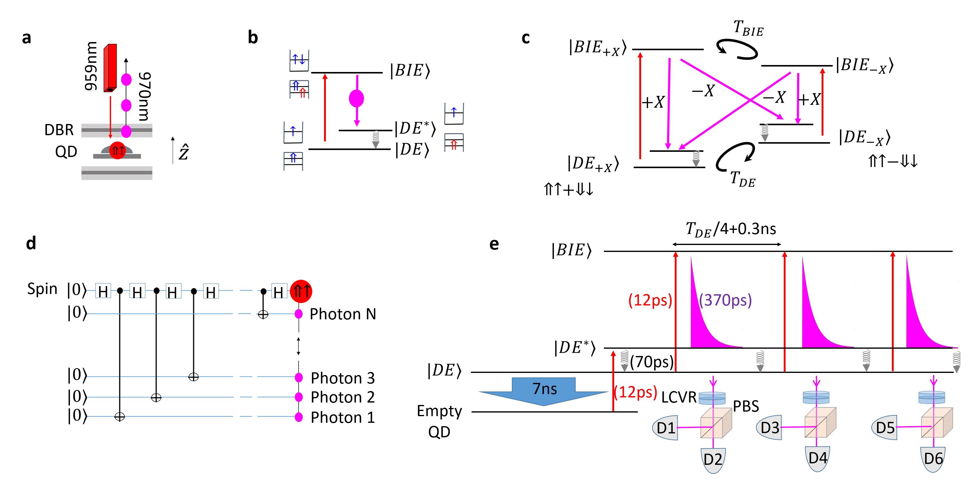
Figure 1: a) Schematic description of the QD-based device. DBR- distributed Bragg reflector. b) The energy levels of the DE - DE* - BIE system and the transitions between these levels. Each laser pulse (red upward arrow) excites the DE and photogenerates a BIE. The BIE then decays to an excited DE* by emitting a single-photon (downward pink arrow). The DE* then decays to its ground level by emitting acoustical phonon (curly downward arrow). c) The BIE-DE*-DE energy levels and the polarization-selection-rules for the optical transitions. Here +X (-X) describes horizontally (vertically) rectilinearly polarized optical transition. The short-range electron-hole exchange interaction removes the degeneracy between both the DE and the BIE two eigenstates. A coherent superposition of the DE (BIE) eigenstates precesses with a period marked by $T_{DE}$ ($T_{BIE}$). d) The cluster state repeating protocol contaning Hadamard gates acting on the QD confined spin followed by a CNOT- two qubit gates, which entangles the spin polarization with the polarization of an emitted photons. e) The experimental setup, pulse sequence, photon emissions, and detection for realizing and characterizing the cluster state. Blue downward wide-arrow is an optical-depletion 7ns long pulse (Schmidgall et al., 2015), which depletes the QD from carriers. Upward arrows are 12 ps long $\pi$-area laser pulses, while the downward pink exponential decays represent the emitted photons. We project the photons’ polarization using liquid-crystal-variable-retarders (LCVRs) and polarizing-beam-splitters (PBS) while looking for three consecutive photon detections.

II Cluster-state Generation - Method

In the heart of our device is a semiconductor QD. The QD contains a confined electronic-spin, which serves as the entangler qubit (Loss and DiVincenzo, 1998; DiVincenzo, 2000; Lindner and Rudolph, 2009). We define the sample growth direction, which is also the QD’s shortest dimension (about 3nm) as the quantization z-axis. The QD is embedded in a planar microcavity, formed by 2 Bragg-reflecting mirrors (Fig. 1a), facilitating efficient light-harvesting by an objective placed above the QD.

The DE is an electron-hole pair with parallel spins (Poem et al., 2010; Schwartz et al., 2015a, b), having two total angular momentum states of $\pm 2$ as projected on the QD z-axis. Since the DE optical activity is weak (Zieliński, Don, and Gershoni, 2015), it has long life and coherence time (Schwartz et al., 2015a; Cogan et al., 2018). Upon optical excitation, the DE ($\left|\Uparrow\uparrow\right\rangle$) is excited to form a biexciton (BIE) ($\left|\Uparrow\Uparrow\uparrow\downarrow\right\rangle$). The BIE is formed by pair of electrons in their first conduction-subband level and 2 heavy holes with parallel spins one in the first and one in the second valence-subband levels. Fig. 1b and Fig. 1c schematically describe the DE-BIE energy level structure, and the selection rules for optical transitions between these levels, respectively (Bayer et al., 2002; Ivchenko, 2005; Poem et al., 2010).

Each laser pulse (in red) excites the QD confined DE to its corresponding BIE state. The BIE decays to the DE* level within about 370ps by radiative recombination in which a single photon is emitted (marked in pink). The DE* then decays to the ground DE state by about 70ps spin-preserving acoustical-phonon relaxation. The energy difference between the emitted photon and the exciting laser allows us to spectrally filter the emitted single photons.

The eigenstates of the DE and BIE are given by: $\left|\pm X_{DE}\right\rangle=\left(\left|+Z_{DE}\right\rangle\pm\left|-Z_{DE}\right\rangle\right)/\sqrt{2}$ and $\left|\pm X_{BIE}\right\rangle=\left(\left|+Z_{BIE}\right\rangle\pm\left|-Z_{BIE}\right\rangle\right)/\sqrt{2}$. The energy differences between these eigenstates are about $1\mu eV$, smaller than the radiative width of the BIE optical transition ($\simeq 3\mu eV$) and much smaller than the spectral width of our laser pulse ($\simeq 100\mu eV$). It follows that a coherent superposition of the DE (BIE) eigenstates precesses with a period $T_{DE}=3.1ns$ ($T_{BIE}=5.6ns$), an order of magnitude longer than the BIE radiative time.

The DE and BIE act as spin qubits. Angular momentum conservation during the optical transitions between these two qubits imply the following $\pi$-system selection rules (Cogan et al., 2018):

$$\left|\Uparrow\uparrow\right\rangle \stackrel{{\scriptstyle\left|+Z\right\rangle}}{{\longleftrightarrow}}\left|\Uparrow\Uparrow\downarrow\uparrow\right\rangle,$$

$$\left|\Downarrow\downarrow\right\rangle \stackrel{{\scriptstyle\left|-Z\right\rangle}}{{\longleftrightarrow}}\left|\Downarrow\Downarrow\uparrow\downarrow\right\rangle.$$ (1)

where $\left|+Z\right\rangle$ ($\left|-Z\right\rangle$) is a right (left) -hand circularly polarized photon propagating along the +Z-direction. It thereby follows that a laser pulse polarized $\left|+X\right\rangle=\left(\left|+Z\right\rangle+\left|-Z\right\rangle\right)/\sqrt{2}$ coherently excites a superposition $\alpha\left|\Uparrow\uparrow\right\rangle+\beta\left|\Downarrow\downarrow\right\rangle$ of the DE spin qubit states to a similar superposition $\alpha\left|\Uparrow\Uparrow\uparrow\downarrow\right\rangle+\beta\left|\Downarrow\Downarrow\uparrow\downarrow\right\rangle$ of the BIE states. The BIE then radiatively decays into an entangled spin-photon state $\alpha\left|\Uparrow\uparrow\right\rangle\left|+Z\right\rangle+\beta\left|\Downarrow\downarrow\right\rangle\left|-Z\right\rangle$. Therefore the excitation and photon emission act as a 2-qubit entangling (CNOT) gate between the spin and the photon.

The method for generating the cluster state is described in Fig. 1d. The confined DE is resonantly excited repeatedly by a laser pulse to its corresponding BIE. The BIE decays radiatively by emitting a photon. The excitation and photon emission act as a two-qubit CNOT gate which entangles the emitted photon polarization qubit and the spin qubit, thus adding a photon to the growing photonic cluster. The excitation pulses are timed such that between the pulses the DE-spin precesses quarter of its precession period. This temporal precession can be ideally described as a unitary Hadamard gate acting on the spin qubit only. The combination of the CNOT 2-qubit gate and the Hadamard 1-qubit gate forms the basic cycle of the protocol which when repeated periodically generates the entangled spin + photons cluster state (Lindner and Rudolph, 2009).

For the experimental realization of the cluster protocol and the characterization of the generated state, we use the experimental setup described in Fig. 1e. The QD is first optically-emptied from carriers, making it ready for initialization. The first 7-ns-long optical pulse (Blue downward arrow) depletes the QD from charges and the remaining DE (Schmidgall et al., 2015). We then write the DE spin state using horizontally polarized 12-ps optical $\pi$-pulse to the DE* state. This is possible due to small mixing between the bright exciton (BE) and the DE (Schwartz et al., 2015b). The pulsed polarization defines the DE* initial spin state. The DE* then relaxes to its ground DE state, making the QD ready for implementing the cluster protocol. A sequence of resonantly tuned linearly polarized $\pi$-area laser pulses is then applied to the QD. Each pulse results in the emission of a photon from the QD’s BIE-DE optical transition. During the last emission, the BIE spin evolution can be conveniently used as a resource for the DE spin tomography (Cogan et al., 2020).

To characterize the generated multi-qubit quantum state, we project the polarization of the detected photons on 6 different polarization states using liquid-crystal-variable-retarders (LCVRs) and polarizing-beam-splitters (PBSs). We then use highly efficient transmission gratings to spectrally filter the emitted photons from the laser light. The photons are eventually detected by 6 efficient (>80%) fast single-photon superconducting detectors with temporal resolution of about 30ps.

III Cluster-state characterization

The cluster state entanglement robustness is characterized using three cycles of the repeated protocol. The characterization is done by correlating one, two, and three detected photon events. In all cases the last detected photon is used for the tomography of the DE-spin. We use two different orthogonal, +X and +Y linearly polarized excitation pulses respectively (Cogan et al., 2020). The +X-polarized laser pulse promotes the DE state to a similar superposition of BIE states, while +Y excitation introduces a $\pi/2$ phase shift to the superposition (Cogan et al., 2020). In addition, we utilize the BIE state evolution during its radiative decay back to the DE* to measure the degree-of-circular-polarization ($D_{cp}$) of the emission as a function of time:

$$D_{cp}(t)=\frac{P_{+Z}(t)-P_{-Z}(t)}{P_{+Z}(t)+P_{-Z}(t)},$$ (2)

where $P_{j}$ represents the detected photon polarization-projection on the j basis. By fitting the measured $D_{cp}(t)$ to a central-spin-evolution-model that we recently developed for QD confined charge carriers (Cogan et al., 2020), we accurately extract the DE spin state in the time of its excitation.

As we implement the protocol, we perform full tomographic measurements of the growing quantum state. First, we measure the initialized DE state. Then we apply one cycle of the protocol and measure the resulting spin+1photon state. Finally, we apply a second cycle of the protocol and measure the spin+2photons state.

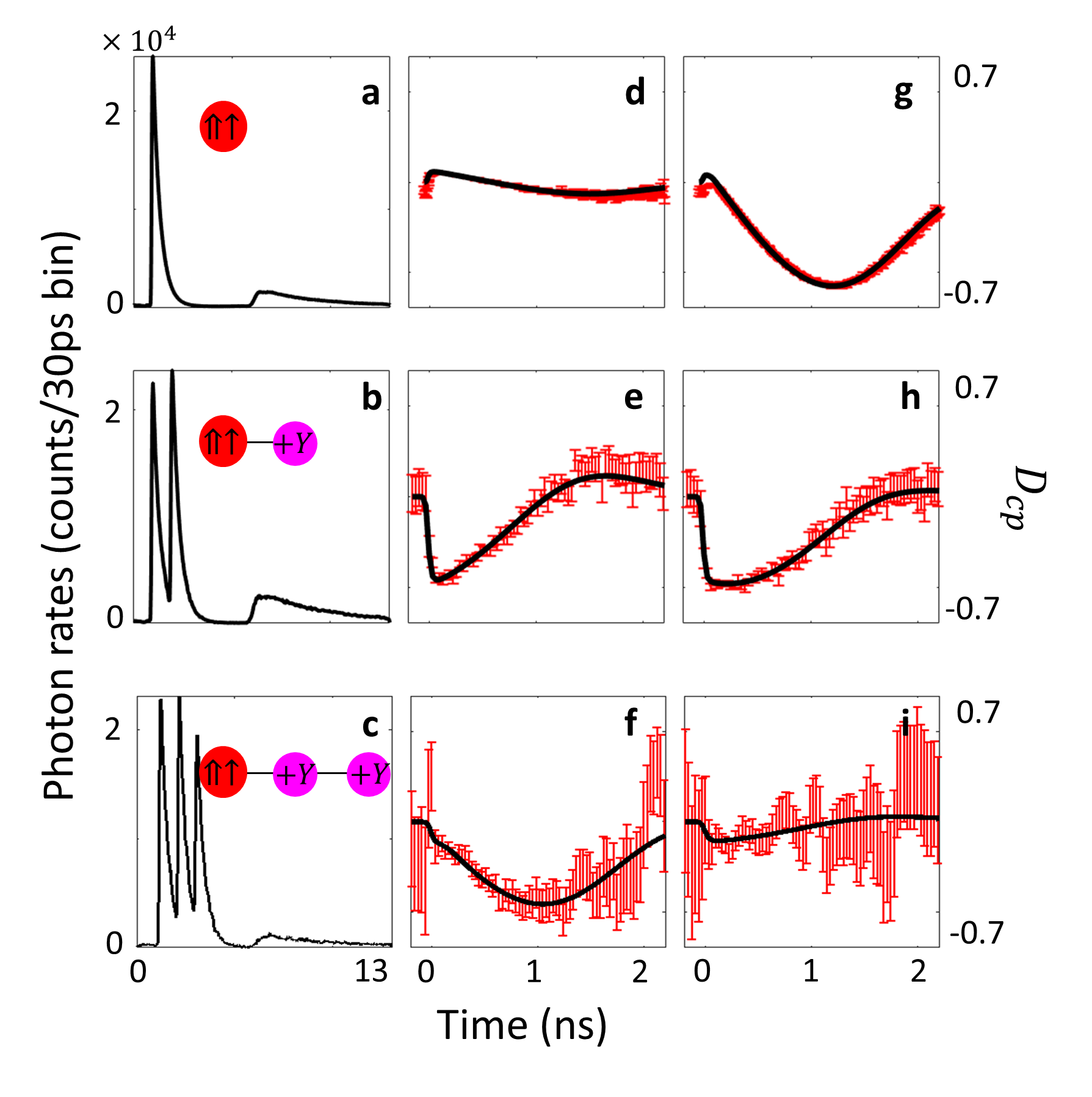
Figure 2: Example of one-, two-, and three-photon correlation measurements performed in characterizing the photonic cluster state. a), b), and c) are time resolved PL measurements of the BIE-DE optical transition following one-, two- ,and three-pulse excitations, respectively. d), e), and f) are time resolved degree of circular polarization measurements $D_{cp}(t)=\frac{P_{+Z}(t)-P_{-Z}(t)}{P_{+Z}(t)+P_{-Z}(t)}$ of the last detected photon, using horizontally polarized (+X) excitation pulse. g), h), and i) are the same as g), e), and f), using diagonally linearly polarized excitation pulse (+Y). The red data points describe the measured data and the solid black line describe the fitted model calculations (see Appendix). From the fitted model we extract the spin, spin+1 photon, and spin+2 photon density matrices elements.

In Fig 2 we present a small set of the measurements used to deduce the spin, spin+1photon, spin+2photon quantum states and the process map of the periodic cycle of the cluster protocol. The first row shows $D_{cp}$ measurements characterizing the initialized spin, the second row shows the $D_{cp}$ of the correlated spin+1photon state after the photon was projected on a +Y polarization basis, and the third row shows the $D_{cp}$ of the correlated spin+2photons state after both photons were projected on +Y polarization basis. Each row differs from the row above it by applying one additional cycle of the protocol. In all measurements shown in the Fig. 2, the DE was initialized to -X state. In each row, the left-panel displays time resolved PL, the center-panel (right-panel) displays time resolved $D_{cp}$ measured after +X (+Y) polarized excitation of the final spin. By fitting the $D_{cp}$ correlation measurements, we extract the following spin, spin+1photon, and spin+2photon polarization density matrix elements, respectively:

$$[S_{X},S_{Y},S_{Z}]=[-0.73,0.05,0.06]$$

$$[P_{Y}^{(1)}S_{X},P_{Y}^{(1)}S_{Y},P_{Y}^{(1)}S_{Z}]=[0.01,0.16,-0.59]$$

$$[P_{Y}^{(1)}P_{Y}^{(2)}S_{X},P_{Y}^{(1)}P_{Y}^{(2)}S_{Y},P_{Y}^{(1)}P_{Y}^{(2)}S_{Z}]=[0.03,-0.49,-0.08],$$

where $P_{j}^{(i)}$represents the polarization projection of the i’th-photon in the string, on the j polarization base, and $S_{j}$ is the DE-spin polarization, projected on the j base. The typical measurement uncertainties are about 0.01, 0.02, and 0.04 for the spin, spin+1photon, and spin+2photon polarization density matrix elements, respectively.

For a perfect initialization and application of the process we expect these polarization elements to be [-1,0,0], [0,0,-1], [0,-1,0] respectively. Here, the DE spin is initialized to the $-X$ state with polarization degree of 0.73, due to the limited efficiency of the depleting pulse (Schmidgall et al., 2015). After each cycle of the protocol, the measured $D_{cp}(t)$ is reduced by approximately 20%, indicating an exponential decay as expected (Popp et al., 2005; Schwartz et al., 2016).

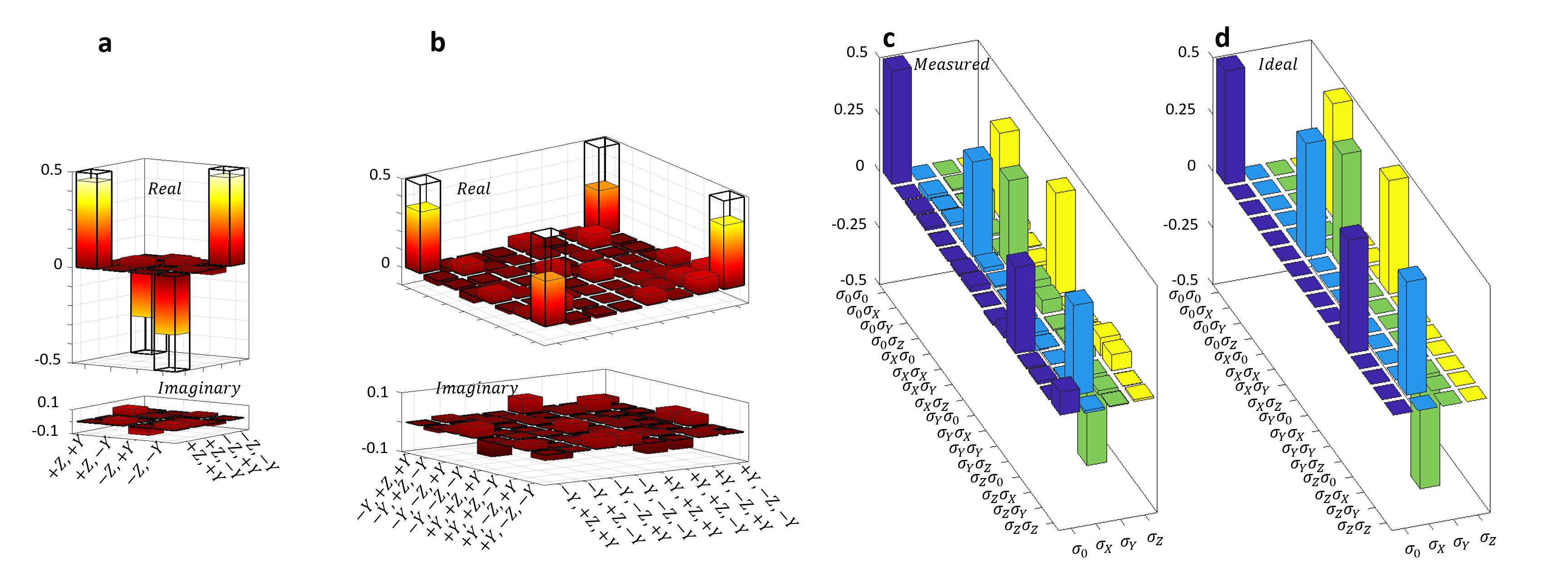
Figure 3: a) The measured DE+1photon density matrix. b) The measured DE+2photons density matrix. In a) and b), the colored bars represent measured density matrix elements, while the empty bars represent the ideal maximally entangled 2- and 3-qubit states. The fidelity of the measured density matrix to the ideal one is $F=0.77\pm 0.04$ in a) and $F=0.68\pm 0.07$ in b). In both cases, the DE spin is initialized to the $\left|-X_{DE}\right\rangle$ state with measured fidelity of $F=0.86\pm 0.02$ and then applying once or twice the process. The process map $\Phi$, which describes the system’s evolution in each cycle of the protocol is given by $\Phi(\hat{\rho}_{DE})=\underset{\alpha,\beta,\gamma}{\sum}\Phi_{\alpha\beta}^{\gamma}\rho_{\gamma}^{DE}\hat{\sigma}_{\alpha}\hat{\sigma}_{\beta}$, where $\hat{\rho}_{DE}=\underset{\gamma}{\sum}\rho_{\gamma}^{DE}\hat{\sigma}_{\gamma}$ is the density matrix that describes the input DE state and $\Phi(\hat{\rho}_{DE})$ describes the DE+1photon state after applying the process on the input DE qubit. Here, $\alpha,\,\beta,$ and $\gamma$ run over $O,\,X,\,Y$, and $Z$, where $\hat{\sigma}_{0}$ is the identity matrix and $\hat{\sigma}_{X}$, $\hat{\sigma}_{Y}$, and $\hat{\sigma}_{Z}$ are the corresponding Pauli matrices. The 64 real parameters $\Phi_{\alpha\beta}^{\gamma}$ , thus fully specify $\Phi$. c) The process map $\Phi_{\alpha\beta}^{\gamma}$ as measured by the quantum process tomography. The matrix elements of $\Phi_{\alpha\beta}^{\gamma}$ are presented such that the rows correspond to the indices $\alpha\beta$ of the DE+1photon output state, and the columns correspond to the index $\gamma$ of the input DE state. d) The process map $\Phi_{\alpha\beta}^{\gamma}$, calculated assuming the ideal protocol (CNOT and Hadamard gates), as in Fig. 1d.

The measured correlations are used to infer directly the spin+1photon 2qubit state, obtained by applying one cycle of the protocol, the spin+2photon state obtained by applying two cycles of the protocol, and a full process tomography of the periodic cycle of the cluster protocol.

To measure the spin+1photon density matrix (displayed in Fig. 3a), we use a set of 12 DE-photon $D_{cp}(t)$ correlation measurements. Two of those measurements are displayed in Fig. 2e and Fig. 2h. The measured density matrix has fidelity of $F=0.77\pm 0.04$ with the maximally entangled Bell state. To measure the spin+2photons 3-qubit density matrix (displayed in Fig. 3b) we use a set of 72 $D_{cp}(t)$ DE-2photon correlation measurements. Two of those measurements are displayed in Fig. 2f and 2i. The measured spin+2photons density matrix has fidelity of $0.68\pm 0.07$ with the maximally entangled 3-qubit state.

We produce the cluster state by repeatedly applying the same process, as shown in the protocol of Fig. 1d. As a result, one can fully characterize the cluster state for any number of qubits if the single-cycle process-map is known (Schwartz et al., 2016). Ideally, the process-map contains a CNOT and a Hadamard gate. It maps the 2$\times$2 spin qubit density matrix into a 4$\times$4 density matrix representing the entangled spin-photon state. The process map $\Phi$ can be fully described by a 4$\times$16 positive and trace-preserving map with 64 real matrix elements.

We use the convention $\Phi(\hat{\rho}_{DE})=\underset{\alpha,\beta,\gamma}{\sum}\Phi_{\alpha\beta}^{\gamma}\rho_{\gamma}^{DE}\hat{\sigma}_{\alpha}\hat{\sigma}_{\beta}$ , where $\hat{\rho}_{DE}=\underset{\gamma}{\sum}\rho_{\gamma}^{DE}\hat{\sigma}_{\gamma}$ is the density matrix that describes the input DE state and $\Phi(\hat{\rho}_{DE})$ describes the DE+1photon state after one application of the process to the input DE state. The sums are taken over $\alpha,\beta,\gamma=O,X,Y,Z$, where $\hat{\sigma}_{0}$ is the identity matrix and $\hat{\sigma}_{X}$,$\hat{\sigma}_{Y}$,$\hat{\sigma}_{Z}$ are the corresponding Pauli matrices. The 64 real parameters $\Phi_{\alpha\beta}^{\gamma}$ thus fully specify $\Phi$.

Fig. 3c shows the results of the full-tomographic measurements of the process map. For acquiring these measurements, we initialize the DE-spin-state to six different states from three orthogonal bases (Schwartz et al., 2015b). For each of those 6 states we use 2 $D_{cp}(t)$ single-photon measurements like the measurements displayed in Fig. 2d and Fig. 2g for tomography. Then we apply one cycle of the protocol for each initialization and measure the resulting spin+1photon states by projecting the first photon on different orthogonal polarization bases (James et al., 2001) and correlating it with the $D_{cp}(t)$ of the second photon. For characterizing each of those 6 spin+1photon states, we use 12 $D_{cp}(t)$ 2-photon correlations measurements like the ones presented in Fig. 2e and Fig. 2h.

To obtain the physical process map that best fits our measured results, we use a specifically developed edge-sensitive twisted-gradient-descent minimization method (See Appendix). It is well known that the space of physical completely-positive (CP) maps can be identified with a cone-like-space where any unitary process sits on an extremal ray of the cone. To find the best CP fit of $\Phi$ therefore requires minimizing a known function $F$ (representing minus log likelihood) over this cone. Gradient descent tries to find the minimum of a function $F(x)$ by going roughly along gradient lines of $F$. Our newly developed approach uses an edge-sensitive twisted-gradient-descent in order to prevent our gradient descent solution from getting stuck in the boundary of the physically allowed cone-like region.

Fig. 3c-d presents the physical CP-process-map obtained using this method. We compare the acquired physical process with the ideal unitary process of the cluster protocol. The fidelity (Jozsa, 1994; Schwartz et al., 2016) between the two processes is 0.83. The obtained fidelity is higher than in the previous demonstration (Schwartz et al., 2016). The higher fidelity is attributed to the 3-fold shorter time between the excitations, which reduces the influence of the DE decoherence during its precession. The relatively high fidelity to the ideal protocol indicates that our device can deterministically generate photonic cluster states of high quality, thereby providing a better resource for quantum information processing.

IV Discussion

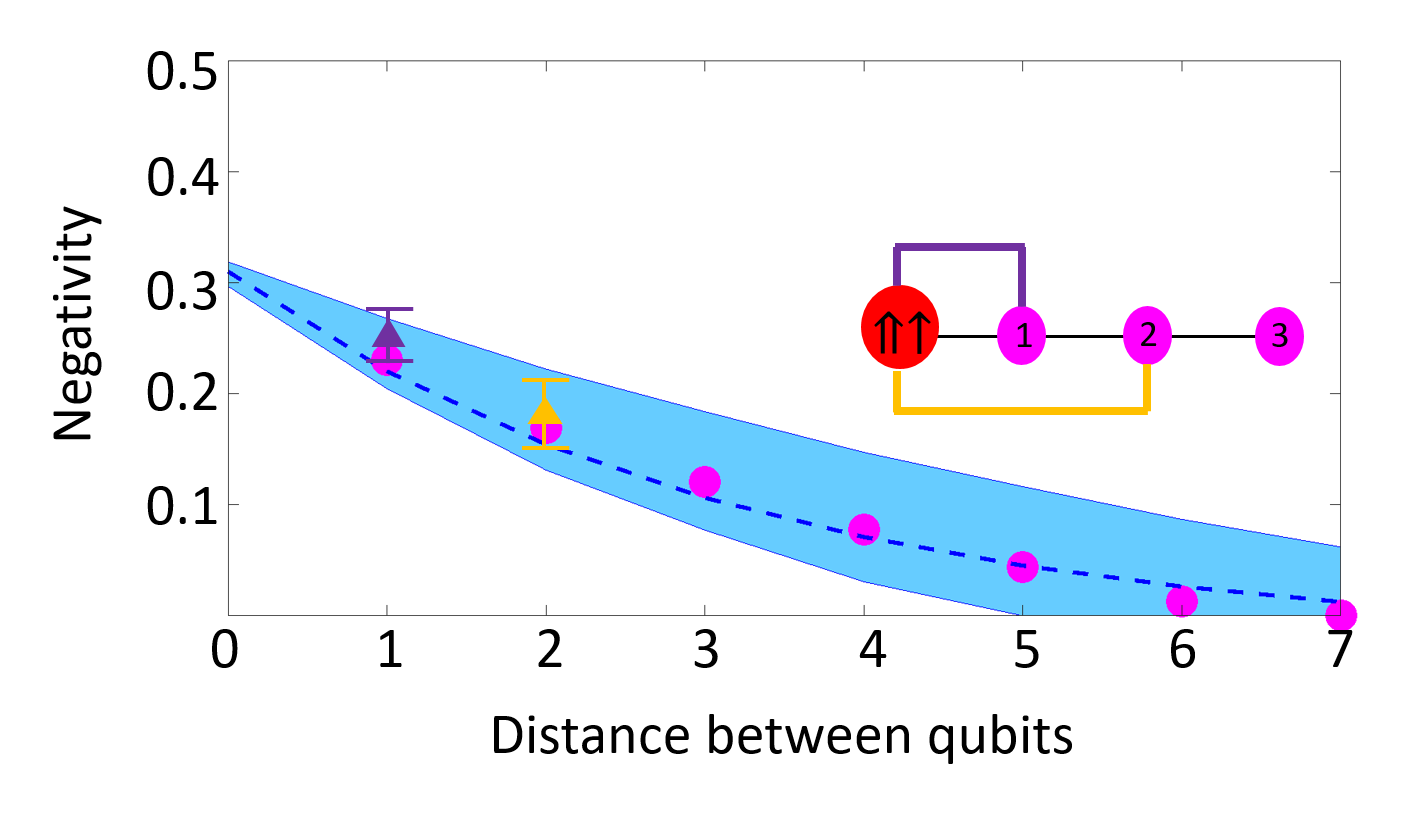
Figure 4: The localizable entanglement (LE - pink circles) in the generated state vs. the distance between two qubits in the string. The pink circles correspond to the LE between qubits m and m + d in the state of DE+Nphotons obtained using the measured process map. The dashed lines represent the best fit to an exponential decay law $N(d)=N_{nn}\exp\left(-(d-1)/\zeta_{LE}\right)$, where $N_{nn}$ is the negativity (Peres, 1996) between nearest-neighbor qubits, d is the distance between the qubits, and $\zeta_{LE}$ is the characteristic decay-length of the LE. The light-blue shaded area represents one standard deviation of the uncertainty in the measurements determining the process map. The purple and yellow data points represent the directly measured LE of the DE and the first emitted photon in a two- and a three-qubit string, respectively, acquired from the complete tomographic measurements of those states presented in Fig. 3c and d.

We characterize the robustness of the entanglement in the 1D cluster-state using the notion of localizable entanglement (LE) (Verstraete, Popp, and Cirac, 2004). The LE is the negativity (Peres, 1996) between two qubits in the cluster after all the other qubits are projected onto a suitable polarization-basis. The LE decays exponentially with the distance between the qubits (Popp et al., 2005; Schwartz et al., 2016):

$$N(d)=N_{nn}\exp\left(-(d-1)/\zeta_{LE}\right),$$ (3)

where $N_{nn}$ is the negativity between nearest-neighbor qubits, d is the distance between the qubits, and $\zeta_{LE}$ is the characteristic decay-length of the LE. In Fig. 4, we plot using pink circles the LE in the state of a spin+Nphotons, obtained from the measured process map, as a function of the distance between two qubits in the string. As expected, the LE in the 1D cluster state decays exponentially with the distance between the two qubits (Popp et al., 2005). Fig. 4 shows that the entanglement in the cluster persists up to up to six photons. This presents an improvement over Ref. (Schwartz et al., 2016), resulting from the reduction in the DE spin decoherence between the optical pulses.

The negativity between nearest neighbor and next nearest neighbor 2 qubits can be directly obtained from our quantum state tomography. The entanglement between the DE and the photon emitted after one cycle of the protocol is obtained from the density matrix of the DE+1photon in Fig. 3a which has negativity of $N=0.27\pm 0.03$. This negativity is marked as a purple data point in Fig. 4. Similarly, the spin+2photons 3-qubit state resulted from application of two cycles of the protocol is represented by the 3-qubit density matrix, displayed in Fig. 3b. The negativity of the density matrix of the two external qubits, after projecting the central qubit on the X polarization basis is $N=0.18\pm 0.05$, marked by the yellow point in Fig. 4.

In summary, we demonstrate a gigahertz-rate deterministic generation of entangled photons in a cluster state, which is 3-times faster than previously demonstrated. We developed a novel method for spin - multi photon quantum state tomography and for characterizing the periodic process map which generates the photonic cluster state. Using this method we show that the enhanced cluster generation rate also improves the robustness of the entanglement in the generated multi -photon state. The measured process map has fidelity of 0.83 to the ideal one, and the entanglement in the cluster state persists up to 6 consecutive qubits. Our studies combined with further feasible optimizations of the device may lead to implementations of quantum communication and efficient distribution of quantum entanglement between remote nodes.

Appendix A the process likelihood function

The basic (single cycle) process taking the QD-spin into a spin plus emitted photon is described by a process map $\Phi$ taking one-qubit state into a two-qubit state. Expanding these quantum states in terms of Pauli matrices allows writing the map as

$$\rho=\sum r_{\mu}\sigma^{\mu}\mapsto\Phi(\rho)=\sum r_{\mu}\phi_{\nu\lambda}^{\mu}\sigma^{\nu}\otimes\sigma^{\lambda}.$$

Here $\phi_{\nu\lambda}^{\mu}$ with $\mu\nu\lambda\in\{0,x,y,z\}$ are 64 real coefficient which define the process map $\Phi$.

The trace preserving condition $Tr\Phi(\rho)=Tr\rho\forall\rho$ fixes 4 out of the 64 coefficient $\phi_{\nu\lambda}^{\mu}$ namely it requires that $\phi_{00}^{\mu}=\frac{1}{2}\delta_{\mu 0}$. We wish to estimate the other 60 parameter by finding the best fit to the experimental data.

In an experiment where the initial spin was $\vec{s}$ and the emitted photon was projected on state of spin $\vec{p}$ we would ideally expect the measured rate $R$ of photon emission and final spin $\vec{S}$ to satisfy $\phi_{\nu\lambda\mu}s_{\mu}p_{\lambda}=R\;S_{\nu}$. Here $s,p,S$ are four-vectors whose zeroth component equals 1 and their spatial components are $\vec{s},\vec{p},\vec{S}$. Repeating such measurement for six different spin polarizations $\vec{s}$ and six different photon polarizations $\vec{p}$ gives $6\times 6\times 4=144$ equations for the $60$ unknown components of $\Phi$.

A straightforward approach to determine $\Phi$ is then to use a least square method minimizing the expression $F_{0}=\sum_{p,s,\nu}\frac{1}{\Delta_{ps\nu}^{2}}\left[\phi_{\nu\lambda\mu}s_{\mu}p_{\lambda}-R\;S_{\nu}\right]^{2}.$ (Essentially representing minus log likelihood.) Here $\Delta_{ps\nu}$ are the error estimates of the corresponding measurement. A slightly more sophisticated approach would recall that appearance of each of the six initial polarizations $\vec{s}$ in 24 different sums, can potentially make the errors correlated. One way to take this into consideration is to use a more complicated square sum constructed using a non-diagonal covariance matrix. A completely equivalent method consists of defining new variables $\vec{s^{\prime}}$ representing the ’true’ initial polarization of the DE and using the new sum of square error function $\tilde{F}_{0}=\tilde{F}_{0}(\phi,s^{\prime})$ defined by

$$\tilde{F}_{0}(\phi,s^{\prime})=\sum_{p,s,\nu}\frac{1}{\Delta_{ps\nu}^{2}}\left[\phi_{\nu\lambda\mu}s^{\prime}_{\mu}p_{\lambda}-R\;S_{\nu}\right]^{2}+\sum_{s}\sum_{i=1}^{3}\left(\frac{s^{\prime}_{i}-s_{i}}{\Delta s_{i}}\right)^{2}$$

Minimizing this expression with respect to $s^{\prime}$ yields a standard square sum $F_{0}(\phi)$ corresponding to the correct non-diagonal covariance matrix. We looked for a minimum of $\tilde{F}_{0}(\phi,s^{\prime})$ with respect to both the process map $\phi$ and the unknown initialization polarizations $s^{\prime}$.

Appendix B Completely positive condition and twisted gradient descent.

It is well known that to be physically acceptable, a process map $\Phi$ must be completely positive (CP). A process map is CP iff the associated Choi matrix which may be defined (up to unimportant normalization factor) by

$$C_{\Phi}=\sum\phi_{\nu\lambda}^{\mu}\;\overline{\sigma_{\mu}}\otimes\sigma^{\nu}\otimes\sigma^{\lambda}$$ (4)

is positive (semi-definite) $C_{\Phi}\geq 0$. The bar over $\sigma_{\mu}$ denotes complex conjugation and we make no distinction here between lower and upper indices. In general the Choi matrix $C_{\Phi}$ is a (complex) hermitian $8\times 8$ matrix which may be used as an alternative description of $\Phi$.

Simple minded naive minimization of $F_{0}$ leads to a process map which is not CP and hence not physically acceptable. To understand why this happens, recall that our process is very close to an idealized process which is unitary. Any unitary process is an extreme point of the cone of CP-maps and has a rank-1 Choi matrix. In other words, for a unitary process 7 out of the 8 eigenvalues of the Choi matrix vanish. Our $\Phi$ being close to unitary has therefore 7 very small Choi matrix eigenvalues. It is thus not surprising that very small experimental errors can lead us to estimate some of these eigenvalues as negative, in contradiction with the CP condition. (Had our $\Phi$ been equal to the ideal unitary map, a small random error in each eigenvalue would lead to non CP map with probability $\frac{127}{128}=0.992$) In other words, the encountered difficulty is actually a good sign indicating that our process has quite low decoherence.

To find the best CP fit of $\Phi$ therefore requires minimizing a known function $F$ (representing minus log likelihood) over the subset of CP-maps, which as explained above may be identified (through the Choi representation) with the cone of positive matrices. This is closely related to the extensively studied field of convex optimization. We have not found however in the convex optimization literature a method which looks to exactly fit our problem. We have therefore devised a method of our own (explained below) which is a variant of the well known gradient descent.

Gradient descent tries to find the minimum of a function $F(x)$ by going roughly along gradient lines of $F$. It corresponds to (numerically discretized) solution to the equation $\frac{d}{dt}x^{i}=-g^{ij}\partial_{j}F(x)$. The (inverse) metric tensor $g^{ij}$ is often taken to be the standard euclidean metric $\delta_{ij}$. Such choice is not mandatory and in fact one may choose any (positive) metric. We suggest to use a smarter choice of the metric in order to prevent our gradient descent solution from getting stuck in the boundary of the physically allowed region.

It is easiest to understand our approach by considering minimization over a simple region like $\{(x,y)\in\mathbb{R}^{2}\mid x,y\geq 0\}$. In this case our approach to minimizing $F(x,y)$ would correspond to using iteration steps with $(\Delta x,\Delta y)\propto(x\partial_{x}F,y\partial_{y}F)$. Assuming that both derivatives of $F$ are $O(1)$, one sees that if our approximate estimate $(x,y)$ of the minimizer is very close to one of the boundaries e.g. if it has $x\ll 1$ and $y=O(1)$ then the next step $(\Delta x,\Delta y)$ would adapt to this fact by being almost parallel to the $y$-axis. One can then go a long $\sim O(1)$ distance along this direction without crossing the boundary. This is in contrast to hitting the boundary after a distance $O(x)\ll 1$ which would result from using the standard metric $g_{ij}=\delta_{ij}$.

Since the CP - condition is easier to formulate in terms of Choi matrices, let us consider the (square sum) function we want to minimize as a function $F(A)$ over the (real vector space) of hermitian matrices . The standard euclidean gradient of $F$ may be identified with the matrix $\nabla F$ whose elements are $(\nabla F)_{ij}=\frac{\partial F}{\partial a_{ji}}$. (This relation may be a bit confusing since the elements $a_{ij}$ of $A$ are complex.) An equivalent and possibly more rigorous definition starts by expressing $A$ as $A=\sum a_{\alpha}\Xi_{\alpha}$ where $a_{\alpha}\in\mathbb{R}$ and $\{\Xi_{\alpha}\}$ are some basis for the space of Hermitian matrices which is orthonormal in the sense $Tr(\Xi_{\alpha}\Xi_{\beta})=N\delta_{\alpha\beta}$ with some normalization $N$. Note that our $A$ being a process Choi matrix, is already given to us in such a form by Eq.(4). One can then write $\nabla F=\sum\Xi_{\alpha}\partial_{\alpha}F$.

The gradient we use corresponds to a non-flat riemanian metric and may be expressed as $\tilde{\nabla}F=\sqrt{A}(\nabla F)\sqrt{A}$ (where $\nabla F$ is as above). We therefore look for a minimum of $F$ over the set of positive (semi-definite) matrices by using a gradient descent step of the form

$$A\mapsto A+\Delta A,\;\;\;\;\;\Delta A=-q\sqrt{A}(\nabla F)\sqrt{A}$$

Here $q>0$ is a scalar chosen so that $F(A+\Delta A)$ is minimal under the constraint $A+\Delta A\geq 0$ . Note that if $\nabla F=O(1)$ then the positivity constraint allows $q$ to remain $O(1)$ even if $A$ is very close to the boundary of the cone of positive matrices. All our process map estimations were obtained using this minimization scheme which we implemented using Mathematica^TM.

Although the basic method described above works reasonably well, we found that some extra improvement is gained if after each step we push $A$ slightly away from the boundary of the allowed region by updating it as $A\rightarrow(1-\varepsilon)A+\frac{1}{2}\varepsilon I$ with $\varepsilon\ll 1$. (We suspect that the need for this step might be related to the finite precision of the numerical calculations.) We increase or decrease $\varepsilon$ dynamically during the computation, depending on the performance of previous iteration step. In practice $\varepsilon$ ranged between $10^{-4}$ and $10^{-10}$ and scaled roughly as 2-3 times the minimal eigenvalue of $A$.

The modified gradient descent method described here is quite general and can be applied to any $F(A)$. In practice, our $F(A)$ was of the form $F(A)=F_{0}(A)+\sum_{\mu=0}^{3}\lambda_{\mu}Tr(A(\sigma_{\mu}\otimes I\otimes I))$ where $F_{0}(A)$ is the square sum described in subsection A, and the second term consists of 4 lagrange multipliers required to enforce the normalization condition $\phi_{00}^{\mu}=\frac{1}{2}\delta_{\mu 0}$. The values of the multipliers $\lambda_{\mu}$ at each iteration step are easily determined numerically by requiring that $\Delta A=-q\sqrt{A}(\nabla F)\sqrt{A}$ does not break the normalization condition. This amount to demanding the partial trace $Tr_{2,3}(\sqrt{A}(\nabla F)\sqrt{A})$ to vanish, which is just a linear set of equations for $\lambda_{\mu}$.

References

- Raussendorf and Briegel (2001) R. Raussendorf and H. J. Briegel, Physical Review Letters 86, 5188 (2001).
- Raussendorf, Browne, and Briegel (2003) R. Raussendorf, D. E. Browne, and H. J. Briegel, Physical Review A 68 (2003), 10.1103/physreva.68.022312.
- Briegel et al. (2009) H. J. Briegel, D. E. Browne, W. Dür, R. Raussendorf, and M. V. den Nest, Nature Physics 5, 19 (2009).
- Briegel et al. (1998) H.-J. Briegel, W. Dür, J. I. Cirac, and P. Zoller, Physical Review Letters 81, 5932 (1998).
- Zwerger, Dür, and Briegel (2012) M. Zwerger, W. Dür, and H. J. Briegel, Physical Review A 85 (2012), 10.1103/physreva.85.062326.
- Zwerger, Briegel, and Dür (2013) M. Zwerger, H. J. Briegel, and W. Dür, Physical Review Letters 110 (2013), 10.1103/physrevlett.110.260503.
- Azuma, Tamaki, and Lo (2015) K. Azuma, K. Tamaki, and H.-K. Lo, Nature Communications 6 (2015), 10.1038/ncomms7787.
- Briegel and Raussendorf (2001) H. J. Briegel and R. Raussendorf, Physical Review Letters 86, 910 (2001).
- Hein, Eisert, and Briegel (2004) M. Hein, J. Eisert, and H. J. Briegel, Physical Review A 69 (2004), 10.1103/physreva.69.062311.
- Walther et al. (2005) P. Walther, K. J. Resch, T. Rudolph, E. Schenck, H. Weinfurter, V. Vedral, M. Aspelmeyer, and A. Zeilinger, Nature 434, 169 (2005).
- Prevedel et al. (2007) R. Prevedel, P. Walther, F. Tiefenbacher, P. Böhi, R. Kaltenbaek, T. Jennewein, and A. Zeilinger, Nature 445, 65 (2007).
- Lu et al. (2007) C.-Y. Lu, X.-Q. Zhou, O. Gühne, W.-B. Gao, J. Zhang, Z.-S. Yuan, A. Goebel, T. Yang, and J.-W. Pan, Nature Physics 3, 91 (2007).
- Tokunaga et al. (2008) Y. Tokunaga, S. Kuwashiro, T. Yamamoto, M. Koashi, and N. Imoto, Physical Review Letters 100 (2008), 10.1103/PhysRevLett.100.210501.
- Kimble (2008) H. J. Kimble, Nature 453, 1023 (2008).
- Munro et al. (2012) W. J. Munro, A. M. Stephens, S. J. Devitt, K. A. Harrison, and K. Nemoto, Nature Photonics 6, 777 (2012).
- Lindner and Rudolph (2009) N. H. Lindner and T. Rudolph, Physical Review Letters 103, (2009).
- Schwartz et al. (2016) I. Schwartz, D. Cogan, E. R. Schmidgall, Y. Don, L. Gantz, O. Kenneth, N. H. Lindner, and D. Gershoni, Science 354, 434 (2016).
- James et al. (2001) D. F. V. James, P. G. Kwiat, W. J. Munro, and A. G. White, Physical Review A 64 (2001), 10.1103/physreva.64.052312.
- Gonçalves, Gomes-Ruggiero, and Lavor (2015) D. Gonçalves, M. Gomes-Ruggiero, and C. Lavor, Optimization Methods and Software 31, 328 (2015).
- Bolduc et al. (2017) E. Bolduc, G. C. Knee, E. M. Gauger, and J. Leach, npj Quantum Information 3 (2017), 10.1038/s41534-017-0043-1.
- Cogan et al. (2018) D. Cogan, O. Kenneth, N. H. Lindner, G. Peniakov, C. Hopfmann, D. Dalacu, P. J. Poole, P. Hawrylak, and D. Gershoni, Physical Review X 8 (2018), 10.1103/physrevx.8.041050.
- Schmidgall et al. (2015) E. R. Schmidgall, I. Schwartz, D. Cogan, L. Gantz, T. Heindel, S. Reitzenstein, and D. Gershoni, Applied Physics Letters 106, 193101 (2015).
- Loss and DiVincenzo (1998) D. Loss and D. P. DiVincenzo, Physical Review A 57, 120 (1998).
- DiVincenzo (2000) D. P. DiVincenzo, Fortschritte der Physik 48, 771 (2000).
- Poem et al. (2010) E. Poem, Y. Kodriano, C. Tradonsky, N. H. Lindner, B. D. Gerardot, P. M. Petroff, and D. Gershoni, Nature Physics 6, 993 (2010).
- Schwartz et al. (2015a) I. Schwartz, E. R. Schmidgall, L. Gantz, D. Cogan, E. Bordo, Y. Don, M. Zielinski, and D. Gershoni, Physical Review X 5, (2015a).
- Schwartz et al. (2015b) I. Schwartz, D. Cogan, E. R. Schmidgall, L. Gantz, Y. Don, M. Zieliński, and D. Gershoni, Physical Review B 92, (2015b).
- Zieliński, Don, and Gershoni (2015) M. Zieliński, Y. Don, and D. Gershoni, Physical Review B 91, (2015).
- Bayer et al. (2002) M. Bayer, G. Ortner, O. Stern, A. Kuther, A. A. Gorbunov, A. Forchel, P. Hawrylak, S. Fafard, K. Hinzer, T. L. Reinecke, S. N. Walck, J. P. Reithmaier, F. Klopf, and F. Schäfer, Physical Review B 65, (2002).
- Ivchenko (2005) E. L. Ivchenko, Optical Spectroscopy of Semiconductor Nanostructures (Alpha Science, 2005).
- Cogan et al. (2020) D. Cogan, G. Peniakov, Z.-E. Su, and D. Gershoni, Physical Review B 101 (2020), 10.1103/physrevb.101.035424.
- Popp et al. (2005) M. Popp, F. Verstraete, M. A. Martín-Delgado, and J. I. Cirac, Physical Review A 71 (2005), 10.1103/PhysRevA.71.042306.
- Jozsa (1994) R. Jozsa, Journal of Modern Optics 41, 2315 (1994).
- Peres (1996) A. Peres, Physical Review Letters 77, 1413 (1996).
- Verstraete, Popp, and Cirac (2004) F. Verstraete, M. Popp, and J. I. Cirac, Physical Review Letters 92 (2004), 10.1103/physrevlett.92.027901.
- Note (1) We identify H,B,R polarizations with respectively.
- Note (2) The error estimate appearing in is constructed in the standard way from the error estimates and . The error is now taken care of by the second term (and is negligible anyway).
- Note (3) It is convenient to extend to arbitrary matrices by defining .
- Note (4) Euclidean gradient descent fails even if one includes similar improvement in it.
- Note (5) The need for lagrange multiplier is a cost we pay for using non flat metric. In flat metric, the constraints may be solved trivially.