UniFaceGAN: A Unified Framework for Temporally Consistent Facial Video Editing
Abstract
Recent research has witnessed advances in facial image editing tasks including face swapping and face reenactment. However, these methods are confined to dealing with one specific task at a time. In addition, for video facial editing, previous methods either simply apply transformations frame by frame or utilize multiple frames in a concatenated or iterative fashion, which leads to noticeable visual flickers. In this paper, we propose a unified temporally consistent facial video editing framework termed UniFaceGAN. Based on a 3D reconstruction model and a simple yet efficient dynamic training sample selection mechanism, our framework is designed to handle face swapping and face reenactment simultaneously. To enforce the temporal consistency, a novel 3D temporal loss constraint is introduced based on the barycentric coordinate interpolation. Besides, we propose a region-aware conditional normalization layer to replace the traditional AdaIN or SPADE to synthesize more context-harmonious results. Compared with the state-of-the-art facial image editing methods, our framework generates video portraits that are more photo-realistic and temporally smooth. Our project is available at here.
Index Terms:
Facial video editing, dynamic training sample selection, 3D temporal loss, region-aware conditional normalization.I Introduction
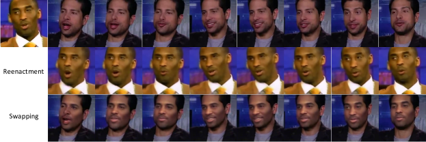
Facial video editing is an extensively studied task in the industry due to its widespread applications in movie composition, computer games, and privacy protection. It includes face swapping [1, 2, 3, 4, 5, 6], face reenactment [7, 8, 9, 10, 11, 12, 13, 14, 15], . Face swapping aims at replacing one person’s identity with another while keeping the original attributes unchanged, e.g. head pose, facial expression, background, etc. Face reenactment is another task that focuses on transferring the facial poses and expressions from the others.
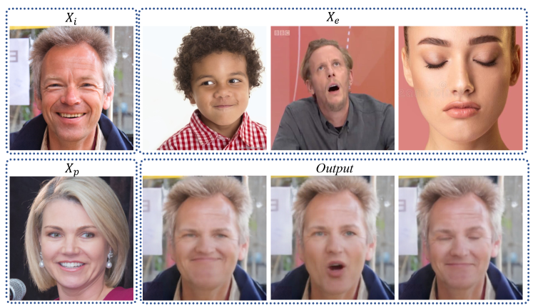
Most of the previous works have regarded face swapping and face reenactment as separate tasks and could only handle either of them. In this work, we devote ourselves to developing a more unified framework termed UniFaceGAN which settles face swapping and face reenactment jointly. Besides accomplishing the existing tasks, more surprisingly, our method also supports a novel application, which disentangles and remixes the facial characteristics from three different individuals. Specifically, we recombine the identity, expression, and appearance information extracted from three individual image frames to synthesize a photo-realistic video portrait. Notably, we name it “appearance" as it contains both the background and the pose information. We refer to this novel editing application as “fully disentangled manipulation" in our paper.
Despite tremendous advances in image facial editing, it is still challenging to perform video-level editing because of the temporal diversity. Simply applying transformations frame by frame inevitably induces temporal inconsistency, such as visual flickers. To address this issue, several methods have been developed. For face swapping, FSGAN [6] generates the output in an iterative way. However, reusing the previous frames recursively incurs error accumulation, which brings about more distortion. For face reenactment, [14, 11] regularize temporal relationships implicitly by concatenating multiple frames before feeding them to the networks. However, these methods lack explicit supervision. In this paper, we introduce a novel 3D temporal loss based on the dense optical flow map via the barycentric coordinate interpolation, which provides explicit supervision to guarantee the temporally consistent outputs.
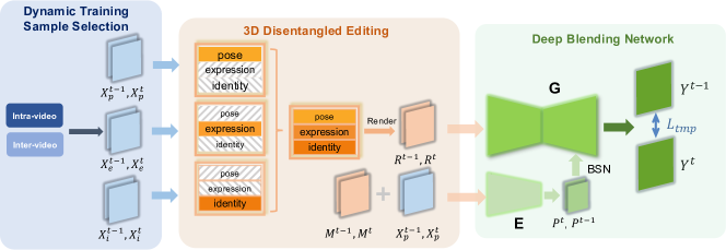
UniFaceGAN has three cascaded procedures, namely Dynamic Training Sample Selection, 3D Disentangled Editing, and Deep Blending Network. The Dynamic Training Sample Selection mechanism is designed to sample training data in both intra-video and inter-video manners, which facilitates our multi-task training. In the 3D Disentangled Editing stage, we incorporate a 3D Morphable Model (3DMM) [16, 17] reconstruction module to decompose a video portrait into pose, expression, and identity coefficients. Then we recombine these factors according to the specific task to get a transformed face sequence through a rasterization renderer. As for the Deep Blending Network, we feed the rendered transformed face and the auxiliary appearance hint to a Generative Adversarial Network, which translates the input to the photo-realistic result.
We’re not the first to introduce the 3D reconstruction technology into facial editing and the pioneering works [1, 18] also adopt a 3D-to-2D generation idea for accomplishing face reenactment for a single pre-determined person. However, our UniFaceGAN differs in the following two respects. Firstly, UniFaceGAN takes an additional appearance image as input and unifies the solutions of multiple video portrait manipulation tasks for arbitrary persons in a multi-task manner. Besides, the appearance image also serves as a background hint in the 3D Disentangled Editing stage, which settles the problem of blur background and generates more photo-realistic outputs. Introducing the 3D Disentangled Editing stage brings several advantages. First, compared to 2D-based methods [14, 19, 6, 20], explicitly reconstructing a 3D face can naturally collect that information in the 3D space. Besides, 3DMM has already decomposed pose, expression and identity information, which can be recombined to generate a novel desired 3D face. On the contrary, the pose and expression information in 2D facial landmarks cannot be decoupled, leading to the limited manipulation freedom. In addition, it is worth mentioning that sparse 2D landmarks lack facial texture details, thus suffering from blurry generation results. In contrast, rendering the 3DMM model with texture details provides more informative and realistic hints.
Since the facial information comes from the rendered face and the appearance image provides the background hint, Deep Blending Network uses two separate networks to tackle these two kinds of clues. Specifically, it consists of an encoder-decoder backbone and an appearance embedder, serving as the facial and non-facial feature extractors respectively. The encoder-decoder backbone takes a rendered 3D face as input, while the appearance embedder maps the concatenation of the appearance image and the non-facial area binary mask into a low-resolution feature map. Then, the facial and non-facial clues are fused through our proposed region-aware conditional normalization layer (RCN) which precisely controls the feature-level mixture of the face and background.
The contributions of this work are summarized as follows:
-
•
We present a unified framework that offers solutions for multiple tasks, including face swapping, face reenactment, and “fully disentangled manipulation". A simple yet efficient Dynamic Training Sample Selection Mechanism is adopted to aid this multi-task learning procedure.
-
•
To achieve better video coherence, a novel 3D optical flow loss is introduced based on the barycentric coordinate interpolation.
-
•
A region-aware conditional normalization (RCN) layer tailored for our task is proposed which modulates the features in the decoding process in a spatial-aware way and results in more authentic outputs.
II Related Work
II-A Facial Image Editing
Face Swapping. Methods for face swapping were proposed as far back as 2004 by [21], which considers 3D transformations between two faces but requires manual involvement. [2] and [4] firstly reconstruct 3D faces for inputs and then conduct image blending. For 2D-based methods, Korshunova et al. [3] formulate the face swapping as a 2D style transfer problem. Jin et al. [5] utilize CycleGAN to transfer facial expressions and head poses more consistently. IPGAN [22] uses two separate encoder networks to achieve the identity and attribute embedder vectors and a generator based on the concatenation of them.
Face Reenactment. Face2Face [8] fits 3DMM to both source and target faces and then transfers the expressions from one to another by exchanging corresponding coefficients. PAGAN [18] uses the subject’s expression blendshapes and linearly blends these key textures to achieve fine-scale manipulation. However, the output of PAGAN is limited in the pure black background, which hinders its practicality. [1] adopts a 3D head representation and a novel space-time neural network to achieve photo-realistic face reenactment for a pre-defined person. As for the 2D-based method, [7] retrieves the image based on the temporal clustering of target frames and a novel matching metric. X2Face [11] is exploited to learn an embedded face representation and to map from this embedded face representation to the generated frame. Monkey-Net [12] aims to encode motion information via moving keypoints learned in a self-supervised fashion. ReenactGAN [13] maps the source face onto a boundary latent space and transforms the source face’s boundary to the target’s one.
II-B Temporal Consistency in Facial Editing
Several publications investigate the temporal consistency problem. FSGAN [6] used an iterative generation way in face reenactment and segmentation stages, namely previous generation results are used for the prediction of the next frames. [14] and [19] propose a few-shot neural talking head model based on the concatenation of several frames.
However, iterative refinement tends to propagate the previous frame artifacts to the next one whereas the simple concatenation manner lacks explicit supervision. In contrast, our proposed UniFaceGAN explicitly uses a temporal loss to regularize consecutive frames. Besides, a hybrid training strategy with our proposed Dynamic Training Sample Selection mechanism is also adopted to implicitly enforce the temporal consistency.
III Proposed Approach
The overall pipeline is shown in Fig. 2. , and denote the identity image, appearance image, and expression image at time step , respectively.
III-A Dynamic Training Sample Selection
The whole dataset is expressed as , where denotes the number of training videos. Each video contains a few frames, , where denotes the number of frames in the -th video . Typically, we have two ways to sample training samples, namely intra-video sampling and inter-video sampling. The intra-video sampling selects training data , , and from the same video while inter-video sampling selects , , and from different videos. Intra-video sampling is a self-supervised learning scenario and provides ground-truth for training. Besides, optical flow warping based temporal loss can also be applied in this scenario. However, this sampling method is limited in self-driving swapping or reenactment and tends to fail in the more general cross-identity setting. For inter-video sampling, it provides more diverse samples for cross-identity training, making the framework more robust. However, it lacks ground-truth constraint and the temporal loss can not be applied either.
In this paper, we demonstrate a joint training of face swapping and face reenactment with a novel dynamic training sample selection mechanism. For the intra-video sampling, we take three pairs of consecutive frames from one selected video. Specifically, the intra-video sampling ratio is set to be and conducted as:
| (1) | ||||
where , , are the index of random frames, . For the opposite case, we take the inter-video sampling strategy where three pairs of consecutive frames are taken from three different videos.
| (2) | ||||
where , , are the index of random videos, .
In this way, we use the intra-video sampling to provide ground truth supervision and the inter-video sampling with multiple identities to make the model more robust. Experiment results show that this multi-task training mechanism is efficient and benefits both tasks.
III-B 3D Disentangled Editing
Since frames at time and share the same 3D reconstruction procedures, we ignore the superscript and here. Given the identity image , appearance image and expression image , we estimate the 3DMM face shapes and the camera projection matrices using 3DDFA [23]. For convenience, we set to denote that we are dealing with , and respectively and the reconstructed 3D face can be expressed as follows:
| (3) |
where is a 3D face while is the mean shape. and are the principle axes derived from BFM [24] and FaceWarehouse [25], respectively. and are corresponding identity and expression coefficients. At the same time, the 3D reconstruction process also outputs the camera pose (i.e., the position, rotation and scale information). Next, we recombine the identity and expression coefficients to acquire the desired 3D face:
| (4) |
where is the transformed 3D representation for the desired face. Meanwhile, we adopt as the selected pose. Finally, we project the 3D face with the texture map from onto the 2D image plane to obtain the rendering result:
| (5) |
where is a rasterization renderer with the Weak Perspective Projection according to the camera pose , and denotes the texture map from . The rendered face image contains the identity of , the expression of , and the pose of . For more details, please refer to [23]. Afterwards, the rendered face image is used to compute a binary facial region mask with facial areas set to 1 and non-facial areas set to 0. Then we generate the appearance hint . Specifically, for the face swapping case, we set since swapping results require the same pose with ; for the face reenactment case, we set for similar reasons.
III-C Deep Blending Network
In this section, we describe the GAN-based Deep Blending Network which consists of an appearance embedder , an encoder-decoder structure generator , and a discriminator . Generally, for input frames at times and , they share the same generation procedure, thus only the time version is explained and the superscript is also ignored in the following.
Appearance Embedder . It takes the concatenation of the appearance frame and the appearance hint image , and maps these inputs into a low-resolution appearance feature map denoted as .
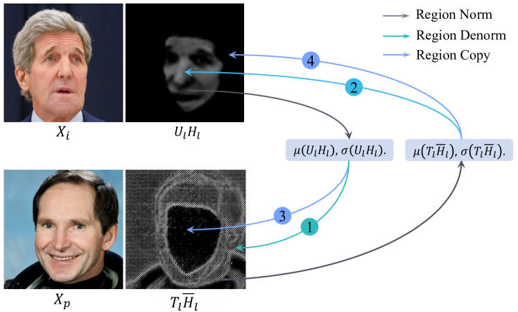
Generator . The rendered 3D face and the appearance embedding feature map are input to to synthesize the video frame . For the better fusion result, we propose a novel region-aware conditional normalization layer (RCN) layer tailored for our network as presented in Fig 4. In general, RCN computes the mean and variance for facial and non-facial areas respectively and conducts the denormalization in both the same-regional retention or cross-regional transfer way. Specifically, for the same-region retention term, we firstly apply batch normalization and then copy the region features to the corresponding parts. For the cross-regional term, we transfer the region statistic to the counterpart with a relatively small weight.
For each feature map in the upsampling process of , , where is the number of upsampling layers, RCN is expressed as follows.
| (6) |
and follows AdaIN as:
| (7) |
where is an upsampled version of the appearance feature map and is a downsampled version of the facial mask . indicates the non-facial area. Two learnable parameter vectors and are adopted for balance. and share the same channel as input . Each element and , and the initialization values are set to 0.8 and 0.1, respectively.
Why should the denormalization process be limited in the specific region? AdaIN [26] treats elements in the same channel equally and aligns the channel-wise mean and variance. SPADE [27] predicts pixel-level affine parameters and applies spatial-aware denormalization. However, in our case, since Generator and Appearance Embedder encode the facial and non-facial areas respectively, restricting the computation in specific areas gives more accurate statistics and avoids the interference of meaningless feature regions. Why should we need a cross-regional transfer term? This cross-regional transfer term applies the facial statistic to the non-facial areas with a relatively small weight and vice versa. This mechanism makes the two regions adjust to each other and when training end-to-end, it leads to more context-harmonious results.
Discriminator . Following pix2pixHD [28], we adopt the same multi-scale discriminator and loss functions, except that we replace the least squared loss term [29] by the hinge loss term [30].
| Mode | Model | FID | SSIM | |||
|---|---|---|---|---|---|---|
| Swapping | FaceShifter | 52.1 | - | 1.31 | (4.31, 3.26, 1.13) | 4.43 |
| FSGAN | 45.9 | - | 0.89 | (2.27, 3.21, 0.76) | 3.23 | |
| UniFaceGAN | 34.1 | - | 0.26 | (1.12, 1.31, 0.65) | 2.31 | |
| Reenactment | X2face | 52.1 | 0.05 | 0.29 | (2.31, 1.26, 0.90) | 4.43 |
| FSGAN | 32.4 | 0.23 | 0.10 | (1.43, 0.75, 0.90) | 3.58 | |
| FTH | 43.1 | 0.18 | 0.43 | (1.50, 1.23, 0.81) | 5.67 | |
| FOMM | 28.2 | 0.59 | 0.12 | (0.76, 0.54, 0.12) | 4.02 | |
| Fast Bi-layer | 45.8 | 0.22 | 0.14 | (0.23, 0.34, 0.12) | 3.87 | |
| UniFaceGAN | 24.4 | 0.82 | 0.12 | (0.21, 0.25, 0.12) | 3.12 |
| Mode | FID | SSIM | |||||
|---|---|---|---|---|---|---|---|
| Swapping | 0.0 | 34.5 | - | 0.28 | (1.31, 1.33, 0.42) | 2.18 | 4.23 |
| 0.2 | 34.3 | - | 0.26 | (1.12, 1.30, 0.65) | 2.20 | 4.01 | |
| 0.4 | 34.1 | - | 0.27 | (1.11, 1.33, 0.65) | 2.23 | 3.74 | |
| 0.5 | 34.1 | - | 0.26 | (1.12, 1.31, 0.65) | 2.31 | 3.54 | |
| 0.6 | 36.3 | - | 0.51 | (1.18, 1.31, 0.64) | 2.48 | 3.49 | |
| 0.8 | 38.2 | - | 1.02 | (1.20, 1.32, 0.65) | 2.56 | 3.45 | |
| Reenactment | 0.2 | 25.1 | 0.80 | 0.31 | (0.42, 0.38, 0.12) | 4.01 | 4.03 |
| 0.4 | 24.8 | 0.81 | 0.26 | (0.40, 0.34, 0.11) | 3.30 | 3.82 | |
| 0.5 | 24.4 | 0.82 | 0.12 | (0.21, 0.25, 0.12) | 3.12 | 3.65 | |
| 0.6 | 26.1 | 0.85 | 0.29 | (0.27, 0.31, 0.12) | 3.92 | 3.62 | |
| 0.8 | 26.5 | 0.86 | 0.32 | (0.30, 0.32, 0.15) | 4.08 | 3.56 | |
| 1.0 | 26.9 | 0.87 | 0.33 | (0.31, 0.33, 0.15) | 4.11 | 3.25 |


III-D Loss Function
Appearance Preserving Loss. The generated facial image should have the same appearance information as and the appearance preserving loss is measured in norm as follows:
| (8) |
where is the appearance embedder described in Section III-C.
Reconstruction Loss. When the dynamic training sample selection mechanism chooses the intra-video sampling, we have ground truths for supervised training, since and are from the same person. Then we have the reconstruction loss as follows:
| (9) |
Note that for the inter-video sampling case, is set to 0.
Adversarial Loss. For , we use a multi-scale adversarial loss [28] on the downsampled output image to enforce photo-realistic results:
| (10) |
where and are the downsampled versions of and , respectively, and is the total number of scale versions.
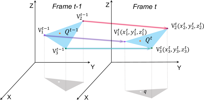
3D Temporal Loss. Insipred by [31], we introduce a flow-based 3D temporal loss to alleviate the inter-frame flicker artifacts. The main difficulty lies in how to generate the dense optical flow map between two consecutive frames. Here, we propose a 3D-based optical flow extraction method, which avoids the use of flow estimation networks [32].
Thanks to 3DMM, the optical flow values for reconstructed vertices can be easily obtained by directly subtracting 3D coordinates between adjacent frames. To obtain the dense flow map, we propose to conduct barycentric coordinate interpolation for each pixel in the 2D pixel domain. As shown in Fig. 3(a), for a query point with location , we find the triangle with its - plane projection version containing . Let , , be the vertices of . We compute the barycentric coordinates of , with respect to . Therefore, the flow value at position is calculated as follows:
| (11) |
Then we need to obtain visibility maps . Let and be the depth buffer generated by 3DDFA. For frame , we interpolate the depth of to get the coordinate of :
| (12) |
where denotes the component of . Since the depth buffer denotes the minimum visible z value of each coordinate of the 2D pane to project on, the visibility map value at is given as:
| (15) |
where means the depth buffer value of at point . For frame , we compute the coordinate of as follows:
| (16) |
Since and are known, we can obtain , , (i.e. , , components of ). Then the calculation of visibility map for frame at position is similar to .
| (19) |
Finally, the optical flow map between two consecutive frames is given as follows:
| (20) |
Therefore, we define the 3D temporal loss between and in the format of mean squared error:
| (21) |
where is the warping function that warps the output at time back to time . The overall loss function is thus reached as :
| (22) |
where , , and are the weights to balance different terms, which are set to 10, 1, 10 and 5 in our experiments, respectively.
IV Experiments


IV-A Experiment Details
In this paper, the Voxceleb2 [33] dataset is adopted to conduct the multi-task training. Voxceleb2 is among the largest available video datasets, which covers over a million utterances from over 6,000 speakers. The intra-video sampling rate is set to 0.5. Quantitative comparisons are conducted with respect to five metrics: Frechet-inception distance (FID) [34], structured similarity (SSIM) [35], identity error , pose error , and expression error . More about the training details, evaluation metrics and the network architecture are available in the supplementary material.
IV-B Comparison Results
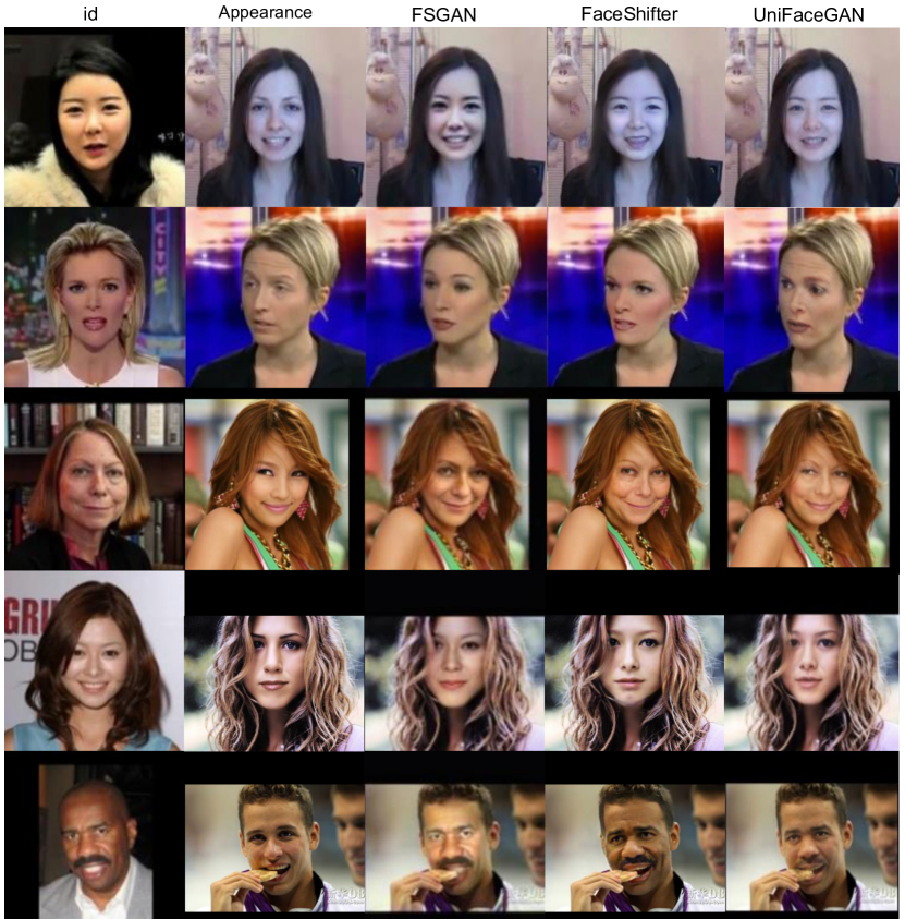
Face swapping. When setting and crop out of , it falls into the face swapping problem. Fig. 5 presents qualitative results against FaceShifter [20] and FSGAN [6]. UniFaceGAN generates high-fidelity results, even under challenging cases with varying ages, poses, gender and occlusions. The results of FSGAN are obviously blurred and over-smooth while FaceShiter suffers from striped flaws. Besides, quantitative results in Table I also show that UniFaceGAN achieves better performance, which means our proposed UniFaceGAN is more photo-realistic and accurately captures the pose and expression information. To make fair comparisons, we compare our UniFaceGAN with FSGAN and Faceshifter using the cases presented in their paper and the results are shown in Figure. 8. Note that we just infer on the images and do not fine tune our model on the corresponding datasets (e.g. Caltech Occluded Faces in the Wild (COFW) [36], IJB-C [37], VGGFace [38] datasets, etc).
Face reenactment. To deal with the face reenactment task, we set and crop out of or sample and in the same videos. Table I and Fig 6 show the comparison results with state-of-the-art video face reenactment methods. FSGAN, FOMM [39] and Fast Bi-layer [40] suffer from the blur background and UniFaceGAN settles this obstacle by explicitly providing an appearance hint. X2face shows a distorted face which is a common problem for warping-based methods. FTH can not animate the target person accurately, which demonstrates that our 3D-to-2D method is superior to the 2D landmark-based methods.
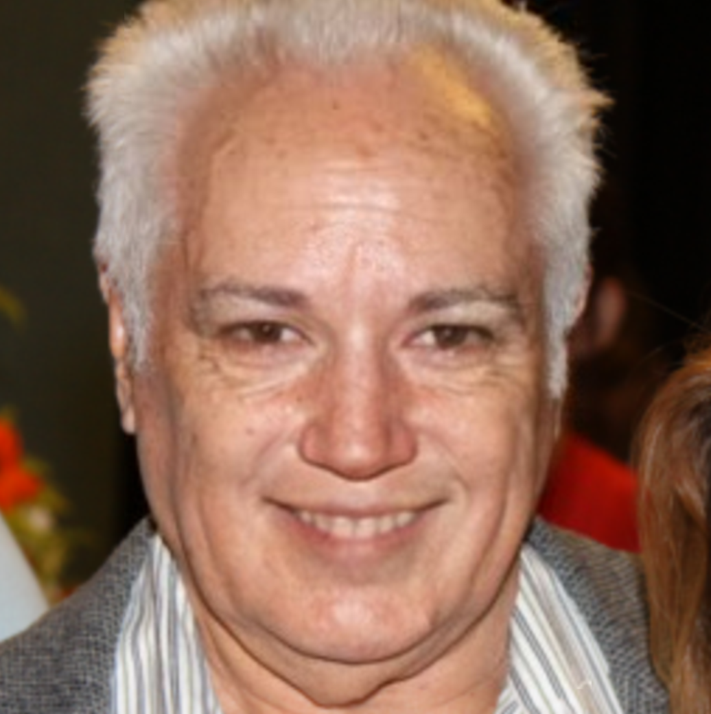
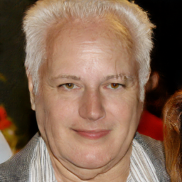
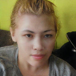
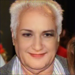
Fully disentangled manipulation. When , and are of different identities, we perform a novel fully disentangled manipulation task. The results in Fig. 7 show that the generated portrait image successfully mixes information of identity, appearance and expression from different source images.
IV-C Ablation Studies
Ablation studies on DTSS:
W and W/O dynamic training sample selection (DTSS). DTSS selects the identity image , the appearance image and the expression image in two ways. We shift the intra-video sampling ratio manually and the results are listed in Table II. Intuitively, decreases with the increase of , since our 3D temporal loss is only applied in the intra-video case where , and are sampled from the same video. SSIM is evaluated in the self-driving scenario and when increases, SSIM increases naturally. The other evaluation criteria generally achieve the best scores when setting to 0.5 for both the face swapping and the face reenactment task. Specifically, when the ratio is set to 0, the whole framework falls into a face swapping pipeline. Similarly, setting to 1, UniFaceGAN can only handle the face reenactment task. The comparison results between and or indicate that this multi-task training is more effective than training the single task alone.
Ablation studies on the loss functions:
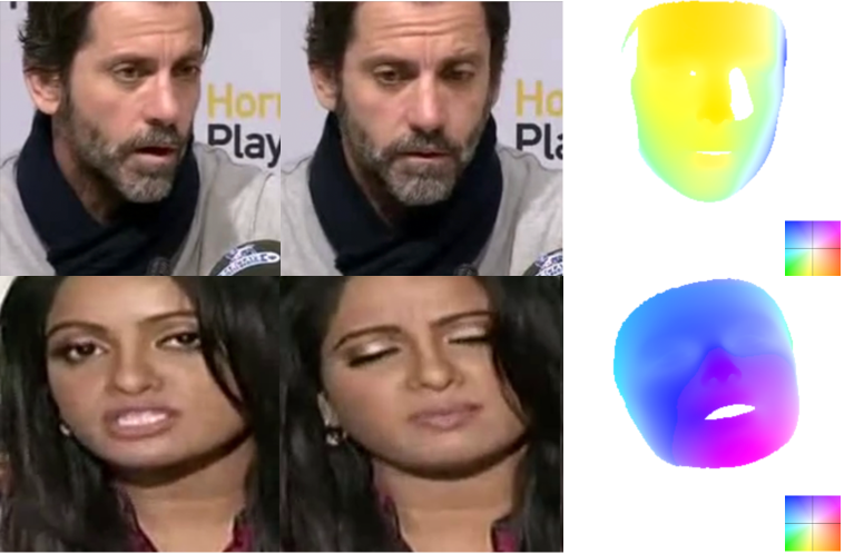
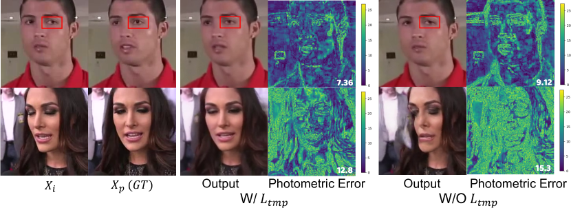
1) W and W/O temporal consistency loss. The ablation study of our 3D temporal loss is available in Table III. Here we evaluate in the scenario of self-driving reenactment since only in this case we have the ground truth. Several cases are shown in Fig 9 and photometric error [1] is also computed between output and ground truth. Fig 9 shows that plays a significantly role especially when and have large pose variations.
2) Dense flow vs. Sparse flow. vs. FlowNet2. To demonstrate the necessity of obtaining the dense optical flow maps using the barycentric coordinate interpolation, we compare UniFaceGAN with the models which only use sparse optical flow as temporal constraints. is still calculated by Equation 21, but using the sparse optical flow map instead. Specifically, for each vertex of 3DMM reconstruction output, we project its optical flow value to the 2D plane orthogonally and predict the visibility according to the Z-Buffer value. Table III gives the results of using sparse flow maps and the results show training with dense flow maps outperforms the sparse ones. In Table III, we also compute the temporal loss using the optical flow estimation network FlowNet2 [32]. It shows that the optical flow computed by FlowNet2 leads to even worse results and this may be caused by the inaccurate facial optical flow estimation by FlowNet2.
| Task | Model | FID | SSIM | ||||
|---|---|---|---|---|---|---|---|
| Swapping | W/O | 43.2 | - | 0.93 | (1.61,1.42,0.66) | 3.36 | 5.67 |
| FlowNet2 | 50.2 | - | 1.34 | (1.63,1.73,0.66) | 3.76 | 5.94 | |
| Sparse | 38.2 | - | 0.73 | (1.34,1.54,0.66) | 2.86 | 4.23 | |
| Dense(Ours) | 34.1 | - | 0.26 | (1.12,1.31,0.65) | 2.31 | 3.54 | |
| Reenactment | W/O | 38.3 | 0.65 | 0.27 | (0.43,0.38,0.12) | 3.93 | 6.91 |
| FlowNet2 | 44.1 | 0.49 | 0.33 | (0.50,0.53,0.17) | 5.65 | 8.24 | |
| Sparse | 30.0 | 0.75 | 0.17 | (0.46,0.39,0.14) | 3.52 | 6.54 | |
| Dense(Ours) | 24.4 | 0.82 | 0.12 | (0.21,0.25,0.12) | 3.12 | 3.65 |
3) W and W/O Appearance Preserving Loss or Reconstruction Loss. The experimental results in Table IV show that either dropping or leads to consistent performance degradation. The qualitative comparison results are also shown in Fig. 12. When dropping , the output images suffer from the blurry background (especially the hair regions); When dropping , the quality of the output image is greatly affected (e.g., the unnatural transitions between face and background).
| Task | FID | SSIM | |||||
|---|---|---|---|---|---|---|---|
| swapping | ✓ | 41.4 | - | 0.39 | (1.17,1.45,0.67) | 2.71 | |
| ✓ | 38.7 | - | 0.34 | (1.17,1.35,0.66) | 2.54 | ||
| ✓ | ✓ | 34.1 | - | 0.26 | (1.12,1.31,0.65) | 2.31 | |
| Reenactment | ✓ | 30.2 | 0.71 | 0.19 | (0.22,0.26,0.12) | 4.98 | |
| ✓ | 28.6 | 0.74 | 0.15 | (0.23,0.26,0.12) | 4.03 | ||
| ✓ | ✓ | 24.4 | 0.82 | 0.12 | (0.21,0.25,0.12) | 3.12 |
4) Removing the self-attention module in G. In the experiment, we add the self-attention module at the resolution in the up-sampling part of the generator. To prove its necessity, we conduct the ablation studies without the self-attention module. The quantitative comparison results are shown Table V. The results show that the inserted self-attention module improves the quality of the outputs greatly. For better illustrations, the qualitative comparison results are shown between Fig. 12(c) and Fig. 12(f).
5) Long Term Temporal Loss Constraint. We investigate the influence of long term temporal loss. Specifically, we set the input frames to be and , and remain the datasets and the pipeline unchanged. The quantitative results are available in the supplementary material.
| Task | self-attention | FID | SSIM | |||
|---|---|---|---|---|---|---|
| swapping | 39.2 | - | 0.41 | (1.18,1.51,0.67) | 2.67 | |
| ✓ | 34.1 | - | 0.26 | (1.12,1.31,0.65) | 2.31 | |
| Reenactment | 29.7 | 0.64 | 0.23 | (0.24,0.28,0.13) | 3.65 | |
| ✓ | 24.4 | 0.82 | 0.12 | (0.21,0.25,0.12) | 3.12 |

Ablation studies for RCN:
1) RCN vs. AdaIN vs. SPADE. When replacing RCN with AdaIN or SPADE, the fidelity restoration of UniFaceGAN degrades substantially. The quantitative and qualitative comparison results in Table VI (a) and Fig 10 show that RCN leads to a more smooth transition between the facial and non-facial areas and looks more context-harmonious.
2) Are the cross-regional term and same-regional term necessary? We have added more ablation studies for RCN, i.e., experiments with only same-regional retention term or cross-regional transfer term. The quantitative and qualitative results are shown Table VI (b) and Fig. 10. The experimental results demonstrate that both the same-regional retention term or cross-regional transfer terms are crucial to the photo-realistic outputs. The output without the cross-regional transfer term (Fig. 10(f)) has unsmooth boundary transitions between facial and non-facial parts. Besides, removing the same-regional retention term leads to the color contaminate, e.g., Fig. 10(g) facial part has the black shadow which may be transferred from the background of appearance image in Fig. 10(b).
3) Are just facial or non-facial related terms necessary? In Eqn. 6, the second () and the third () terms contribute to the generated facial part and they are called facial related terms here. Similarly, the first () and the fourth () term are called non-facial related terms. We conduct comparison experiments with only facial region term or no-facial region transfer term. The quantitative and qualitative results are shown Table VI (c) and Fig. 11. The experimental results show that with only facial related items, the generated results suffer from the blurry background and color inconsistency and with only non-facial related items, the output can not generate the clear facial parts. All the loss term ablation studies are trained from scratch and remain the experimental settings unchanged.
| (a) | Mode | FID | SSIM | |||
|---|---|---|---|---|---|---|
| Swapping | RCN(Ours) | 34.1 | - | 0.26 | (1.12,1.31,0.65) | 2.31 |
| AdaIN | 47.2 | - | 0.59 | (1.12,1.43,0.66) | 2.72 | |
| SPADE | 39.5 | - | 0.50 | (1.11,1.33,0.65) | 2.55 | |
| Reenactment | RCN(Ours) | 24.4 | 0.82 | 0.12 | (0.21,0.25,0.12) | 3.12 |
| AdaIN | 36.9 | 0.72 | 0.18 | (0.21,0.32,0.12) | 3.52 | |
| SPADE | 32.1 | 0.76 | 0.18 | (0.21,0.27,0.12) | 3.38 | |
| (b) | Mode | FID | SSIM | |||
| swapping | Cross only | 44.2 | - | 0.51 | (1.20,1.47,0.67) | 3.06 |
| Same only | 40.3 | - | 0.45 | (1.18,1.41,0.66) | 2.63 | |
| Full(Ours) | 34.1 | - | 0.26 | (1.12,1.31,0.65) | 2.31 | |
| Reenactment | Cross only | 31.6 | 0.58 | 0.23 | (0.24,0.26,0.13) | 3.70 |
| Same only | 30.2 | 0.64 | 0.17 | (0.25,0.26,0.12) | 3.51 | |
| Full(Ours) | 24.4 | 0.82 | 0.12 | (0.21,0.25,0.12) | 3.12 | |
| (c) | Mode | FID | SSIM | |||
| swapping | Facial only | 50.9 | - | 0.73 | (1.15,1.40,0.67) | 4.23 |
| Non-facial only | 49.3 | - | 0.86 | (1.15,1.38,0.66) | 5.34 | |
| Full(Ours) | 34.1 | - | 0.26 | (1.12,1.31,0.65) | 2.31 | |
| Reenactment | Facial only | 37.3 | 0.29 | 0.40 | (0.24,0.28,0.13) | 4.32 |
| Non-facial only | 35.1 | 0.36 | 0.35 | (0.24,0.28,0.12) | 3.83 | |
| Full(Ours) | 24.4 | 0.82 | 0.12 | (0.21,0.25,0.12) | 3.12 |
V Conclusions
In this work, we have proposed a unified framework called UniFaceGAN for handling multiple video portrait manipulation tasks and generating temporally consistent outputs. To be specific, we carefully design a Dynamic Training Sample Selection mechanism to facilitate this multi-task training. A novel 3D temporal loss is proposed to enforce the visual consistency in synthesized videos. Besides, we further introduce a region-aware conditional normalization (RCN) layer to achieve the better face blending. The extensive experiments have demonstrated the consistent superiority of the proposed framework across multiple tasks over the state-of-the-art methods.
References
- [1] Hyeongwoo Kim, Pablo Garrido, Ayush Tewari, Weipeng Xu, Justus Thies, Matthias Nießner, Patrick Pérez, Christian Richardt, Michael Zollhöfer, and Christian Theobalt. Deep video portraits. ACM Transactions on Graphics (TOG), 37(4):1–14, 2018.
- [2] Kyle Olszewski, Zimo Li, Chao Yang, Yi Zhou, Ronald Yu, Zeng Huang, Sitao Xiang, Shunsuke Saito, Pushmeet Kohli, and Hao Li. Realistic dynamic facial textures from a single image using gans. In Proceedings of the IEEE International Conference on Computer Vision, pages 5429–5438, 2017.
- [3] Iryna Korshunova, Wenzhe Shi, Joni Dambre, and Lucas Theis. Fast face-swap using convolutional neural networks. In Proceedings of the IEEE International Conference on Computer Vision, pages 3677–3685, 2017.
- [4] Yuval Nirkin, Iacopo Masi, Anh Tran Tuan, Tal Hassner, and Gerard Medioni. On face segmentation, face swapping, and face perception. In 2018 13th IEEE International Conference on Automatic Face & Gesture Recognition (FG 2018), pages 98–105. IEEE, 2018.
- [5] Xiaohan Jin, Ye Qi, and Shangxuan Wu. Cyclegan face-off. arXiv preprint arXiv:1712.03451, 2017.
- [6] Yuval Nirkin, Yosi Keller, and Tal Hassner. Fsgan: Subject agnostic face swapping and reenactment. In Proceedings of the IEEE International Conference on Computer Vision, pages 7184–7193, 2019.
- [7] Pablo Garrido, Levi Valgaerts, Ole Rehmsen, Thorsten Thormahlen, Patrick Perez, and Christian Theobalt. Automatic face reenactment. In Proceedings of the IEEE Conference on Computer Vision and Pattern Recognition, pages 4217–4224, 2014.
- [8] Justus Thies, Michael Zollhofer, Marc Stamminger, Christian Theobalt, and Matthias Nießner. Face2face: Real-time face capture and reenactment of rgb videos. In Proceedings of the IEEE conference on computer vision and pattern recognition, pages 2387–2395, 2016.
- [9] Supasorn Suwajanakorn, Steven M Seitz, and Ira Kemelmacher-Shlizerman. Synthesizing obama: learning lip sync from audio. ACM Transactions on Graphics (TOG), 36(4):1–13, 2017.
- [10] Hadar Averbuch-Elor, Daniel Cohen-Or, Johannes Kopf, and Michael F Cohen. Bringing portraits to life. ACM Transactions on Graphics (TOG), 36(6):196, 2017.
- [11] Olivia Wiles, A Sophia Koepke, and Andrew Zisserman. X2face: A network for controlling face generation using images, audio, and pose codes. In Proceedings of the European Conference on Computer Vision (ECCV), pages 670–686, 2018.
- [12] Aliaksandr Siarohin, Stéphane Lathuilière, Sergey Tulyakov, Elisa Ricci, and Nicu Sebe. Animating arbitrary objects via deep motion transfer. In Proceedings of the IEEE Conference on Computer Vision and Pattern Recognition, pages 2377–2386, 2019.
- [13] Wayne Wu, Yunxuan Zhang, Cheng Li, Chen Qian, and Chen Change Loy. Reenactgan: Learning to reenact faces via boundary transfer. In Proceedings of the European Conference on Computer Vision (ECCV), pages 603–619, 2018.
- [14] Egor Zakharov, Aliaksandra Shysheya, Egor Burkov, and Victor Lempitsky. Few-shot adversarial learning of realistic neural talking head models. In Proceedings of the IEEE International Conference on Computer Vision, pages 9459–9468, 2019.
- [15] Jian Zhao, Lin Xiong, Panasonic Karlekar Jayashree, Jianshu Li, Fang Zhao, Zhecan Wang, Panasonic Sugiri Pranata, Panasonic Shengmei Shen, Shuicheng Yan, and Jiashi Feng. Dual-agent gans for photorealistic and identity preserving profile face synthesis. In Advances in neural information processing systems, pages 66–76, 2017.
- [16] Volker Blanz and Thomas Vetter. A morphable model for the synthesis of 3d faces. In Proceedings of the 26th annual conference on Computer graphics and interactive techniques, pages 187–194, 1999.
- [17] Xiangyu Zhu, Zhen Lei, Xiaoming Liu, Hailin Shi, and Stan Z Li. Face alignment across large poses: A 3d solution. In Proceedings of the IEEE conference on computer vision and pattern recognition, pages 146–155, 2016.
- [18] Koki Nagano, Jaewoo Seo, Jun Xing, Lingyu Wei, Zimo Li, Shunsuke Saito, Aviral Agarwal, Jens Fursund, and Hao Li. pagan: real-time avatars using dynamic textures. ACM Transactions on Graphics (TOG), 37(6):1–12, 2018.
- [19] Sungjoo Ha, Martin Kersner, Beomsu Kim, Seokjun Seo, and Dongyoung Kim. Marionette: Few-shot face reenactment preserving identity of unseen targets. arXiv preprint arXiv:1911.08139, 2019.
- [20] Lingzhi Li, Jianmin Bao, Hao Yang, Dong Chen, and Fang Wen. Faceshifter: Towards high fidelity and occlusion aware face swapping. arXiv preprint arXiv:1912.13457, 2019.
- [21] Volker Blanz, Kristina Scherbaum, Thomas Vetter, and Hans-Peter Seidel. Exchanging faces in images. In Computer Graphics Forum, volume 23, pages 669–676. Wiley Online Library, 2004.
- [22] Jianmin Bao, Dong Chen, Fang Wen, Houqiang Li, and Gang Hua. Towards open-set identity preserving face synthesis. In Proceedings of the IEEE Conference on Computer Vision and Pattern Recognition, pages 6713–6722, 2018.
- [23] Xiangyu Zhu, Xiaoming Liu, Zhen Lei, and Stan Z Li. Face alignment in full pose range: A 3d total solution. IEEE transactions on pattern analysis and machine intelligence, 41(1):78–92, 2017.
- [24] Pascal Paysan, Reinhard Knothe, Brian Amberg, Sami Romdhani, and Thomas Vetter. A 3d face model for pose and illumination invariant face recognition. In 2009 Sixth IEEE International Conference on Advanced Video and Signal Based Surveillance, pages 296–301. Ieee, 2009.
- [25] Chen Cao, Yanlin Weng, Shun Zhou, Yiying Tong, and Kun Zhou. Facewarehouse: A 3d facial expression database for visual computing. IEEE Transactions on Visualization and Computer Graphics, 20(3):413–425, 2013.
- [26] Xun Huang and Serge Belongie. Arbitrary style transfer in real-time with adaptive instance normalization. In Proceedings of the IEEE International Conference on Computer Vision, pages 1501–1510, 2017.
- [27] Taesung Park, Ming-Yu Liu, Ting-Chun Wang, and Jun-Yan Zhu. Semantic image synthesis with spatially-adaptive normalization. In Proceedings of the IEEE Conference on Computer Vision and Pattern Recognition, pages 2337–2346, 2019.
- [28] Ting-Chun Wang, Ming-Yu Liu, Jun-Yan Zhu, Andrew Tao, Jan Kautz, and Bryan Catanzaro. High-resolution image synthesis and semantic manipulation with conditional gans. In Proceedings of the IEEE conference on computer vision and pattern recognition, pages 8798–8807, 2018.
- [29] Xudong Mao, Qing Li, Haoran Xie, Raymond YK Lau, Zhen Wang, and Stephen Paul Smolley. Least squares generative adversarial networks. In Proceedings of the IEEE International Conference on Computer Vision, pages 2794–2802, 2017.
- [30] Jae Hyun Lim and Jong Chul Ye. Geometric gan. arXiv preprint arXiv:1705.02894, 2017.
- [31] Xuanyi Dong, Shoou-I Yu, Xinshuo Weng, Shih-En Wei, Yi Yang, and Yaser Sheikh. Supervision-by-registration: An unsupervised approach to improve the precision of facial landmark detectors. In Proceedings of the IEEE Conference on Computer Vision and Pattern Recognition, pages 360–368, 2018.
- [32] Eddy Ilg, Nikolaus Mayer, Tonmoy Saikia, Margret Keuper, Alexey Dosovitskiy, and Thomas Brox. Flownet 2.0: Evolution of optical flow estimation with deep networks. In Proceedings of the IEEE conference on computer vision and pattern recognition, pages 2462–2470, 2017.
- [33] Joon Son Chung, Arsha Nagrani, and Andrew Zisserman. Voxceleb2: Deep speaker recognition. arXiv preprint arXiv:1806.05622, 2018.
- [34] Martin Heusel, Hubert Ramsauer, Thomas Unterthiner, Bernhard Nessler, and Sepp Hochreiter. Gans trained by a two time-scale update rule converge to a local nash equilibrium. In Advances in neural information processing systems, pages 6626–6637, 2017.
- [35] Zhou Wang, Alan C Bovik, Hamid R Sheikh, and Eero P Simoncelli. Image quality assessment: from error visibility to structural similarity. IEEE transactions on image processing, 13(4):600–612, 2004.
- [36] Xavier P Burgos-Artizzu, Pietro Perona, and Piotr Dollár. Robust face landmark estimation under occlusion. In Proceedings of the IEEE international conference on computer vision, pages 1513–1520, 2013.
- [37] Brianna Maze, Jocelyn Adams, James A Duncan, Nathan Kalka, Tim Miller, Charles Otto, Anil K Jain, W Tyler Niggel, Janet Anderson, Jordan Cheney, et al. Iarpa janus benchmark-c: Face dataset and protocol. In 2018 International Conference on Biometrics (ICB), pages 158–165. IEEE, 2018.
- [38] Omkar M Parkhi, Andrea Vedaldi, and Andrew Zisserman. Deep face recognition. 2015.
- [39] Aliaksandr Siarohin, Stéphane Lathuilière, Sergey Tulyakov, Elisa Ricci, and Nicu Sebe. First order motion model for image animation. In Advances in Neural Information Processing Systems, pages 7137–7147, 2019.
- [40] Egor Zakharov, Aleksei Ivakhnenko, Aliaksandra Shysheya, and Victor Lempitsky. Fast bi-layer neural synthesis of one-shot realistic head avatars. In European Conference on Computer Vision, pages 524–540. Springer, 2020.