SDSS-IV MaNGA: Stellar M/L gradients and the M/L-colour relation in galaxies

Abstract

The stellar mass-to-light ratio gradient in SDSS $r-$band $\nabla(M_{*}/L_{r})$ of a galaxy depends on its mass assembly history, which is imprinted in its morphology and gradients of age, metallicity, and stellar initial mass function (IMF). Taking a MaNGA sample of 2051 galaxies with stellar masses ranging from $10^{9}$ to $10^{12}M_{\odot}$ released in SDSS DR15, we focus on face-on galaxies, without merger and bar signatures, and investigate the dependence of the 2D $\nabla(M_{*}/L_{r})$ on other galaxy properties, including $M_{*}/L_{r}$-colour relationships by assuming a fixed Salpeter IMF as the mass normalization reference. The median gradient is $\nabla M_{*}/L_{r}\sim-0.1$ (i.e., the $M_{*}/L_{r}$ is larger at the centre) for massive galaxies, becomes flat around $M_{*}\sim 10^{10}M_{\odot}$ and change sign to $\nabla M_{*}/L_{r}\sim 0.1$ at the lowest masses. The $M_{*}/L_{r}$ inside a half light radius increases with increasing galaxy stellar mass; in each mass bin, early-type galaxies have the highest value, while pure-disk late-type galaxies have the smallest. Correlation analyses suggest that the mass-weighted stellar age is the dominant parameter influencing the $M_{*}/L_{r}$ profile, since a luminosity-weighted age is easily affected by star formation when the specific star formation rate (sSFR) inside the half light radius is higher than $10^{-3}{\rm Gyr}^{-1}$. With increased sSFR gradient, one can obtain a steeper negative $\nabla(M_{*}/L_{r})$. The scatter in the slopes of $M_{*}/L$-colour relations increases with increasing sSFR, for example, the slope for post-starburst galaxies can be flattened to $0.45$ from the global value $0.87$ in the $M_{*}/L$ vs. $g-r$ diagram. Hence converting galaxy colours to $M_{*}/L$ should be done carefully, especially for those galaxies with young luminosity-weighted stellar ages, which can have quite different star formation histories.

1 Introduction

The stellar mass assembly history of a galaxy is one of the key parameters for understanding its formation and evolution processes. An important first step is to understand what the stellar mass of a galaxy is from the observations we take. At optical wavelengths, we define a simple multiplicative relationship between the light received from a galaxy and its mass, the stellar mass-to-light ratio $M_{*}/L$. Currently, we have three different ways of estimating the mass-to-light ratios and thus galaxy stellar masses.

The first method involves performing a stellar population analysis on the observed galaxy spectra or broad band spectral energy distributions (SEDs), and calculating the stellar mass based on fitted weights to a series of stellar population templates with different stellar mass-to-light ratios ($M_{*}/L$) (see the review by Conroy, 2013).

The second converts the galaxy luminosity ($L$) at a specific wavelength band to stellar mass by employing an empirical stellar mass-to-light ratio to colour relationship (e.g. Bell et al., 2003; Gallazzi & Bell, 2009; Du et al., 2019).

The third method uses dynamical modelling of a galaxy to obtain $M_{*}/L$. For simplicity, the ratio is often assumed to be constant over the whole galaxy, and is taken as a free parameter when seeking to reproduce a galaxy’s 2D stellar kinematic maps (e.g. Cappellari et al., 2006, 2013; Thomas et al., 2011; Cappellari, 2016; Li et al., 2017; Lu et al., 2020).

When applying stellar population analysis to obtain a $M_{*}/L$, the accuracy depends on both the fitting algorithm and stellar population models. The empirical $M_{*}/L$-colour relation also depends on how well $M_{*}/L$ can be fitted. In the galaxy dynamical modelling, the stellar masses are not affected by any uncertainties in stellar population analysis, but methods are affected by a stellar and dark matter mass degeneracy and the assumption of a constant $M_{*}/L$ may not be robust.

In the literature, radial $M_{*}/L$ gradients of galaxies are mainly obtained from stellar population analyses of spatially resolved spectra or broad band SEDs by assuming a constant initial mass function (IMF). For example, Tortora et al. (2011) performed SED fitting to SDSS $ugriz$ bands and found that the $M_{*}/L$ gradients vary with galaxy stellar mass. Assuming a fixed IMF, the MaNGA work by Li et al. (2018) (see their Figure 6) found that the $M_{*}/L$ gradients tend to follow the age gradients: the $M_{*}/L$ gradient is nearly flat or implies a larger $M_{*}/L$ in the centre for older galaxies and a larger M/L in the outer parts for younger ones. Massive elliptical galaxies can also have negative $M_{*}/L$ gradients, e.g., Szomoru et al. (2013), Newman, Ellis, & Treu (2015). Sonnenfeld et al. (2018) obtained gradients by using three different methods: $u-g$ colour versus $M_{*}/L$ relation, $U-B-V$ colours versus $M_{*}/L$ relation, weak and strong lensing modelling resulting in three different negative values of $-0.13$, $-0.15$, and $-0.24$, respectively. CALIFA (Sanchez et al., 2012) galaxies with morphologies ranging from E0 to Sd types have their $M_{*}/L$ gradients steeper than $-0.2$ in the inner regions and nearly flat in the outer regions (García-Benito et al., 2019).

Galaxy $M_{*}/L$ gradients can not only be estimated by spatially resolved photometric or spectroscopic data, but also predicted using galaxy formation and evolution models. From theoretical (e.g. White & Rees, 1978; Hopkins et al., 2009, 2010; Oser et al., 2010, 2012) and observational (e.g. Bezanson et al., 2009; Naab, 2013; Martin-Navarro et al., 2018) studies, the formation and evolution of elliptical and bulge-dominated spiral galaxies usually occur through two distinct phases, i.e., first a “monolithic” collapse phase to form the “in situ” stars (e.g. Eggen et al., 1962; Larson, 1974), and a second merger-driven growth phase to accrete “ex situ” stars (e.g. Ciotti et al., 2007; Oser et al., 2012; Rodriguez-Gomez et al., 2016). This two-phase scenario suggests that these galaxies possibly have varying radial gradients of stellar population parameters, including stellar age, metallicity, and IMF, which are exactly the three parameters that determine a $M_{*}/L$ from a spectrum.

For early type galaxies (ETGs), including both ellipticals (E) and lenticulars (S0), Kuntschner et al. (2010) and Li et al. (2018) consistently show that the age gradients are nearly flat for older ETGs (see also Zheng et al., 2017; Martin-Navarro et al., 2018), while younger ETGs tend to have younger cores, likely associated to residual star formation in the centres. González Delgado et al. (2015) found negative age gradients inside a half light radius (HLR), but nearly flat ones beyond 2 HLR. Positive age gradients can be obtained by changing the sample and data analysis methods (e.g. Koleva et al., 2011; Tortora et al., 2011; Goddard et al., 2017). For late type galaxies (LTGs), galaxies with higher stellar masses tend to have steeper negative age gradients, and those with lower masses have their gradients varying from negative, nearly flat, to positive gradients (e.g. Tortora et al., 2011; Pérez et al., 2013; González Delgado et al., 2015; Zheng et al., 2017).

Statistically, ETGs and LTGs have negative metallicity gradients in logarithmic radius, with the values ranging from $-0.5$ to 0 (e.g. Mehlert et al., 2003; Spolaor et al., 2009; Kuntschner et al., 2010; González Delgado et al., 2015; Goddard et al., 2017; Zheng et al., 2017; Li et al., 2018; Martin-Navarro et al., 2018; Zibetti et al., 2020).

Evidence of IMF variation has been presented by different authors. Initial convincing evidence for an IMF heavier than the Milky Way’s in massive ETGs was inferred by modelling stellar absorption lines by van Dokkum & Conroy (2010). This result appeared consistent with similar evidence from mass determinations using strong lensing (Auger et al., 2010). Dynamical modelling of the Atlas3D sample by Cappellari et al. (2012) indicated a systematic trend in the IMF, going from Milky-Way like in the low velocity dispersion and younger ETGs to Salpeter-like or heavier for the high dispersion and older ETGs. A systematic trend was subsequently also inferred from stellar population analyses by Ferreras et al. (2013); Spiniello et al. (2014); Conroy et al. (2017); Li et al. (2017); Parikh et al. (2018); Vaughan et al. (2018b), and Zhou et al. (2019), although some studies found no clear evidence (e.g. Zieleniewski, 2017; Alton, Smith & Lucey, 2018; Vaughan et al., 2018a). A recent review of the consistency and tension in IMF determination studies is given by Smith (2020).

In this paper, we will use SDSS-IV/MaNGA (Bundy et al., 2015) IFS data to study $M_{*}/L$ gradients driven by age and metallicity gradients under a fixed Salpeter IMF assumption, and investigate how they affect stellar mass estimations and $M_{*}/L$-colour relations. Our spectral fitting code and libraries, and data analysis processes are described in Section 2. We analyze $M_{*}/L$ gradients and $M_{*}/L$-colour relations for MaNGA galaxies based on fixed IMF assumption in Section 3. We compare our results with previous works and discuss the effect of radially varying IMFs to $M_{*}/L$ measurements and $M_{*}/L$-colour relations in Section 4. Our conclusions are summarized in Section 5.

2 Galaxy sample and data analysis

2.1 The galaxy sample selection

The SDSS 15th data release (DR15, Aguado et al., 2019) includes 4672 galaxies with MaNGA IFS observations, and also morphological classifications (Domínguez Sánchez et al., 2018) and photometric decompositions (Fischer et al., 2019) as well. These value added catalogues (VACs) allow us to understand how galaxies with different morphologies have evolved. We select 2051 face-on viewed (inclination angle $i<45^{\circ}$) MaNGA galaxies in total by excluding merging and barred galaxies, and those with minor and major axes ratio $b/a<0.5$, with the ratios being taken from Fischer et al. (2019).

Using galaxy morphologies classified based on deep learning (Domínguez Sánchez et al., 2018) and the photometric decompositions (Fischer et al., 2019), we divide the galaxies we have selected into three subsamples to aid our analyses: 1) 873 ETGs with Sersic index $n>2.5$; 2) 668 LTGs with both bulge and disk components (bulge+disk LTGs); and 3) 510 pure disk LTGs without a bulge component and with $n<2.5$ (pure-disk LTGs).

2.2 pPXF full-spectrum fitting and the SSP library

For our selected MaNGA galaxies, we apply the full-spectrum fitting code pPXF (Cappellari & Emsellem, 2004; Cappellari, 2017) to the galaxies’ IFS data. Using this software, when the spectral signal-to-noise ratio (S/N) is larger than 30, we can obtain stellar population parameters with biases and scatters less than 0.05 dex (Ge et al., 2018). We use the version 6.7.6 of the Python code as taken in our previous works (Ge et al., 2018, 2019) for spectral analyses.

With pPXF selected, an SSP library that can model the evolution of MaNGA galaxies is required. Ge et al. (2019) evaluated the three ingredients used for generating an SSP library: the IMF, stellar evolution isochrones, and the empirical stellar library. It was found that local galaxy evolution was best described by the Vazdekis/MILES model (Vazdekis et al., 2010) with BaSTI isochrones (Pietrinferni et al., 2004; Cordier et al., 2007). For the IMF, it is not possible currently to confirm just how the IMF varies with different galaxies. As reviewed in Section 4.2 of Cappellari (2016), the stellar IMF can vary from a Salpeter IMF (Salpeter, 1955) in high mass elliptical galaxies (e.g. Cappellari et al., 2012) to a Chabrier IMF (Chabrier, 2003) in low mass spiral galaxies (e.g. Li et al., 2017), with the IMF tending to be Kroupa-like (Kroupa, 2001) in the outskirts of elliptical galaxies (e.g. Domínguez Sánchez et al., 2019). Given that derived stellar population parameters like age, metallicity, and SFR are only weakly sensitive to a change in the IMF between Chabrier/Kroupa and Salpeter, we adopt the latter as our reference. Any possible radial IMF variation, or IMF variation among galaxies, will produce an offset which should be added to the $M_{*}/L$ values we derive, but is essentially independent of the gradient measurement. For galaxies with star-forming regions, to cover recent star formation, our youngest age in the SSP is dictated by the limit of the library. Therefore, in this work, we select a subset of 25 logarithmically-spaced with $\sim 0.11$ dex sampled ages between 0.06 and 14 Gyr, and 12 metallicities ([M/H]=$-2.27$, $-1.79$, $-1.49$, $-1.26$, $-0.96$, $-0.66$, $-0.35$, $-0.25$, 0.06, 0.15, 0.26, 0.4). Following the data analysis process in the next section, the fraction of spectral fittings with the luminosity-weighted age ($t_{L}$) younger than 100 Myr is less than $0.04\%$, for which the spectral fitting might be affected due to the existence of stars with ages younger than 60 Myr. This small fraction will not affect our statistical analyses on $M_{*}/L$ gradients and $M_{*}/L$-colour relations.

With the pPXF code and SSP library, we derive the stellar population parameters and gas related parameters separately. For stellar population parameters, as done in Ge et al. (2019), we perform the pPXF fitting by assuming a uniform dust reddening curve given by Calzetti et al. (2000) to correct the intrinsic dust extinction, with all emission lines masked. For emission line fitting, we re-fit the MaNGA spectra by following the emission line fitting example given in the pPXF package: correct the dust extinction of gaseous emissions with Calzetti’s dust extinction curve, but correct the extinction of stellar continuum by adopting a 10-th degree of multi-polynomials (MDEGREE=10), by setting the flux ratio of [OI], [OIII] and [NII] doublets fixed at theoretical flux ratio of $\sim 3$, [OII] and [SII] doublets restricted to ratios in the physical range. Considering that not all Balmer lines are detectable especially for ETGs, we allow free flux fitting of Balmer emission lines, but fix their line widths to be the same.

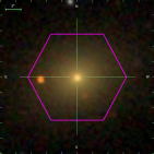
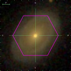
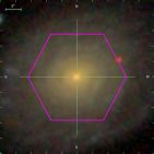
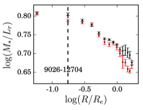
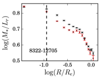
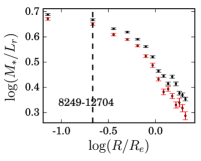
Figure 1: Fitting examples of an ETG (left column), a bulge+disk LTG (middle column), and a pure-disk LTG (right column). The top row shows the SDSS $gri$-bands stacked image for each galaxy with the MaNGA FoV overplotted as a pink hexagon. The bottom three panels show the corresponding radial $M_{*}/L_{r}$ variations of each galaxy, in which the black points with error bars are $(M_{*}/L_{r})_{\rm 2Dbin}$ with the values calculated from 2D maps, while those in red represent $(M_{*}/L_{r})_{\rm Rstack}$ with the values obtained from radially stacked spectra. In each bottom panel, the vertical dashed line shows the position of $1.5^{\prime\prime}$, which is the typical seeing of MaNGA observations.

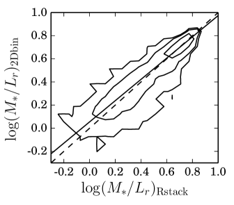
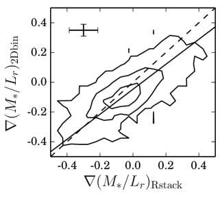
Figure 2: Comparison between two representations of $M_{*}/L_{r}$ and their radial gradients, with black contours showing the density distributions of Voronoi rebinned spectra in the left panel and galaxies in the right panel, respectively. Left panel: Corresponding to Figure 1, $\log(M_{*}/L_{r})_{\rm 2Dbin}$ are systematically higher than $\log(M_{*}/L_{r})_{\rm Rstack}$ at the low $M_{*}/L_{r}$ end, with the linear fitting result $\log(M_{*}/L_{r})_{\rm 2Dbin}=0.919\times\log(M_{*}/L_{r})_{\rm Rstack}-0.055$ as shown by the black solid line. Here we use the Python code LTS$\_$LINEFIT (Cappellari et al., 2013) for correlation analysis, the typical errors of $\log(M_{*}/L_{r})_{\rm 2Dbin}$ and $\log(M_{*}/L_{r})_{\rm Rstack}$ are roughly $\sim 0.01$. This correlation has Spearman correlation coefficient $r_{s}=0.91$ and Pearson correlation coefficient $r_{p}=0.9$. The linear slope $0.919\pm 0.004$ with a scatter of $0.061\pm 0.001$ is flatter than the dashed diagonal equality line. Right panel: The $M_{*}/L_{r}$ difference between the two methods causes a systematic bias to the measured $M_{*}/L_{r}$ gradients, with the linear fitting result $\nabla(M_{*}/L_{r})_{\rm 2Dbin}=0.840\times\nabla(M_{*}/L_{r})_{\rm Rstack}-0.047$ shown by the black solid line. The typical errors of $\nabla(M_{*}/L_{r})_{\rm Rstack}$ and $\nabla(M_{*}/L_{r})_{\rm 2Dbin}$ are displayed in the top-left of the right panel. This correlation has Spearman correlation coefficient $r_{s}=0.7$ and Pearson correlation coefficient $r_{p}=0.73$. The linear slope $0.840\pm 0.013$ with a scatter of $0.072\pm 0.004$ is flatter than the dashed diagonal equality line.

2.3 IFS data analysis

Since the surface brightness of a galaxy decreases with increasing radius, current MaNGA IFS observations can only provide an SDSS $r$-band, S/N$\sim 1$ per spectral pixel at the edge of their field of view (FoV). To improve the robustness of our stellar population analysis results, we first select those spaxels with S/N$>2$ and spatially rebin them to S/N$\sim 20$ using the Voronoi 2d binning method described in Cappellari & Copin (2003). There are 690,944 Voronoi bins in total obtained from the 2051 galaxies, with a median of 245 bins for each galaxy, and a median redshift of $z\sim 0.04$, which corresponds to 0.796 kpc/arcsec. For the total 690,944 spectra, $\sim 74\%$ of them have single pixels with $\rm S/N>20$, and only $\sim 3\%$ of them are rebinned from larger than 20 spaxels, which means the diameters of these bins are comparable to or larger than the spatial resolution of MaNGA observations (FWHM=2.5”, Bundy et al., 2015). When applying the Voronoi 2D binning method to improve the S/N of spaxels with $\rm S/N<20$, the basic assumption for those rebinned spaxels is that they have the same physical properties, since most of them ($\sim 97\%$) have the size smaller than the spatial resolution of MaNGA observation. For each Voronoi bin, we take the mean spectrum of all the stacked spaxels as the stacked spectrum, with the physical parameters of each spaxel in a spatial bin equal to each other.

After applying the pPXF code with our SSP libraries to these spatially rebinned spectra, by adopting 10th order multiplicative polynomials, we correct for inaccuracies in the spectral calibration and make the resulting data insensitive to reddening by dust (Cappellari, 2017). We then determine the stellar kinematic 2D distributions, which are used subsequently to correct galaxy rotation during the radial spectral stacking process.

To study galaxy’s $M_{*}/L$ gradient, we take the $M_{*}/L$ in the SDSS $r$-band for analysis, with the definition the same as in Equation (2) of Ge et al. (2018)

$$M_{*}/L_{r}=\frac{\Sigma f_{M,i}}{\Sigma f_{M,i}/(M_{*}/L_{r})_{i}}.$$ (1)

where $M_{*}$ of the $i$-th SSP template includes the mass in living stars and stellar remnants, but excludes the gas lost during stellar evolution. $(M_{*}/L_{r})_{i}$ corresponds to the $r$-band $M_{*}/L$ of the $i$-th template, and $f_{M,i}$ is the fitted mass fraction. The IFS spaxels of a galaxy are divided into different radial bins based on its ellipticity (or the $b/a$ axial ratio), position angle, and the brightest central spaxel in the SDSS $r-$band. Considering that the maximum MaNGA FoV of $\sim 30$ arcsec can cover the central 1.5$R_{e}$ for 60 per cent of galaxies and 2.5$R_{e}$ for 30 per cent of galaxies (Yan et al., 2016), we use the Python package MgeFit by Cappellari (2002) to model a galaxy’s surface brightness within its MaNGA FoV ($\leq 30$ arcsec). The MGE fitted $b/a$ axial ratio and position angle (rather than values for the whole galaxy) are used to construct radial bins for further spectral stacking or parameter estimations.

With interacting and barred galaxies excluded from our sample, the central brightest spaxel of each galaxy matches the luminosity-weighted galaxy centre well, and is therefore defined as the centre for bin construction. These bins are radial annuli formed by dividing the galaxy’s major axis into 1 arcsec intervals. Since the pixel size of MaNGA data is $0.5\times 0.5$ arcsec, each radial bin includes two spaxels in the major axis and at least one spaxel (for $b/a=0.5$) along the minor axis. For each galaxy, there are at most 15 concentric annuli for studying radial gradients in $M_{*}/L_{r}$ and the other stellar population parameters. Taking into account the typical seeing of FWHM $\sim 1.5$ arcsec for the MaNGA survey (Bundy et al., 2015), we only use those radial annuli whose radii measured along the major axis are larger than $1.5$ arcsec, and the number of annuli with observed spectra is at least 3 for gradient calculations. Considering that the MaNGA survey is designed for mapping nearby galaxies primarily to $1.5R_{e}$ (Yan et al., 2016), we set the cutoff of maximum radii to $1.5R_{e}$ for gradient fitting of each galaxy. The minimum radii of the elliptical bins are set to $0.1R_{e}$ or $1.5^{\prime\prime}$ for galaxies with low spatial resolution, by taking into account the typical seeing ($1.5^{\prime\prime}$) of MaNGA observations.

There are two ways of estimating parameters using the radial annuli: either use the median parameter values from individual spectra, or stack the spectra and then calculate the parameter values. For a particular elliptical bin, we can average each parameter based on all the spaxels included in the radial bin. For the second method, we also obtain the mean spectrum of all spaxels in this bin. Therefore, all quantities derived from the two methods can be comparable to each other. We explain and evaluate both methods, and compare the results obtained. In the first method, after the 2D Voronoi binning, we can perform pPXF fitting on the spectrum associated with each Voronoi bin, and calculate the stellar population parameter values, which can then be binned into the radial annuli. The radial distribution of each parameter (e.g. $(M_{*}/L_{r})_{\rm 2Dbin}$) can be obtained by calculating the median values in each annulus, with the scatter of each parameter being estimated as the root mean square value. In the second method, using the 2D velocity maps determined earlier (with rebinned spectral S/N$\sim 20$), we bring all the spectra in each radial annulus to the same velocity, i.e., $V_{*}=0$ km/s, and then stack them together. From these stacked spectra in each radial annulus, we can obtain (using pPXF again) the corresponding stellar population parameter values (e.g. $(M_{*}/L_{r})_{\rm Rstack}$).

Figure 1 shows three examples using both methods: an ETG, a bulge+disk LTG, and a pure-disk LTG. The bottom three panels show radial variations of $(M_{*}/L_{r})_{\rm 2Dbin}$ (black colour) and $(M_{*}/L_{r})_{\rm Rstack}$ (red colour), with the corresponding errors estimated in two different ways. The error bar of $(M_{*}/L_{r})_{\rm 2Dbin}$ is calculated based on all the spaxels in each annulus by assuming each spaxel has the same $M_{*}/L_{r}$ uncertainty. For $(M_{*}/L_{r})_{\rm Rstack}$, we obtain its uncertainty from its Monte-Carlo based estimation by assuming the flux error of stacked spectra obeys the standard normal distribution. For other surveys with higher spatial resolution, e.g., VLT/MUSE (Bacon et al., 2014), one can obtain more radial bins than the MaNGA case, which means more detailed substructures and possibly larger fluctuation appearing in the radial curve compared to MaNGA observations. As to the gradient fitting, the radial elliptical bins taken in our analysis are $2.5$ to $7.5$ times larger than the spatial resolution (FWHM) for the MaNGA primary galaxy sample (Table 3 of Bundy et al., 2015), which can already support a robust gradient measurement.

As shown in Figure 1, $(M_{*}/L_{r})_{\rm Rstack}<(M_{*}/L_{r})_{\rm 2Dbin}$ happens at different radii for different types of galaxies. ETGs have increasing differences with larger radii; bulge+disk LTGs have large differences for $\log(R/R_{e})\sim[-1.0,-0.2]$ and no significant difference at other radii; and pure-disk LTGs show a systematic decrease in $(M_{*}/L_{r})_{\rm Rstack}$ at all radii.

To have a thorough understanding on the difference between measured $(M_{*}/L_{r})_{\rm Rstack}$ and $(M_{*}/L_{r})_{\rm 2Dbin}$, we compare them directly in the left panel of Figure 2. By applying the Python code LTS$\_$LINEFIT in version 5.0.18 (Cappellari et al., 2013) for correlation analysis, the fitted slope of the correlation for the $\log(M_{*}/L_{r})_{\rm 2Dbin}$ vs. $\log(M_{*}/L_{r})_{\rm Rstack}$ plot is $0.919\pm 0.004$, which is flatter than the dashed diagonal equality line. At the high $M_{*}/L_{r}$ end, the values derived from the two methods are the same to each other, which indicates that for those old spectra without strong SFR, both the two methods can converge to the same results. With decreasing $M_{*}/L_{r}$, the bias of the $M_{*}/L_{r}$ measurements increase.

Bias in the two $M_{*}/L_{r}$ measurements also introduces a systematic bias to the slopes of radial $M_{*}/L_{r}$ gradients for galaxies in our sample as shown in the right panel of Figure 2. We find that $\nabla(M_{*}/L_{r})_{\rm 2Dbin}=0.84\times\nabla(M_{*}/L_{r})_{\rm Rstack}-0.05$, which is also derived using the Python code LTS$\_$LINEFIT. The fitted slope that is flatter than the diagonal equality line should be mainly caused by the spatially inhomogeneous surface densities of star formation rate (SFR) inside a galaxy. For spaxels in a radial annulus, if their SFRs have large variation, then those spaxels with higher SFRs can contribute a larger luminosity fraction than those with lower SFRs due to the larger luminosity fraction of young and high-mass stars. This makes the spectral fitting to the stacked spectrum biased to smaller $M_{*}/L$ since young stellar populations with higher luminosity can obscure signals from older ones, hence the derived $(M_{*}/L_{r})_{\rm Rstack}$ is smaller than the corresponding $(M_{*}/L_{r})_{\rm 2Dbin}$. To avoid the possible uncertainties caused by SFR variation, in this work, we take $(M_{*}/L_{r})_{\rm 2Dbin}$ instead of $(M_{*}/L_{r})_{\rm Rstack}$ for gradient and $M_{*}/L$-colour relation analyses.

The gradients are measured by performing a fit of the linear relation

$$\log(M_{*}/L_{r})=a+b\times\log(R/R_{e}).$$ (2)

within the radial range $0.1R_{e}$ (or 1.5 arcsec for low spatially resolved galaxies) and $1.5R_{e}$. We define the gradient as the slope of the linear fit $\nabla(M_{*}/L_{r})\equiv b$, and perform the fit using Numpy’s (Harris et al., 2020) polyfit. The formal errors are calculated from the returned covariance matrix. The gradients of other parameters including luminosity-weighted age $\log(t_{L}/\rm yr)$, mass-weighted age $\log(t_{M}/\rm yr)$, luminosity-weighted metallicity [M/H]_L, mass-weighted metallicity [M/H]_M, dust extinction E(B-V), and the star formation rate (SFR) and specific SFR in logarithms, i.e., $\log({\rm SFR})$ and $\log({\rm sSFR})$, are defined similarly. The errors in these gradients are estimated using the Python numpy (Oliphant, 2007) polyfit routine.

For each spatially rebinned spaxel, its SFR and sSFR are converted from the pPXF fitted $\rm H\alpha$ luminosity using the empirical law given by Kennicutt (1998) under the Salpeter IMF assumption,

$${\rm SFR}(M_{\odot}{\rm yr^{-1}})=7.9\times 10^{-42}L(\rm H\alpha)~{}(ergs~{}s^{-1}),$$ (3)

and the sSFR is defined as

$${\rm sSFR}~{}({\rm Gyr^{-1}})={\rm SFR}/M_{*}\times 10^{9}.$$ (4)

Given that the stellar age, metallicity, SFR, and sSFR of spaxels in ETGs and LTGs can actually cover several order of magnitudes, gradients are calculated logarithmically.

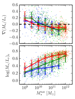
Figure 3: The logarithmic gradients of $M_{*}/L_{r}$ (top panel) defined in Equation (2) and the luminosity weighted mean values of $M_{*}/L_{r}$ inside one effective radius, i.e., $\log(M_{*}/L_{r})_{e}$ (bottom panel) as a function of galaxy stellar mass with different morphologies. The red, green, and blue points in each panel correspond to the ETGs, bulge+disk LTGs, and pure-disk LTGs, respectively. The median $M_{*}/L_{r}$ gradients in a set of mass bins for the three types of galaxies are also shown by open boxes with errors labelled in the same colours as the data points. The error bars indicate the 16th and 84th percentiles for each mass bin. The width of each mass bin is 0.5 dex. Only those mass bins with at least 3 galaxies inside are plotted. The dashed line in the top panel shows $\nabla(M_{*}/L_{r})=0$, which helps present when the median gradient reverts from positive to negative.

Figure 4: The averaged radial $M_{*}/L_{r}$ profiles for different galaxy types and mass bins corresponding to Figure 3. Panels from left to right show results for pure-disk LTGs, bulge+disk LTGs, and ETGs. Colours from dark blue to dark red represent the galaxy mass from $\log(M_{*}^{\rm tot}/M_{\odot})=9.0$ to $12.0$, as labelled in the left panel. By setting the galaxy radii ranging from 0.1 to 1.5 $R_{e}$ evenly sampled logrithmically, with each radial bin having a width of 0.1 dex, we calculate the averaged $\log(M_{*}/L_{r})$ and the corresponding uncertainty only if over 50% of galaxies included in this bin have been spatially resolved. Considering that the typical seeing of MaNGA observations is $1.5^{\prime\prime}$, the inner $\sim 3$ data points are mostly affected by the seeing effect than those outside radial bins.

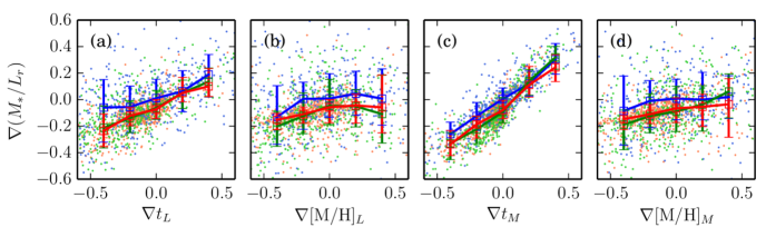
Figure 5: Correlations between $M_{*}/L_{r}$ gradients and other stellar population parameters: gradients of luminosity-weighted stellar age ($t_{L}$, panel a), luminosity-weighted stellar metallicity ([M/H]_L, panel b), mass-weighted stellar age ($t_{M}$, panel c), and mass-weighted stellar metallicity ([M/H]_M, panel d). ETGs, LTGs with and without a central bulge are shown in red, green, and blue colours, respectively. The median values in each age or metallicity gradient bins are shown by open boxes and the associated error bars (16th and 84th percentiles) in the same colour correspondingly.

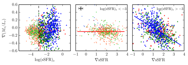
Figure 6: The $M_{*}/L_{r}$ gradients as a function of sSFR inside a galaxy’s half light radius $\log({\rm sSFR})_{e}$ (left panel) and $\nabla{\rm sSFR}$ for $\log({\rm sSFR})_{e}<-3$ (middle panel) and $\log({\rm sSFR})_{e}>-3$ (right panel) cases. The red, green, and blue points correspond to the ETGs, bulge+disk LTGs, and pure-disk LTGs, respectively. The vertical dashed line in the left panel shows the criterion of $\log({\rm sSFR})_{e}=-3$. Here we especially label those galaxies with $\log({\rm sSFR})_{e}>-3$ by triangles in the corresponding darker colours. In the middle panel, galaxies with $\log({\rm sSFR})_{e}<-3$ are plotted to present the $\nabla(M_{*}/L_{r})$ as a function of $\nabla{\rm sSFR}$, and a linear fitting of these points are shown in red solid line with a slope of 0.0. The top-left horizontal and vertical error bars show the median errors of $\nabla{\rm sSFR}$ and $\nabla(M_{*}/L_{r})$ of the galaxy sample, respectively. The right panel plots those galaxies with $\log({\rm sSFR})_{e}>-3$, and has the linear fitting result overlapped as a blue solid line with a slope of $-0.167\pm 0.009$ and scatter of $0.172\pm 0.005$ obtained from the LTS$\_$LINEFIT correlation analysis.

Figure 7: Galaxy properties as a function of stellar mass. Panels from (a) to (h) show $\nabla t_{L}$, $\nabla{\rm[M/H]}_{L}$, $\nabla t_{M}$, $\nabla{\rm[M/H]}_{M}$, $\log({\rm sSFR})_{e}$, $\nabla{\rm E(B-V)}$, $\nabla{\rm SFR}$, and $\nabla{\rm sSFR}$ in terms of the galaxy stellar mass $M_{*}^{\rm tot}=2\times M_{*}^{e}$. As shown in Figure 3, the red, green, and blue points, and also the corresponding median value with error bars represented by 16th and 84th percentiles show the results of ETGs, LTGs with and without bulges, respectively.

3 Results

We first study the properties of $M_{*}/L_{r}$ gradients using a radially fixed Salpeter IMF assumption for galaxies with different morphologies. The results could help understand the evolution of different galaxy types and their resulting gradient distributions. We then introduce radially varying IMFs and consider their impact on the gradients and the relations between $M_{*}/L_{r}$ and galaxy colours.

3.1 $M_{*}/L_{r}$ gradients for galaxies with different morphologies and the fixed Salpeter IMF assumption

The top panel of Figure 3 shows the $M_{*}/L_{r}$ gradients as a function of stellar mass for three kinds of galaxies: ETGs (red points), bulge+disk LTGs (green points), and pure-disk LTGs (blue points). Here the galaxy stellar mass is estimated by

$$M_{*}^{\rm tot}=(M_{*}/L_{r})_{e}\times L_{r}^{\rm tot},$$ (5)

where $(M_{*}/L_{r})_{e}$ is the projected stellar mass to light ratio inside the half light radius $R_{e}$ under the assumption of a constant Salpeter IMF, which is calculated based on the 2D $M_{*}/L_{r}$ maps and the corresponding $r$-band luminosity

$$(M_{*}/L_{r})_{e}=\frac{\sum_{j=1}^{N}L_{r,j}(M_{*}/L_{r})_{j}}{\sum_{j=1}^{N}L_{r,j}}.$$ (6)

where $N$ is the total number of spaxels inside $R_{e}$, and $L_{r,j}$ and $(M_{*}/L_{r})_{j}$ are the $r$-band luminosity and $M_{*}/L_{r}$ of the $j$th spaxel, respectively.

This estimate assumes that the $(M_{*}/L_{r})_{e}$ is representative of the one over the full galaxy, and a better estimate could be obtained if we could directly measure the $M_{*}/L$ over the full galaxy. However, the MaNGA survey is limited to 1.5$R_{e}$ for most galaxies (Bundy et al., 2015; Yan et al., 2016), we can not derive the whole 2D mass distribution by only using MaNGA data. As shown in the top panel, massive galaxies with total stellar mass larger than $10^{11}M_{\odot}$ have negative gradients with median values in the range [-0.2,-0.15], which is consistent with results from Szomoru et al. (2013), Newman, Ellis, & Treu (2015), Li et al. (2018), and Sonnenfeld et al. (2018). In particular, Li et al. (2018) used the same approach and MaNGA data but with a different galaxy sample, and our results are consistent with each other. The gradients become shallower with lower stellar mass for galaxies with $M_{*}^{\rm tot}\leq 10^{10}M_{\odot}$, and this trend is similar to that found in Tortora et al. (2011). For the $\nabla(M_{*}/L_{r})$-mass correlations, all three types of galaxies show no significant difference. Whether pure-disk LTGs have a similar formation scenario as elliptical and bulge-dominated galaxies requires further exploration.

The difference between ETGs and bulge+disk LTGs is reflected by the luminosity weighted mean $M_{*}/L_{r}$ inside the galaxy half light radius $\log(M_{*}/L_{r})_{e}$ versus galaxy stellar mass plot shown in the bottom panel of Figure 3. This correlation is similar to that of $\log(M_{*}/L_{r})_{e}$ versus velocity dispersion as shown Figure 5 of Li et al. (2018). With increasing galaxy stellar mass or velocity dispersion, galaxies tend to have higher $M_{*}/L_{r}$, in which ETGs have the largest values, pure-disk LTGs have the smallest, while those of bulge+disk LTGs lie in between.

Figure 4 presents another way of analyzing the radial $M_{*}/L_{r}$ profiles, by using the averaged radial $M_{*}/L_{r}$ profiles for the three kinds of galaxies at different mass bins to study their evolution trends. With increasing stellar mass, the slopes of those radial profiles are positive for low mass bins and become negative for massive bins, presenting similar trends as shown in the top panel of Figure 3. At the same time, the averaged $M_{*}/L_{r}$ in each mass bin also increase with increasing galaxy mass, which is consistent with the bottom panel of Figure 3.

To explore the evolution details of these galaxies, we first show $\nabla M_{*}/L_{r}$ as a function of age and metallicity gradients in both the luminosity- and mass-weighted cases in Figure 5. Since the $M_{*}/L$ of a spectrum is mainly determined by its stellar age, as a natural consequence, $\nabla M_{*}/L_{r}$ correlates tightest with the age gradient (panels a and c) rather than the metallicity gradient as shown in panels (b) and (d). The $M_{*}/L_{r}$ gradients correlate with the mass-weighted stellar age gradients (panel c) more tightly than the luminosity-weighted ones (panel a). For all three kinds of galaxies, their $\nabla M_{*}/L_{r}$ increases with the stellar mass-weighted age gradient $\nabla t_{M}$ in a consistent way and the trends are close to the diagonal line (panel c). For the luminosity-weighted case (panel a), the $\nabla M_{*}/L_{r}$ vs. the luminosity-weighted age gradient $\nabla(t_{L})$ trends are largely biased away from the diagonal line, with pure-disk LTGs have the larger biases than ETGs and bulge+disk LTGs. This could be caused by stronger star formation happening in pure-disk LTGs than the other two kinds of galaxies.

At a certain stellar age, stellar spectra with larger metallicities also have higher $M_{*}/L_{r}$ (e.g. Figure 2 of Ge et al., 2019). This also explains the positive correlation between $\nabla M_{*}/L_{r}$ and metallicity gradient $\nabla{\rm[M/H]}$, which is clearly weaker than that between the $\nabla M_{*}/L_{r}$ and $\nabla t$, as shown in panels (b) and (d) of Figure 5. Compared to the monotonically increasing trend in the mass-weighted case shown in panel (d), the weakly increasing trend for $\nabla M_{*}/L_{r}$ as a function of $\nabla{\rm[M/H]}_{L}$ (panel b) becomes flat for bulge+disk LTGs and even inverts for pure-disk LTGs when $\nabla{\rm[M/H]}_{L}>0$. Again, this might also be caused by different star formation strengths.

Since star formation can affect the $\nabla(M_{*}/L_{r})$ estimates, Figure 6 is plotted showing the variation in galaxy sSFR with $\nabla(M_{*}/L_{r})$. Galaxies with $({\rm sSFR})_{e}<10^{-3}{\rm Gyr}^{-1}$ (solid circles in the left panel) can be classified by the origin of H$\alpha$ emission lines, with ionization not only from SFR, but also hot low-mass evolved stars and weak active galactic nuclei (AGNs, e.g. Stasińska et al., 2008; Cid Fernandes et al., 2011). From the WHAN diagram of Cid Fernandes et al. (2011), passive galaxies and LINER dominate the weak emission line systems, which means that galaxies in the middle panel of Figure 6 are dominated by these two kinds of objects. H$\alpha$ emission lines ionized by hot low-mass evolved stars and weak AGNs would not support a strong correlation between sSFR and $M_{*}/L_{r}$ gradients. These passive galaxies with weak SFR have little effect on the $\nabla M_{*}/L_{r}$ estimates. Hence we obtain a slope of zero (red line in the middle panel) of their correlations. For star-forming galaxies with $({\rm sSFR})_{e}>10^{-3}{\rm Gyr}^{-1}$, a clear anti-correlation between $\nabla{\rm sSFR}$ and $\nabla M_{*}/L_{r}$ appears (blue line in the right panel). By performing the linear correlation analysis with LTS$\_$LINEFIT, we determine that this anti-correlation has a slope of $-0.167\pm 0.009$ with a scatter of $0.172\pm 0.005$. The two kinds of correlation behaviours indicate that star formation in passive galaxies contributes little to the measurements of stellar ages and $M_{*}/L_{r}$. However, for star-forming galaxies, a higher sSFR can produce a younger luminosity-weighted age and hence smaller $M_{*}/L_{r}$. This means that for a galaxy with a positive sSFR gradient and $({\rm sSFR})_{e}>10^{-3}{\rm Gyr}^{-1}$, the galaxy tends to have a more negative $\nabla t_{L}$ and $\nabla(M_{*}/L_{r})$. Therefore, the anti-correlation shown in the right panel of Figure 6 explains why the $\nabla(M_{*}/L_{r})$ as a function of $\nabla t_{L}$ presents different trends from that of $\nabla t_{M}$ as shown in panels (a) and (c) of Figure 5, respectively.

According to the results shown in the bottom panel of Figure 3, bulge+disk LTGs lie between the ETGs and pure-disk LTGs. In the middle and right panels of Figure 6, galaxies with different ${\rm sSFR}_{e}$ have their $\nabla(M_{*}/L_{r})$ and $\nabla{\rm sSFR}$ correlated in two ways. To understand further how ETGs and LTGs evolve with their mass, we explore the stellar population gradients in terms of their total stellar mass $M_{*}^{\rm tot}$.

As shown in Figure 7, both the luminosity-weighted ($\nabla t_{L}$, panel a) and mass-weighted ($\nabla t_{M}$, panel c) age gradients show similar trends with increasing stellar mass as $\nabla(M_{*}/L_{r})$ (top panel of Figure 3), because of their positive correlations as presented in panels (a) and (c) of Figure 5. The $\nabla{\rm[M/H]}_{L}$ (panel b) and $\nabla{\rm[M/H]}_{M}$ (panel d) show a systematic decreasing trend with increasing galaxy mass, although with a large scatter when taking the 16th and 84th percentiles as error bars. ETGs, with the largest $(M_{*}/L_{r})_{e}$ (bottom panel of Figure 3), tend to have lower sSFR than LTGs, and pure-disk LTGs have the largest sSFR in each mass bin, with bulge+disk LTGs lying in between (panel e). The median values of $\nabla\rm E(B-V)$ (panel f) and $\nabla\rm SFR$ (panel g) are consistent with each other and fluctuate around zero. The $\nabla\rm SFR$ distributions have larger scatters than that of the E(B-V) gradients, especially for ETGs and bulge+disk LTGs. Even though we have improved the spectra S/N by spatially stacking spectra, this step mainly improves the robustness of E(B-V) estimates resulting from stellar population analysis. The H$\alpha$ emission lines are still weak compared to the continua due to the lower SFR of ETGs and bulge-dominant LTGs, hence H$\alpha$-based $\nabla\rm SFR$ values show larger scatter than that of $\nabla\rm E(B-V)$. The age, metallicity, and $M_{*}/L_{r}$ gradients have weakly decreasing trends with increasing galaxy mass. This can be explained by the correspondingly increased sSFR gradients as shown in panel (h).

3.2 $M_{*}/L_{r}$-colour relations

For galaxies in our sample, we take the $M_{*}/L_{r}$ values for all the spatially rebinned spaxels, and use them to investigate potential relationships between $M_{*}/L_{r}$ and colours. Here we take $g-r$, $r-i$, and $g-i$ colours from the SDSS $gri$ bands for analyses. By applying the pPXF fitted E(B-V) dust extinction correction to the $gri$ band luminosities, all three colours are dust extinction corrected.

Figure 8: The $M_{*}/L_{r}$ and colour relations after assuming a universal Salpeter IMF. Panels from left to right correspond to the correlations with SDSS $g-r$, $r-i$, and $g-i$ colours, with all the colours are dust extinction corrected based on the fitted E(B-V) in pPXF fitting. In each panel, the black contours show the density distribution of pixels with number density larger than 10, which means that all the pixels shown here have S/N$>3$ in the case of poisson noise distribution. We fit the correlation by $\log(M_{*}/L_{r})=a+b\times{\rm colour}$, and show the fitting result as the black solid lines. Those pixels with colours from blue to red represent the mean luminosity-weighted (top three panels) or mass-weighted (middle three panels) stellar ages from young to old. In the middle three panels, the black dashed lines show linear fitting results of those spectra with mass-weighted stellar age $t_{M}>10$ Gyr. In the bottom three panels, we present the age difference between the mass- and luminosity-weighted stellar ages, i.e., $\Delta\log t=\log(t_{M}/t_{L})$. Blue colours indicate SFHs dominated by a single burst while redder colours correspond to more complex SFHs with higher fraction of newly formed stars.

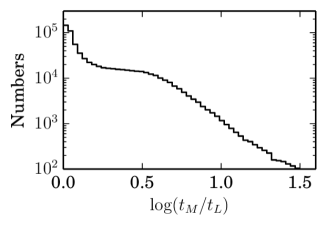
Figure 9: Number distribution of $\Delta\log t=\log(t_{M}/t_{L})$ for 690,944 spectra from the Voronoi 2D binning of 2051 galaxies, in which 111,613 spectra ($\sim 16\%$) have $\Delta\log t>0.5$, and 6,777 spectra ($\sim 1\%$) have $\Delta\log t>1.0$.

Table 1: The $M_{*}/L_{r}$ as a function of colour at fixed Salpeter IMF assumption

colour	$a$	$b$	$a_{\rm o}$	$b_{\rm o}$
$g-r$	0.20	0.87	0.47	0.45
$r-i$	0.37	2.10	0.55	1.12
$g-i$	0.24	0.63	0.48	0.33

Note: For the fitting function of $\log(M_{*}/L_{r})=a+b\times{\rm colour}$. The subscript $\rm o$ represents the fitting results of those spectra with older mass-weighted stellar ages ($t_{M}>10$ Gyr).

Figure 8 shows $M_{*}/L_{r}$ as a function of SDSS $g-r$ (left column), $r-i$ (middle column), and $g-i$ colours (right column) under the assumption of a universal Salpeter IMF. The dashed line in each panel shows the linear fitting result of the $M_{*}/L_{r}$-colour correlation, with the detailed parameters listed in Table 1. In each panel, we can see a tight linear correlation (e.g. Bell & de Jong, 2001) for $\sim 80$ per cent of spaxels (surrounded by the first and second central contours). Other works (e.g. García-Benito et al., 2019), find a similar result. Compared to Bell & de Jong (2001), which studied the $M_{*}/L$-colour relations by assuming different galaxy evolution models, our results provide the statistical $M_{*}/L$-colour correlation coefficients of galaxies with real SFHs at redshift range $z\sim[0,0.15]$ (Bundy et al., 2015). Spectra from IFS observations with the FoV covering $\geq 1.5R_{e}$ also contain more complex SFHs than single observed spectra only focusing on the central 3 arcsec diameter fibre (e.g. Bell et al., 2003). Therefore, the correlation coefficients of $M_{*}/L_{r}$ vs. $g-r,r-i$, and $g-i$ colour relations vary slightly but are roughly consistent with that of Bell et al. (2003).

$M_{*}/L_{r}$ not only correlates well with galaxy colours, but also with luminosity-weighted stellar ages ($t_{L}$, see the top three panels of Figure 8). However, for the mass-weighted stellar age ($t_{M}$) case (the middle row of Figure 8), the correlation behaviours among them are different from that of the $t_{L}$ case. Spaxels with similar $t_{M}$ can have different colours. This is due to the varied star formation histories that have occurred (e.g. Bell et al., 2003; Gallazzi & Bell, 2009). As studied in Yesuf et al. (2014) and Pawlik et al. (2018), post-starburst galaxies can be divided into several types based on the fraction and appearence time of starbursts in the star formation history (SFH). In the bottom row of Figure 8, we plot the age difference of each spectrum $\Delta\log t=\log(t_{M}/t_{L})$ as an indicator for reflecting the contribution of newly formed stars to the whole SFH. For example, post starburst galaxies with their recent star bursts happening in the last 1 Gyr can change the galaxy colours from red to blue, but the $t_{M}$ can still be $\sim 10$ Gyr, and is largely biased from an exponential SFH. In the bottom panels of Figure 8, those pixels in red show galaxies with SFHs having the strongest recent starbursts. Spaxels with similar SFHs as post-starburst galaxies can lie on the top-left of the density distribution in each panel, i.e., spaxels with a little bit smaller $M_{*}/L_{r}$, $t_{M}\sim 10$ Gyr, and blue colours, as shown in the middle row of Figure 8. However, their age differences are larger than those with the same $M_{*}/L_{r}$ with redder galaxy colours, or the same galaxy colours with lower $M_{*}/L_{r}$.

Those spaxels with large age difference are not insignificant for the current sample. Figure 9 shows the $\Delta\log t$ distribution for all rebinned spectra of our galaxy sample, in which $\sim 16\%$ of the total spaxels have $\Delta\log t>0.5$ dex, and $\sim 5\%$ of them have $\Delta\log t>1.0$ dex, which means that their newly formed stars can have a significant effect on changing of spectral shape and galaxy colours.

The correlation coefficients of those spaxels with stellar age older than 10 Gyr are also listed in Table 1, and are systematically flattened compared to all spaxels. A similar result is found by Gallazzi & Bell (2009) (see their Figure 11), which has less complex SFHs assumed than the observed MaNGA data. Our results actually complement the missing top-left part in their Figure 11 that has blue colours but old populations with high $M_{*}/L_{r}$.

With the statistical analyses on the effect of complex SFHs to the $M_{*}/L_{r}$-galaxy colour relations, the correlation slopes obtained by different works are mainly determined by their galaxy types. For local galaxies, the slopes obtained in different works are no flatter than the $b_{\rm o}$ listed in Table 1, but the detailed values could vary due to the different selection criteria of their galaxy samples, which indicates that varied SFH distributions are covered in the $M_{*}/L$-colour relations (e.g. Bell & de Jong, 2001; Bell et al., 2003; Gallazzi & Bell, 2009; García-Benito et al., 2019).

4 Discussion

4.1 Comparison with previous works

Tortora et al. (2011) performed SED fitting of SDSS $ugriz$ bands for 50,000 galaxies and found that galaxies of different types show different behaviours for their $M_{*}/L$ gradients as a function of stellar mass. For LTGs, gradients steepen negatively with increasing mass, while for ETGs, gradients first decrease with increasing mass up to $\sim 10^{10.3}M_{\odot}$, and then increase with increasing mass. The advantage of using photometric data with stellar population analysis is that galaxy images can be obtained with much less observation time and higher S/N and larger FoV than that for IFU observations. However, the fitted results are contaminated by both emission line (e.g. H$\alpha$) contributions to different bands (especially for LTGs), and lack of absorption lines, which introduces large uncertainties caused by the degeneracy between age, metallicity, and dust extinction.

Compared to the results obtained from SED fittings (Tortora et al., 2011), MaNGA data provide us with spectral resolution ($R\sim 2000$, Smee et al., 2013) high enough to resolve absorption lines and with wide enough spectral wavelength coverage (3600-10500Å, Bundy et al., 2015) to perform reliable stellar population analyses, if we choose a suitable spectral fitting code and SSP library. For the pPXF code used in this work, the dust extinction uncertainty is less than 0.01 mag for galaxy spectra with age $t>0.1$ Gyr, as shown in Figure 4 of Ge et al. (2018). This indicates that the degeneracy between stellar age and dust extinction in the SED fitting process cannot contaminate our analyses of MaNGA data if the assumed dust reddening curve is precise enough. However, many efforts focusing on the dust reddening curve show that the dust-star geometry is complex and that star-forming regions even require a two-component dust model for explanation (e.g. Charlot & Fall, 2000; Wilkinson et al., 2015, 2017; Li et al., 2020, 2021).

The sample size of Tortora et al. (2011) is, however, larger than the number of galaxies selected in our work, and their galaxies are fainter than ours. The photometrically selected galaxy sample can have galaxy stellar masses ranging from $10^{7.7}M_{\odot}$ to the most massive galaxies (see their Figure 3 for details) in the SDSS photometric survey. The current MaNGA survey has smaller mass coverage (see Figure 3) than in the Tortora sample.

4.2 Previous usage of M/L gradients in dynamical models

In external galaxy dynamical modelling, e.g., Jeans equations modelling (Cappellari, 2008), orbit based modelling (Schwarzschild, 1979), or particle-based modelling (Syer & Tremaine, 1996) in the past it was common to adopt mass-follow-light models assuming a constant $M_{*}/L$ (e.g. van der Marel, 1991; Cappellari et al., 2006; Long & Mao, 2012). It was motivated by simplicity and by the fact that the dynamical models were targeting central parts of early-type galaxies, where population gradients are modest.

Some papers assessed the influence of $M_{*}/L$ gradients on masses of supermassive black holes (e.g. Cappellari et al., 2002; McConnell et al., 2013; Thater et al., 2017, 2019). They found that ignoring $M_{*}/L$ variations in mass-follow-light models can lead to biases in the black hole masses.

However, one fact that is not always appreciated is that the stellar surface brightness (as opposed to the stellar mass density) remains the best approximation for the stellar-tracer population, even when $M_{*}/L$ gradients are present. It implies that one can still correctly model the galaxies’ total density, without distinguishing what fraction is due to the stellar mass and which one is due to the dark matter. In this case, one treats the stars only as a tracer population orbiting in the total gravitational potential and recovers reliable total densities without the need to know the $M_{*}/L$ gradients (e.g. Cappellari et al., 2015; Poci et al., 2017; Mitzkus et al., 2017).

On the other hand, focusing on the total density alone, in the presence of significant $M_{*}/L$ gradients, prevents one from measuring unbiased dark matter profiles or estimating the stellar $M_{*}/L$ (and IMF). For this, one has to explicitly include the $M_{*}/L$ gradients in the mass models as done in more recent studies based on IFS data (Mitzkus et al., 2017; Poci et al., 2017; Li et al., 2017). In this situation, our assessment of systematic trends of $M_{*}/L$ gradients in galaxies becomes relevant.

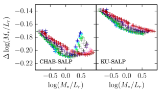
Figure 10: The $M_{*}/L_{r}$ differences ($\Delta(M_{*}/L_{r})$) as a function of $M_{*}/L_{r}$ in the Salpeter IMF for the Vazdekis/MILES model based SSP libraries. The left panel shows the $\Delta(M_{*}/L_{r})$ between the Chabrier and Salpeter IMFs (i.e. CHAB$-$SALP), while the right panel presents that between Kroupa Universal and Salpeter IMFs (i.e. KU$-$SALP). In each panel, the 12 kinds of stellar metallicities from poor ([M/H]$=-2.27$) to rich ($0.4$) are labelled with colours from blue to red, respectively.

4.3 Effect of radial IMF variations to $\nabla M_{*}/L$ measurements

Once a galaxy has radially varying IMFs (see a review by Smith, 2020), then the $M_{*}/L$ gradients will become more negative than the constant IMF case as assumed in this work. Figure 10 shows the $M_{*}/L_{r}$ difference between the Salpeter and Chabrier (or Kroupa) IMFs in the left (or right) panel, which means that, if we assume a galaxy has a Salpeter IMF at $0.1R_{e}$ and a Chabrier (or Kroupa) IMF at $1R_{e}$, the corresponding $M_{*}/L_{r}$ difference shown in the left (or right) panel is exactly the $M_{*}/L_{r}$ gradient that is further steepened (see detailed discussion in García-Benito et al., 2019).

If $M_{*}/L$-colour relations are applied to convert the galaxy colours to $M_{*}/L$, the correlation slopes are also steepened by potential radial IMF variations, leading to another difference with a constant $M_{*}/L$ approach. For example, Li et al. (2020) in modelling M87 utilized a $M_{*}/L$ profile produced by Sarzi et al. (2018), which revealed a strong negative IMF gradient by taking the IMF-sensitive absorption line features for stellar population analyses, and caused over a factor 2 increase in $M_{*}/L$ compared to the case of a Milky Way IMF.

5 Conclusions

Using a sample of 2051 face-on galaxies selected from the MaNGA sample released in SDSS DR15, we have investigated how galaxy $M_{*}/L_{r}$ gradients depend on morphology under the assumption of a universal Salpeter IMF. We exclude galaxies that are merging, barred, highly inclined ($i>45^{\circ}$), or have insufficient S/N to ensure robust stellar population analyses for calculations of stellar population gradients. We classify our galaxies into three groups: 1) ETGs, 2) LTGs with both bulge and disk components (bulge+disk LTGs), and 3) LTGs only having one disk component (pure-disk LTGs).

The $M_{*}/L_{r}$ gradients for all the three types of galaxies have similar trends as a function of galaxy stellar mass, i.e., $\nabla(M_{*}/L_{r})$ reverts from positive ($\sim 0.1$) to negative ($\sim-0.1$) when galaxy masses increasing from the lowest ($\sim 10^{9}M_{\odot}$) to the highest ones ($\sim 10^{12}M_{\odot}$). With increasing galaxy stellar mass, the luminosity weighted $M_{*}/L_{r}$ inside a half light radius $\log(M_{*}/L_{r})_{e}$ also increases, with the trends similar to that found in the velocity dispersion $\sigma_{e}$ vs. $\log(M_{*}/L_{r})_{e}$ correlations (e.g. Li et al., 2018). The age gradients as a function of $M_{*}^{\rm tot}$ show similar trend as $\nabla M_{*}/L_{r}$, while the metallicity gradients systematically decrease with increasing $M_{*}^{\rm tot}$. For $\log(M_{*}/L_{r})_{e}$ in different mass bin, ETGs have the largest values, and pure-disk LTGs have the smallest, while bulge+disk LTGs lie in between. Correspondingly, the sSFR inside $1R_{e}$ (sSFR_e) is the lowest for ETGs, and the highest for pure-disk LTGs.

$\nabla(M_{*}/L_{r})$ correlates with mass-weighted stellar age gradients ($\nabla t_{M}$) more so than other parameters. Its correlation with luminosity-weighted age gradients ($\nabla t_{L}$) is significantly affected by the star formation when ${\rm sSFR}_{e}$ is greater than $10^{-3}{\rm Gyr}^{-1}$, where these galaxies have their $\nabla(M_{*}/L_{r})$ decreasing with increasing $\nabla{\rm sSFR}$. This indicates that a stronger sSFR in the outer radii leads to smaller $t_{L}$ and $M_{*}/L_{r}$, and hence more negative $\nabla t_{L}$ and $\nabla(M_{*}/L_{r})$. The weak positive correlations between $\nabla(M_{*}/L_{r})$ and metallicity gradients are also affected by the galaxy star formation rate.

For the $M_{*}/L_{r}$-colour relations, old populations with stellar age older than 10 Gyr tend to have shallower correlation slopes than the global ones. In particular, the conversion of $M_{*}/L$ from galaxy colours for post starburst galaxies should be very carefully calculated when their SFHs include old populations dominating the stellar mass but newly formed stars dominating the luminosity.

Data availability

The data underlying this article will be shared on reasonable request to the corresponding author.

References

- Aguado et al. (2019) Aguado, D. S., Ahumada, R., Almeida, A., et al. 2019, ApJS, 240, 23
- Alton, Smith & Lucey (2018) Alton, P. D., Smith, R. J. & Lucey, J. R. 2018, MNRAS, 478, 4464
- Auger et al. (2010) Auger, M. W., Treu, T., Gavazzi, R., et al. 2010, ApJ, 721, L163
- Bacon et al. (2014) Bacon, R., Vernet, J., Borisova, E., et al. 2014, The Messenger, 157, 13
- Bell & de Jong (2001) Bell, E.F., de Jong R. S. 2001, ApJ, 550, 212
- Bell et al. (2003) Bell, E. F. et al. 2003, ApJS, 149, 289
- Bezanson et al. (2009) Bezanson, R., van Dokkum, P. G., Tal, T. et al. 2009, ApJ, 697, 1290
- Bundy et al. (2015) Bundy, K., Bershady, M. A., Law, D. R. et al. 2015, ApJ, 798, 7
- Calzetti et al. (2000) Calzetti, D., Armus, L., Bohlin, R. C. et al. 2000, ApJ, 533, 682
- Cappellari (2002) Cappellari, M. 2002, MNRAS, 333, 400
- Cappellari et al. (2002) Cappellari, M., Verolme, E. K., van der Marel, R. P., et al. 2002, ApJ, 578, 787
- Cappellari & Copin (2003) Cappellari, M. & Copin, Y. 2003, MNRAS, 342, 345
- Cappellari & Emsellem (2004) Cappellari, M. & Emsellem, E. 2004, PASP, 116, 138
- Cappellari et al. (2006) Cappellari, M., Bacon, R., Bureau, M., et al. 2006, MNRAS, 366, 1126
- Cappellari (2008) Cappellari, M. 2008, MNRAS, 390, 71
- Cappellari et al. (2012) Cappellari, M., McDermid, R. M., Alatalo, K. et al. 2012, Nature, 484, 485
- Cappellari et al. (2013) Cappellari, M., Scott, N., Alatalo, K., et al. 2013, MNRAS, 432, 1709
- Cappellari et al. (2015) Cappellari, M., Romanowsky, A. J., Brodie, J. P., et al. 2015, ApJ, 804, L21
- Cappellari (2016) Cappellari, M., 2016, ARA&A, 54, 597
- Cappellari (2017) Cappellari, M., 2017, MNRAS, 466, 798
- Chabrier (2003) Chabrier, G. 2003, PASP, 115, 763
- Charlot & Fall (2000) Charlot, S. & Fall, S. M. 2000, ApJ, 539, 718
- Cid Fernandes et al. (2011) Cid Fernandes, R., Stasińska, G., Mateus, A., et al. 2011, MNRAS, 413, 1687
- Ciotti et al. (2007) Ciotti, L., Lanzoni, B., & Volonteri, M. 2007, ApJ, 658, 65
- Conroy (2013) Conroy, C. 2013, ARA&A, 51, 393
- Conroy et al. (2017) Conroy, C., van Dokkum, P. G. & Villaume, A. 2017, ApJ, 837, 166
- Cordier et al. (2007) Cordier, D., Pietrinferni, A., Cassisi, S., Salaris, M. 2007, AJ, 133, 468
- Domínguez Sánchez et al. (2018) Domínguez Sánchez, H., Huertas-Company, M., Bernardi, M., Tuccillo, D., & Fischer, J. L. 2018, MNRAS, 476, 3661
- Domínguez Sánchez et al. (2019) Domínguez Sánchez, H., Bernardi, M., Brownstein, J. R., et al. 2019, MNRAS, 489, 5612
- Du et al. (2019) Du, C., Li, N., & Li, C. 2019, RAA, 12, 171
- Eggen et al. (1962) Eggen, O.J., Lynden-Bell, D., & Sandage, A. R. 1962, ApJ, 136, 748
- Ferreras et al. (2013) Ferreras, I., La Barbera, F., de la Rosa, I. G., et al. 2013, MNRAS, 429, L15
- Fischer et al. (2019) Fischer, J.-L., Domínguez Sánchez, H., & Bernardi, M. 2019, MNRAS, 483, 2057
- García-Benito et al. (2019) García-Benito, R., González Delgado, R. M., Pérez, E., et al. 2019, A&A, 621, A120
- Ge et al. (2018) Ge, J., Yan, R., Cappellari, M. et al. 2018, MNRAS, 478, 2633
- Ge et al. (2019) Ge, J., Mao, S., Lu, Y. et al. 2019, MNRAS, 485, 1675
- Gallazzi & Bell (2009) Gallazzi, A. & Bell, E. F. 2009, ApJS, 185, 253
- Goddard et al. (2017) Goddard, D. et al., 2017, MNRAS, 466, 4731
- González Delgado et al. (2015) González Delgado, R. M., García-Benito, R., Pérez, E., et al. 2015, A&A, 581, A103
- Harris et al. (2020) Harris, C.R., Millman, K.J., van der Walt, S.J. et al. 2020, Nature, 585, 357
- Hopkins et al. (2009) Hopkins, P. F., Bundy, K., Murray, N. et al. 2009, MNRAS, 398, 898
- Hopkins et al. (2010) Hopkins, P. F., Bundy, K., Hernquist, L. et al. 2010, MNRAS, 401, 1099
- Kennicutt (1998) Kennicutt, R. C. 1998, ARA&A, 36, 189
- Koleva et al. (2011) Koleva, M., Prugniel, P., De Rijcke, S., et al. 2011, MNRAS, 417, 1643
- Kroupa (2001) Kroupa, P. 2001, MNRAS, 322, 231
- Kuntschner et al. (2010) Kuntschner, H., Emsellem, E., Bacon, R., et al. 2010, MNRAS, 408, 97
- Larson (1974) Larson, R. B. 1974, MNRAS, 166, 585
- Li et al. (2020) Li, C., Zhu, L., Long, R. J., et al. 2020, MNRAS, 492, 2775
- Li et al. (2017) Li, H., Ge, J., Mao, S., et al. 2017, ApJ, 838, 77
- Li et al. (2018) Li, H., Mao, S., Cappellari, M., et al. 2018, MNRAS, 476, 1765
- Li et al. (2020) Li, N., Li, C., Mo, H., et al. 2020, ApJ, 896, 38
- Li et al. (2021) Li, N., Li, C., Mo, H., et al. 2021, arXiv:2103.00666
- Long & Mao (2012) Long, R. J. & Mao, S. 2012, MNRAS, 421, 2580
- Lu et al. (2020) Lu, S., Cappellari, M., Mao, S., et al. 2020, MNRAS, 495, 4820
- McConnell et al. (2013) McConnell, N. J., Chen, S.-F. S., Ma, C.-P., et al. 2013, ApJ, 768, L21
- Martin-Navarro et al. (2018) Martin-Navarro, I., Vazdekis, A., Falcon-Barroso, J. et al. 2018, MNRAS, 475, 3700
- Mehlert et al. (2003) Mehlert, D., Thomas, D., Saglia, R. P., et al. 2003, A&A, 407, 423
- Mitzkus et al. (2017) Mitzkus, M., Cappellari, M., & Walcher, C. J. 2017, MNRAS, 464, 4789
- Naab (2013) Naab, T. 2013, in Thomas, D., Pasquali, A., Ferreras, I., eds, IAU Symposium Vol.295, The Intriguing Life of Massive galaxies. pp 340-349
- Newman, Ellis, & Treu (2015) Newman, A. B., Ellis, R. S. & Treu, T. 2015, ApJ, 814, 26
- Oliphant (2007) Oliphant, T. E. 2007, Computing in Science and Engineering, 9, 10
- Oser et al. (2010) Oser, L., Ostriker, J. P., Naab, T., et al. 2010, ApJ, 725, 2312
- Oser et al. (2012) Oser, L., Naab, T., Ostriker, J. P., et al. 2012, ApJ, 744, 63
- Parikh et al. (2018) Parikh, T., Thomas, D., Maraston, C. et al. 2018, MNRAS, 477, 3954
- Pawlik et al. (2018) Pawlik, M. M., Taj Aldeen, L., Wild, V., et al. 2018, MNRAS, 477, 1708
- Pérez et al. (2013) Pérez, E., Cid Fernandes, R., González Delgado, R. M., et al. 2013, ApJ, 764, L1
- Pietrinferni et al. (2004) Pietrinferni, A., Cassisi, S., Salaris, M., Castelli, F. 2004, ApJ, 612, 168
- Poci et al. (2017) Poci, A., Cappellari, M. & McDermid, R. M. 2017, MNRAS, 467, 1397
- Rodriguez-Gomez et al. (2016) Rodriguez-Gomez, V., Pillepich, A., Sales, L. V., et al. 2016, MNRAS, 458, 2371
- Salpeter (1955) Salpeter, E. E. 1955, ApJ, 121, 161
- Sanchez et al. (2012) Sanchez, S. F., Kennicutt, R. C., Gil de Paz, A., et al. 2012, A&A, 538, A8
- Sarzi et al. (2018) Sarzi, M., Spiniello, C., La Barbera, F., Krajnović, D., & van den Bosch, R. 2018, MNRAS, 478, 4084
- Schwarzschild (1979) Schwarzschild, M. 1979, ApJ, 232, 236
- Smee et al. (2013) Smee, S. A., Gunn, J. E., Uomoto, A., et al. 2013, AJ, 146, 32
- Smith (2020) Smith, R. J. 2020, ARA&A, 58, 577
- Sonnenfeld et al. (2018) Sonnenfeld, A., Leauthaud, A., Auger, M. W., et al. 2018, MNRAS, 481, 164
- Spiniello et al. (2014) Spiniello, C., Trager, S., Koopmans, L. V. E., & Conroy, C. 2014, MNRAS, 438, 1483
- Spolaor et al. (2009) Spolaor, M., Proctor, R. N., Forbes, D. A., et al. 2009, ApJ, 691, L138
- Stasińska et al. (2008) Stasińska, G., Vale Asari, N., Cid Fernandes, R., et al. 2008, MNRAS, 391, L29
- Syer & Tremaine (1996) Syer, D., & Tremaine, S. 1996, MNRAS, 282, 223
- Szomoru et al. (2013) Szomoru, D., Franx, M, van Dokkum, P. G. et al. 2013, ApJ, 763, 73
- Thater et al. (2017) Thater, S., Krajnović, D., Bourne, M. A., et al. 2017, A&A, 597, A18
- Thater et al. (2019) Thater, S., Krajnović, D., Cappellari, M., et al. 2019, A&A, 625, A62
- Thomas et al. (2011) Thomas, J., Saglia, R. P., Bender, R., et al. 2011, MNRAS, 415, 545
- Tortora et al. (2011) Tortora, C. et al. 2011, MNRAS, 418, 1557
- van der Marel (1991) van der Marel, R. P. 1991, MNRAS, 253, 710
- van Dokkum & Conroy (2010) van Dokkum, P. G. & Conroy, C. 2010, Nature, 468, 940
- Vaughan et al. (2018a) Vaughan, S. P., Houghton, R. C. W., Davies, R. L, Zieleniewski, S. 2018a, MNRAS, 475, 1073
- Vaughan et al. (2018b) Vaughan, S. P., Davies, R. L., Zieleniewski, S., et al. 2018b, MNRAS, 479, 2443
- Vazdekis et al. (2010) Vazdekis, A. et al. 2010, MNRAS, 404, 1639
- Wilkinson et al. (2015) Wilkinson, D. M., Maraston, C., Thomas, D., et al. 2015, MNRAS, 449, 328
- Wilkinson et al. (2017) Wilkinson, D. M., Maraston, C., Goddard, D., et al. 2017, MNRAS, 472, 4297
- White & Rees (1978) White, S. & Rees, M. 1978, MNRAS, 183, 341
- Yan et al. (2016) Yan, R., Bundy, K., Law, D. R., et al. 2016, AJ, 152, 197
- Yesuf et al. (2014) Yesuf, H. M., Faber, S. M., Trump, J. R., et al. 2014, ApJ, 792, 84
- Zibetti et al. (2020) Zibetti, S., Gallazzi, A. R., Hirschmann, M., et al. 2020, MNRAS, 491, 3562
- Zheng et al. (2017) Zheng, Z., Wang, H., Ge, J., et al. 2017, MNRAS, 465, 4572
- Zhou et al. (2019) Zhou, S., Mo, H. J., Li, C., et al. 2019, MNRAS, 485, 5256
- Zieleniewski (2017) Zieleniewski, S., Houghton, R. C. W., Thatte, N. et al. 2017, MNRAS, 465, 192