Ahmed Sheta
Gauge-Fixed Fourier Acceleration
Abstract
For an asymptotically free theory, a promising strategy for eliminating Critical Slowing Down (CSD) is naïve Fourier acceleration. This requires the introduction of gauge-fixing into the action, in order to isolate the asymptotically decoupled Fourier modes. In this article, we present our approach and results from a gauge-fixed Fourier-accelerated hybrid Monte Carlo algorithm, using an action that softly fixes the gauge links to Landau gauge. We compare the autocorrelation times with those of the pure hybrid Monte Carlo algorithm. We work on a small-volume lattice at weak coupling. We present preliminary results and obstacles from working with periodic boundary conditions, and then we present results from using fixed, equilibrated boundary links to avoid and other topological barriers and to anticipate applying a similar acceleration to many small cells in a large, physically-relevant lattice volume.
1 Introduction
As lattice QCD calculations are done at smaller lattice spacings in approaching the continuum limit (), the frequencies affecting the simulation extend over a larger range to include more high-energy modes (with ). These modes require a small molecular dynamics step size in order for their large forces to be accurately integrated. However, since the hybrid Monte Carlo (HMC) algorithm evolves all the modes with the same velocity, the more physical low-energy modes then require a large number of steps in order to detectably change from their old configurations. This problem slows down the generation of new gauge configurations by the HMC algorithm, and is usually referred to as Critical Slowing Down (CSD). CSD presents one of the main obstacles to performing more accurate numerical lattice QCD calculations at finer lattice spacings.
Because of QCD’s asymptotic freedom, the majority of the gauge degrees of freedom enter the action quadratically in the continuum limit, mimicking a free field theory where the Fourier modes asymptotically decouple and perform simple harmonic motion. Hence, we introduced the Gauge-Fixed Fourier Acceleration (GFFA) in a previous article, an algorithm which attempts to utilize Fourier acceleration to eliminate CSD [1]. In contrast to the HMC algorithm that uses the same mass for all the modes, GFFA uses a mode-dependent mass so that the low-frequency modes evolve at larger velocities than the high-frequency modes. In principle, this approach should eliminate the slow-down associated with the range of spacetime scales of Fourier frequencies, accelerating the simulation by a factor of for a given lattice. In this article, we briefly review the formulation we use of Fourier acceleration and the required gauge-fixing, and then we discuss the numerical results obtained by using the GFFA algorithm in generating gauge-configurations.
2 Gauge-Fixing and Fourier Acceleration
A barrier to applying naive Fourier acceleration is the gauge symmetry of the QCD action, which mixes the Fourier modes so they don’t match the normal modes corresponding to the action. In order to overcome this obstacle, we introduce the following gauge-fixing term in the action
| (2.1) |
where is a parameter that controls how strongly the gauge is fixed. is minimized when all of the links are in Landau gauge, such that the effect of adding it to the action is to softly fix the gauge of the lattice such that configurations closer to Landau gauge are favored in the stochastic evolution.
In order to preserve the expectations of gauge-invariant observables, it was shown in Refs. [1, 2, 3] that we also need to add the following compensating Fadev-Poppov term in the action
| (2.2) |
so that the action takes the form
| (2.3) |
The action enters the numerical simulation through the associated forces, which, for and , are simple functions of the links that are easy to calculate. The Fadev-Poppov force, on the other hand, turns out to be the more complicated integral over gauge transformations,
| (2.4) |
We stochastically estimate this expecation as an inner Monte Carlo computation over gauge transformations with the weight factor , such that
| (2.5) |
Likewise, the change in the action over the course of a trajectory, required for calculating in the accept-reject step, is
| (2.6) | ||||
The expectation over gauge transformations in this case involves finding the average of an exponential, which is dominated by a small subset of the sample space where the exponential takes on extraordinarily large values compared to the typical value. In our numerical experiments, an accurate estimate of required a huge number of samples and was computationally impractical, and hence we abandon the accept-reject step and allow for finite step size errors.
Finally, given the kinetic term of the molecular dynamics Hamiltonian
| (2.7) |
Fourier acceleration is achieved by choosing the mass term to be the inverse of terms in the action quadratic in the gauge fields. For our gauge-fixing action in Eq. (2.3), in the continuum limit has been worked out up to first order in Ref. [4] as
| (2.8) | ||||
The numerical implementation of Fourier acceleration has been analyzed in Ref. [1]. We note in particular the introduction of the parameter , which gives a finite nonzero mass to the cyclic modes.
3 Numerical Results at Periodic Boundary Conditions
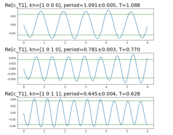
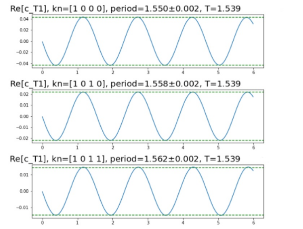
Because of the gauge-fixing, Fourier modes of the vector potential are expected to perfrom simple harmonic motion with known frequencies in the continuum limit. Using the regular HMC kinetic term (with ), the frequencies of the transverse modes are -dependent as follows
| (3.1) |
while using the Fourier accelerated kinetic term eliminates the -dependence of the frequencies such that
| (3.2) |
In Figure 3.1, we examine the numerical evolution of Fourier modes with respect to Monte Carlo time, using the gauge-fixing action of Eq. (2.3). The plots show the simple harmonic motion of the Fourier modes with frequencies described by Eqs. (3.1) and (3.2); and in particular, the dependence of the oscillation frequency on the mode’s spacetime scale vanishes if we use the Fourier accelerated kinetic term.
In order to determine the speedup in the generation of independent gauge configurations, we compare integrated autocorrelation times for the plaquette and the Wilson flowed energy (flow time ) between the GFFA simulations and HMC simulations. We work in a small volume with periodic boundary conditions, at weak coupling . The results, shown in Tables 3.1 and 3.2, indicate a factor of acceleration achieved by GFFA as opposed to HMC.
| steps | trajs | plaq | plaq | E(4) | Accpt | ||
|---|---|---|---|---|---|---|---|
| 10 | 0.6 | 24 | 10030 | 0.783295(37) | 4.51(82) | 20.9(5.4) | 75% |
| 10 | 1.0 | 50 | 10030 | 0.783289(26) | 3.41(30) | 19.0(4.4) | 77.6% |
| 10 | 4.0 | 200 | 8533 | 0.783363(27) | 10.73(61) | 13.0(1.4) | 78% |
| steps | trajs | plaq | plaq | E(4) | M | MC | ||
|---|---|---|---|---|---|---|---|---|
| 10 | 0.6 | 24 | 1911 | 0.783347(45) | 1.26(25) | 3.6(1.0) | 3.0 | 200 |
| 10 | 1.0 | 30 | 5176 | 0.783207(16) | 0.653(31) | 18.6(8.3) | 3.0 | 40 |
| 10 | 0.6 | 24 | 3915 | 0.783404(28) | 1.059(81) | 5.4(1.3) | 5.0 | 200 |
Another observable of interest in the case of periodic boundary conditions is the phase of the average Polyakov loop along a fixed direction, or the Polyakov phase. The Wilson action enjoys a symmetry of the Polyakov phase, whereby the transformation for all the Polyakov loops along the direction leaves the action invariant. While explicitly favors one of the three cube roots of identity, the symmetry should be preserved under our gauge-fixing action if we properly include the compensating Fadev-Poppov term.
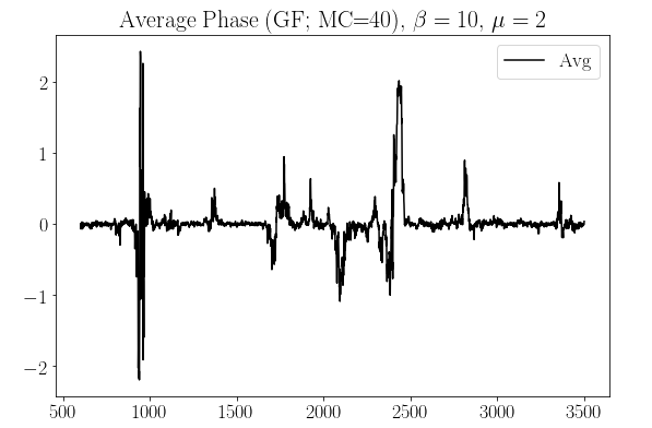
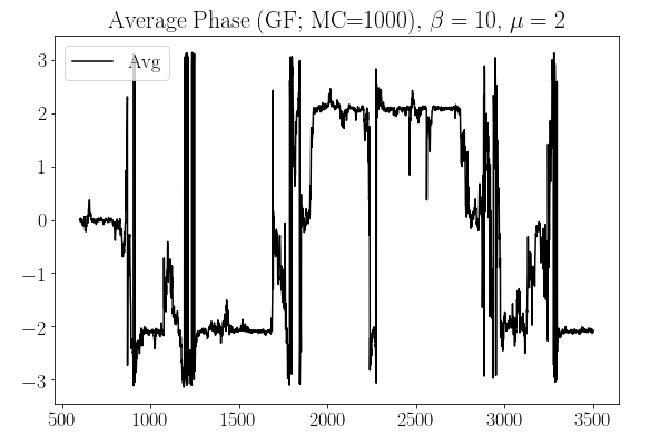
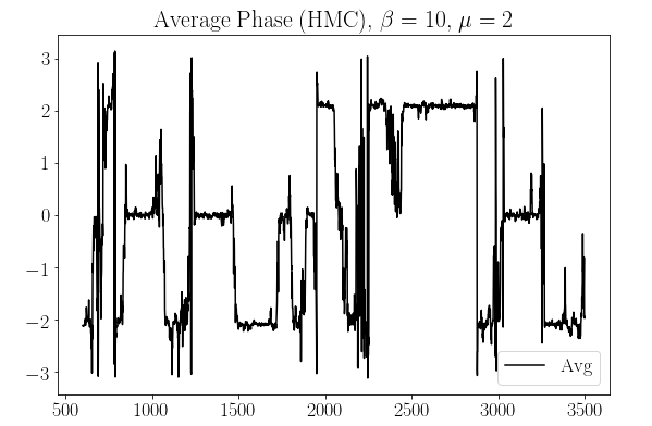
Figure 3.2 examines the evolution of the Polyakov phase in one direction. The HMC simulation shows occasional tunneling between the three cube roots of identity, properly respecting the underlying symmetry of the theory. The gauge-fixed simulations, on the other hand, require a very large number of Monte Carlo samples in estimating the Fadev-Poppov force in order to accurately compensate for the symmetry breaking of and properly tunnel. This presents computational difficulties in our experimental runs, and makes our interpretation of the reduction in autocorrelations seen between Tables 3.1 and 3.2 uncertain. We overcome this obstacle by switching to a lattice with fixed boundary conditions, which is the setup we anticipate eventually working on, as will be explained in the next section. Changing the setup as such has the advantage of completely eliminating the symmetry, and is justified since these Polyakov phases are only nontrivial in high-temperature simulations, but they vanish in the confined regime that our approach aims to accelerate. We can therefore get by using a fewer number of inner Monte Carlo samples, but we must still check for correctness by demanding an accurate estimate of observables as compared to the HMC estimate, and ensuring more accurate convergence when using an increased number of Monte Carlo samples.
4 Fixed Boundary Conditions and Numerical Results
The ultimate goal of our algorithm is to accelerate physically relevant calculations done on large lattices. Fourier acceleration, however, requires all the links in the lattice to be sufficiently close to identity. Even in the weak-coupling limit, a perturbative gauge (such as the Landau gauge of Eq. (2.1)) is still required for the Fourier accelerated kinetic term to match the oscillation modes of the system. If the lattice is large enough to include nonperturbative QCD effects (), finding a perturbative gauge for the entire lattice might be unattainable.
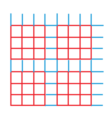
Therefore, in order to accelerate simulations on large lattices, we divide the lattice into many cells which are small enough to be perturbative, as depicted in Figure 4.1. Then, we evolve each of the cells independently, following a checkerboard scheme, using the gauge-fixing action of Eq. (2.3) and the Fourier accelerated kinetic term of Eq. (2.8). If we start with the entire lattice equilibriated with respect to the Wilson action, then, for each cell, we softly fix into Landau gauge by sampling a gauge transformation distributed according to the weight factor , where are the links in the cell (the red links in Figure 4.1). Applying to the sites in the cell fixes the links of the cell to the perturbative Landau gauge and squeezes any nonperturbative effects into its exterior boundary links (the blue links in Figure 4.1). Then, with boundary links held fixed, we evolve the cell according to the gauge-fixing, Fourier accelerated Hamiltonian
| (4.1) |
where includes every plaquette with any of its edges being one of the links in the cell, and is the Fourier accelerated kinetic term in Eq. (2.8), the Fourier modes being those of the cell. To ensure that all the degrees of freedom are updated, we occasionally move around the red cells to include the blue fixed boundary links as part of their evolving links.
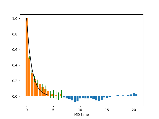
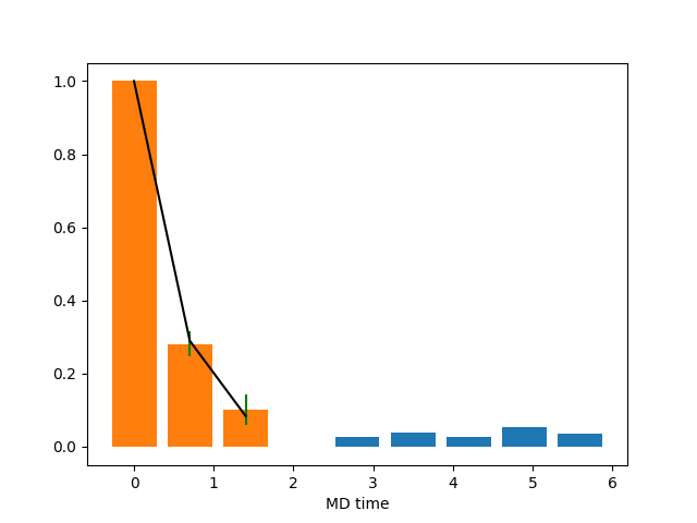
We compare the autocorrelation function and exponential autocorrelation time for the plaquette between HMC runs and GFFA runs in Figure 4.2 and Tables 4.1, 4.2, 4.3, and 4.4. The exponential autocorrelation time is obtained from fitting the autocorrelation function to . In these experiments, we run the simulations on a lattice with fixed boundary conditions that are equilibriated with respect to Wilson action, equivalent to one of the cells in Figure 4.1.
Tables 4.3 and 4.4 indicate a factor of acceleration of the GFFA over the HMC algorithm. Additionally, if we compare the effect of increasing the size of the lattice from to on autocorrelations in the HMC and the GFFA runs, we observe the HMC attaining larger autocorrelations as opposed to the scale-independent GFFA that retains the same efficiency, consistent with a speedup proportional to . This foreshadows an enhanced acceleration factor for the GFFA when working on larger lattices - simulations on which are currently being studied.
| steps | trajs | plaq | plaq | Accpt | ||
|---|---|---|---|---|---|---|
| 10 | 0.5 | 48 | 9431 | 0.783318(56) | 0.810(45) | 97.2% |
| 10 | 1.0 | 96 | 8481 | 0.783313(11) | 1.540(87) | 96.6% |
| steps | trajs | plaq | plaq | M | MC | ||
|---|---|---|---|---|---|---|---|
| 10 | 0.7 | 48 | 2142 | 0.783111(14) | 0.581(47) | 3.0 | 200 |
| steps | trajs | plaq | plaq | Accpt | ||
|---|---|---|---|---|---|---|
| 10 | 0.5 | 48 | 2011 | 0.783395(13) | 0.97(14) | 93.3% |
| 10 | 1.0 | 96 | 1807 | 0.783415(14) | 1.97(30) | 91.5% |
| steps | trajs | plaq | plaq | M | MC | ||
|---|---|---|---|---|---|---|---|
| 10 | 0.7 | 60 | 1296 | 0.783101(10) | 0.569(58) | 3.0 | 200 |
5 Conclusion
In this article, we reviewed the basic formulation of gauge-fixing and Fourier acceleration presented in Ref. [1], and we presented numerical results from simulations on lattices with periodic boundary conditions. The symmetry presents a big computational barrier by requiring a huge number of inner Monte Carlo samples to accurately simulate, so we switch to a lattice with fixed boundary conditions in anticipation of applying GFFA to physically large lattices. Numerical results on lattices with fixed, equilibriated boundary conditions are presented as well, indicating a factor of acceleration in the plaquette observable. Analyzing appropriate observables that probe modes with longer spacetime scales might reveal an enhanced acceleration over the HMC algorithm. It also remains to run simulations on larger lattices that are still perturbative ( at for example), and to check for stronger accelerations corresponding to the increased range of spacetime scales.
References
- [1] Y. Zhao, Numerical Implementation of Gauge-Fixed Fourier Acceleration, PoS LATTICE2018 (2019) 026 [hep-lat/1812.05790].
- [2] D. Zwanziger, Quantization of gauge fields, classical gauge invariance and gluon confinement, Nuclear Physics B 345 (1990) 461.
- [3] C. Parrinello and G. Jona-Lasinio, A modified Faddeev-Popov formula and the Gribov ambiguity, Physics Letters B 251 (1990) 175.
- [4] S. P. Fachin, Quantization of Yang-Mills theory without Gribov copies: Perturbative renormalization, Phys. Rev. D 47 (1993) 3487.