Pole mass renormalon and its ramifications

Abstract

I review the structure of the leading infrared renormalon divergence of the relation between the pole mass and the $\overline{\rm MS}$ mass of a heavy quark, with applications to the top, bottom and charm quark. That the pole quark mass definition must be abandoned in precision computations is a well-known consequence of the rapidly diverging series. The definitions and physics motivations of several leading renormalon-free, short-distance mass definitions suitable for processes involving nearly on-shell heavy quarks are discussed.

1 Introduction

The existence of a short-distance scale $Q\gg\Lambda_{\rm QCD}$ and infrared (IR) finiteness are important requirements for the application of perturbation expansions to strong interaction (QCD) processes, but they are not always enough in practice. The perturbative series is divergent, most likely asymptotic. One of the sources of divergent behaviour, called IR renormalon tHooft:1977xjm ; Parisi:1978az ; David:1983gz ; Mueller:1984vh ; David:1985xj , arises from the sensitivity of the process to the inevitable long-distance scale $\Lambda_{\rm QCD}$. The degree of IR sensitivity limits the ultimate accuracy of the perturbative approximation. For the pole mass of a heavy quark, this observation has been exceptionally important for particle physics phenomenology, leading to a better understanding of quark mass renormalization at scales of order and below the mass of the quark, and to much improved precision in heavy quark and quarkonium physics.

The quark two-point function

$$\int d^{4}x\,e^{ipx}\,\langle\Omega|T(q_{a}(x)\bar{q}_{b}(0))|\Omega\;\rangle\,\stackrel{{\scriptstyle p^{2}\to m^{2}}}{{\rightarrow}}\delta_{ab}\,Z\,\frac{i(\not\!p+m)}{p^{2}-m^{2}}+\mbox{less singular}$$ (1)

has a pole to any order in the perturbative expansion. The location of the pole in the complex $p^{2}$ plane defines the pole mass of the quark, $m$. The pole is shifted off the real axis by a small amount due to the weak decay of the quark, but for the discussion in this article the imaginary part is not relevant and hence will be ignored. The pole mass of a quark is IR-finite Tarrach:1980up ; Kronfeld:1998di . It can be related to other renormalized quark mass definitions order by order in perturbation theory. It is nevertheless not physical, as quarks do not exist as free, asymptotic particle states and the scattering matrix of QCD does not exhibit a pole at $m^{2}$.

It is intuitively obvious that the strong IR physics of QCD, which is not captured by perturbation theory, should contribute an amount $\Lambda_{\rm QCD}$ to hadron masses. For a meson state $M$ composed of $\bar{q}_{i}q_{j}$,

$$M=m_{i}+m_{j}+\mbox{const}\times\Lambda_{\rm QCD}+\ldots,$$ (2)

which renders the notion of the pole mass useless for light quarks with masses $m_{i}\lesssim\Lambda_{\rm QCD}$. However, for mesons containing heavy quarks with $m_{Q}\gg\Lambda_{\rm QCD}$, the pole mass provides a first approximation to the meson mass up to power corrections of relative order $\Lambda_{\rm QCD}/m_{Q}$. Starting from, say, the $\overline{\rm MS}$ mass of the heavy quark, the pole mass represents the perturbatively calculable leading-power approximation to the meson mass, just as the perturbative calculation in terms of quarks and gluons of the total $e^{+}e^{-}\to$ hadrons cross section at high energy does to the physical hadroproduction cross section.

There is a deep connection between power corrections and IR renormalon divergence of the QCD perturbative expansion. The existence of a linear power correction is related to the strong IR renormalon divergence of the pole mass series that was discovered in Beneke:1994sw ; Bigi:1994em and is the subject of this article. In consequence, while the pole mass of a quark appeared as the natural choice for processes involving nearly on-shell heavy quarks, the concept has since largely been abandoned in precision calculations in favour of alternative, (leading) renormalon-free mass definitions.

2 Pole mass series

2.1 Basic definitions

The pole mass $m$ is related to the $\overline{\rm MS}$ mass by

$$m = m(\mu_{m})\bigg{(}1+\sum_{n=1}^{\infty}c_{n}(\mu,\mu_{m},m(\mu_{m}))\,\alpha_{s}^{n}(\mu)\bigg{)}\,.$$ (3)

Here $\alpha_{s}(\mu)$ is the $\overline{\rm MS}$ coupling at scale $\mu$ in QCD with $n_{l}$ light quarks, and $m(\mu_{m})$ stands for the heavy quark $\overline{\rm MS}$ mass evaluated at the scale $\mu_{m}$. In the following I will often set $\mu_{m}=\overline{m}$, where $\overline{m}$ refers to the $\overline{\rm MS}$ mass, evaluated self-consistently at the scale equal to the mass itself, i.e.

$$\overline{m}=m(\overline{m})\,.$$ (4)

We shall see below that the series (3) diverges for any value of $\alpha_{s}\not=0$. Although a proof does not exist for QCD, it is reasonable to assume that it is asymptotic, and approximates the heavy-meson mass up to exponentially small terms in $\alpha_{s}$, equivalent to power corrections in $\Lambda_{\rm QCD}/\overline{m}$. Asymptotic expansions can sometimes be summed using the Borel transform. Given a power series

$$f(\alpha_{s})=\sum_{n=1}^{\infty}c_{n}\alpha_{s}^{n}\,,$$ (5)

the corresponding Borel transform is defined by

$$B[f](t)=\sum_{n=0}^{\infty}c_{n+1}\,\frac{t^{n}}{n!}\,.$$ (6)

By convention, the tree-level term “1” in (3) is excluded from the definition. A factorially divergent series of the form

$$r_{n}=Ka^{n}\Gamma(n+1+b)$$ (7)

has the Borel transform

$$B[f](t)=\frac{K\Gamma(1+b)}{(1-at)^{1+b}}$$ (8)

with a singularity at $t=1/a$. The Borel integral

$$I[f]\equiv\int_{0}^{\infty}dt\,e^{-t/\alpha_{s}}\,B[f](t)$$ (9)

has the same series expansion as $f(\alpha_{s})$ and provides the exact result under suitable conditions. However, for our case of interest, there will be a singularity on the integration contour, rendering the Borel integral as given ill-defined. Deformations of the contour around the pole or branch cut, or the principal-value prescription, result in the ambiguity

$$\delta f\equiv|\mbox{Im}\,I[f]|=\frac{\pi|K|}{a}\,e^{-1/(a\alpha_{s})}\,(a\alpha_{s})^{b}\qquad\mbox{(if $a>0$)}$$ (10)

of the Borel integral, which has the form of a power correction proportional to $\Lambda_{\rm QCD}^{-2\beta_{0}/a}$. The QCD $\beta$-function is defined as $\beta(\alpha_{s})\equiv\mu^{2}\partial\alpha_{s}(\mu)/\partial\mu^{2}=\beta_{0}\alpha_{s}^{2}+\beta_{1}\alpha_{s}^{3}+\ldots$ with $\beta_{0}=-(11-2n_{f}/3)/(4\pi)$. This ambiguity provides a quantitative measure of the limit to the accuracy of a purely perturbative calculation.

The linear power correction to the pole mass therefore corresponds to $a=-2\beta_{0}$. More generally, the pole mass can be regarded as the first term of an asymptotic expansion of the meson mass in powers of $\alpha_{s}$ and $\Lambda_{\rm QCD}/\overline{m}$, which in modern language has a trans-series structure (again, no proof).

2.2 Linear IR sensitivity and the large-$n_{f}$ approximation

To gain intuition, we start from the leading IR renormalon divergence of the one-loop correction to the pole mass with fermion-loop insertions into the gluon line, often referred to as the large-$n_{f}$ approximation. The relevant expression is

$$\Delta m\equiv m-m(\mu) = (-i)g_{s}^{2}C_{F}\mu^{2\epsilon}\int\!\frac{d^{d}k}{(2\pi)^{d}}\,\frac{\gamma^{\mu}(\!\not\!p+\!\not\!k+m)\,\gamma^{\nu}}{k^{2}\,((p-k)^{2}-m^{2})}\big{|}_{p^{2}=m^{2}}\left(g_{\mu\nu}-\frac{k_{\mu}k_{\nu}}{k^{2}}\right)$$ (11)

$$\times\,\sum_{n=0}^{\infty}\left[\beta_{0}\alpha_{s}\ln\left(\frac{-k^{2}e^{-5/3}}{\mu^{2}}\right)\right]^{\!n}+\mbox{counterterms}$$

The all-order $\overline{\rm MS}$ counterterms can be found in Beneke:1994sw . They do not diverge factorially, and can therefore be ignored when discussing the large-$n$ behaviour. Strictly speaking, the fermion-loop insertions provide only the $n_{f}$-dependent part of $\beta_{0}$ in (11). In full QCD, consistency of the trans-series interpretation of short-distance expansions requires the full expression for $\beta_{0}$, as will be seen below. The diagrammatic recovery of the full $\beta_{0}$ is discussed in Beneke:1998ui . The substitution of the full $\beta_{0}$ in fermion bubble-chain diagrams is often referred to as “naive non-abelianization” Broadhurst:1994se ; Beneke:1994qe .

For $p^{2}=m^{2}$ the integral scales as $d^{4}k/k^{3}$ for small $k$. It is thus IR finite, but the contributions from $k$ smaller than $\Lambda_{\rm QCD}$, where perturbation theory is not valid, is of order $\Lambda_{\rm QCD}$. That this should imply that the pole mass cannot be defined to better accuracy than $\mathcal{O}(\Lambda_{\rm QCD})$ was noted in Bigi:1993zi . The connection to the IR renormalon divergence of the perturbative expansion was established shortly after Beneke:1994sw ; Bigi:1994em . Indeed, the increasing power of logarithms in (11) enhance the IR region and yield (after Wick rotation)

$$\int_{0}^{\lambda}dk\,\ln^{n}\!\left(\frac{k^{2}}{\mu^{2}}\right)\stackrel{{\scriptstyle n\gg 1}}{{=}}(-2)^{n}n!\,$$ (12)

with typical $k\sim\mu\,e^{-n}$. One can also take the Borel transform of (11), sum the series, which yields an effective gluon propagator. The exact expression for the Borel transform of $m-m(\mu)$ can be found in Beneke:1994sw . Approximating the integrand to its leading term in the small-$k$ behaviour is sufficient to obtain the dominant IR renormalon singularity at $t=-1/(2\beta_{0})$ (closest to the origin of the Borel plane), resulting in

$$B[\Delta m]=\frac{C_{F}e^{5/6}}{\pi}\,\mu\,\frac{1}{1+2\beta_{0}t}\,.$$ (13)

The corresponding asymptotic behaviour of the series expansion in $\alpha_{s}=\alpha_{s}(\mu)$ is

$$m_{\rm pole}-m_{\overline{\rm MS}}(\mu)=\frac{C_{F}e^{5/6}}{\pi}\,\mu\,\sum_{n}(-2\beta_{0})^{n}\,n!\,\alpha_{s}^{n+1}.$$ (14)

As expected, with $a=-2\beta_{0}>0$ the ambiguity of the Borel integral and hence of the pole mass is proportional to $\Lambda_{\rm QCD}$, independent of the arbitrary renormalization scale $\mu$.

2.3 Exact characterization of the divergence

The relation of IR and ultraviolet (UV) renormalon divergence with the small- and large-momentum behaviour of Feynman diagrams, respectively, allows for a precise characterization of the corresponding singularities in the Borel transform in terms of the factorization properties of observables and correlation functions in these limits. In asymptotically free, renormalizable field theories the UV renormalon singularities occur at $t=n/\beta_{0}<0$ and can be related to local operators of dimension $4+2n$ in the regularized theory expanded for large values of a dimensionful cut-off Parisi:1978bj (see Beneke:1997qd for the case of QCD). If the theory has power UV divergences, as is usually the case for effective field theories, the UV renormalon singularities extend into the positive real axis of the Borel plane. Likewise, the IR behaviour of correlation functions is often amenable to expansions in the ratio of $\Lambda_{\rm QCD}$ and a hard scale, in which case the IR renormalons at $t=-n/\beta_{0}>0$ are related to higher-dimensional terms in the operator product expansion (OPE). For example, for the two-point function of two vector currents,

$$\Pi(Q)=C_{0}(\alpha_{s},Q/\mu)+\frac{1}{Q^{4}}\,C_{GG}(\alpha_{s},Q/\mu)\,\langle\frac{\alpha_{s}}{\pi}G^{2}\rangle(\mu)+O(1/Q^{6}),$$ (15)

the position $t=-2/\beta_{0}$ of the leading IR renormalon divergence of its perturbative series $C_{0}(\alpha_{s},Q/\mu)$ is determined by the dimension (four) of the gluon condensate correction Parisi:1978az ; David:1983gz ; Mueller:1984vh ; David:1985xj . For both, UV and IR renormalons, the parameter $b$ in (8) is determined by the anomalous dimension(s) of the relevant operators. Through renormalization-group equations (RGEs), one can determine the $\alpha_{s}$ dependence of the ambiguity of the Borel integral and thus determine $1/n$ corrections to the leading large-order behaviour in terms of OPE coefficient functions, the anomalous dimensions of all operators of a given dimension, and the beta function coefficients Beneke:1993ee . This leads to the remarkable conclusion that the singular points of the Borel transform due to IR and UV renormalons can be completely specified, except for a set of normalization constants $K$ in (8), whose number matches (at most) the number of operators. They appear as initial conditions of the RGE and should be viewed as non-perturbative Beneke:1993ee ; Grunberg:1992hf .

The application of these ideas to the large-order behaviour of the pole mass series exhibits some unique features: a) due to the linear IR sensitivity, the IR renormalon divergence is particularly strong and dominates over the sign-alternating UV renormalon series; b) the leading IR renormalon singularity at $t=-1/(2\beta_{0})$ involves only a single operator and therefore a single unknown normalization constant; c) the operator has vanishing anomalous dimension, hence the sub-asymptotic $1/n^{k}$ corrections are determined only from the QCD beta-function, which is known to high-order in perturbation theory.

The derivation of these statements in Beneke:1994rs builds on the observation Beneke:1994sw that the leading IR renormalon in the pole mass is related to an UV renormalon pole at the same position $t=-1/(2\beta_{0})$ of the self-energy $\Sigma^{\rm static}$ of the static quark field in heavy quark effective theory (HQET) with Lagrangian

$$\mathcal{L}_{\rm eff}=\bar{h}_{v}iv\cdot Dh_{v}+\mathcal{L}_{\rm light}\,.$$ (16)

This UV renormalon pole exists, because in contrast to full QCD, the static self-energy is linearly UV divergent. The only operator with the required mass dimension three is $\bar{h}_{v}h_{v}$. It follows that the imaginary part of the Borel integral of $\Sigma^{\rm static}$ is given by

$$\mbox{Im}\,I[\Sigma^{\rm static}](\alpha_{s},p,\mu)=E(\alpha_{s},\mu)\,\Sigma^{\rm static}_{\bar{h}h}(\alpha_{s},p,\mu),$$ (17)

where $\Sigma^{\rm static}_{\bar{h}h}$ is the static self-energy with a zero-momentum insertion of $\bar{h}_{v}h_{v}$. The coefficient $E(\alpha_{s},\mu)$ satisfies the RGE

$$\left(\mu^{2}\frac{\partial}{\partial\mu^{2}}+\beta(\alpha_{s})\frac{\partial}{\partial\alpha_{s}}-\gamma_{\bar{h}_{v}h_{v}}(\alpha_{s})\right)E(\alpha_{s},\mu)=0\,.$$ (18)

However, $\gamma_{\bar{h}_{v}h_{v}}$ vanishes to all orders in perturbation theory, since $\bar{h}_{v}h_{v}$ is the conserved heavy quark number current of HQET. This justifies statements b) and c). One then shows that Beneke:1994rs

$$\mbox{Im}\,I[\Delta m]=-E(\alpha_{s},\mu)={\rm const}\times\mu\,\exp\left(\int_{\alpha_{s}}\!dx\frac{1}{2\beta(x)}\right)={\rm const}\times\Lambda_{\rm QCD}.$$ (19)

The $\alpha_{s}$-dependence of the imaginary part of the Borel integral determines the large-order behaviour of the perturbative expansion of $\Delta m$ according to (7), (9) up to a single normalization constant, $N$. Defining

$$c_{n}(\mu,\mu_{m},m(\mu_{m})) \underset{n\to\infty}{\longrightarrow} Nc^{(\rm as)}_{n}(\mu,m(\mu_{m}))\equiv N\frac{\mu}{m(\mu_{m})}\,\tilde{c}^{(\rm as)}_{n}\,,$$ (20)

the result is

$$\tilde{c}_{n+1}^{(\rm as)} = (-2\beta_{0})^{n}\,\frac{\Gamma(n+1+b)}{\Gamma(1+b)}\Bigg{[}1+\frac{s_{1}}{n+b}+\frac{s_{2}}{(n+b)\,(n+b-1)}$$ (21)

$$+\,\frac{s_{3}}{(n+b)\,(n+b-1)\,(n+b-2)}+\ldots\Bigg{]},$$

where Beneke:1994rs ; Beneke:2016cbu $b=-\beta_{1}/(2\beta_{0}^{2})$ and

$$s_{1} = \left(-\frac{1}{2\beta_{0}}\right)\left(-\frac{\beta_{1}^{2}}{2\beta_{0}^{3}}+\frac{\beta_{2}}{2\beta_{0}^{2}}\right),$$ (22)

$$s_{2} = \left(-\frac{1}{2\beta_{0}}\right)^{2}\left(\frac{\beta_{1}^{4}}{8\beta_{0}^{6}}+\frac{\beta_{1}^{3}}{4\beta_{0}^{4}}-\frac{\beta_{1}^{2}\beta_{2}}{4\beta_{0}^{5}}-\frac{\beta_{1}\beta_{2}}{2\beta_{0}^{3}}+\frac{\beta_{2}^{2}}{8\beta_{0}^{4}}+\frac{\beta_{3}}{4\beta_{0}^{2}}\right),$$ (23)

$$s_{3} = \left(-\frac{1}{2\beta_{0}}\right)^{3}\bigg{(}-\frac{\beta_{1}^{6}}{48\beta_{0}^{9}}-\frac{\beta_{1}^{5}}{8\beta_{0}^{7}}-\frac{\beta_{1}^{4}}{6\beta_{0}^{5}}+\frac{\beta_{1}^{4}\beta_{2}}{16\beta_{0}^{8}}+\frac{3\beta_{1}^{3}\beta_{2}}{8\beta_{0}^{6}}+\frac{\beta_{1}^{2}\beta_{2}}{2\beta_{0}^{4}}-\frac{\beta_{1}^{2}\beta_{2}^{2}}{16\beta_{0}^{7}}$$ (24)

$$-\frac{\beta_{1}^{2}\beta_{3}}{8\beta_{0}^{5}}-\frac{\beta_{1}\beta_{2}^{2}}{4\beta_{0}^{5}}-\frac{\beta_{1}\beta_{3}}{3\beta_{0}^{3}}+\frac{\beta_{2}^{3}}{48\beta_{0}^{6}}-\frac{\beta_{2}^{2}}{6\beta_{0}^{3}}+\frac{\beta_{2}\beta_{3}}{8\beta_{0}^{4}}+\frac{\beta_{4}}{6\beta_{0}^{2}}\bigg{)}\,.$$

The pole mass series is particularly simple, because the large-order behaviour is completely determined in terms of the $\beta$-function coefficients. Since the five-loop beta-function coefficient $\beta_{4}$ is now known Baikov:2016tgj ; Herzog:2017ohr ; Luthe:2017ttg , the sub-asymptotic behaviour including $1/n^{3}$ corrections is known. Numerically, for the interesting cases discussed below, the corrections to the leading large-$n$ behaviour do not exceed 3% for $c_{4}$.

2.4 The top, bottom and charm mass series

The normalization constant $N$ in (20) cannot be determined exactly by purely perturbative methods. However, given that the pole-$\overline{\rm MS}$ mass relation (3) is known to the four-loop order Marquard:2015qpa ; Marquard:2016dcn and the asymptotic behaviour is known including $1/n^{3}$ corrections, one may attempt to match the two at $n=4$. In other words, while

$$N = \lim_{n\to\infty}\frac{c_{n}(\mu,\mu_{m},m(\mu_{m}))}{c^{(\rm as)}_{n}(\mu,m(\mu_{m}))}\,,$$ (25)

we evaluate the ratio for $n=4$ and check the stability of the result by comparison with $n=3$ Beneke:2016cbu . In the following, all $n_{l}$ quarks other than the heavy quark will be assumed to be massless. The effect of internal quark mass effects will be discussed below. The coupling $\alpha_{s}$ in (3) is the $\overline{\rm MS}$ coupling in the $n_{l}$-flavour theory. Since the IR theories are different, $N$ is expected to depend on $n_{l}$.

It is interesting to apply this method to the large-$n_{l}$ limit (more precisely, $n_{l}\to-\infty$). In this limit, $b=s_{i}=0$, and $N$ can be calculated exactly from (14) to be

$$\lim_{|n_{l}|\to\infty}N=\frac{C_{F}}{\pi}\times e^{\frac{5}{6}}\,,$$ (26)

which equals $0.97656$ ($C_{F}=4/3$ for $N_{c}=3$). This can be compared to evaluating (25) for $n=4$ at $\mu=\mu_{m}=\overline{m}$, which gives $0.971$ in very good agreement with the exact result. According to (20) the dependence of the asymptotic behaviour on $\mu$ and $\mu_{m}$ is very simple, since the logarithms of $\mu$ in perturbation theory must exponentiate to powers asymptotically. The approximate determination of $N$ is most accurate when choosing $\mu\approx\overline{m}$ and exhibits a plateau around this value Beneke:2016cbu .

With this validation of the method we consider the pole to $\overline{\rm MS}$ mass series for the top, bottom and charm quark, corresponding to $n_{l}=5,4,3$, respectively. For a detailed analysis of the top-quark case, see Beneke:2016cbu . Setting $\mu=\mu_{m}=\overline{m}_{Q}$ for $Q=t,b,c$, one finds

$$N=0.4606\mbox{ (top)},~{}0.5048\mbox{ (bottom)},~{}0.5366\mbox{ (charm)}\,,$$ (27)

where the tiny difference relative to Beneke:2016cbu is due to the inclusion of $s_{3}$, which was not fully available at the time (lack of $\beta_{4}$). A conservative estimate of the uncertainty of these values from the independent variations of $\mu$ and $\mu_{m}$ is $\pm 10\%$ (error symmetrized, see Beneke:2016cbu ), but the accuracy of the large-$n_{l}$ result at $\mu=\mu_{m}=\overline{m}$ suggests that it may be considerably smaller. It is worth noting that $N$ is only half as large as the large-$n_{l}$ result for physical values of $n_{l}$, implying that the intrinsic ambiguity of the pole mass is smaller than inferred from the one-loop correction dressed by fermion loops.

To display the numerical properties of the series, I use the $\overline{\rm MS}$ mass values $\overline{m}_{t}=163.643\,$GeV, $\overline{m}_{b}=4.20\,$GeV and $\overline{m}_{c}=1.28\,$GeV. The strong coupling is taken to be $\alpha_{s}^{(5)}(m_{Z})=0.1180$ at the scale $m_{Z}=91.1876~{}$GeV and evolved with five-loop accuracy to $\overline{m}_{Q}$ including the flavour thresholds at $2\mu_{b}=9.6\,$GeV and $2\mu_{c}=3\,$GeV with the help of RunDec Chetyrkin:2000yt ; Herren:2017osy . The series coefficients are then evaluated at $\mu=\mu_{m}=\overline{m}_{Q}$ in an expansion in $\alpha_{s}^{(5)}(\overline{m}_{t})=0.1084$, $\alpha_{s}^{(4)}(\overline{m}_{b})=0.2246$, $\alpha_{s}^{(3)}(\overline{m}_{c})=0.3889$, for top, bottom and charm, respectively. The result is

$$m_{t} = 163.643+7.531+1.606+0.494+0.194+{\it 0.111+0.079}$$ (28)

$${\it+0.066+{\bf 0.064}+0.070+0.087+0.119+0.178}+\ldots\,{\rm GeV}$$

$$m_{b} = 4.200+0.400+0.199+0.145+{\bf 0.135}+{\it 0.177+0.284}$$ (29)

$${\it+0.539+1.185}+\ldots\,{\rm GeV}$$

$$m_{c} = 1.280+0.211+{\bf 0.202}+0.282+0.510+{\it 1.259+3.798}+\ldots\,{\rm GeV}$$ (30)

for the series expansion of the mass conversion formula. In these expressions the first five numbers correspond to the five exactly known terms including the four-loop order, and the subsequent numbers in italics are obtained from the asymptotic formula (21). By construction, the asymptotic formula agrees with the exact one for the fifth term. The minimal term of the series is highlighted in bold face. The asymptotic formula corresponds to the “prediction”

$$c_{5}=45.43\mbox{ (top, $n_{l}=5$)},~{}73.69\mbox{ (bottom, $n_{l}=4$)},~{}110.56\mbox{ (charm, $n_{l}=3$)}$$ (31)

at $\mu=\mu_{m}=\overline{m}_{Q}$ for the presently unknown five-loop conversion coefficient. The behaviour of the series is illustrated in Figure 1, including an extrapolation of the asymptotic formula to all $n>0$. It is apparent that it is already accurate at the three-loop order, $n=3$.

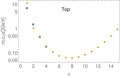
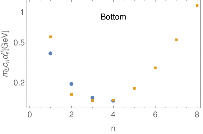
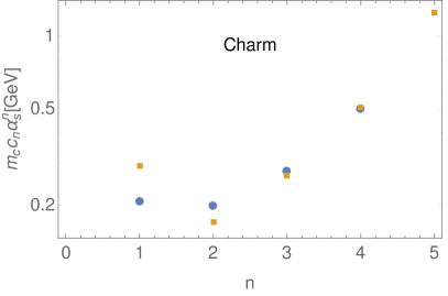
Figure 1: Graphical representation of the series (28) – (30), exhibiting the typical dependence of the size of terms with order of a factorially divergent series. The (blue) circles for $n<5$ represent exactly known terms, the (yellow) squares the asymptotic formula applied to all $n>0$.

Comparing (28) – (30), we observe that the top mass series attains its smallest term at the eighth order in perturbation theory, far beyond the four-loop order currently known. On the other hand, the bottom series reaches its minimal term at this order, while the charm series starts to diverge from the two-loop order, which renders the charm pole mass of limited use for phenomenology. From a pragmatic point of view, the minimal term represents the ultimate accuracy beyond which the purely perturbative use of the pole quark mass ceases to be meaningful. The minimal term scales as $\sqrt{\alpha_{s}(\overline{m}_{Q})}\,\Lambda_{\rm QCD}$ and decreases with larger $m_{Q}$, which reflects the fact that the minimum is shallower in this case. A renormalization-group invariant measure of the intrinsic limitations of the concept of the pole mass can be defined in terms of the ambiguity (10) of the Borel integral of the series,

$$\delta m_{Q}=\frac{\pi N}{|2\beta_{0}|}\times\Lambda_{\rm QCD}^{(n_{f})}\,,$$ (32)

exactly proportional to $\Lambda_{\rm QCD}$, as it should be. Dividing by $\pi$ gives a numerical value close to the minimal term for the top mass series, and this definition of ultimate accuracy has been adopted in Beneke:2016cbu .

Determining the non-perturbative normalization $N$ of the leading pole mass renormalon singularity from matching to the highest known order is perhaps the simplest and most intuitive, but not the only method that has been suggested. I refer to Pineda:2001zq ; Lee:2002sn ; Lee:2003hh ; Hoang:2008yj ; Ayala:2014yxa ; Lee:2015owa ; Hoang:2017suc ; Sumino:2020mxk for other work, noting that earlier work did not have access to four-loop accuracy. As will be seen in Sec. 3.4 below, $N$ is related to a similar leading renormalon constant of the static heavy quark potential by a factor $-1/2$ Beneke:1998rk ; Hoang:1998nz ; PinedaPhD . Some of the quoted works apply this relation to infer $N$ from an analysis of the series expansion of the colour-singlet Coulomb potential. The normalization constants are much more difficult to obtain when there is more than one constant, or an interference of sign-alternating UV and fixed-sign IR renormalon behaviour, as is the case for generic observables. In this case one can resort to simplified parameterizations of the Borel transform as was done for $\tau$-decay spectral moments Beneke:2008ad , but the level of rigour and precision that has been achieved for the pole mass of a heavy quark is unmatched by any other series in QCD.

2.5 Internal quark mass effects

The analysis assumed up to now that the lighter quarks are massless. In low orders of perturbation theory, this is often a good approximation, especially for the top quark pole mass, where $m_{c},m_{b}\ll m_{t}$. (We do not consider the effect of the up, down and strange quark mass and always neglect quark masses smaller than $\Lambda_{\rm QCD}$.) However, in the regime where the series is dominated by the leading renormalon divergence, the typical loop momentum at order $\alpha_{s}^{n+1}$ is of order $m_{Q}e^{-n}$. Internal quark mass effects from the bottom and charm quark are expected to become important in higher orders. The minimal term of the series is attained when the typical loop momentum is of order $\Lambda_{\rm QCD}$. At this scale the theory is a theory of three massless flavours, independent of whether the heavy quark was the top, bottom or charm quark. Hence, the true large-$n$ behaviour of the series beyond the minimal terms is always determined by the $n_{l}=3$ result, and likewise the ambiguity (32) should involve the $\Lambda$-parameter $\Lambda_{\rm QCD}^{(3)}$ in the three-flavour scheme, always excluding the bottom and charm quark, independent of $n_{l}$.

The decoupling of internal quarks with masses $m_{q}$ larger than $\Lambda_{\rm QCD}$ in the renormalon asymptotic behaviour was studied analytically and numerically in the large-$n_{l}$ limit Ball:1995ni , and the described behaviour has been demonstrated. More precisely, the analysis showed that the asymptotic behaviour of the series in a theory with $n_{l}$ quarks of which $n_{m}$ are massive, approaches the series of the theory with $n_{l}-n_{m}$ massless quarks when both are expressed in terms of the $\overline{\rm MS}$ coupling $\alpha_{s}^{(n_{l}-n_{m})}(m_{Q})$ in the $n_{l}-n_{m}$ flavour scheme. However, as noted above the large-$n_{f}$ limit overestimates the normalization of the leading renormalon by about a factor of two. Furthermore, one is rarely interested in the formal large-$n$ behaviour of the series beyond the minimal term, but rather in the approach to it. At such intermediate orders, the typical loop momentum crosses the flavour thresholds, as the order of perturbation theory increases, and the internal quark masses are neither negligible nor decoupled.

The issue is especially relevant for the top quark, since the masses of the bottom and charm quark are too small in relation to $m_{t}$ to express the entire series in terms of the four- or three-flavour coupling. In contrast, one may argue Ayala:2014yxa that the bottom pole to $\overline{\rm MS}$ mass conversion factor should be expressed in terms of $\alpha_{s}^{(3)}(m_{b})$ rather than the four-flavour coupling $\alpha_{s}^{(4)}(m_{b})$. For the two- and three-loop coefficients, for which the mass dependence is known Gray:1990yh ; Bekavac:2007tk ; Fael:2020bgs , this substitution indeed renders the charm mass effect almost negligible. A quantitative investigation of bottom and charm mass effects on the top pole mass series was undertaken in Beneke:2016cbu ; Hoang:2017btd . The following discussion is adapted from Beneke:2016cbu .

I first recall that the numerical series (28) – (30) for $m_{Q}$ include internal loops of $Q$, but are expressed in terms of $\alpha_{s}^{(n_{l})}(\overline{m}_{Q})$, where $n_{l}$ is the number of massless quarks, including bottom and charm for the case of $Q=\,$top ($n_{l}=5$). To estimate the effect of the finite bottom and charm mass, we switch from the five- to the four-flavour scheme at the order, where the typical internal loop momentum is of order $m_{b}$, which is ${\cal O}(\alpha_{s}^{5})$, and from the four- to the three-flavour scheme at ${\cal O}(\alpha_{s}^{6})$. Since the mass effect is not known for $c_{4}$ at the four-loop order, and since $c_{n}$ beyond the four-loop order can only be estimated assuming dominance of the first renormalon (as done above), this implies the following procedure: a) at two and three loops, we include the known mass dependence, but $c_{4}$ is approximated by the massless value. For given top $\overline{\rm MS}$ mass, this increases the top pole mass by 11 (2-loop) + 16 (3-loop) MeV, adopting $\overline{m}_{b}=4.2$ GeV and $\overline{m}_{c}=1.28$ GeV, out of which 8.1 (2-loop) + 11.2 (3-loop) MeV are due to the finite bottom mass, and 2.4 (2-loop) + 4.6 (3-loop) from charm. Since the $c_{n}$ increase as $n_{l}$ decreases, the mass effect is also expected to be positive in higher orders. Hence approximating $c_{4}$ by its massless value underestimates the mass effect. b) At the five-loop order, we use $c_{5}^{(\rm as)}[\alpha_{s}^{(4)}(\overline{m}_{t})]^{5}$ with $c_{5}^{(\rm as)}$ determined by matching to the exactly known four-loop coefficient for $n_{l}=4$, that is with normalization $N_{m}=0.5048$ and beta-function coefficients for the four-flavour theory. c) Beyond five loops, the remainder of the series is computed with the three-flavour scheme coupling $\alpha_{s}^{(3)}(\overline{m}_{t})$ and normalization $N_{m}=0.5366$. Since the bottom and charm quarks are not yet completely decoupled at the five- to seven-loop order, and since an extra quark flavour decreases the $c_{n}$, we expect that b) and c) overestimate the mass effect, since the approximation assumes that bottom and charm are already decoupled completely. The sum of b) and c) adds another 54 MeV to the top pole mass, such that the total mass effect is estimated to be 80 MeV. Explicitly, the series (28) is modified to

$$m_{t} = 163.643+7.531+1.616+0.510+0.194+{\it 0.140+0.106}$$ (33)

$$+\,{\bf 0.094}+{\it 0.096+0.112+0.145+0.209+0.329}+\ldots\,{\rm GeV},$$

where the increasing importance of finite-quark mass effects with order is evident. In case of the top quark pole mass, the decoupling of the bottom and charm quark in internal loops increases the intrinsic uncertainty of the pole mass concept by almost 50% due to the more rapid divergence of the series in the three-massless flavour theory. Note that this ambiguity is independent of the precise value of the bottom and charm mass, as long as $m_{b},m_{c}\gg\Lambda_{\rm QCD}$. This also implies that it is the same for any heavy quark, including the bottom quark, since it depends only on the infrared properties of the theory, which is QCD with three approximately massless flavours.

Since the bottom quark is neither heavy enough to be decoupled in low orders, nor light enough to be ignored, where in both cases a massless approximation can be justified, there is an inherent uncertainty in the above estimate. However, as argued above, the errors in the approximations are expected to go in opposite directions, hence we consider $(80\pm 30)$ MeV a conservative estimate of the total internal bottom and charm quark mass effect on the top pole mass. The 30 MeV error estimate arises from an estimate of the neglected mass effect on $c_{4}$ by extrapolation from the known lower orders. The approximation described here has been checked to work well in models for the series inspired by the large-$n_{l}$ limit.

2.6 Finite width

With the electroweak interaction turned on, the heavy quarks become unstable. In perturbation theory, the pole of the heavy-quark propagator is shifted to

$$m_{*}^{2}=m^{2}-im\Gamma(m)\,,$$ (34)

which defines the pole mass $m$ and on-shell decay width $\Gamma$. Unlike the quark mass, the width is not a parameter of the Standard Model (SM) – for heavy quarks it can be computed in perturbation theory in terms of $m$ and other SM parameters.

The width is negligibly small compared to $m$ except for the top quark, where $\Gamma_{t}\approx 1.4~{}$GeV. The large width $\Gamma_{t}\gg\Lambda_{\rm QCD}$ does not eliminate the renormalon divergence of the top pole mass, as was emphasized in Smith:1996xz . This does not mean that the large width is not relevant, since it does provide a cut-off on IR effects for physical observables. For example, measurements on jets containing top quarks are generically linearly sensitive to $\Lambda_{\rm QCD}$ and accordingly display a strong renormalon divergence, which can be screened by the sizeable width FerrarioRavasio:2018ubr . In effect, as is intuitive, there is simply no quantity, for which the pole mass of a quark is ever the relevant parameter, once the quark’s width is larger than $\Lambda_{\rm QCD}$.

Interestingly, the on-shell width of a quark, $\Gamma(m)$, is itself an observable, which is less sensitive to IR physics than the pole mass. When the final state masses can be neglected, $\Gamma(m)\propto G_{F}^{2}m^{5}$, where $G_{F}$ denotes the Fermi constant. The leading power corrections are of relative order $(\Lambda_{\rm QCD}/m)^{2}$. However, when the series is expressed in terms of the pole mass, an IR renormalon divergence indicating an ambiguity of linear order $\Lambda_{\rm QCD}/m$ appears in the series of QCD corrections to the tree-level width. This ambiguity is spurious and a consequence of using a parameter with stronger IR sensitivity than the observable itself. Once the width of the quark is expressed in terms of the $\overline{\rm MS}$ mass or (better) another leading renormalon-free mass definition such as will be discussed in Sec. 3, the leading renormalon is cancelled Beneke:1994bc , and the series of loop corrections shows a much better behaviour. This is particularly important for the decay width of the bottom and charm quark, for which $\Gamma$ could otherwise be obtained only with large uncertainty.

2.7 Beyond the leading renormalon

Much less is known about the renormalon singularities of the pole mass series beyond $t=-1/(2\beta_{0})$. On general grounds one expects a sign-alternating UV renormalon divergence from a singularity at $t=1/\beta_{0}$, and an IR renormalon singularity at $t=-1/\beta_{0}$ related to the $\Lambda_{\rm QCD}^{2}/m$ kinetic-energy correction to the meson mass (2). The Borel transform of the series is known exactly in the large-$n_{f}$ limit Beneke:1994sw . Table 11 in Beneke:1998ui displays the breakdown of the $n$th order term into the contributions from the first three IR renormalon and the first UV renormalon poles, and the $\overline{\rm MS}$ subtraction terms. At least in the large-$n_{f}$ approximation, the subleading poles never contribute more than one permille of the dominant asymptotics from $t=-1/(2\beta_{0})$ for $n$ beyond the four-loop order. For practical purposes, dealing with the leading singularity appears to be enough.

Curiously, the Borel transform in the large-$n_{f}$ limit does not exhibit the expected next IR renormalon singularity at $t=-1/\beta_{0}$. The authors of Beneke:1994sw speculated that Lorentz invariance might forbid a quadratic power-divergent mixing of the kinetic energy operator $\bar{h}_{v}(iD_{\perp})^{2}h_{v}$ into $\bar{h}_{v}h_{v}$, in which case there would be no matrix element to compensate the ambiguity of the Borel transform from $t=-1/\beta_{0}$, and hence it should be absent. Invoking the virial theorem of HQET, the power-divergent mixing of the kinetic energy operator was related to the one of $\bar{h}_{v}ig_{s}G^{\mu\nu}h_{v}$ into $\bar{h}_{v}h_{v}$ Neubert:1996zy . This work confirms that Lorentz invariance forbids one-loop mixing, which explains the absence of the $t=-1/\beta_{0}$ singularity in the large-$n_{f}$ limit, but also showed that there is no reason for this to hold beyond this limit. Recent investigations Ayala:2019hkn of a remainder series with the leading renormalon subtracted show sign alternation more fitting to UV renormalon behaviour. The question whether the subleading renormalon singularity at $t=-1/\beta_{0}$ is absent or simply suppressed by a loop factor, is therefore still undecided.

3 Renormalon-free “on-shell” masses

Many important properties of heavy quarks are less IR sensitive than the pole quark mass itself – for example, the inclusive decay width discussed above, or the production cross section of a heavy quark-antiquark pair. Their perturbative expansions do not display an IR renormalon singularity at $t=-1/(2\beta_{0})$, leading to rapid divergence, provided they are not expressed in terms of the pole mass. In other words, although the pole mass is IR finite, it is for many purposes not a useful renormalized mass parameter. Instead, one should use a renormalization convention that is not only IR finite but also insensitive to the IR at least at linear order $\Lambda_{\rm QCD}$.

The $\overline{\rm MS}$ definition suggests itself. However, in physical systems where heavy quarks are nearly on-shell and have primarily soft fluctuations, the $\overline{\rm MS}$ mass is not the appropriate choice. Being essentially a bare object, it does not include the short-distance fluctuations, which should have been integrated out to describe soft heavy-quark systems. In practice, this means that the $\overline{\rm MS}$ mass value is too far away (by $\mathcal{O}(\overline{m}_{Q}\alpha_{s})$) from the pole of the heavy-quark propagator. While the spurious pole mass renormalon is eliminated and the asymptotic behaviour improved, there still appear large corrections in low orders. It does not help to evolve the $\overline{\rm MS}$ mass $m(\mu)$ to scales $\mu<\overline{m}$, since the $\overline{\rm MS}$ quark-mass anomalous dimension applies only to the logarithmic evolution above $\overline{m}$.

The resolution to the problem consists in quark mass concepts that are numerically closer to the pole mass, yet are constructed such that their perturbative relation to the $\overline{\rm MS}$ mass is free from the leading IR renormalon. This has several benefits: 1) The concept is unambiguous, at least up to $\mathcal{O}(\alpha_{s}\Lambda_{\rm QCD}^{2}/m)$, which is sufficient for practical purposes. 2) Such masses can be determined accurately from measurements or lattice calculations, and 3) they can be precisely related to the $\overline{\rm MS}$ mass. 4) The impact of light internal quark mass effects is reduced, since the leading IR loop momentum contributions have been removed. The $\overline{\rm MS}$ mass is then the convenient reference parameter (similar to $\alpha_{s}(m_{Z})$ for the strong coupling) to which different leading renormalon-free, “on-shell” mass definitions can be related.

3.1 General considerations

We start from the observation that the asymptotic behaviour (20) of the pole to $\overline{\rm MS}$ mass conversion (3) has a very simple, exact linear dependence on the coupling renormalization scale $\mu$, which follows on very general grounds Beneke:1993ee , as well as on $\mu_{m}$, which appears only through $m(\mu_{m})$. The asymptotic coefficients $\tilde{c}_{n+1}^{(\rm as)}$ themselves in (21) are $m(\mu_{m})$, $\mu$ and $\mu_{m}$ independent. Since the Borel-integral ambiguity of the asymptotic series is always $\Lambda_{\rm QCD}$, we can replace $m(\mu_{m})$ by another scale $\mu_{f}$. We therefore define

$$\delta m_{X}(\mu_{f})=\mu_{f}\sum_{n=1}^{\infty}s_{n}^{X}(\mu/\mu_{f})\,\alpha_{s}^{n}(\mu)=\mu_{f}\sum_{n=1}^{\infty}s_{n}^{X}\,\alpha_{s}^{n}(\mu_{f})\,.$$ (35)

The series coefficients $s_{n}^{X}(\mu/\mu_{f})$ are polynomials of order $n-1$ in $\ln(\mu/\mu_{f})$ and must be chosen to satisfy

$$s^{X}_{n}(\mu/\mu_{f}) \underset{n\to\infty}{\longrightarrow} N\frac{\mu}{\mu_{f}}\,\tilde{c}^{(\rm as)}_{n}\,,$$ (36)

where $N$ and $\tilde{c}^{(\rm as)}_{n}$ are exactly the same as for the coefficients in the pole to $\overline{\rm MS}$ mass relation (20) and (21), respectively. Once such $s_{n}^{X}$ have been found, we can define a leading renormalon-free, “short-distance” mass $m_{X}(\mu_{f})$ by subtracting $\delta m_{X}(\mu_{f})$ from the pole mass $m$:

$$m_{X}(\mu_{f}) \equiv m-\delta m_{X}(\mu_{f})$$ (37)

$$= m(\mu_{m})+\sum_{n=1}^{\infty}\left[m(\mu_{m})\,c_{n}(\mu,\mu_{m},m(\mu_{m}))-\mu_{f}\,s_{n}^{X}(\mu/\mu_{f})\right]\alpha_{s}^{n}(\mu)\,.\qquad$$

By construction the leading IR renormalon divergence of the series cancels in the square bracket. This in turn guarantees that the series that relates $m_{X}(\mu_{f})$ to the $\overline{\rm MS}$ mass $m(\mu_{m})$ is well-behaved (no leading IR renormalon divergence).

The new scale $\mu_{f}$ should be chosen such that $\Lambda_{\rm QCD}\ll\mu_{f}\ll m$. The first inequality is required for perturbativity. The second guarantees that the difference between the pole mass and $m_{X}(\mu_{f})$ is only of order $\mu_{f}\,\alpha_{s}$ and can be made sufficiently small to avoid the problem with the $\overline{\rm MS}$ mass (where $\mu_{f}\sim m$) discussed above. A common feature of all renormalon-free quark mass definitions suitable for the description of nearly on-shell heavy-quark physics is therefore the existence of a new “subtraction scale” $\mu_{f}$ and a linear dependence on this scale. This reflects that the running of the quark mass changes from logarithmic to linear below the scale $m$ in accordance with the fact that the self-energy of a point charge is linearly divergent in the static or non-relativistic regime and turns logarithmic only when the anti-particle fluctuations become relevant in the relativistic theory.

The leading renormalon-free masses satisfy a simple renormalization group equation in the subtraction scale $\mu_{f}$, which may be used to relate $m_{X}(\mu_{f})$ at different scales $\mu_{f2}$, $\mu_{f1}$, when logarithms of $\mu_{f2}/{\mu_{f1}}$ might have to be summed. Defining the anomalous dimension $\gamma_{X}(\alpha_{s})$ through

$$\gamma_{X}(\alpha_{s})=-\frac{dm_{X}(\mu_{f})}{d\mu_{f}}\,,$$ (38)

the general form (35) of the subtraction term yields

$$\gamma_{X}(\alpha_{s}(\mu_{f})) = \sum_{n=1}^{\infty}s_{n}^{X}\,\left[\alpha_{s}^{n}(\mu_{f})+2n\alpha_{s}^{n-1}(\mu_{f})\,\beta(\alpha_{s}(\mu_{f}))\right]$$ (39)

$$= s_{1}^{X}\alpha_{s}(\mu_{f})+[s_{2}^{X}+2s_{1}^{X}\beta_{0}]\,\alpha_{s}^{2}(\mu_{f})+\ldots\,.$$

In the following, I discuss several suitable mass definitions with no claim to completeness. With respect to (2), note that any definition of $\delta m_{X}(\mu_{f})$ automatically yields an unambiguous, renormalon-free definition $\bar{\Lambda}_{X}(\mu_{f})$ of the $\bar{\Lambda}$ parameter that appears in the heavy-quark expansion of the heavy meson mass and many other HQET expressions by the rearrangement

$$M_{Q}=[\underbrace{m_{Q}-\delta m_{X}(\mu_{f})}_{m_{X}(\mu_{f})}]+[\underbrace{\bar{\Lambda}+\delta m_{X}(\mu_{f})}_{\bar{\Lambda}_{X}(\mu_{f})}]+\ldots\,.$$ (40)

This can be turned around: any renormalon-free definition of the HQET parameter $\bar{\Lambda}$ can be turned into a renormalon-free, “short-distance”, on-shell mass definition.

3.2 RS mass

The renormalon subtracted (RS) mass definition Pineda:2001zq is the first of two schemes, which implement the condition (36) in a very direct way. Namely, for RS, one simply defines the $s_{n}^{\rm RS}$ to equal the asymptotic coefficients, that is

$$s_{n}^{\rm RS}(\mu/\mu_{f})=N\frac{\mu}{\mu_{f}}\,\tilde{c}^{(\rm as)}_{n}\,.$$ (41)

While this expression could be used for any $\mu/\mu_{f}$, the implementation proposed in Pineda:2001zq first assumes $\mu=\mu_{f}$, in which case

$$\delta m_{\rm RS}(\mu_{f})=\mu_{f}N\sum_{n=1}^{\infty}\tilde{c}^{(\rm as)}_{n}\,\alpha_{s}^{n}(\mu_{f})\,,$$ (42)

which by construction subtracts the leading renormalon divergence of the series (3), and then replaces $\alpha_{s}(\mu_{f})$ by its series expansion in $\alpha_{s}(\mu)$, where $\mu$ is the scale at which the pole to $\overline{\rm MS}$ series is evaluated. For the bottom and charm mass, the effectiveness of this subtraction is analyzed in detail in Ayala:2014yxa , which also discusses variants of this definition.

A drawback of the RS mass definition is that it needs a precise determination of the normalization $N$, which depends on the method employed and further on the number of light flavours, see (27). To fully define the RS mass, one needs to provide the order to which $\tilde{c}^{(\rm as)}_{n}$ is included according to (21), and specify the value of $N$.

3.3 MSR mass

Another simple realization of the general subtraction condition (36) that avoids the drawback of the RS mass definition is to set the $s_{n}$ equal to $c_{n}$ and simply replace $m(\mu_{r})$ in (20) by the subtraction scale $\mu_{f}$ Hoang:2008yj ; Hoang:2017suc . More precisely, for $\mu=\mu_{f}$, which is assumed here, we define

$$s_{n}^{\rm MSR}{}_{|\mu=\mu_{f}}=c_{n}(\overline{m},\overline{m},\overline{m})\,,$$ (43)

where the pole to $\overline{\rm MS}$ mass conversion coefficients are evaluated at $\mu=\mu_{r}=m(\mu_{r})=\overline{m}$, in which case they are pure numbers. This gives the “practical version” Hoang:2017suc of the MSR mass definition

$$\delta m_{\rm MSR}(\mu_{f})=\mu_{f}\sum_{n=1}^{\infty}c_{n}(\overline{m},\overline{m},\overline{m})\,\alpha_{s}^{n}(\mu_{f})\,.$$ (44)

The requirement (36) is satisfied since according to (20)

$$s_{n}^{\rm MSR}{}_{|\mu=\mu_{f}}=c_{n}(\overline{m},\overline{m},\overline{m}) \underset{n\to\infty}{\longrightarrow} N\,\tilde{c}^{(\rm as)}_{n}\,.$$ (45)

The MSR mass subtraction is straightforward to implement, once the pole to $\overline{\rm MS}$ mass conversion coefficients are given. The MSR mass interpolates between $\overline{m}$ for $\mu_{f}=\overline{m}$ and the pole mass for $\mu_{f}=0$, although the latter limit cannot be taken as the coupling $\alpha_{s}(\mu_{f})$ flows into the strong-coupling regime. The efficiency of the MSR mass subtraction is analyzed in detail in Hoang:2017suc .

Both the RS and MSR mass satisfy a simple renormalization group equation in the subtraction scale, as discussed above. As for $\mu_{f}=\overline{m}$, the MSR mass equals the $\overline{\rm MS}$ mass $\overline{m}$, the relation between $m_{\rm MSR}(\mu_{f})$ and $\overline{m}$ can be obtained conveniently by solving the RGE equation, see Hoang:2017suc . Alternatively, as for the RS scheme, one can replace $\alpha_{s}(\mu_{f})$ in (44) by its series expansion in $\alpha_{s}(\mu)$, where $\mu$ is the scale at which the pole to $\overline{\rm MS}$ series is evaluated, as long as $\ln(\mu/\mu_{f})$ is small enough not to require resummation.

3.4 PS mass

The potential-subtracted (PS) mass Beneke:1998rk is the first of two renormalon-free, short-distance, on-shell masses, which are motivated and defined in terms of another physical quantity than the pole mass. A non-relativistic system of heavy quark and anti-quark in a colour-singlet configuration experiences an attractive potential force, whose leading term is the Coulomb potential. In momentum space,

$$\tilde{V}(\mbox{\boldmath${q}$})=-\frac{4\pi C_{F}}{\mbox{\boldmath${q}$}^{\,2}}\,v_{c}(\alpha_{s}(\mu),q/\mu)\,,$$ (46)

where $q=|\mbox{\boldmath${q}$}|$ and $v_{c}=\alpha_{s}+\ldots$ incorporates the loop corrections to the tree-level potential.

The PS scheme is based on the observation that there is a cancellation of the leading divergent series behaviour in the combination $2m+[V(r)]_{\rm Coulomb}$. This can be seen explicitly at the one-loop order and in the large-$\beta_{0}$ approximation Beneke:1998rk ; Hoang:1998nz ; PinedaPhD , and by a diagrammatic argument at two loops Beneke:1998rk and beyond. The cancellation expresses the fact that while the separation of the total energy of the quarkonium-like system into the quark pole masses and binding energy is ambiguous (as was the case for $m+\bar{\Lambda}$ for a heavy-light system), the total energy is physical and unambiguous. The PS mass at subtraction scale $\mu_{f}$ is defined by

$$m_{\rm PS}(\mu_{f}) = m+\frac{1}{2}\!\int\limits_{|\mbox{\scriptsize$\mbox{\boldmath${q}$}$}\,|<\mu_{f}}\!\!\!\!\frac{d^{3}\mbox{\boldmath${q}$}}{(2\pi)^{3}}\,\tilde{V}(\mbox{\boldmath${q}$})\,,$$ (47)

which removes the leading IR contributions to the self-energy from $q=|\mbox{\boldmath${q}$}|<\mu_{f}$.

The series expansion of $v_{c}(\alpha_{s}(\mu),q/\mu)$ appearing in the Coulomb potential (46) is conventionally written in the form

$$v_{c}(\alpha_{s}(\mu),q/\mu){}_{|\mu=q}=\alpha_{s}(q)+\sum_{n=1}^{\infty}a_{n}\left(\frac{\alpha_{s}(q)}{4\pi}\right)^{\!n+1}+\left(\frac{\alpha_{s}(q)}{4\pi}\right)^{3}8\pi^{2}C_{A}^{3}\ln\frac{\nu^{2}}{\mbox{\boldmath${q}$}^{2}}+\ldots$$ (48)

The coefficients $a_{1,2,3}$ are known, where $a_{3}$ refers to the three-loop colour-singlet Coulomb potential Anzai:2009tm ; Smirnov:2009fh ; Lee:2016cgz . I note that the potential here is not defined in terms of a Wilson loop, but as a matching coefficient Beneke:1998jj to potential non-relativistic QCD (PNRQCD) Pineda:1997bj ; Beneke:1999qg , defined with minimal subtraction. The last term in (48) is the first of an infinite series of terms, which contains an explicit dependence on the factorization or PNRQCD matching scale $\nu$ (to be distinguished from $\mu$), which arises from an IR divergence related to the ultrasoft scale.

Up to the third order to which the potential is currently known, performing the integration over ${q}$ yields Beneke:1998rk ; Beneke:2005hg

$$\delta m_{\rm PS}(\mu_{f}) = -\frac{1}{2}\int_{q\leq\mu_{f}}\frac{d^{3}{\mbox{\boldmath${q}$}}}{(2\pi)^{3}}\,\tilde{V}(\mbox{\boldmath${q}$})$$ (49)

$$= \frac{\mu_{f}C_{F}\alpha_{s}(\mu)}{\pi}\Bigg{[}1+\frac{\alpha_{s}(\mu)}{4\pi}\Big{(}2\beta_{0}\,l_{1}+a_{1}\Big{)}$$

$$+\,\bigg{(}\frac{\alpha_{s}(\mu)}{4\pi}\bigg{)}^{\!2}\bigg{(}4\beta_{0}^{2}\,l_{2}+2\,\Big{(}2a_{1}\beta_{0}+\beta_{1}\Big{)}l_{1}+a_{2}\bigg{)}$$

$$+\,\bigg{(}\frac{\alpha_{s}(\mu)}{4\pi}\bigg{)}^{\!3}\bigg{(}8\beta_{0}^{3}l_{3}+4\Big{(}3a_{1}\beta_{0}^{2}+\frac{5}{2}\beta_{0}\beta_{1}\Big{)}l_{2}+2\Big{(}3a_{2}\beta_{0}+2a_{1}\beta_{1}+\beta_{2}\Big{)}l_{1}$$

$$\hskip 51.21504pt+\,a_{3}+16\pi^{2}C_{A}^{3}\left[\ln\frac{\nu}{\mu_{f}}+1\right]\bigg{)}\Bigg{]},$$

where

$$l_{1} = \ln(\mu/\mu_{f})+1\,,$$

$$l_{2} = \ln^{2}(\mu/\mu_{f})+2\ln(\mu/\mu_{f})+2\,,$$

$$l_{3} = \ln^{3}(\mu/\mu_{f})+3\ln^{2}(\mu/\mu_{f})+6\ln(\mu/\mu_{f})+6\,.$$ (50)

To fully specify the PS mass definition, a value of $\nu$ must be chosen and the standard value is $\nu=\mu_{f}$, which sets the logarithm $\ln(\nu/\mu_{f})$ to zero in the last line. This still leaves a constant term $16\pi^{2}C_{A}^{3}=4263.67...$, which is large compared to $a_{3}=1461.32...$ (quoted for $n_{l}=5$). Since the former is related to an ultrasoft rather than potential effect, another well-motivated choice is $\nu=\mu_{f}e^{-1}$, which nullifies the entire square bracket in the last line, resp. the extra term in (48) at this accuracy. I will refer to this choice as the PS^∗ definition. The difference between the PS and PS^∗ mass is largely irrelevant when the expanded formula (49) is used, since the $n$th order term is dominated by the $l_{i}$ terms, originating from the running coupling in lower order terms, for relevant values of $\mu_{f}$. On the other hand, the difference affects directly the size of the last presently known term in the anomalous dimension and RGE below.

It is instructive to interpret $v_{c}(q)=v_{c}(\alpha_{s}(\mu),q/\mu){}_{|\mu=q}=\alpha_{s}(q)+\ldots$ as an effective coupling, and write the mass subtraction term as

$$\delta m_{\rm PS}(\mu_{f})=\frac{C_{F}}{\pi}\int_{0}^{\mu_{f}}dq\,v_{c}(q)\,.$$ (51)

The $\mu_{f}$ evolution of the PS mass is governed by the anomalous dimension

$$\gamma_{\rm PS}(\alpha_{s}(\mu_{f}))=-\frac{dm_{\rm PS}(\mu_{f})}{d\mu_{f}}=\frac{C_{F}}{\pi}v_{c}(\mu_{f})\,.$$ (52)

The solution is evidently (see (51))

$$\Big{[}\delta m_{\rm PS}(\mu_{f})\Big{]}^{\mu_{f2}}_{\mu_{f1}}=\frac{C_{F}}{\pi}\int^{\mu_{f2}}_{\mu_{f1}}dq\,v_{c}(q)\,,$$ (53)

which allows us to compute $m_{\rm PS}(\mu_{f})$ at widely different scales $\mu_{f1},\mu_{f2}$ without large logarithms by integrating the expansion of $v_{c}(q)$ in terms of the running $\overline{\rm MS}$ coupling $\alpha_{s}(q)$. The leading-logarithmic solution can be expressed in terms of the exponential-integral function.

The PS scheme is especially well-suited for quarkonium-like systems including open $Q\bar{Q}$ systems near threshold, since it subtracts the leading IR contributions explicitly already in low orders of perturbation theory. Prime examples are quarkonium masses at next-to-next-to-next-to-leading order (NNNLO) Beneke:2005hg , the determination of the bottom-quark mass from high moments of the pair production cross section at second Beneke:1999fe and third order Beneke:2014pta in PNRQCD, and in particular precision calculations of top-quark pair production near threshold to NNLO and NNNLO Beneke:1999qg ; Beneke:2015kwa in the PS scheme. For $Q\bar{Q}$ systems near threshold, the scale $\mu_{f}$ should be chosen parametrically of order $mv\sim m\alpha_{s}$ such that $\delta m_{\rm PS}\sim mv^{2}$, in order not to violate the power counting of the non-relativistic expansion. With this choice, the relation (47) is already accurate to order $m\alpha_{s}^{5}$.

3.5 Kinetic mass

The kinetic mass scheme is another physical scheme, in this case related to the physics of semi-leptonic decays of heavy-light mesons Bigi:1994ga ; Bigi:1996si . The pseudoscalar $B$ meson mass has the heavy-quark expansion (cf. (2))

$$m_{B}=m_{b}+\bar{\Lambda}+\frac{\mu_{\pi}^{2}-\mu_{G}^{2}}{2m_{b}}+\ldots,$$ (54)

where $\mu_{\pi}^{2}$ and $\mu_{G}^{2}$ are the $B$-meson matrix elements of the kinetic energy and chromo-magnetic operators, respectively. The kinetic mass can be understood as a perturbative evaluation of this formula, in which the matrix elements include loop momentum integration regions below the scale $\mu_{f}$:

$$m_{\rm kin}(\mu_{f}) = m\underbrace{-[\bar{\Lambda}(\mu_{f})]_{\rm pert}-\left[\frac{\mu_{\pi}^{2}(\mu_{f})}{2m_{\rm kin}(\mu_{f})}\right]_{\rm pert}}_{-\delta m_{\rm kin}(\mu_{f})}+\ldots.$$ (55)

The matrix elements on the right-hand side subtract the long-distance sensitive contributions to the pole mass order by order in $\mu_{f}/m_{Q}$ and $\alpha_{s}$. Comparing to (40), we note that the kinetic mass definition not only subtracts the leading IR renormalon divergence through $[\bar{\Lambda}(\mu_{f})]_{\rm pert}$, but also the IR sensitivity at subleading power $\Lambda_{\rm QCD}^{2}/m$.

Up to now the discussion has been general. The kinetic scheme is defined by providing a concrete prescription for calculating the perturbative matrix elements in terms of the perturbative evaluation of short-distance observables. It relies on the fact that the $\bar{\Lambda}$ parameter and kinetic-energy matrix element appear in the heavy-quark expansion of the dilepton-differential spectrum of inclusive semi-leptonic $B\to X_{c}\ell\bar{\nu}$ decays Manohar:1993qn ; Blok:1993va , which can be constructed from the imaginary part of the two-point function of the $b\to c$ transition current. The convention for the kinetic mass used in the literature employs an indirect definition of the matrix elements through heavy flavour sum rules Bigi:1994ga ; Bigi:1996si in the small-velocity limit, which is rather complicated when compared with the other three mass definitions above. The central quantity is the forward amplitude

$$T(q) = \frac{i}{2m_{Q}}\int{\rm d}^{4}{x\,}e^{-iqx}\langle Q|TJ(x)J^{\dagger}(0)|Q\rangle$$ (56)

and its discontinuity

$$W(q) = 2\,\mbox{Im}\,[T(q)]\,.$$ (57)

Since the perturbative matrix elements (55) to be computed are spin-independent and universal, instead of the physical V-A current, one can define the kinetic scheme by adopting the scalar current $J=QQ^{\prime}$ provided $Q$ and $Q^{\prime}$ are heavy. To simplify further, one can set $Q^{\prime}=Q$ and compute the forward scattering of the heavy quark off the current $J$ with momentum $q=(q^{0},\mbox{\boldmath${q}$})$ in the limit when $\mbox{\boldmath${v}$}=\mbox{\boldmath${q}$}/m_{Q}\ll 1$. To isolate the IR region of the final state momenta, the total energy of the quark and gluon final state $X$ excluding the heavy quark $Q$ is restricted to

$$\omega\equiv q^{0}-\Big{[}\sqrt{m_{Q}^{2}+\mbox{\boldmath${q}$}^{2}}-m_{Q}\Big{]}<\mu_{f}\,.$$ (58)

Employing the variables $(\omega,\mbox{\boldmath${v}$})$ instead of $(q^{0},\mbox{\boldmath${q}$})$, the mass subtractions are defined in terms of the double limit of the first moments of the spectral function:

$$[\bar{\Lambda}(\mu_{f})]_{\rm pert} = \lim_{\mbox{\boldmath${v}$}\to 0}\lim_{m_{Q}\to\infty}\frac{2}{\mbox{\boldmath${v}$}\,^{2}}\frac{\displaystyle\int_{0}^{\mu_{f}}d\omega\,\omega\,W(\omega,\mbox{\boldmath${v}$})}{\displaystyle\int_{0}^{\mu_{f}}d\omega\,W(\omega,\mbox{\boldmath${v}$})}\,,$$ (59)

$$[\mu_{\pi}^{2}(\mu)]_{\rm pert} = \lim_{\mbox{\boldmath${v}$}\to 0}\lim_{m_{b}\to\infty}\frac{3}{\mbox{\boldmath${v}$}\,^{2}}\frac{\displaystyle\int_{0}^{\mu_{f}}d\omega\,\omega^{2}\,W(\omega,\mbox{\boldmath${v}$})}{\displaystyle\int_{0}^{\mu_{f}}d\omega\,W(\omega,\mbox{\boldmath${v}$})}\,.$$ (60)

The demonstration that the right-hand sides of these equations can be identified with the subtracted $\bar{\Lambda}$ and kinetic-energy parameters, which appear in the heavy-quark expansion of the meson mass, is given in Bigi:1996si . It is sufficient to compute $W(\omega,\mbox{\boldmath${v}$})$ in an expansion in $\omega,|\mbox{\boldmath${q}$}|\ll m_{Q}$ to order

$$W(\omega,\mbox{\boldmath${v}$})=W_{\rm virt}(\mbox{\boldmath${v}$})\delta(\omega)+\frac{\mbox{\boldmath${v}$}^{2}}{\omega}W_{\rm real}\Theta(\omega)+\mathcal{O}(\omega^{0},\mbox{\boldmath${v}$}^{4})\,.$$ (61)

The two-loop computation Czarnecki:1997sz has been known for some time, but the three-loop result has been obtained only recently Fael:2020iea ; Fael:2020njb . Different from the other three mass schemes, the $\mathcal{O}(\alpha_{s}^{4})$ term of $\delta m_{\rm kin}(\mu_{f})$ is presently not available.

The kinetic scheme is especially well-suited for observables derived from semi-leptonic decays of heavy quarks, since it subtracts the leading IR contributions explicitly already in low orders of perturbation theory. Initially, it was suggested to eliminate the leading renormalon divergence from the semi-leptonic width by replacing the pole mass by the $\overline{\rm MS}$ mass Ball:1995wa , but this does not improve the behaviour in low orders. The comparison to the series convergence when renormalon-free on-shell masses are used (Table 2 of Beneke:1999zr ) clearly shows the latter’s advantage. The kinetic scheme was used for bottom quark mass and $|V_{cb}|$ determinations at second order Gambino:2013rza . Recently, the semi-leptonic decay width was calculated to NNNLO and the effectiveness of the kinetic mass scheme was demonstrated for the inclusive rate for the first time at this order Fael:2020tow .

3.6 Comparison

Table 1: Comparison of top quark mass definitions for $\mu_{f}=20\,$GeV for given $\overline{\rm MS}$ mass $\overline{m}_{t}$. $\alpha_{s}(m_{Z})=(0.1180\pm 0.0010)$. “$n$-loop” refers to the value of the $n$-loop contribution to the mass. All numbers in GeV.

top	$\overline{m}_{t}$	1-loop	2-loop	3-loop	4-loop	Sum
$m_{t}$	163.643	7.531	1.606	0.494	0.194	$173.468^{+0.101}_{-0.101}$
$m_{t,\rm RS}$	163.643	6.123	1.079	0.239	0.048	$171.132^{+0.071}_{-0.071}$
$m_{t,\rm MSR}$	163.643	6.611	1.154	0.242	0.042	$171.691^{+0.076}_{-0.076}$
$m_{t,\rm PS}$	163.643	6.611	1.190	0.265	0.048	$171.756^{+0.077}_{-0.077}$
$m_{t,\rm PS^{*}}$	163.643	6.611	1.190	0.265	0.051	$171.759^{+0.078}_{-0.077}$
$m_{t,\rm kin}$	163.643	6.248	0.995	0.180	—	$171.065^{+0.068}_{-0.068}$

Table 2: Comparison of bottom quark mass definitions for $\mu_{f}=2\,$GeV for given $\overline{\rm MS}$ mass $\overline{m}_{b}$. $\alpha_{s}(m_{Z})=(0.1180\pm 0.0010)$. “$n$-loop” refers to the value of the $n$-loop contribution to the mass. All numbers in GeV.

bottom	$\overline{m}_{b}$	1-loop	2-loop	3-loop	4-loop	Sum
$m_{b}$	4.200	0.400	0.199	0.145	0.135	$5.079^{+0.031}_{-0.029}$
$m_{b,\rm RS}$	4.200	0.126	0.065	0.028	0.007	$4.425^{+0.006}_{-0.006}$
$m_{b,\rm MSR}$	4.200	0.210	0.062	0.020	0.001	$4.493^{+0.007}_{-0.007}$
$m_{b,\rm PS}$	4.200	0.210	0.080	0.032	0.000	$4.521^{+0.008}_{-0.008}$
$m_{b,\rm PS^{*}}$	4.200	0.210	0.080	0.032	0.005	$4.526^{+0.008}_{-0.008}$
$m_{b,\rm kin}$	4.200	0.101	0.004	-0.002	—	$4.303^{+0.002}_{-0.002}$

Table 3: Comparison of charm quark mass definitions for $\mu_{f}=1\,$GeV for given $\overline{\rm MS}$ mass $\overline{m}_{c}$. $\alpha_{s}(m_{Z})=(0.1180\pm 0.0010)$. “$n$-loop” refers to the value of the $n$-loop contribution to the mass. All numbers in GeV.

charm	$\overline{m}_{c}$	1-loop	2-loop	3-loop	4-loop	Sum
$m_{c}$	1.280	0.211	0.202	0.282	0.510	$2.486^{+0.126}_{-0.109}$
$m_{c,\rm RS}$	1.280	-0.017	0.037	0.026	0.005	$1.331^{+0.006}_{-0.005}$
$m_{c,\rm MSR}$	1.280	0.046	0.022	0.010	-0.002	$1.356^{+0.004}_{-0.004}$
$m_{c,\rm PS}$	1.280	0.046	0.052	0.034	-0.019	$1.393^{+0.006}_{-0.006}$
$m_{c,\rm PS^{*}}$	1.280	0.046	0.052	0.034	0.002	$1.414^{+0.009}_{-0.008}$
$m_{c,\rm kin}$	1.280	-0.073	-0.062	-0.017	—	$1.128^{+0.008}_{-0.009}$

Once any of the leading renormalon-free, on-shell, short-distance masses has been determined from some observable, one is eventually interested in converting them to the $\overline{\rm MS}$ reference mass $\overline{m}$. Over the past twenty years the accuracy of the mass definitions and observables has improved by one order (typically from two-loop to three-loop, and three-loop to four-loop for the pole to $\overline{\rm MS}$ mass series). It is therefore timely to update and extend the comparison Beneke:1999zr of different definitions (see also Marquard:2016dcn ).

The purpose of the following comparison is to display the good behaviour of the relation between the various subtracted masses and the $\overline{\rm MS}$ mass contrary to the pole mass series (28) – (30). As above, the $\overline{\rm MS}$ masses are fixed to $\overline{m}_{t}=163.643\,$GeV, $\overline{m}_{b}=4.20\,$GeV and $\overline{m}_{c}=1.28\,$GeV. The strong coupling is taken to be $\alpha_{s}^{(5)}(m_{Z})=0.1180\pm 0.0010$ at the scale $m_{Z}=91.1876~{}$GeV, and the series coefficients are evaluated at $\mu=\mu_{m}=\overline{m}$ in an expansion in $\alpha_{s}^{(5)}(\overline{m}_{t})=0.1084$, $\alpha_{s}^{(4)}(\overline{m}_{b})=0.2246$, $\alpha_{s}^{(3)}(\overline{m}_{c})=0.3889$, for top, bottom and charm, respectively. The subtraction scale $\mu_{f}$ is chosen to be $\mu_{f}=(20,2,1)\,$GeV for top, bottom and charm, equal for all mass definitions for the sake of comparison, even if different “canonical” values are often adopted for the different schemes. Internal mass effects are neglected, since they are not always known with comparable precision. In case of mass schemes originally defined in terms of $\alpha_{s}(\mu_{f})$, the series have been converted into expansions in $\alpha_{s}(\overline{m}_{Q})$ with the required four-loop accuracy.

I use private code for the RS, MSR and PS mass. The RS and PS scheme (for $\nu=\mu_{f}$) is also implemented in CRunDec3.1 Herren:2017osy and the PS mass also in $\tt{QQbar\_threshold}$ Beneke:2016kkb . In case of the RS scheme I adapted the normalization constants $N_{m}=0.563$ ($n_{l}=3$), $N_{m}=0.547$ ($n_{l}=4$), $N_{m}=0.527$ ($n_{l}=3$) given in Ayala:2014yxa (and hard-coded in CRunDec3.1) to the values from (27). Finally, the kinetic mass $m_{\rm kin}$ is implemented for massless internal quarks with CRunDec3.1’s mMS2mKIN[$\overline{m}_{Q}$, 0, 0, "[as]"*$\alpha_{s}^{(n_{l})}(\overline{m}_{Q})$, $\overline{m}_{Q}$, $\mu_{f}$, $n_{l}$, $n_{l}$, 3, ""] call, presently available only to three-loop accuracy.

The results are summarized in Tables 3 to 3. It is evident that in terms of the size of mass corrections up to the shown four-loop order, all mass schemes are rather similar with exception of the kinetic scheme. In all cases, one observes a spectacular improvement of convergence relative to the pole mass series given in the first line. One expects the cancellation of the leading renormalon to become more and more effective in higher orders measured relative to the order of the minimal term, which can be seen explicitly by comparing the top, bottom and charm tables. The effect is particularly dramatic for the charm mass, for which the pole mass series starts diverging beyond the two-loop order, while the renormalon-subtracted masses are still well-behaved at the fourth order, with corrections in the few MeV range. The top pole mass series is still in the regime of decreasing coefficients at the four-loop order, albeit slowly, hence the relative improvement of the subtraction should increase in the next orders. The four-loop coefficient is typically $(40-50)\,$MeV, but the size of the next unknown term can be assumed to be small enough relative to the experimental precision that can be attained in the future, even from the scan of the pair production cross section in $e^{+}e^{-}$ collisions Simon:2019axh .

“Sum” in the last column of the tables refers to the sum of the terms up to the four-loop order shown, and the error attached quantifies the variation of the sum under a variation of $\alpha_{s}(m_{Z})$ by $\pm 0.001$. It is apparent that once leading renormalon-free, on-shell masses are employed, the limitation of the accuracy of their relations to the $\overline{\rm MS}$ mass is (currently) no longer determined by the convergence of the expansion, but by the precision of $\alpha_{s}(m_{Z})$. For the case of the top quark, this uncertainty is mainly caused by the large one-loop correction of a few GeV to be compared to the ultimate precision to which the subtracted masses can be obtained theoretically and (in principle) experimentally. Unlike the bottom and charm masses, to make use of this precision requires better knowledge of the strong coupling.

Acknowledgement.

I thank F. Herren and M. Steinhauser for helpful communication on RunDec’s implementation of the kinetic scheme.

References

- (1) G. ’t Hooft, Can We Make Sense Out of Quantum Chromodynamics?, in: The Whys of subnuclear physics. Springer, Subnuclear Series 15 (1979) 943.
- (2) G. Parisi, On Infrared Divergences, Nucl. Phys. B 150 (1979) 163–172.
- (3) F. David, On the Ambiguity of Composite Operators, IR Renormalons and the Status of the Operator Product Expansion, Nucl. Phys. B 234 (1984) 237–251.
- (4) A. H. Mueller, On the Structure of Infrared Renormalons in Physical Processes at High-Energies, Nucl. Phys. B 250 (1985) 327–350.
- (5) F. David, The Operator Product Expansion and Renormalons: A Comment, Nucl. Phys. B 263 (1986) 637–648.
- (6) R. Tarrach, The Pole Mass in Perturbative QCD, Nucl. Phys. B 183 (1981) 384–396.
- (7) A. S. Kronfeld, The Perturbative pole mass in QCD, Phys. Rev. D 58 (1998) 051501, [hep-ph/9805215].
- (8) M. Beneke and V. M. Braun, Heavy quark effective theory beyond perturbation theory: Renormalons, the pole mass and the residual mass term, Nucl. Phys. B426 (1994) 301–343, [hep-ph/9402364].
- (9) I. I. Y. Bigi, M. A. Shifman, N. G. Uraltsev and A. I. Vainshtein, The Pole mass of the heavy quark. Perturbation theory and beyond, Phys. Rev. D50 (1994) 2234–2246, [hep-ph/9402360].
- (10) M. Beneke, Renormalons, Phys. Rept. 317 (1999) 1–142, [hep-ph/9807443].
- (11) M. Beneke and V. M. Braun, Renormalons and power corrections, hep-ph/0010208.
- (12) D. J. Broadhurst and A. G. Grozin, Matching QCD and HQET heavy - light currents at two loops and beyond, Phys. Rev. D 52 (1995) 4082–4098, [hep-ph/9410240].
- (13) M. Beneke and V. M. Braun, Naive non-abelianization and resummation of fermion bubble chains, Phys. Lett. B348 (1995) 513–520, [hep-ph/9411229].
- (14) I. I. Y. Bigi and N. G. Uraltsev, Anathematizing the Guralnik-Manohar bound for anti-Lambda, Phys. Lett. B 321 (1994) 412–416, [hep-ph/9311337].
- (15) G. Parisi, Singularities of the Borel Transform in Renormalizable Theories, Phys. Lett. B 76 (1978) 65–66.
- (16) M. Beneke, V. M. Braun and N. Kivel, Large order behavior due to ultraviolet renormalons in QCD, Phys. Lett. B 404 (1997) 315–320, [hep-ph/9703389].
- (17) M. Beneke, Renormalization scheme invariant large order perturbation theory and infrared renormalons in QCD, Phys. Lett. B 307 (1993) 154–160.
- (18) G. Grunberg, The Renormalization scheme invariant Borel transform and the QED renormalons, Phys. Lett. B 304 (1993) 183–188.
- (19) M. Beneke, More on ambiguities in the pole mass, Phys. Lett. B344 (1995) 341–347, [hep-ph/9408380].
- (20) M. Beneke, P. Marquard, P. Nason and M. Steinhauser, On the ultimate uncertainty of the top quark pole mass, Phys. Lett. B 775 (2017) 63–70, [1605.03609].
- (21) P. A. Baikov, K. G. Chetyrkin and J. H. Kühn, Five-Loop Running of the QCD coupling constant, Phys. Rev. Lett. 118 (2017) 082002, [1606.08659].
- (22) F. Herzog, B. Ruijl, T. Ueda, J. A. M. Vermaseren and A. Vogt, The five-loop beta function of Yang-Mills theory with fermions, JHEP 02 (2017) 090, [1701.01404].
- (23) T. Luthe, A. Maier, P. Marquard and Y. Schröder, The five-loop Beta function for a general gauge group and anomalous dimensions beyond Feynman gauge, JHEP 10 (2017) 166, [1709.07718].
- (24) P. Marquard, A. V. Smirnov, V. A. Smirnov and M. Steinhauser, Quark Mass Relations to Four-Loop Order in Perturbative QCD, Phys. Rev. Lett. 114 (2015) 142002, [1502.01030].
- (25) P. Marquard, A. V. Smirnov, V. A. Smirnov, M. Steinhauser and D. Wellmann, -on-shell quark mass relation up to four loops in QCD and a general SU gauge group, Phys. Rev. D 94 (2016) 074025, [1606.06754].
- (26) K. G. Chetyrkin, J. H. Kühn and M. Steinhauser, RunDec: A Mathematica package for running and decoupling of the strong coupling and quark masses, Comput. Phys. Commun. 133 (2000) 43–65, [hep-ph/0004189].
- (27) F. Herren and M. Steinhauser, Version 3 of RunDec and CRunDec, Comput. Phys. Commun. 224 (2018) 333–345, [1703.03751].
- (28) A. Pineda, Determination of the bottom quark mass from the Upsilon(1S) system, JHEP 06 (2001) 022, [hep-ph/0105008].
- (29) T. Lee, Surviving the renormalon in heavy quark potential, Phys. Rev. D 67 (2003) 014020, [hep-ph/0210032].
- (30) T. Lee, Heavy quark mass determination from the quarkonium ground state energy: A Pole mass approach, JHEP 10 (2003) 044, [hep-ph/0304185].
- (31) A. H. Hoang, A. Jain, I. Scimemi and I. W. Stewart, Infrared Renormalization Group Flow for Heavy Quark Masses, Phys. Rev. Lett. 101 (2008) 151602, [0803.4214].
- (32) C. Ayala, G. Cvetic and A. Pineda, The bottom quark mass from the system at NNNLO, JHEP 09 (2014) 045, [1407.2128].
- (33) T. Lee, Flavor dependence of normalization constant for an infrared renormalon, Phys. Lett. B742 (2015) 327–329, [1502.02698].
- (34) A. H. Hoang, A. Jain, C. Lepenik, V. Mateu, M. Preisser, I. Scimemi et al., The MSR mass and the renormalon sum rule, JHEP 04 (2018) 003, [1704.01580].
- (35) Y. Sumino and H. Takaura, On renormalons of static QCD potential at and , JHEP 05 (2020) 116, [2001.00770].
- (36) M. Beneke, A Quark mass definition adequate for threshold problems, Phys. Lett. B 434 (1998) 115–125, [hep-ph/9804241].
- (37) A. H. Hoang, M. C. Smith, T. Stelzer and S. Willenbrock, Quarkonia and the pole mass, Phys. Rev. D 59 (1999) 114014, [hep-ph/9804227].
- (38) A. Pineda, PhD Thesis, University of Barcelona (1998) .
- (39) M. Beneke and M. Jamin, alpha(s) and the tau hadronic width: fixed-order, contour-improved and higher-order perturbation theory, JHEP 09 (2008) 044, [0806.3156].
- (40) P. Ball, M. Beneke and V. M. Braun, Resummation of corrections in QCD: Techniques and applications to the tau hadronic width and the heavy quark pole mass, Nucl. Phys. B452 (1995) 563–625, [hep-ph/9502300].
- (41) N. Gray, D. J. Broadhurst, W. Grafe and K. Schilcher, Three Loop Relation of Quark (Modified) Ms and Pole Masses, Z. Phys. C 48 (1990) 673–680.
- (42) S. Bekavac, A. Grozin, D. Seidel and M. Steinhauser, Light quark mass effects in the on-shell renormalization constants, JHEP 10 (2007) 006, [0708.1729].
- (43) M. Fael, K. Schönwald and M. Steinhauser, Exact results for and with two mass scales and up to three loops, JHEP 10 (2020) 087, [2008.01102].
- (44) A. H. Hoang, C. Lepenik and M. Preisser, On the Light Massive Flavor Dependence of the Large Order Asymptotic Behavior and the Ambiguity of the Pole Mass, JHEP 09 (2017) 099, [1706.08526].
- (45) M. C. Smith and S. S. Willenbrock, Top quark pole mass, Phys. Rev. Lett. 79 (1997) 3825–3828, [hep-ph/9612329].
- (46) S. Ferrario Ravasio, P. Nason and C. Oleari, All-orders behaviour and renormalons in top-mass observables, JHEP 01 (2019) 203, [1810.10931].
- (47) M. Beneke, V. M. Braun and V. I. Zakharov, Bloch-Nordsieck cancellations beyond logarithms in heavy particle decays, Phys. Rev. Lett. 73 (1994) 3058–3061, [hep-ph/9405304].
- (48) M. Neubert, Exploring the invisible renormalon: Renormalization of the heavy quark kinetic energy, Phys. Lett. B 393 (1997) 110–118, [hep-ph/9610471].
- (49) C. Ayala, X. Lobregat and A. Pineda, Hyperasymptotic approximation to the top, bottom and charm pole mass, Phys. Rev. D 101 (2020) 034002, [1909.01370].
- (50) C. Anzai, Y. Kiyo and Y. Sumino, Static QCD potential at three-loop order, Phys. Rev. Lett. 104 (2010) 112003, [0911.4335].
- (51) A. V. Smirnov, V. A. Smirnov and M. Steinhauser, Three-loop static potential, Phys. Rev. Lett. 104 (2010) 112002, [0911.4742].
- (52) R. N. Lee, A. V. Smirnov, V. A. Smirnov and M. Steinhauser, Analytic three-loop static potential, Phys. Rev. D 94 (2016) 054029, [1608.02603].
- (53) M. Beneke, New results on heavy quarks near threshold, in 3rd Workshop on Continuous Advances in QCD (QCD 98), 6, 1998. hep-ph/9806429.
- (54) A. Pineda and J. Soto, Effective field theory for ultrasoft momenta in NRQCD and NRQED, Nucl. Phys. B Proc. Suppl. 64 (1998) 428–432, [hep-ph/9707481].
- (55) M. Beneke, A. Signer and V. A. Smirnov, Top quark production near threshold and the top quark mass, Phys. Lett. B 454 (1999) 137–146, [hep-ph/9903260].
- (56) M. Beneke, Y. Kiyo and K. Schuller, Third-order Coulomb corrections to the S-wave Green function, energy levels and wave functions at the origin, Nucl. Phys. B 714 (2005) 67–90, [hep-ph/0501289].
- (57) M. Beneke and A. Signer, The Bottom MS-bar quark mass from sum rules at next-to-next-to-leading order, Phys. Lett. B 471 (1999) 233–243, [hep-ph/9906475].
- (58) M. Beneke, A. Maier, J. Piclum and T. Rauh, The bottom-quark mass from non-relativistic sum rules at NNNLO, Nucl. Phys. B 891 (2015) 42–72, [1411.3132].
- (59) M. Beneke, Y. Kiyo, P. Marquard, A. Penin, J. Piclum and M. Steinhauser, Next-to-Next-to-Next-to-Leading Order QCD Prediction for the Top Antitop -Wave Pair Production Cross Section Near Threshold in Annihilation, Phys. Rev. Lett. 115 (2015) 192001, [1506.06864].
- (60) I. I. Y. Bigi, M. A. Shifman, N. G. Uraltsev and A. I. Vainshtein, Sum rules for heavy flavor transitions in the SV limit, Phys. Rev. D 52 (1995) 196–235, [hep-ph/9405410].
- (61) I. I. Y. Bigi, M. A. Shifman, N. Uraltsev and A. I. Vainshtein, High power of in beauty widths and limit, Phys. Rev. D 56 (1997) 4017–4030, [hep-ph/9704245].
- (62) A. V. Manohar and M. B. Wise, Inclusive semileptonic B and polarized Lambda(b) decays from QCD, Phys. Rev. D 49 (1994) 1310–1329, [hep-ph/9308246].
- (63) B. Blok, L. Koyrakh, M. A. Shifman and A. I. Vainshtein, Differential distributions in semileptonic decays of the heavy flavors in QCD, Phys. Rev. D 49 (1994) 3356, [hep-ph/9307247].
- (64) A. Czarnecki, K. Melnikov and N. Uraltsev, Non-abelian dipole radiation and the heavy quark expansion, Phys. Rev. Lett. 80 (1998) 3189–3192, [hep-ph/9708372].
- (65) M. Fael, K. Schönwald and M. Steinhauser, Kinetic Heavy Quark Mass to Three Loops, Phys. Rev. Lett. 125 (2020) 052003, [2005.06487].
- (66) M. Fael, K. Schönwald and M. Steinhauser, Relation between the and the kinetic mass of heavy quarks, Phys. Rev. D 103 (2021) 014005, [2011.11655].
- (67) P. Ball, M. Beneke and V. M. Braun, Resummation of running coupling effects in semileptonic B meson decays and extraction of , Phys. Rev. D 52 (1995) 3929–3948, [hep-ph/9503492].
- (68) M. Beneke, Perturbative heavy quark - anti-quark systems, PoS hf8 (1999) 009, [hep-ph/9911490].
- (69) P. Gambino and C. Schwanda, Inclusive semileptonic fits, heavy quark masses, and , Phys. Rev. D 89 (2014) 014022, [1307.4551].
- (70) M. Fael, K. Schönwald and M. Steinhauser, Third order corrections to the semileptonic and the muon decays, Phys. Rev. D 104 (2021) 016003, [2011.13654].
- (71) M. Beneke, Y. Kiyo, A. Maier and J. Piclum, Near-threshold production of heavy quarks with , Comput. Phys. Commun. 209 (2016) 96–115, [1605.03010].
- (72) F. Simon, Scanning Strategies at the Top Threshold at ILC, in International Workshop on Future Linear Colliders, 2, 2019. 1902.07246.